Interaction effects in a microscopic quantum wire model with strong spin-orbit interaction

Abstract

We investigate the effect of strong interactions on the spectral properties of quantum wires with strong Rashba spin-orbit interaction in a magnetic field, using a combination of Matrix Product State and bosonization techniques. Quantum wires with strong Rashba spin-orbit interaction and magnetic field exhibit a partial gap in one-half of the conducting modes. Such systems have attracted wide-spread experimental and theoretical attention due to their unusual physical properties, among which are spin-dependent transport, or a topological superconducting phase when under the proximity effect of an $s$-wave superconductor. As a microscopic model for the quantum wire we study an extended Hubbard model with spin-orbit interaction and Zeeman field. We obtain spin resolved spectral densities from the real-time evolution of excitations, and calculate the phase diagram. We find that interactions increase the pseudo gap at $k=0$ and thus also enhance the Majorana-supporting phase and stabilize the helical spin order. Furthermore, we calculate the optical conductivity and compare it with the low energy spiral Luttinger Liquid result, obtained from field theoretical calculations. With interactions, the optical conductivity is dominated by an excotic excitation of a bound soliton-antisoliton pair known as a breather state. We visualize the oscillating motion of the breather state, which could provide the route to their experimental detection in e.g. cold atom experiments.

1 Introduction

Electron-electron (e-e) interactions have drastic effects on the physics of 1D electron conductors. The low energy properties of interacting 1D systems are described by the Luttinger liquid (LL) model which gives a qualitative picture of the static and dynamic properties [1, 2, 3, 4]. The LL parameters $K_{\rho}$, $K_{\sigma}$, $v_{\rho}$ and $v_{\sigma}$ for a given microscopic model are, however, not easy to obtain in general. Furthermore, simplifications like the linear Dirac dispersion impede the application of LL theory away from the low energy regime.

In the present paper we use density matrix renormalization group (DMRG)[7, 8] techniques to investigate the combined effect of Rashba spin-orbit (SO) interaction [9] and Zeeman field on one-dim. interacting quantum wires in a microscopic model, at all energies. It is known that the combination of SO and Zeeman field in a 1D quantum wire, with superconductivity induced by the proximity effect, supports Majorana zero modes — elusive quasiparticles which are their own antiparticles — at the boundaries of the system [10, 11]. Due to their non-Abelian exchange statistics Majorana zero modes are promising candidates for the implementation of topologically protected quantum information processing [12, 13]. Considerable experimental effort is currently under way to investigate the physics of Majorana zero modes in 1D semiconductor nanowires with strong spin-orbit and Zeeman fields [14, 15, 16, 17].

In the non-interacting case, the SO interaction generates spin-split bands, with crossing points of two bands of orthogonal spin at $k=0$. A Zeeman field then lifts the degeneracy at the crossing points, leading to the formation of a spin-orbit (SO) gap. Experiments in high-mobility GaAs/AlGaAs hole and InAs electron quantum wires have observed this gap [18, 19]. Apart from topological quantum computation, these properties make such systems also ideal candidates for spintronic devices [20] like spin filters [21, 22] or Cooper pair splitters [23]. Furthermore, the effects of strong correlations in spin-orbit chains can be investigated in artificially engineered cold atoms chains [24, 25].

One of the goals of this work is to compare the properties of our microscopic model to those of the popular LL models [26, 27, 28, 29, 30, 31, 32, 33, 34, 35, 36, 37], specifically, the spiral LL and the helical LL. The spiral LL was first introduced by Braunecker et al. [38, 39] to describe a LL embedded in a lattice of nuclear spins. The hyperfine interactions between the nuclear and electron spins trigger a strong feedback reaction that gives an effective helical magnetic field spiraling along the wire which opens a partial gap like the SO gap. Later it was realized [40] that the same low energy model applies to systems with SO interaction and Zeeman field if the momentum shift of the SO interaction is commensurable with the Fermi momentum: $k_{\text{F}}=2k_{\text{SO}}$. Indeed, the Hamiltonians underlying these two systems are linked by a simple gauge transformation [40]. The spectral properties of the spiral LL were further investigated [41, 42] and it was shown that they can be approximated by a simpler helical LL for energies much smaller than the gap. In this limit the system thus becomes effectively spinless, which is reflected by our results. Furthermore, the transport properties of the spiral LL with and without attached leads have been studied [43]. Experimental evidence for the spiral LL has been given in Ref. [44].

The paper is organized as follows. In section 2 we introduce the microscopic model and describe the method used to determine the spectral functions. Results are discussed in section 3. In particular, we present a detailed analysis of the phase diagram and show that the helical phase is stabilized by the interactions. We also show results for the charge, spin and current structure factors as well as for the optical conductivity, which exhibits peculiar breather modes. Based on our numerical study we compare the results to field-theoretical predictions and discuss the applicability of the LL description. We conclude with a summary and an outlook in section 4.

2 Model and Methods

2.1 Microscopic model

In this work we consider a one-dimensional quantum wire, with strong Rashba spin orbit coupling in a magnetic field. In addition, we are interested in the effects of strong electronic interactions, which we model using an interaction of the extended-Hubbard type. The Hamiltonian for this system is then given by

$$H_{\mathrm{t}} =\sum_{j}\left[-\frac{t}{2}\,\left(c_{j}^{{\dagger}}c_{j+1}+h.c.\right)-\left(\mu-t\right)\,c_{j}^{{\dagger}}c_{j}\right],$$ (2.1)

$$H_{\mathrm{SO}} =\sum_{j}\left[-\frac{\alpha}{2}\,\left(ic_{j}^{{\dagger}}\sigma^{y}c_{j+1}+h.c.\right)\right],$$

$$H_{\mathrm{B}} =\sum_{j}B\,c_{j}^{{\dagger}}\sigma^{z}c_{j},$$

$$H_{\mathrm{int}} =\sum_{j}\left(U\,\hat{n}_{j\uparrow}\hat{n}_{j\downarrow}+U^{\prime}\,\hat{n}_{j}\hat{n}_{j+1}\right),\;$$

where $c^{\dagger}_{j}=(c^{\dagger}_{j\uparrow},c^{\dagger}_{j\downarrow})$ are spinors and $\sigma^{y}$ as well as $\sigma^{z}$ are the Pauli matrices acting in spinor space. Here, $H_{\mathrm{t}}$ corresponds to the kinetic and potential energy, $H_{\mathrm{SO}}$ to the Rashba SO coupling, and $H_{\mathrm{B}}$ to the magnetic field. $H_{\mathrm{int}}$ contains local and nearest-neighbor interaction $U$ and $U^{\prime}$, respectively, with the densities $\hat{n}_{j\sigma}=c_{j\sigma}^{\dagger}c_{j\sigma}$ and $\hat{n}_{j}=\hat{n}_{j\uparrow}+\hat{n}_{j\downarrow}$. The Zeeman field $B$ is applied in $z$ direction, and we choose the quantization axis of the SO coupling in the $y$ direction. In the present paper all parameters are constant throughout the wire, the inclusion of disorder, to account for a more realistic model of a quantum wire [45, 46], will be part of future work. Throughout the paper we will use $t=1$ as the unit of energy. Our model can also be seen as a low energy description of the conduction band in a semiconductor nanowire, discretized on a coarser lattice than the actual atomic positions. Via rescaling the energies and discretization length scale, our results can be directly applied for a wide range of experimental parameters [47].

For the purpose of analyzing the spectral functions for the interacting model, it is illuminating to first discuss the spectral properties of the non-interacting part $H_{0}=H_{\mathrm{t}}+H_{\mathrm{SO}}+H_{\mathrm{B}}$ [10, 11, 48]. Figure 1a shows the dispersion of $H_{0}$ for two different cases. The dashed lines show the dispersion with non-zero SO coupling and no Zeeman field ($B=0$). Due to the SO coupling, the two Kramers degenerate bands of $H_{\mathrm{t}}$ split up into two branches, one for each eigenstate of $\hat{S}^{y}$. The branches are shifted to the left, respectively right, by a momentum

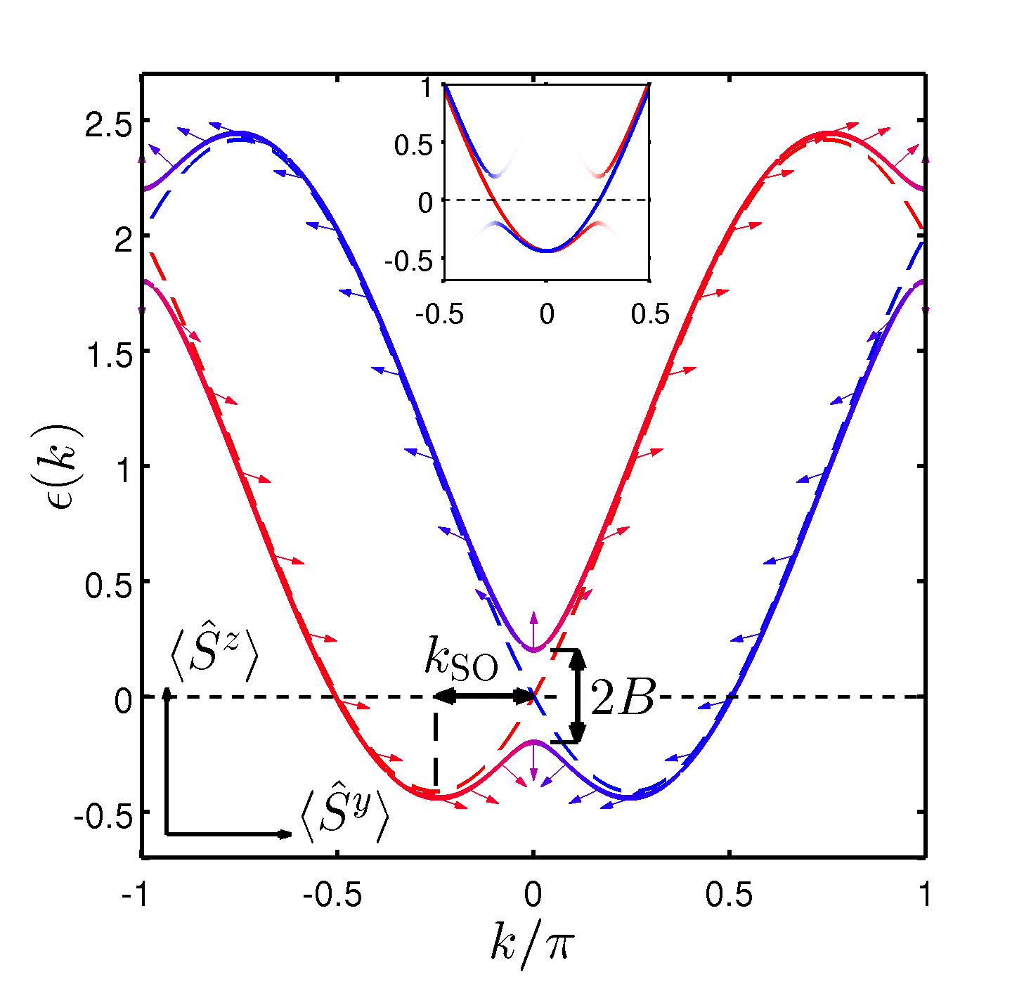
(a) Dispersion

Figure 1: (a) Dispersion $\epsilon(k)$ of the non-interacting Hamiltonian $H_{0}$ with $\alpha=1$, for $B=0.2$ (solid line) and $B=0$ (dashed line). The arrows indicate the spin direction of the eigenvectors (shown only for $B=0.2$), with positive (negative) $\langle\hat{S}^{y}\rangle$ eigenstates displayed in red (blue). The inset shows the dispersion in the gauge transformed basis (eq. (2.3)). Figures (b) and (c) show the dispersions of the corresponding low-energy LLs. The chemical potential is marked by the horizontal dashed lines.

  

(b) Helical LL

(c) Spiral LL

$$k_{\text{SO}}=\arctan\left(\frac{\alpha}{t}\right).$$ (2.2)

Upon turning on the Zeeman field $B$, a gap opens at the crossing points of the two branches at $k=0$ and $k=\pi$, due to the now non-zero coupling between the two branches. The so-called SO gap at $k=0$ is of size $2B$. The ground state has either two Fermi points (2F phase) when the chemical potential is tuned to lie inside the SO gap, or four Fermi points (4F phases) when the chemical potential lies below or above the SO gap (and below the second gap at $k=\pi$). In the so-called helical 2F phase opposite Fermi points have approximately orthogonal spin directions. This is the regime we focus on in this paper. The approximately opposite spin direction at the two Fermi points has some interesting physical implications for e.g. low energy electronic transport, where only excitations close to the Fermi points are relevant. Due to the opposite electron velocities at opposite Fermi points, the charge transport in this regime is highly spin dependent. A right-moving current can only carry negative $\hat{S}^{y}$ electrons, and vice versa for a left-moving current. Another implication is the appearance of a topological, superconducting ground state if an $s$-wave pairing term $c^{\dagger}_{\uparrow}c^{\dagger}_{\downarrow}+h.c.$ is added to the Hamiltonian. In this case, the system becomes a topological $p$-wave superconductor, since only electrons at $+k_{\mathrm{F}}$ and $-k_{\mathrm{F}}$ are available for pairing. It has been shown that the quantum wire in this case hosts Majorana fermions at its edges [49, 10, 11]. To optimally access this phase, the Fermi energy has to be tuned to the center of the SO gap, which is the case if the Fermi momentum $k_{F}=2k_{SO}$. Like for spinless fermions, the relation between the average number of electrons per site $n$ and the Fermi momentum is simply $k_{\text{F}}=n\pi$ inside the SO gap. For $\alpha=1$ (see Eq.(2.2)), we get $k_{\text{SO}}=\pi/4$ and hence the middle of the 2F phase is reached at quarter filling $n=0.5$. One goal of this work is to investigate the effects of electronic correlations on the stability of this 2F phase (see also [48, 50, 51, 52] for related work).

Interactions can be included in several different ways. In this work, we use time-dependent MPS techniques to compute spectral functions, and compare our results to analytic approaches using bosonization techniques. To obtain better comparability to the LL results, we choose a nearest neighbor interaction $U^{\prime}=U/2$ in our numerical calculations (apart from B). This choice minimizes two particle backscattering (scattering from $+k_{\text{F}}$ to $-k_{\text{F}}$), which is a major source of deviation from LL behavior in finite size systems. The two-particle backscattering parameter for the extended Hubbard model is approximately given by $g_{1\perp}=U+2U^{\prime}\cos(2k_{\text{F}})$ [53], which vanishes for $U^{\prime}=\frac{U}{2}$ for $k_{\text{F}}=\pi/2$. In the most part of the present work numerical results are obtained for quarter filling, amounting to $k_{\text{F}}=\pi/2$ in the 2F phase.

In the 2F phase, the low energy physics of our model is captured well by LL theory. In this respect, there exist two related approaches, the helical and the spiral LL [41]. The underlying free dispersions are shown in figure 1a (b) and (c). In the case of the helical LL, the similarity to the dispersion in figure 1a (a) in the 2F phase is evident. Figure 1a (b) and (c) have orthogonal spin directions at opposite Fermi points. The spiral LL figure 1a (c) additionally includes gapped modes. The helical LL may be seen as a low energy model of the spiral LL as long as the relevant excitation energies $\omega$ are smaller than the gap $2B$. The helical LL is very similar to the spinless fermion LL and many properties like density-density correlations are indeed the same.

The relation between the helical and spiral LL approach can be clarified in our model by applying a gauge transformation [40]

$$c_{j}\rightarrow e^{-i\sigma_{y}k_{\text{SO}}j}c_{j}\;.$$ (2.3)

to our model Hamiltonian Eq.(2.1). In the non-interacting case, this yields a modified dispersion relation, as depicted in the inset of figure 1a (a), from which the relation to the spiral LL becomes apparent. By applying this transformation to Eq. (2.1), the SO interaction vanishes, $\tilde{H}_{\mathrm{SO}}=0$, while $H_{\text{t}}$ and $H_{\text{B}}$ in Eq. (2.1) become

$$\begin{split}\tilde{H}_{\mathrm{t}}&=\sum_{j}\left[-\frac{\sqrt{t^{2}+\alpha^{2}}}{2}(c_{j}^{{\dagger}}c_{j+1}+h.c.)-(\mu-t)c_{j}^{{\dagger}}c_{j}\right]\\ \tilde{H}_{\mathrm{B}}&=\sum_{j}B\left[\cos(2k_{\text{SO}}j)c_{j}^{{\dagger}}\sigma^{z}c_{j}-\sin(2k_{\text{SO}}j)c_{j}^{{\dagger}}\sigma^{x}c_{j}\right]\;.\end{split}$$ (2.4)

Note how the site independent magnetic field transforms into a helical field spiraling around the quantum wire, hence the name spiral LL  [41, 38, 39]. The kinetic energy gets rescaled with $t\rightarrow\sqrt{t^{2}+\alpha^{2}}$. Since $H_{\mathrm{int}}$ is unaffected by this transformation, our results are valid for both cases in the commensurate case $k_{\text{F}}=2k_{\text{SO}}$.

2.2 Spectral functions from real-time evolution

In this work we are analyzing the effect of e-e interactions on the spectral properties of a quantum wire, using Matrix Product State (MPS) [54, 55] techniques. MPS are nowadays routinely used in calculations of spectral functions in 1d quantum system. Recent advances include Chebyshev [56, 57, 58, 59, 60, 61] and Lanczos [62, 63] expansion techniques. Here, we obtain real-frequency Greens functions using real time evolution employing the Time Dependent Block Decimation (TEBD) [64, 65] and subsequent Fourier transformation [66, 67, 68, 69]. The object of interest is the Greens function

$$S_{\hat{A}\hat{B}}(k,\omega)=\sum_{j=-\infty}^{\infty}e^{-ikj}\int_{-\infty}^{\infty}dt\,e^{i\omega t}\left(\langle 0|\frac{1}{2}\{\hat{A}_{j}(t),\hat{B}_{0}(0)\}|0\rangle-\langle 0|\hat{A}_{j}(0)|0\rangle\langle 0|\hat{B}_{0}(0)|0\rangle\right),$$ (2.5)

where $\hat{A}_{j}(t)$ and $\hat{B}_{j}(t)$ are operators acting on site $j$ at time $t$, $\{\hat{A},\hat{B}\}=\hat{A}\hat{B}+\hat{B}\hat{A}$ is the anticommutator and $\ket{0}$ is the ground state. For our case of spinors, with $\hat{A}_{j}=c_{j}$ and $\hat{B}_{0}=c^{\dagger}_{0}$, we obtain the spectral function $S_{cc^{\dagger}}(k,\omega)$. The computation proceeds as follows: first, we compute the ground state $\ket{0}$ using DMRG. $S_{cc^{\dagger}}(k,w)$ is then computed from Fourier transformation of the time dependent functions

$$G_{i\sigma,j\sigma^{\prime}}(\omega)\equiv\bra{0}c_{i\sigma}^{\dagger}(t)c_{j\sigma^{\prime}}(0)\ket{0}=e^{iE_{0}t}\bra{0}c_{i\sigma}^{\dagger}e^{-iHt}c_{j\sigma^{\prime}}\ket{0}$$ (2.6)

which are calculated by evolving $\ket{\psi(t)}\equiv e^{-iHt}c_{j\sigma^{\prime}}\ket{0}$ forward in time, and calculating the overlap with $\bra{0}c_{i\sigma}^{\dagger}$. The phase factor $e^{iE_{0}t}$ can be removed by shifting the ground state energy $E_{0}$ of $\ket{0}$ to 0 prior to the evolution.

A common feature shared by all MPS methods for calculating spectral functions is the finite $\omega$-resolution. In our case it is due to the fact that only short to moderately long time scales can be reached with MPS time evolution. This is due to rapid entanglement growth following (local) quenches of the system. The $\omega$-resolution can be substantially improved by using extrapolation techniques for the time series. In this paper we use the so-called linear prediction technique to achieve this [66, 67, 68], see also A. For our study we use system sizes of up to $L=256$ sites, and matrix dimension up to $m=600$ and $m=1200$ for DMRG and during time evolution, respectively, which was large enough to ensure that our results did not depend on the bond dimension $m$ any more. In our code we make use of total charge conservation (note that total $S^{z}$ is not conserved during the time evolution). For the time evolution, we use a second order Suzuki-Trotter splitting scheme, with a time step of $0.05$ ($0.01$ for breather calculations, see below). The dominant error is due to the truncation of the MPS matrices during time evolution. A possible measure of this error is the cumulative truncated weight [66]

$$\epsilon_{\text{tot}}(t)=\sum_{\tau=0}^{t}\sum_{j=1}^{L}\epsilon_{j}(\tau)\;,$$ (2.7)

where the sums run over lattice sites $j$ and time slices $\tau$. Note that the growth of entanglement, and hence $\epsilon_{\text{tot}}(t)$ depend on the particular kind of quench that is applied to the system. For example, for single-particle spectral functions entanglement growth is stronger than for the charge and spin structure factors or the current-current correlation function. Furthermore, for strong interactions the entanglement growth during the time evolution is more pronounced than for weak interactions, while ground states for stronger interactions typically require smaller bond dimensions.

An advantage of our method is the direct accessibility of real frequency spectra without the need of an analytic continuation like in QMC based approaches [70]. It is also considerably more efficient than previous approaches like Dynamical DMRG [71] or the Correction Vector Method [72]. In our approach, spectra at all momenta can be calculated from a single time evolution.

3 Results and Discussion

3.1 Spectral functions

We now move on to analyze the effect of e-e interaction on spectral functions of the quantum wire. Results are shown in figure 2a. The data was obtained from evolving Eq. (2.6) up to $t_{\text{max}}=25$ on a system with $L=128$ sites. Using linear prediction, the time series was extrapolated to $t_{\mathrm{LP}}=275$. We note that at larger interaction strengths the truncation error $\epsilon_{\text{tot}}(t)$ grows more rapidly with $t$  . We have checked all our results for convergence in $m$. The spectrum in figure 2a (a) at $U=0.5$ exemplifies the spectral resolution of our approach.

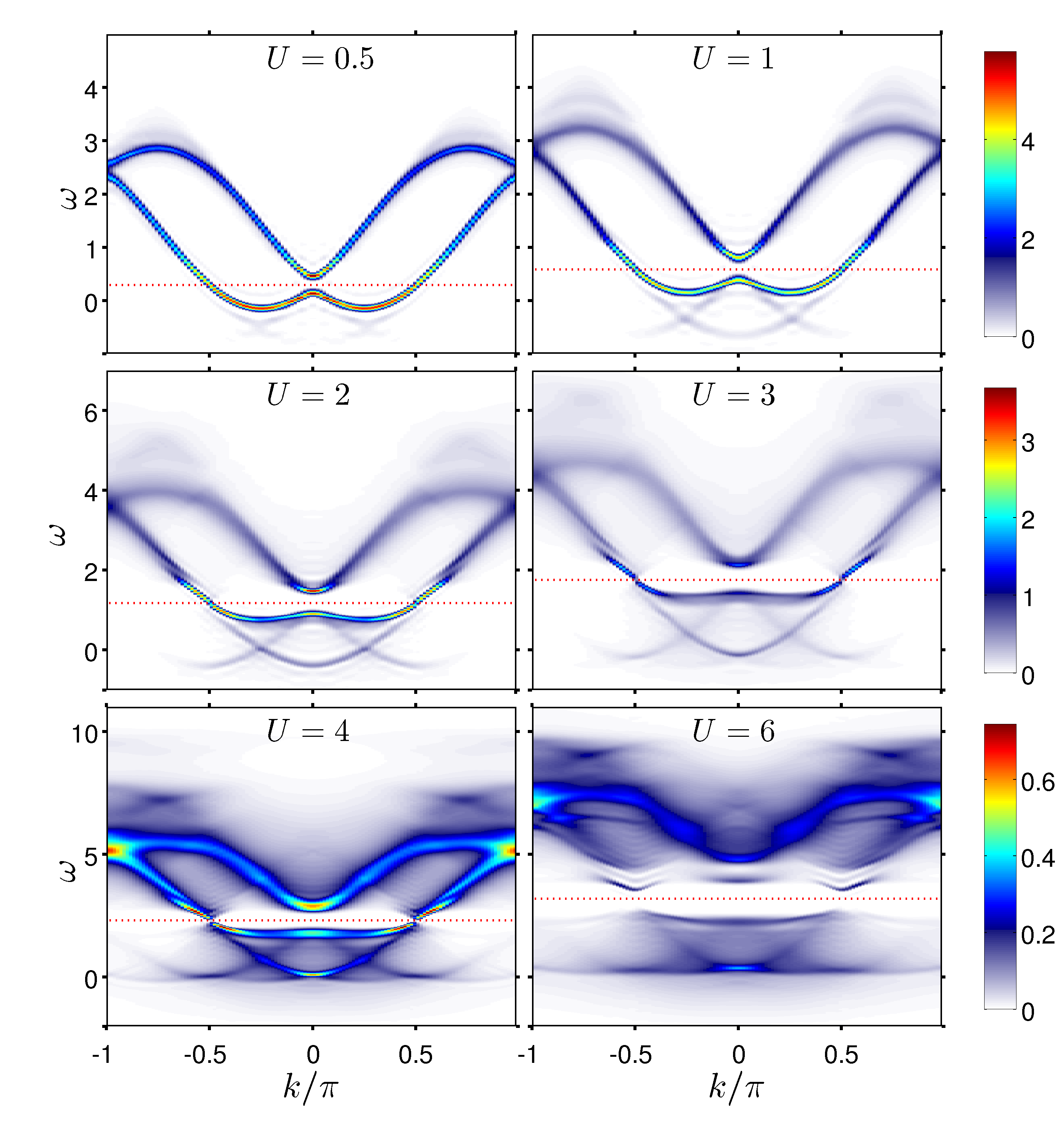
(a)

Figure 2: (a) Spectral function $S_{cc^{\dagger}}(k,\omega)$ for $n=0.5$, $\alpha=1$, $B=0.1$ and several values of $U$ (with $U^{\prime}=U/2$, system size $L=128$ and $N=nL$ fermions). The dotted red line is the Fermi energy, determined from the ground state energies as $E_{F}=(E(L,N+1)-E(L,N-1))/2$. (b) SO gap parameter $B^{*}$ as obtained from the gap of size $2B^{*}$ in the spectral functions (shown until the MI phase sets in at $U=4$). Results for $U^{\prime}=0$ are reported in B.

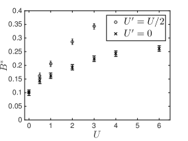
(b)

Figure 2a (a) shows the evolution of the spectral function with the Coulomb interaction $U$, for $\alpha=1$, $B=0.1$, and at $U^{\prime}=U/2$ for which the two-particle backscattering is suppressed at quarter filling. For comparison spectral function for $U^{\prime}=0$ are shown in B. With increasing interaction, the two noninteracting branches get significantly broadened, but remain visible up to large values of $U=6$. Close to the Fermi energy, the spectral functions remain sharp, as predicted by the LL theory. The bandwidth increases with the interaction, and so does the SO gap. This is shown in figure 2a (b). Within the spiral LL approximation, the correlation-induced enhancement of the gap in the is found to be [38, 39, 73, 74]

$$2B^{*}=2B\xi^{1-\kappa/2}\;,$$ (3.1)

where $\kappa=K_{\rho}+K_{\sigma}^{-1}$ is determined from charge and spin LL parameters $K_{\rho}$ and $K_{\sigma}$ and a correlation length $\xi$. For the noninteracting system, $K_{\rho}=K_{\sigma}=1$ and $B^{*}=B$. Repulsive interactions, for which $K_{\rho}<1$ and $K_{\sigma}>1$, lead to $\kappa<2$. As a consequence, the SO gap is enhanced by the interactions, which is confirmed by figure 2a (b).

For $U=6$, the opening of a gap at $\pm k_{\mathrm{F}}$ indicates the emergence of a Mott insulating (MI) phase at quarter filling [1, 75, 76, 77], as described in section 3.2. We note that the MI phase is absent for $U^{\prime}=0$, see B.

If the momentum shift of the SO interaction is removed by the gauge transformation Eq. (2.3) , the similarity to the dispersion of the Hubbard model facilitates the interpretation of the other features of the spectral functions. Figure 3 (a) shows that below the Fermi level several dispersing branches appear, originating from the spin-charge separation. The distinctive main branch and the two weaker ones below can be attributed to the collective spinon and holon excitations [78, 79], respectively. The spectral weight of both increases with increasing interaction.

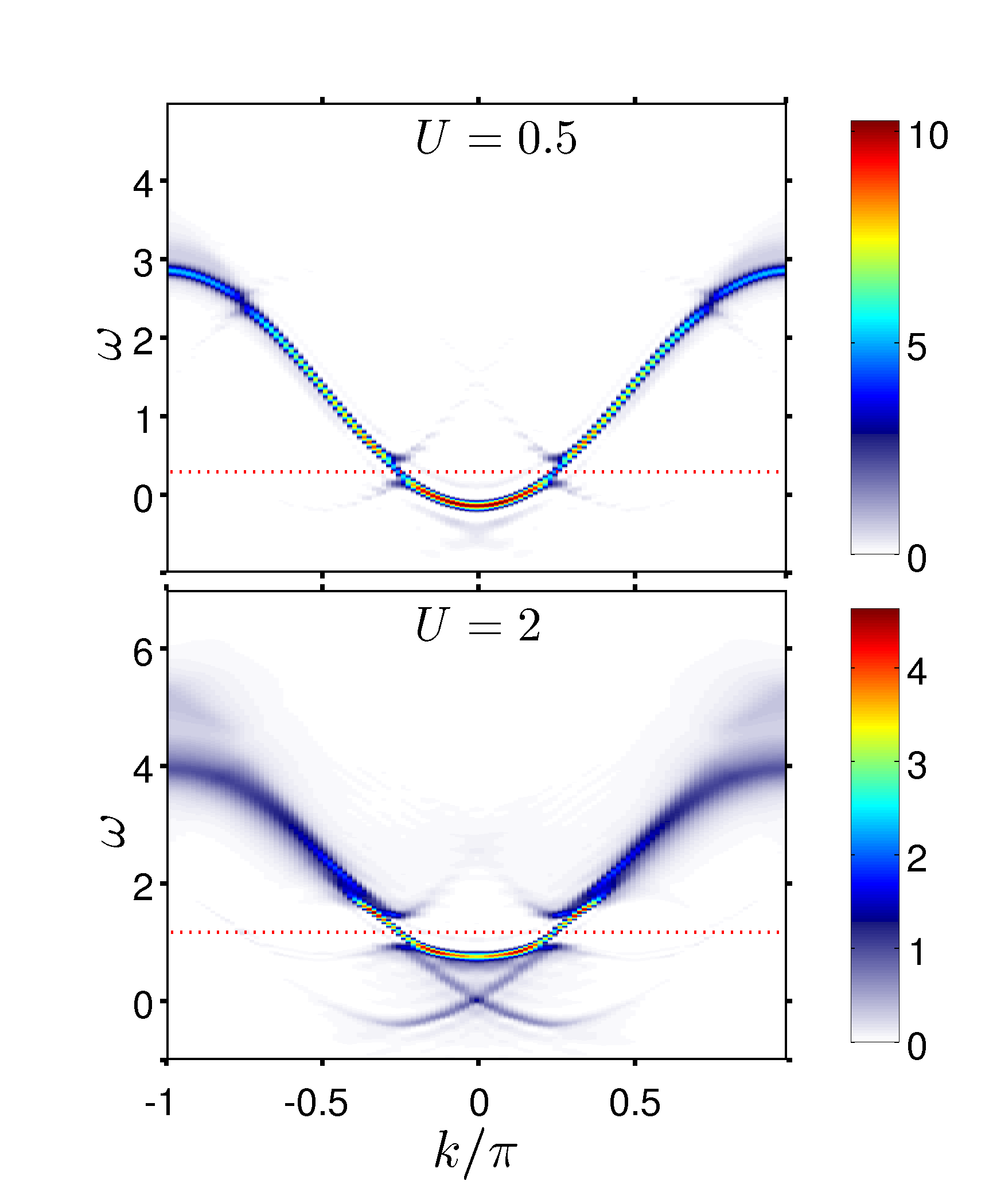
(a)

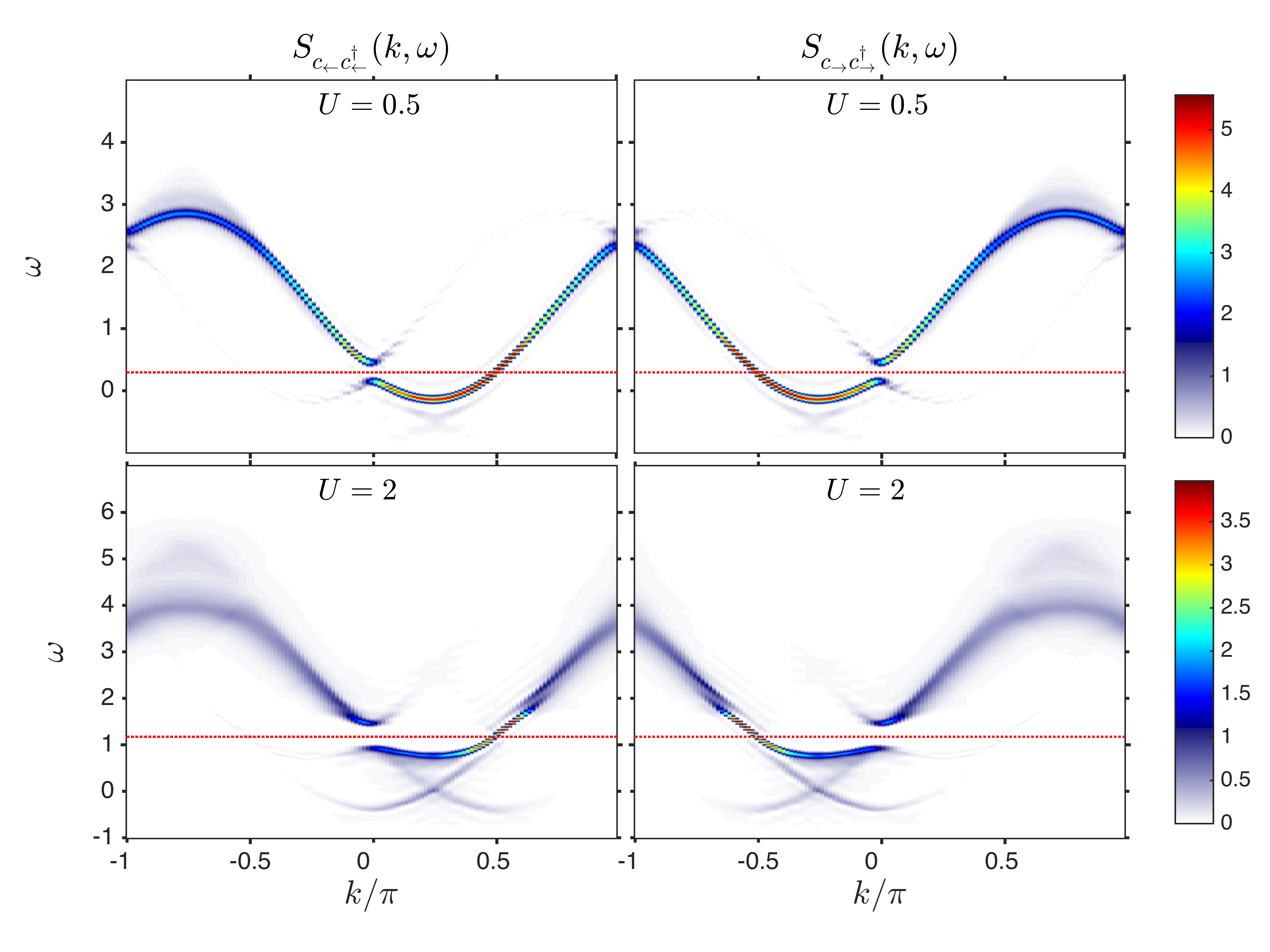
(b)

Figure 3: (a) Spectral function in the gauge-transformed basis, at $n=0.5$, $\alpha=1$, $B=0.1$, $L=128$ and different values of $U$. (b) Spectral functions for individual spin components, parallel or antiparallel to the SO interactions, for the same couplings as in (a). The spectra in (a) were obtained from the sum of the spectral functions of (b) shifted by $\pm k_{\text{SO}}$.

In figure 3 (b) we show the spin-resolved components of the spectral functions for the parallel and antiparallel direction with respect to the SO interaction (see arrows in figure 1a), as determined by Eq.(2.5) for $c^{\dagger}_{\rightarrow}=(c^{\dagger}_{\uparrow}+ic^{\dagger}_{\downarrow})/\sqrt{2}$ and $c^{\dagger}_{\leftarrow}=(c^{\dagger}_{\uparrow}-ic^{\dagger}_{\downarrow})/\sqrt{2}$. These directions are of particular interest, since they determine the spin-dependent transport properties. Each spin direction contains only a single Fermi point with non-negligible spectral weight. Thus we find that the helical spin order is robust with respect to electronic correlations and that spin transport is still polarized. Since $n=0.5$, the SO gap opens at $k_{\text{F}}$ like for the spiral LL dispersion displayed in figure 1a (c).

Summarizing, the correlation effects observed for the microscopic model are in agreement with the LL predictions of an enhanced SO gap in the spectral functions and of the preservation of the helical spin order with spin-dependent transport within the metallic 2F phase [38, 39, 42, 48].

3.2 Phase diagrams

3.2.1 Spiral and helical phases.

In many applications – like Majorana wires, spin filters and Cooper pair splitters – it is crucial that the system is in the helical 2F phase [10, 11, 20, 21, 23]. Therefore, and in order to guide experimental realizations, we investigate the phase boundaries between the ordinary 4F phases and the helical 2F phase. In principle, the number of Fermi points can be obtained by simply counting them in the spectrum. However, the calculation of spectral densities at many sets of parameters is computationally rather expensive as compared to e.g. ground state calculations. Therefore, a reliable method to find the number of Fermi points based only on ground state properties is favorable.

(a)

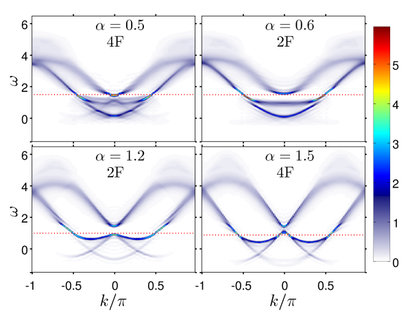
(b)

Figure 4: (a) Phase diagram ($\alpha$,$U$), for $n=0.5$, $B=0.1$ and $L=128$. The phase boundaries between the 2F and 4F phases are obtained from the discontinuity in $K_{\rho}$ (Eq. (3.3)). The phase boundary of the MI was obtained from the closing of the two particle charge gap in DMRG. The red and green lines are polynomial fits (using second order for the lower red line and first order for the upper red and green lines). (b) Spectra in the 4F and 2F phases at $U=2$ for different SO interactions $\alpha$.

To this end, we use a method based on the calculation of the static density-density correlation function $C_{\hat{n}\hat{n}}(r)\equiv\bra{0}\hat{n}_{r}\hat{n}_{0}\ket{0}$. Within the 2F phase, our system is described by a spinless fermion LL, and the asymptotic behavior ($1\ll r\ll L$) of the density-density correlations is given by [80]

$$C_{\hat{n}\hat{n}}(r)\sim-\frac{K_{\rho}}{2(\pi r)^{2}}+A\frac{\cos(2k_{\text{F}}r)}{r^{1+K_{\rho}}}\ln^{-\frac{3}{2}}(r)+...,$$ (3.2)

with a model-dependent constant $A$. The second expression contributes only logarithmically and is neglected. After a Fourier transformation, $K_{\rho}$ can be obtained from the derivative at $k=0$ in the thermodynamic limit, or from a finite size extrapolation of $L\rightarrow\infty$:

$$K_{\rho}=\lim_{L\rightarrow\infty}L\,\tilde{C}_{\hat{n}\hat{n}}(k=\frac{2\pi}{L}).$$ (3.3)

In the 4F phase on the other hand, the low energy physics is no longer described by the simple LL for spinless fermions. Nevertheless, the leading large-distance behavior of the density-density correlations is still quadratic, namely $K_{\rho}/(\pi r)^{2}$. Thus the change in the prefactor of $1/r^{2}$, by a factor of $2$, can be used to distinguish the 2F and 4F phases.

The phase diagrams obtained in this way are shown in figures 4 (a) and 5 (a). For the phase boundaries between 2F and 4F phases (red lines in figures 4 (a) and 5 (a)) we used a system size of $L=128$ (the results for $L=256$ are indistinguishable from $L=128$). In figure 4 (a), the phase boundary to the MI (green line) was obtained from the closing of the two particle charge gap (see below). The inset in figure 5 (a) shows the behavior of the LL parameter $K_{\rho}$ as determined by Eq. (3.3), with the jump at the phase boundaries between the 2F and 4F phases. Except for $U=0$, the actual jump of $K_{\rho}$ between the two phases is in general smaller than a factor of 2 .

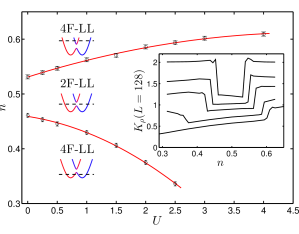
(a)

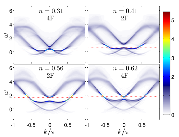
(b)

Figure 5: (a) Phase diagram ($n$,$U$), for $\alpha=1$, $B=0.1$ and $L=128$. The phase boundaries between the 2F and 4F phases are obtained from the discontinuity in $K_{\rho}$ (see Eq. (3.3)). The inset shows the behavior of $K_{\rho}$ for different values of $U=0$, $0.5$, $1$, $2$, $3$ from top to bottom. The red lines are polynomial fits of second order. (b) Spectra in the 4F and 2F phases at $U=2$, for different fillings $n$.

The phase boundaries in $(\alpha,U)$ (figure 4) were obtained at quarter filling $n=0.5$, and in $(n,U)$ at $\alpha=1$ (figure 5). In the noninteracting case, the boundaries of the 2F phase in $(\alpha,U=0)$ (at $n=0.5$) are at

$$\sqrt{t^{2}-2Bt}<\alpha<\sqrt{t^{2}+2Bt}\;,$$ (3.4)

and in $(n,U=0)$ for fixed $\alpha$ at

$$\arccos\left(\frac{t^{2}-\alpha^{2}+2Bt}{t^{2}+\alpha^{2}}\right)<\pi n<\arccos\left(\frac{t^{2}-\alpha^{2}-2Bt}{t^{2}+\alpha^{2}}\right)\;.$$ (3.5)

The phase boundaries at $U=0$ obtained from Eqs. (3.4) and (3.5) lie within the error bars of the numerically obtained ones in figure 4 and 5.

Remarkably, we find that with interactions the parameter range of the 2F phase gets greatly enhanced [48], which is in accordance with the interaction-enhanced gap we already found for the spectral functions in figure 2a (a). Examples for spectral functions in the different phases are given in figures 4 (b) and 5 (b). We show the spectral functions in the proximity of the phase boundaries. Note how the SO gap gets enhanced as soon as the Fermi energy slips inside the 2F phase. Therefore, we predict repulsive electron-electron interactions to be beneficial to applications depending on the 2F phase, like Majorana zero modes [48, 58, 81, 82] or spin-filters.

For both phase diagrams (figures 4 and 5), the jump in $K_{\rho}$ (only shown in figure 5) is no longer visible in the strong coupling regime, indicating that the LL picture breaks down there.

3.2.2 Mott phase.

At quarter filling, the strong coupling phase is a Mott Insulator [1, 75]. To detect the MI phase transition in our model, we use two different approaches, to be detailed in the following. The first one is via the calculation of the two-particle (charge) excitation gap above the ground state,

$$\Delta_{L}^{2}=\frac{1}{2}\bigl{[}E(L,N+2)+E(L,N-2)-2E(L,N)\bigr{]}\;,$$ (3.6)

with $N$ being the absolute filling $N=nL$. In the absence of pairing effects, the two particle and the single particle excitation gap will scale to the same value in the thermodynamic limit, but the two particle excitation gap is robust to even/odd effects. $\Delta_{L}^{2}$ is calculated from ground state energy of three different $DMRG$ runs, one for each total filling $N+2,N$ and $N-2$. Complementary to this, we use the evolution of $K_{\rho}$ with increasing $U$ to detect the MI phase transition. For quarter filling, there is a critical value $K_{\rho}^{*}=0.25$ below which the system is in a MI state [1]. Note that the value of $K_{\rho}$ from Eq. (3.3) in the 4F phase, Eq. (3.3), differs by a factor of two as compared to the 2F case, see the discussion in Sec. 3.2.1. For both approaches, the values in the thermodynamic limit $L\rightarrow\infty$ were obtained by a polynomial fit in $1/L$, as shown in the right column of figure 6 (a). The left column in figure 6 (a) shows the results in the thermodynamic limit $L=\infty$. The phase boundaries obtained from the two approaches agree within the error bars and are shown as the green line in figure 4 (a). Note how the phase boundary to the MI moves to larger values of $U$ with increasing SO interaction. This can be understood from the contribution of the SO interaction to the kinetic energy of the system, which lowers the effective interaction at fixed $U$ and drives the system away from the MI.

The charge gap in the MI is also clearly visible in the local density of states LDOS${}_{j=1}(\omega)$ at the left chain boundary, as shown in figure 6 (b). In the LL phase we find a pronounced interaction-induced suppression of the local spectral weight [83, 84], while in the Mott phase a gap opens around the Fermi energy. The high-energy peak in the LDOS corresponds to the upper Hubbard band, see also figure 2a.

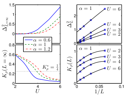
(a)

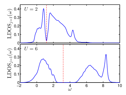
(b)

Figure 6: (a) The boundary to the MI as a function of $U$ was determined from the charge gap (upper left panel) $\Delta^{2}_{L=\infty}$ as well as from the critical value of $K_{\rho}^{*}=0.25$ (lower left panel). The finite-size extrapolations are shown for $\alpha=1$ in the right panel (using system sizes $L=\{16,32,64,128$}). (b) Local density of states at the chain boundary for $U=2$ (in the LL phase) and $U=6$ (in the MI phase), both at $\alpha=1$. The dotted red line is the Fermi energy. For all panels the other parameters are $n=0.5$, $B=0.1$ and $L=128$.

Away from quarter filling, a strong coupling region emerges at strong interactions which is further examined in C.

3.3 Breathers, structure factors and optical conductivity

3.3.1 Breather bound states.

In the mathematical formulation of the spiral LL, the gapped modes are described by a sine-Gordon model (SGM). The elementary excitations in the SGM are solitons and antisolitons with the mass $B^{*}$ of half the SO gap. In the attractive regime of the SGM (which amounts to repulsive interactions in the spiral LL), additional soliton-antisoliton bound states appear, which are so-called breather states [85, 86]. In the spiral LL theory their masses are given by [42]

$$\Delta_{l}=2B^{*}\sin\left(\frac{l\pi\kappa}{8-2\kappa}\right)\;,$$ (3.7)

with $l=1,\dots,l_{\text{max}}$ and $l_{\text{max}}=\text{int}(4/\kappa-1)$ different breathers (for $\kappa<2$, with $\kappa=K_{\rho}+1/K_{\sigma}$).

Figure 7: Illustration of breather bound states on the gapped modes, consisting of a particle excitation (soliton) on the upper branch and a hole excitation (antisoliton) on the lower branch. The spectral function shown here was obtained for $n=0.5$, $\alpha=1$, $U=1$, $B=0.3$ and $L=128$.

In our lattice model the breathers correspond to bound states of a particle excitation (soliton) and a hole excitation (antisoliton) on the gapped modes (see figure 7 for an illustration). They are charge neutral but carry a positive $\hat{S}^{z}$ magnetization. The electron and the hole are bound together by the interaction, with an energy smaller than the SO gap $2B^{*}$. In the real-time evolution, breathers oscillate back and forth around their “center of mass”, which motivates their naming. The breather contributions to one-particle Green functions, like the spectral function or the local density of states, are found to be negligible [42]. However, the breathers strongly couple to the current density $\hat{J}$, hence the optical conductivity

$$\sigma(\omega>0)=\frac{\text{Im}(S_{\hat{J}\hat{J}}(k=0,w>0))}{L\omega}$$ (3.8)

is an excellent choice for observing breather bound states.

In the following, we will compare the optical conductivity $\sigma(\omega)$ of our microscopic model to the optical conductivity $\sigma_{SLL}(\omega)$ of the spiral LL, which has been calculated in Ref. [42]. We will determine the necessary parameters $B^{*}$, $K_{\rho}$, $K_{\sigma}$ and the charge and spin velocities $v_{\rho}$ and $v_{\sigma}$ for the calculation of $\sigma_{SLL}(\omega)$ from our microscopic model. This comparison will serve as an important test for the consistency and validity of the spiral LL approach and our numerical calculations.

Since we are now focusing on the physical behavior taking place at energies smaller than the SO gap, it is advantageous to use a stronger Zeeman field of $B=0.3$ for a wider gap. The other parameters are as before, $\alpha=1$ and $n=0.5$, different interactions $U$, and $U^{\prime}=U/2$. The higher magnetic field $B=0.3$ causes the MI phase to set in earlier (from $U\geq 2$ on there are hints of a quarter filled MI order). We extracted the values of the spiral LL parameters from several different observables.

3.3.2 Local density of states.

The renormalized size $2B^{*}$ of the SO gap was extracted from the local density of states (LDOS) in figure 8. Due to the local nature of the LDOS we were able to use longer time evolutions than for the momentum-resolved spectra in the same systems, reaching from $t_{\text{max}}=30$ up to $t_{\text{max}}=90$ depending on the interaction. The small scale oscillations visible in figure 8 at lower values of the interaction are consistent with the energy spacing for an $L=128$ site system. Results for $B^{*}$ are shown in table 1.

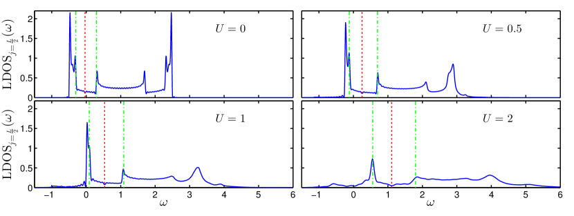
Figure 8: Local density of states in the middle of a $L=128$ site chain for $n=0.5$, $\alpha=1$, $B=0.3$ and different values of $U$. The dashed red line is the Fermi energy, whereas the dot-dashed green lines mark the boundaries of the SO gap.

$U$	$K_{\rho}$	$K_{\sigma}$	$v_{\rho}$	$v_{\sigma}$	$B^{*}$	$\Delta_{1}$
0	1.00	1.00	1.0	1.0	0.30	—
0.5	0.87	1.20	1.0	1.0	0.41	0.75 (0.75)
1	0.76	1.28	1.0	1.1	0.50	0.83 (0.83)
2	0.59	1.29	1.2	1.3	0.62	0.89 (0.90)

Table 1: Parameters $K_{\rho}$, $K_{\sigma}$, $v_{\rho}$, $v_{\sigma}$ and $B^{*}$ as used for the field-theoretical calculations, and the mass of the first breather $\Delta_{1}$. $K_{\sigma}$ was extracted from the energy of the first breather peak $\Delta_{1}$ using Eq. (3.7), where $\Delta_{1}$ was obtained from the position of the peak in figure 10. The value in parentheses is obtained from the oscillation frequency in figure 11. The estimated uncertainties in these values are about 5% (10% for the velocities).

3.3.3 Structure factors.

We obtain the velocities $v_{\rho}$ and $v_{\sigma}$ from the corresponding structure factors $S_{\hat{n}\hat{n}}(k,\omega)$ and $S_{\hat{S}^{y}\hat{S}^{y}}(k,\omega)$. The structure factors are shown in figure 9. Since the spectra are symmetric, values for $k<0$ are not shown. Near $k=\omega=0$, the dispersions are approximately linear (at least for the considered $U\leq 2$) and the velocities were obtained from fits to their slopes. Table 1 shows that for the interactions considered, $v_{\rho}\approx v_{\sigma}$.

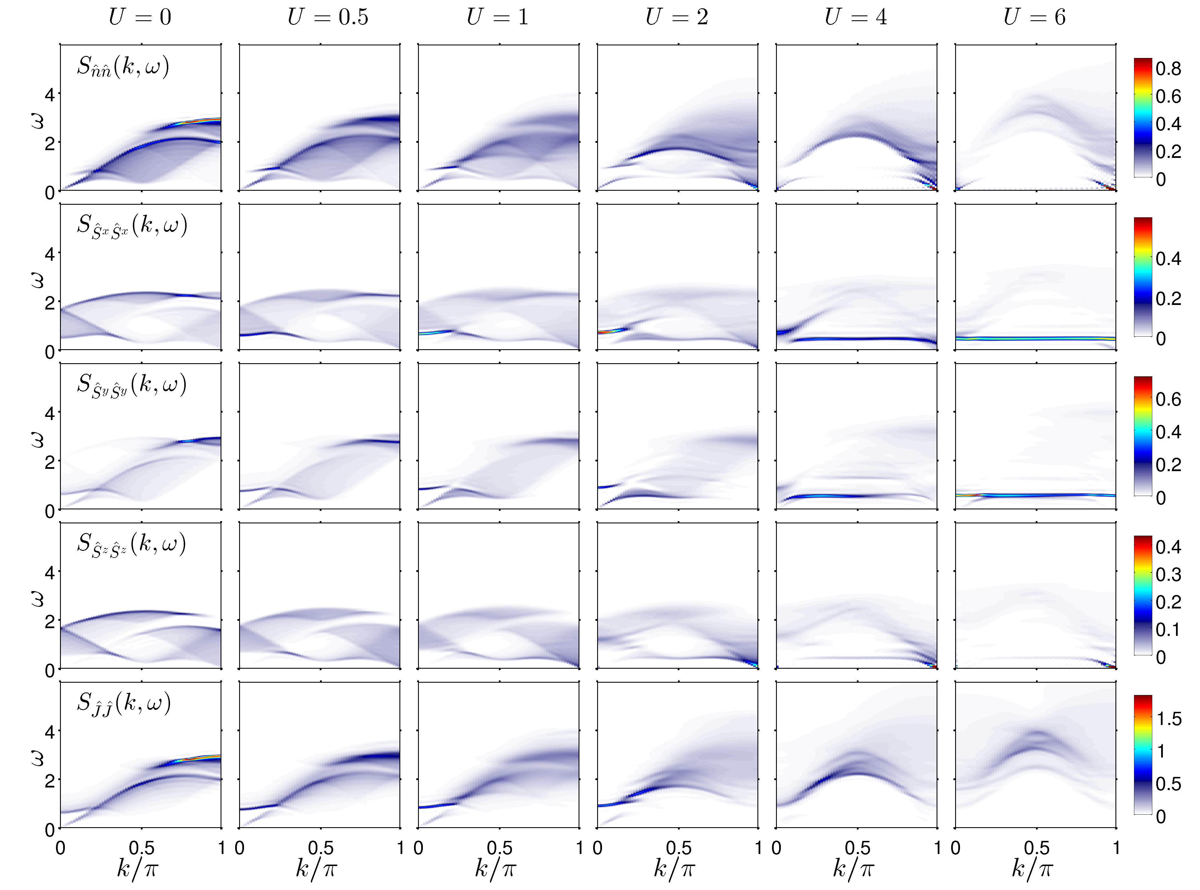
Figure 9: Charge, spin and current structure factors $S_{\hat{n}\hat{n}}(k,\omega)$, $S_{\hat{S}^{x}\hat{S}^{x}}(k,\omega)$, $S_{\hat{S}^{y}\hat{S}^{y}}(k,\omega)$, $S_{\hat{S}^{z}\hat{S}^{z}}(k,\omega)$ and $S_{\hat{J}\hat{J}}(k,\omega)$, for $n=0.5$, $\alpha=1$, $B=0.3$, $L=128$ and different values of $U$. $S_{\hat{n}\hat{n}}(k=\pi,\omega=0)$ and $S_{\hat{S}^{z}\hat{S}^{z}}(k=\pi,\omega=0)$ diverge in the MI phase ($U>2$) and exceed the color range, with maximal values in our analysis of $1.0$, $20.4$, $42.4$ for $S_{\hat{n}\hat{n}}(k,\omega)$ and of $0.5$, $4.8$, $7.9$ for $S_{\hat{S}^{z}\hat{S}^{z}}(k,\omega)$ at $U=2$, $4$, $6$ respectively.

The structure factors themselves contain very interesting physics. In the weak coupling regime, the nearly linear dispersions starting at $k=\omega=0$ visible in $S_{\hat{n}\hat{n}}(k,\omega)$, $S_{\hat{S}^{y}\hat{S}^{y}}(k,\omega)$ and $S_{\hat{J}\hat{J}}(k,\omega)$ result from the ungapped modes of the Hamiltonian. The approximately quadratic dispersion at $\omega=\Delta_{1}$ and $k=0$ in $S_{\hat{S}^{x}\hat{S}^{x}}(k,\omega)$, $S_{\hat{S}^{y}\hat{S}^{y}}(k,\omega)$ and $S_{\hat{J}\hat{J}}(k,\omega)$ corresponds to the breather modes. Note that their dispersion starts at an energy $\Delta_{1}$, which is smaller than the SO $2B^{*}$ gap obtained from the single-particle spectra. The breather dispersion gains more spectral weight with increasing interaction but smears out in the MI phase from $U\geq 2$ on. Unlike spin charge separation, which also gives rise to two low energy modes [87], the modes here are not separated because of interactions but due to the interplay of Zeeman field and SO interaction (each mode is a combination of spin and charge degrees of freedom).

In contrast to an ordinary MI, at quarter filling there is no antiferromagnetic order at $k=\pi/2$ in the spin structure factors. Instead, the Zeeman field induces a finite magnetization. Therefore, $S_{\hat{S}^{z}\hat{S}^{z}}(k,\omega)$ and $S_{\hat{n}\hat{n}}(k,\omega)$ show the same diverging behavior at $k=\pi$ and $\omega=0$ for strong interactions. Deep in the MI phase, $S_{\hat{S}^{x}\hat{S}^{x}}(k,\omega)$ and $S_{\hat{S}^{y}\hat{S}^{y}}(k,\omega)$ consist almost solely of a constant energy level at $\omega=2B$, indicating that all movement of the spins freezes except for a simple precession around the Zeeman field. $S_{\hat{n}\hat{n}}(k,\omega)$ and $S_{\hat{S}^{z}\hat{S}^{z}}(k,\omega)$ are dominated by the Mott instability for strong interactions. As soon as the interactions are turned on, spectral weight at $\omega=0$ and $k=2k_{\mathrm{F}}=\pi$ accumulates, indicating the charge order of the quarter filled MI. In the MI phase, $S_{\hat{n}\hat{n}}(k,\omega)$ and also $S_{\hat{S}^{z}\hat{S}^{z}}(k,\omega)$ diverge at this point.

The LL parameter $K_{\rho}$ at $B=0.3$ was obtained from the static density-density correlations, as described in section 3.2. We used system sizes from $L=16$ up to $L=256$ and extrapolated to $L=\infty$ by a fourth order polynomial fit in $1/L$. The spin parameter, $K_{\sigma}$, is known to be very susceptible to finite size corrections [88]. When we applied the same method to $K_{\sigma}$, we found the extrapolation to the thermodynamic limit to be unreliable, since it turned out to be nonmonotonic in $1/L$. Since all other parameters for the field theory are already fixed, we choose to obtain $K_{\sigma}$ with Eq. (3.7) from the energy of the breather peak in the optical conductivity $\sigma(\omega)$, which we discuss now.

3.3.4 Optical conductivity.

According to Eq. (3.8) the optical conductivity can be obtained from $S_{\hat{J}\hat{J}}$. For our model, the usual Hubbard current operator has to be adapted in order to include the SO interaction. It then reads as follows for the current between the sites $j$ and $j+1$

$$\hat{J}_{j}=i\left[-\frac{t}{2}\sum_{\sigma}(c_{j\sigma}^{\dagger}c_{j+1\sigma}-c_{j+1\sigma}^{\dagger}c_{j\sigma})+\frac{\alpha}{2}(c_{j\downarrow}^{\dagger}c_{j+1\uparrow}-c_{j+1\uparrow}^{\dagger}c_{j\downarrow}-c_{j\uparrow}^{\dagger}c_{j+1\downarrow}+c_{j+1\downarrow}^{\dagger}c_{j\uparrow})\right]\;.$$ (3.9)

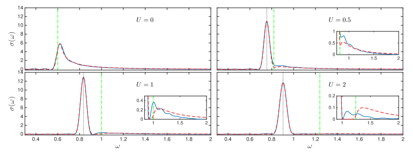
Figure 10: Optical conductivity $\sigma$ for $n=0.5$, $\alpha=1$, $B=0.3$, $L=200$, and different values of $U$. The numerical result (solid blue line) is compared to the field-theoretical result (dashed red line) [42]. The dot-dashed green line marks the SO gap $2B^{*}$ as obtained from figure 8. The dotted black line shows the extracted breather energy. The insets zoom into the soliton-antisoliton continuum for better visibility.

.

The further calculation of $\sigma(\omega)$ is analogous to the spectral densities and structure factors. We calculated the time evolutions on a $L=200$ site system until $t_{\mathrm{max}}=42.5$. A matrix dimension of $m=1200$ was used. We observed that the entanglement grows slower with a $\hat{J}$ excitation than a single particle excitation. Therefore, longer simulation times were feasible at a comparable $\epsilon_{\text{tot}}$. Linear prediction was used up to time 140.5. The time series was then multiplied with a window function of Dolph-Chebyshev type. The optical conductivity $\sigma(\omega)$ of our microscopic model is presented in figure 10  .

We are now ready to compare $\sigma(\omega)$ to the field theoretical result $\sigma_{SLL}$ in a spiral LL [42]. The parameters for the field theoretical calculations are shown in table 1. Apart from $K_{\sigma}$, which was extracted from the energy of the breather peak depicted by the dotted black lines in figure 10, all other parameters were obtained from calculations independent of the optical conductivity.

The field theoretical result, $\sigma_{SLL}(\omega)$, was convoluted with a Dolph-Chebyshev window, the same way as the numerical data, and scaled such that the breather peak heights coincide, see figure 10. Its shape agrees very well with the numerical result both in the interacting and in the noninteracting case. In the latter there is no breather satisfying Eq. (3.7), instead the peak is given by the onset of the soliton-antisoliton continuum at $\omega=2B$. This onset is moved to $\omega=2B^{*}$ in the interacting case. The insets show the soliton-antisoliton continuum in detail. We believe that the small-scale oscillations are artifacts originating from the window function. At nonzero interactions, the breather contribution at energies $\omega=\Delta_{1}<2B^{*}$ emerges, which in the field theory takes the form $\sim\delta(\omega-\Delta_{1})$. We note that we are always in the parameter range $4/3\leq\kappa<2$, where only a single breather exists. Generally, we observe that the intensity of the field theoretical result drops more slowly at high energies than in our numerical calculations, which may originate from the existence of a finite band width in our lattice model. To sum up, we conclude that our simulations for the optical conductivity are in good agreement with the field theoretical results.

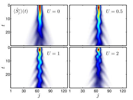
Figure 11: Time evolution of $\langle\hat{S}^{z}\rangle$ after an excitation (3.10) for $n=0.5$, $\alpha=1$, $B=0.3,L=128,$ and different values of $U$.

3.3.5 Time evolution of breather bound states.

It is interesting, and potentially relevant for experiments, to visualize the breather oscillations directly, by examining the time evolution of the system after a local excitation from the ground state. A gaussian density excitation, centered around $k=0$, is suitable for this task:

$$|\psi(t=0\rangle=g^{\dagger}_{k=0}g_{k=0}|0\rangle,~{}~{}~{}\text{where}$$ (3.10)

$$g_{k}=\sum_{j}e^{-\frac{(j-j_{0})^{2}}{2\tilde{\sigma}^{2}}}e^{i(j-j_{0})k}(c_{j\uparrow}^{\dagger}+c_{j\downarrow}^{\dagger})\;.$$

We take $\tilde{\sigma}=4$, which corresponds to a width of $0.25$ in $k$-space. By employing an excitation in the eigenstate direction $(c_{j\uparrow}^{\dagger}+c_{j\downarrow}^{\dagger})$ with positive $\hat{S}^{x}$-eigenvalue, we ensure that the excitation can act on both branches of the dispersion simultaneously. The breather state itself has a positive magnetization $\hat{S}^{z}$, which we use as the observable in figure 11. The zigzag oscillations of the breather state are clearly visible in the time evolution, with the frequency of the oscillation corresponding to its energy. The oscillations at $U=0$ reflect the onset of the soliton-antisoliton continuum at $\omega=2B$. The breather energies in the optical conductivity and for the direct excitation are in good agreement, see table 1. We observe that at $U=0.5$ and $U=1$ the oscillations are longer lived than at $U=2$, which is a sign of the onset of the Mott instability in the latter case.

4 Conclusions and Outlook

We have presented a detailed analysis of the static and dynamic properties of strongly correlated quantum wires with Rashba SO interaction and Zeeman field. We investigated a microscopic model, with SO interaction, Zeeman field and tunable interactions of extended Hubbard type, and calculated the static and dynamic properties by DMRG and TEBD. We assessed the validity of the field-theoretical description by comparing the results for the microscopic model to the predictions for the corresponding low energy models, the helical and spiral LL. In particular, we confirmed the enhancement of the SO gap with increasing Coulomb interaction. Furthermore, from the LL parameters we determined the phase diagram of the system. We found that the parameter range (in filling, respectively SO interaction) of the metallic 2F phase increases in the presence of interactions, and that helical spin order and spin-dependent transport are preserved. This means that interactions are a way to increase the SO gap without disturbing the helical spin order (which a larger magnetic field would do). The interesting 2F phase thus becomes more accessible in presence of interactions, which is very welcome in view of future applications exploiting the helical spin order like spin-filters, Cooper-pair splitters and Majorana wires [10, 11, 20, 21, 23]. The main prediction of our work with respect to Majorana experiments is the interaction enhancement of the SO gap. In principle, this could be detected by measuring the Landé $g$-factor in the nanowires. To make a direct comparison, more information on the interaction strength in semiconductor nanowires would be required, though. For very strong interaction strengths, however, the 2F phase is suppressed in favor of a Mott insulating phase in the commensurate case, characterized by the opening of a charge gap.

Furthermore, we analysed characteristic breather bound states in the optical conductivity $\sigma(\omega)$ as predicted for the spiral LL. Using the extracted LL parameters, the optical conductivity was found to be in good agreement with the field-theoretical results. Finally, we showed the presence of strong oscillatory behavior in the time evolution of the bound states after an excitation, which can provide a route for their experimental detection i.e. in cold atom systems.

While the present work focuses on the 2F phase, the LL theory predicts interesting phases hosting fractional excitations if the chemical potential is tuned below the SO gap [90, 43, 91, 92, 93]. Using our methods, a systematic study of these fractional phases in a microscopic model could be addressed.

Appendix A Linear prediction

The linear-prediction technique approximates future values of an equally spaced time series $\{y_{i}\}$ as a linear combination of past values [66, 94, 68]

$$x_{l}\approx\tilde{x}_{l}=-\sum_{j=1}^{N}a_{j}x_{l-j}\;.$$ (1.1)

The coefficients $a_{j}$ are determined by minimizing a least squares error. Linear prediction efficiently extrapolates future data points as a sum of damped exponentials, respectively Lorentzians after the Fourier transformation, which is justified in many cases. Due to the large number of coefficients $a_{j}$, other functions can be represented with sufficient accuracy as well. We use $N_{\text{max}}/2$ coefficients, with $N_{\text{max}}$ being the number of steps in our time evolution. The numerical effort of the prediction is negligible compared to the time evolution itself.

Appendix B Spectra for Hubbard-type interactions

In this appendix, we provide the spectral functions without nearest-neighbor interaction $U^{\prime}$, see figure 12, whereas in the rest of the paper we have always taken $U^{\prime}=U/2$ in order to minimize backscattering. Similar spectra, albeit for $B=0$, have been obtained by QMC in [95]. The interaction effects in figure 12 are less pronounced than in the previous results, due to the overall reduction of the interaction. In particular, the enhancement of the SO gap is reduced. The two main branches of the spectral function preserve their general shape and energy range for all values of the interaction. As expected [1] no Mott phase develops until $U=6$. We note that there is now a disjunct upper Hubbard band.

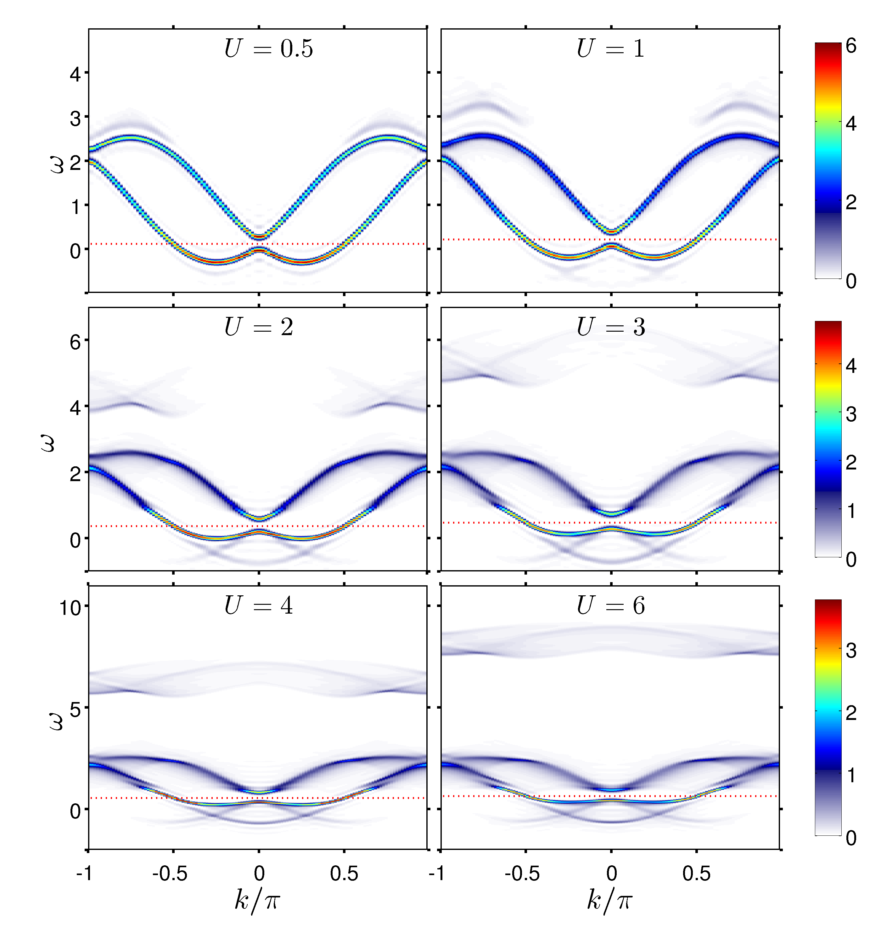
Figure 12: $S_{cc^{\dagger}}(k,\omega)$ for $n=0.5$, $\alpha=1$, $B=0.1$, $L=128$ and several values of $U$ ($U^{\prime}=0$). The dotted red line indicates the Fermi energy.

Appendix C Strong coupling region at incommensurate filling

In figure 13 we provide the spectral functions and structure factors for two different filling factors at a large value of $U=6$ in the strong coupling region. For both $n=0.41$ and $n=0.61$, the charge gap determined by Eq. (3.6) vanishes, although the spectral functions shown in figure 13 (a) exhibit a reduced spectral density around the Fermi level. The charge structure factor $S_{\hat{n}\hat{n}}(k,\omega)$ displayed in figure 13 (b) presents its largest contribution at $k=2k_{\text{F}}$ and $\omega=0$, indicating a tendency towards a charge density wave phase, while the spin structure factor shows a qualitatively similar behavior as for commensurate filling at smaller interactions.

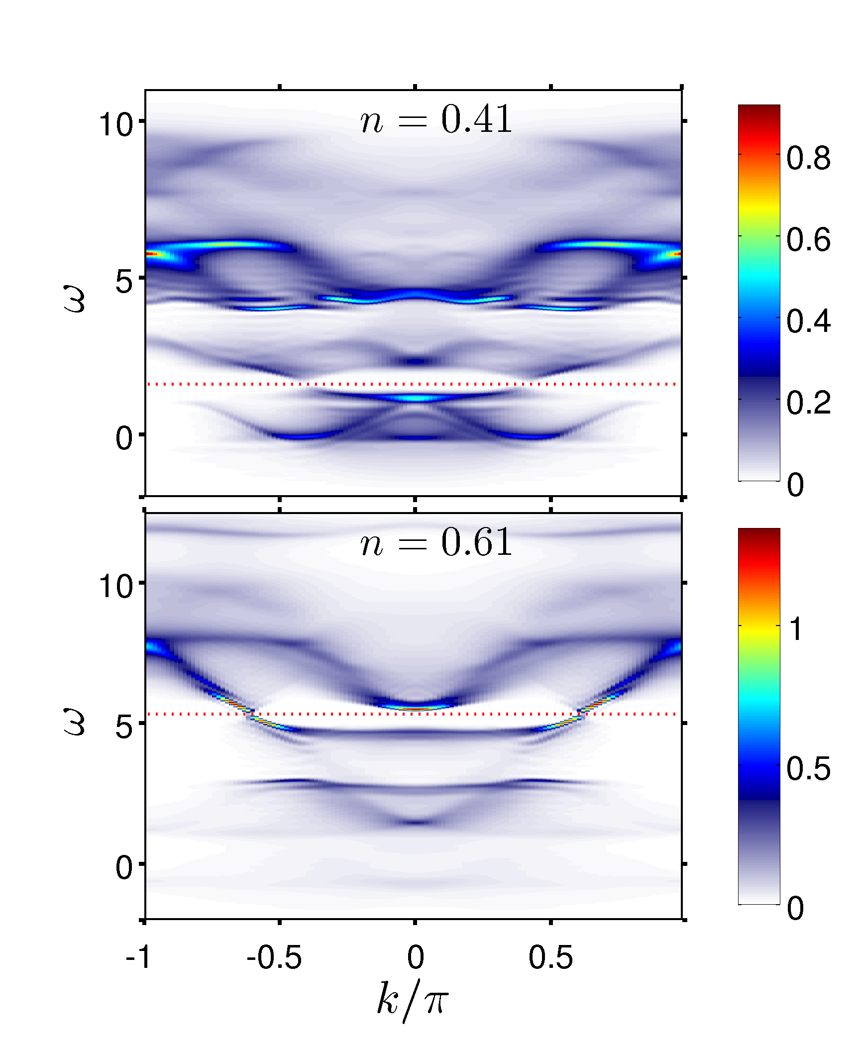
(a)

(b)

Figure 13: (a) Spectral functions and (b) charge and spin structure factors $S_{\hat{n}\hat{n}}(k,\omega)$ and $S_{\hat{S}^{y}\hat{S}^{y}}(k,\omega)$ for $n=0.41$ and $n=0.61$, with $\alpha=1$, $B=0.1$, $U=6$, $U^{\prime}=U/2$ and $L=128$.

References

- [1] Giamarchi T 2004 Quantum Physics in One Dimension (Clarendon Press)
- [2] Voit J 1995 Rep. Prog. Phys. 58 977
- [3] Meden V and Schönhammer K 1992 Phys. Rev. B 46 15753
- [4] Schönhammer K 2002 Journal of Physics: Condensed Matter 14 12783
- [5] Imambekov A and Glazman L I 2009 Science 323 228
- [6] Imambekov A, Schmidt T L and Glazman L I 2012 Rev. Mod. Phys. 84 1253–1306
- [7] White S R 1992 Phys. Rev. Lett. 69 2863
- [8] White S R 1993 Phys. Rev. B 48 10345
- [9] Manchon A, Koo H C, Nitta J, Frolov S M and Duine R A 2015 Nat Mater 14 871–882
- [10] Oreg Y, Refael G and von Oppen F 2010 Phys. Rev. Lett. 105 177002
- [11] Lutchyn R M, Sau J D and Das Sarma S 2010 Phys. Rev. Lett. 105 077001
- [12] Kitaev A 2003 Annals of Physics 303 2 – 30
- [13] Nayak C, Simon S H, Stern A, Freedman M and Das Sarma S 2008 Rev. Mod. Phys. 80(3) 1083–1159
- [14] Das A, Ronen Y, Most Y, Oreg Y, Heiblum M and Shtrikman H 2012 Nat Phys 8 887–895
- [15] Deng M T, Yu C L, Huang G Y, Larsson M, Caroff P and Xu H Q 2012 Nano Letters 12 6414–6419
- [16] Mourik V, Zuo K, Frolov S M, Plissard S R, Bakkers E P A M and Kouwenhoven L P 2012 Science 336 1003–1007
- [17] Albrecht S M, Higginbotham A P, Madsen M, Kuemmeth F, Jespersen T S, Nygård J, Krogstrup P and Marcus C M 2016 Nature 531 206–209
- [18] Quay C H L, Hughes T L, Sulpizio J A, Pfeiffer L N, Baldwin K W, West K W, Goldhaber-Gordon D and de Picciotto R 2010 Nat. Phys. 6 336
- [19] Heedt S, Traverso Ziani N, Crepin F, Prost W, Trellenkamp S, Schubert J, Grutzmacher D, Trauzettel B and Schapers T 2017 Nat Phys advance online publication –
- [20] Birkholz J 2008 Spin-orbit Interaction in Quantum Dots and Quantum Wires of Correlated Electrons - A Way to Spintronics? Ph.D. thesis Universität Göttingen
- [21] Středa P and Šeba P 2003 Phys. Rev. Lett. 90 256601
- [22] Mazza F, Braunecker B, Recher P and Levy Yeyati A 2013 Phys. Rev. B 88 195403
- [23] Sato K, Loss D and Tserkovnyak Y 2010 Phys. Rev. Lett. 105 226401
- [24] Cheuk L W, Sommer A T, Hadzibabic Z, Yefsah T, Bakr W S and Zwierlein M W 2012 Phys. Rev. Lett. 109 095302
- [25] Wang P, Yu Z Q, Fu Z, Miao J, Huang L, Chai S, Zhai H and Zhang J 2012 Phys. Rev. Lett. 109 095301
- [26] Schulz A, De Martino A, Ingenhoven P and Egger R 2009 Phys. Rev. B 79 205432
- [27] Japaridze G I, Johannesson H and Ferraz A 2009 Phys. Rev. B 80(4) 041308
- [28] Schulz A, De Martino A and Egger R 2010 Phys. Rev. B 82(3) 033407
- [29] Malard M, Grusha I, Japaridze G I and Johannesson H 2011 Phys. Rev. B 84(7) 075466
- [30] Thakurathi M, Loss D and Klinovaja J 2016 ArXiv 1608.08143
- [31] Schmidt T L and Pedder C J 2016 Phys. Rev. B 94(12) 125420
- [32] Pedder C J, Meng T, Tiwari R P and Schmidt T L 2016 Phys. Rev. B 94(24) 245414
- [33] Governale M and Zülicke U 2002 Phys. Rev. B 66(7) 073311
- [34] Gambetta F M, Ziani N T, Barbarino S, Cavaliere F and Sassetti M 2015 Phys. Rev. B 91(23) 235421
- [35] Gangadharaiah S, Sun J and Starykh O A 2008 Phys. Rev. B 78 054436
- [36] Governale M and Zülicke U 2004 Solid State Communications 131 581 – 589
- [37] Gritsev V, Japaridze G, Pletyukhov M and Baeriswyl D 2005 Phys. Rev. Lett. 94(13) 137207
- [38] Braunecker B, Simon P and Loss D 2009 Phys. Rev. Lett. 102 116403
- [39] Braunecker B, Simon P and Loss D 2009 Phys. Rev. B 80 165119
- [40] Braunecker B, Japaridze G I, Klinovaja J and Loss D 2010 Phys. Rev. B 82 045127
- [41] Braunecker B, Bena C and Simon P 2012 Phys. Rev. B 85 035136
- [42] Schuricht D 2012 Phys. Rev. B 85 121101(R)
- [43] Meng T, Fritz L, Schuricht D and Loss D 2014 Phys. Rev. B 89 045111
- [44] Scheller C P, Liu T M, Barak G, Yacoby A, Pfeiffer L N, West K W and Zumbühl D M 2014 Phys. Rev. Lett. 112(6) 066801
- [45] Glazov M M and Sherman E Y 2011 Phys. Rev. Lett. 107(15) 156602
- [46] Bindel J R, Pezzotta M, Ulrich J, Liebmann M, Sherman E Y and Morgenstern M 2016 Nat Phys 12 920–925
- [47] van Weperen I, Tarasinski B, Eeltink D, Pribiag V S, Plissard S R, Bakkers E P A M, Kouwenhoven L P and Wimmer M 2015 Phys. Rev. B 91(20) 201413
- [48] Stoudenmire E M, Alicea J, Starykh O A and Fisher M P 2011 Phys. Rev. B 84 014503
- [49] Kitaev A Y 2001 Physics-Uspekhi 44 131
- [50] Calvanese Strinati M, Cornfeld E, Rossini D, Barbarino S, Dalmonte M, Fazio R, Sela E and Mazza L 2016 ArXiv 1612.06682
- [51] Barbarino S, Taddia L, Rossini D, Mazza L and Fazio R 2016 New Journal of Physics 18 035010
- [52] Barbarino S, Taddia L, Rossini D, Mazza L and Fazio R 2015 Nature Communications 6 8134
- [53] Andergassen S, Enss T, Meden V, Metzner W, Schollwöck U and Schönhammer K 2006 Phys. Rev. B 73 045125
- [54] Fannes M, Nachtergaele B and Werner R F 1992 Comm. Math. Phys. 144 443–490
- [55] Schollwöck U 2011 Annals of Physics 326 96
- [56] Weiße A, Wellein G, Alvermann A and Fehske H 2006 Rev. Mod. Phys. 78(1) 275–306
- [57] Holzner A, Weichselbaum A, McCulloch I P, Schollwöck U and von Delft J 2011 Phys. Rev. B 83 195115
- [58] Thomale R, Rachel S and Schmitteckert P 2013 Phys. Rev. B 88(16) 161103
- [59] Braun A and Schmitteckert P 2014 Phys. Rev. B 90(16) 165112
- [60] Ganahl M, Thunström P, Verstraete F, Held K and Evertz H G 2014 Phys. Rev. B 90 045144
- [61] Wolf F A, Justiniano J A, McCulloch I P and Schollwöck U 2015 Phys. Rev. B 91(11) 115144
- [62] Dargel P E, Wöllert A, Honecker A, McCulloch I P, Schollwöck U and Pruschke T 2012 Phys. Rev. B 85 205119
- [63] Nocera A and Alvarez G 2016 Phys. Rev. E 94(5) 053308
- [64] Vidal G 2003 Phys. Rev. Lett. 91 147902
- [65] Vidal G 2004 Phys. Rev. Lett. 93 040502
- [66] White S R and Affleck I 2008 Phys. Rev. B 77 134437
- [67] Barthel T, Schollwöck U and White S R 2009 Phys. Rev. B 79 245101
- [68] Ganahl M, Aichhorn M, Thunström P, Held K, Evertz H G and Verstraete F 2015 Phys. Rev. B 92 155132
- [69] Seabra L, Essler F H L, Pollmann F, Schneider I and Veness T 2014 Phys. Rev. B 90(24) 245127
- [70] Assaad F and Evertz H 2008 World-line and Determinantal Quantum Monte Carlo Methods for Spins, Phonons and Electrons (Lecture Notes in Physics vol 739) (Springer Berlin Heidelberg)
- [71] Jeckelmann E 2002 Phys. Rev. B 66 045114
- [72] Kühner T D and White S R 1999 Phys. Rev. B 60 335
- [73] Zamolodchikov A B 1995 International Journal of Modern Physics A 10 1125
- [74] Maier F, Meng T and Loss D 2014 Phys. Rev. B 90 155437
- [75] Mila F and Zotos X 1993 Europhysics Letters 24 133
- [76] Essler F H L and Tsvelik A M 2002 Phys. Rev. B 65 115117
- [77] Essler F H L and Tsvelik A M 2003 Phys. Rev. Lett. 90(12) 126401
- [78] Benthien H, Gebhard F and Jeckelmann E 2004 Phys. Rev. Lett. 92 256401
- [79] Schmidt T L, Imambekov A and Glazman L I 2010 Phys. Rev. Lett. 104 116403
- [80] Ejima S, Gebhard F and Nishimoto S 2005 Europhysics Letters 70 492
- [81] Sela E, Altland A and Rosch A 2011 Phys. Rev. B 84(8) 085114
- [82] Hassler F and Schuricht D 2012 New Journal of Physics 14 125018
- [83] Schönhammer K, Meden V, Metzner W, Schollwöck U and Gunnarsson O 2000 Phys. Rev. B 61 4393
- [84] Meden V, Metzner W, Schollwöck U, Schneider O, Stauber T and Schönhammer K 2000 The European Physical Journal B - Condensed Matter and Complex Systems 16 631–646
- [85] Essler F H L and Konik R M 2005 From Fields to Strings: Circumnavigating Theoretical Physics (World Scientific, Singapore)
- [86] Gogolin A, Nersesyan A and Tsvelik A 2004 Bosonization and Strongly Correlated Systems (Cambridge University Press)
- [87] Pereira R G and Sela E 2010 Phys. Rev. B 82 115324
- [88] Ejima S and Fehske H 2010 Journal of Physics: Conference Series 200 012031
- [89] Karrasch C, Kennes D M and Moore J E 2014 Phys. Rev. B 90 155104
- [90] Oreg Y, Sela E and Stern A 2014 Phys. Rev. B 89(11) 115402
- [91] Cornfeld E, Neder I and Sela E 2015 Phys. Rev. B 91(11) 115427
- [92] Cornfeld E and Sela E 2015 Phys. Rev. B 92(11) 115446
- [93] Cavaliere F, Gambetta F M, Barbarino S and Sassetti M 2015 Phys. Rev. B 92(23) 235128
- [94] Press W H, Teukolsky S A and Vetterling WT Flannery B P 2007 Numerical Recipes in C, 3rd edition (Cambridge University Press)
- [95] Goth F and Assaad F F 2014 Phys. Rev. B 90 195103