Candidates for Universal Measures of Multipartite Entanglement

Abstract

We propose and examine several candidates for universal multipartite entanglement measures. The most promising candidate for applications needing entanglement in the full Hilbert space is the ent-concurrence, which detects all entanglement correlations while distinguishing between different types of distinctly multipartite entanglement, and simplifies to the concurrence for two-qubit mixed states. For applications where subsystems need internal entanglement, we develop the absolute ent-concurrence which detects the entanglement in the reduced states as well as the full state.

I Introduction

\begin{picture}(100.0,0.0)\put(1.0,24.0){\hypertarget{Sec:I}{}} \end{picture}

Entanglement Einstein et al. (1935); Schrödinger (1935), in the simplest case of pure quantum states, is when a state such as $|\psi\rangle=a|1\rangle\otimes|1\rangle+b|1\rangle\otimes|2\rangle+c|2\rangle\otimes|1\rangle+d|2\rangle\otimes|2\rangle$, where $|a|^{2}+|b|^{2}+|c|^{2}+|d|^{2}=1$, cannot be factored as a tensor product of pure states such as $|\psi\rangle\!=\!(w|1\rangle\!+\!{\kern 1.0pt}x|2\rangle)\otimes(y|1\rangle\!+\!{\kern 1.0pt}z|2\rangle)$, where $|w|^{2}+|x|^{2}=1$ and $|y|^{2}+|z|^{2}=1$, where we have expressed each qubit in a generic basis $\{|1\rangle,|2\rangle\}$ (our convention in this paper, and these kets do not imply Fock states Dirac (1927)).

Quantum mixed states are $\rho\equiv\sum\nolimits_{j}p_{j}|\psi_{j}\rangle\langle\psi_{j}|$, where $p_{j}\in[0,1]$, $\sum\nolimits_{\textnormal{\raisebox{1.0pt}[1.0pt][1.0pt]{$j$}}}p_{j}=1$, and all $|\psi_{j}\rangle$ are pure. For bipartite systems, those composed of two subsystems (modes), mixed states $\varsigma\equiv\varsigma^{(1,2)}$ are separable if and only iff (iff)

$$\varsigma^{(1,2)}=\sum\nolimits_{j}{p_{j}\varsigma_{j}^{(1)}\otimes\varsigma_{j}^{(2)}},$$ (1)

where parenthetical superscripts are mode labels, and each $\varsigma_{j}^{\textnormal{\raisebox{0.0pt}[0.0pt][0.0pt]{${\kern 1.5pt}(m)$}}}$ is pure. Each mode-$m$ reduced state ${\varsigma}{\kern-5.3pt}{{\textnormal{\raisebox{-1.2pt}{\scalebox{1.2}{\textasciicaron}}}}}{\kern-4.2pt}{~{}}^{(m)}\!\equiv\!\text{tr}_{{\kern 0.0pt}\mathop{m}\limits^{{\kern-0.3pt}{\overline{{\kern 5.5pt}}}}{\kern 0.0pt}}(\varsigma)$, where $\mathop{m}\limits^{{\kern-3.5pt}~{}_{\overline{{\kern 7.0pt}}}}$ means “not $m$” (see App.A), admits a decomposition of the form ${\varsigma}{\kern-5.3pt}{{\textnormal{\raisebox{-1.2pt}{\scalebox{1.2}{\textasciicaron}}}}}{\kern-4.2pt}{~{}}^{(m)}\equiv\sum\nolimits_{\textnormal{\raisebox{1.0pt}[1.0pt][1.0pt]{$j$}}}{p_{j}{\varsigma}{\kern-5.3pt}{{\textnormal{\raisebox{-1.2pt}{\scalebox{1.2}{\textasciicaron}}}}}{\kern-4.2pt}{~{}}^{{\kern 0.5pt}\textnormal{\raisebox{0.0pt}[0.0pt][0.0pt]{$(m)$}}}_{{\kern-2.0pt}j}}$ $=\!\sum\nolimits_{\textnormal{\raisebox{1.0pt}[1.0pt][1.0pt]{$j$}}}{p_{j}\varsigma_{j}^{\textnormal{\raisebox{0.0pt}[0.0pt][0.0pt]{${\kern 1.5pt}(m)$}}}}$ as proved in App.B, so if we only knew reductions ${\varsigma}{\kern-5.3pt}{{\textnormal{\raisebox{-1.2pt}{\scalebox{1.2}{\textasciicaron}}}}}{\kern-4.2pt}{~{}}^{(m)}$, we could search decompositions of each one to find the pair with matching sets $\{p_{j}\}$ such that $\varsigma^{(1,2)}\!=\!\sum\nolimits_{\textnormal{\raisebox{1.0pt}[1.0pt][1.0pt]{$j$}}}{p_{j}{\varsigma}{\kern-5.3pt}{{\textnormal{\raisebox{-1.2pt}{\scalebox{1.2}{\textasciicaron}}}}}{\kern-4.2pt}{~{}}^{{\kern 0.5pt}\textnormal{\raisebox{0.0pt}[0.0pt][0.0pt]{$(1)$}}}_{{\kern-2.0pt}j}\otimes{\varsigma}{\kern-5.3pt}{{\textnormal{\raisebox{-1.2pt}{\scalebox{1.2}{\textasciicaron}}}}}{\kern-4.2pt}{~{}}^{{\kern 0.5pt}\textnormal{\raisebox{0.0pt}[0.0pt][0.0pt]{$(2)$}}}_{{\kern-2.0pt}j}}$. Therefore knowledge of the reductions allows reconstruction of the parent state $\varsigma$.

For $N$-partite ($N$-mode) systems, separability can occur in more than one way. For example, two different $3$-qubit pure states could have separable bipartitions as $\rho={\rho}{\kern-5.3pt}{{\textnormal{\raisebox{-1.2pt}{\scalebox{1.2}{\textasciicaron}}}}}{\kern-4.2pt}{~{}}^{(1)}\otimes{\rho}{\kern-5.3pt}{{\textnormal{\raisebox{-1.2pt}{\scalebox{1.2}{\textasciicaron}}}}}{\kern-4.2pt}{~{}}^{(2,3)}$ and $\varrho={\varrho}{\kern-5.3pt}{{\textnormal{\raisebox{-1.2pt}{\scalebox{1.2}{\textasciicaron}}}}}{\kern-4.2pt}{~{}}^{(1,2)}\otimes{\varrho}{\kern-5.3pt}{{\textnormal{\raisebox{-1.2pt}{\scalebox{1.2}{\textasciicaron}}}}}{\kern-4.2pt}{~{}}^{(3)}$, so we call both of them biseparable or $2$-separable, even though the mode groups that are separable for each state are different.

These different mode-groupings are called partitions, which are definitions of new modes composed of (but not subdividing) the original modes $m_{k}$, as explained in App.C. For example, a tripartite state like $\rho^{(1,2,3)}$ can have three unique bipartitions $\rho^{(1|2,3)},\rho^{(2|1,3)},\rho^{(3|1,2)}$ and one unique tripartition $\rho^{(1|2|3)}=\rho^{(1,2,3)}$, showing that in the absence of partitions, the commas are the partitions.

To handle the general $N$-partite phenomenon of separability of a given partitioning having the potential to occur in different ways, the notion of $k$-separability was developed Huber et al. (2011); Ma et al. (2011); Huber et al. (2010); Coffman et al. (2000); Horodecki et al. (2001); Plenio and Vedral (2001); Eisert and Briegel (2001); Meyer and Wallach (2002); Seevinck and Svetlichny (2002); Miyake (2003); Wocjan and Horodecki (2005); Yu and Song (2005); Lohmayer et al. (2006); Hassan and Joag (2008), as depicted in Fig.1.

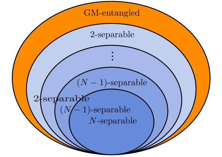
Figure 1: (color online) Relationships of $k$-separabilities Huber et al. (2011). Each $k$-separability implies all lower-$k$-separabilities, and is necessary for all higher-$k$-separabilities. Thus, $N$-separable states are also $(N-1)$-separable, all the way down to $2$-separable, but some $2$-separable states are not $3$-separable or higher. The “1-separable” states are “genuinely multipartite (GM) entangled,” also defined as all states that are not $2$-separable. Thus, the GM-entangled region is strictly crescent-shaped here, while the $k$-separable regions are each ellipse-shaped and coinciding with parts of all lower-$k$-separabilities. (The shapes are arbitrary, merely representing relationships.)

By definition, $k$-separability of pure states is when any member of the set of all possible $k$-partitions has $k$-mode product form, for a fixed $k$. Thus, for a pure $\rho^{(1,2,3)}$, if only $\rho^{(2|1,3)}$ is $2$-separable, but not $\rho^{(1|2,3)}$ or $\rho^{(3|1,2)}$, then that is sufficient for $\rho^{(1,2,3)}$ to be $2$-separable.

Mixed states are $k$-separable if a decomposition exists for which all pure decomposition states are at least $k$-separable, with one being exactly $k$-separable Huber et al. (2011) (since higher-than-$k$-separabilities are also $k$-separable, we can just say that all decomposition states need to be $k$-separable). For example, the $3$-qudit state

$$\begin{array}[]{*{20}l}{\rho}&\!\!{=\sum\limits_{j}{{\kern-1.0pt}p_{j}\rho_{j}^{(1)}\!\otimes{\kern-1.0pt}\rho_{j}^{(2,3)}}\!+\!\sum\limits_{k}{{\kern-1.0pt}q_{k}\rho_{k}^{(2)}\!\otimes{\kern-1.0pt}\rho_{k}^{(1,3)}}\!+\!\sum\limits_{l}{{\kern-1.0pt}r_{l}\rho_{l}^{(3)}\!\otimes{\kern-1.0pt}\rho_{l}^{(1,2)}}\!,}\\ \end{array}$$ (2)

where $p_{j},q_{k},r_{l}\in[0,1]$, $(\sum\nolimits_{j}{p_{j}})\!+\!(\sum\nolimits_{k}{q_{k}})\!+\!(\sum\nolimits_{l}{r_{l}})=1$, with pure entangled bipartite states $\rho_{{\kern-0.3pt}j}^{\textnormal{\raisebox{-1.0pt}[-1.0pt][-1.0pt]{${\kern 2.0pt}(2,3)$}}},\rho_{{\kern-0.3pt}k}^{\textnormal{\raisebox{-1.0pt}[-1.0pt][-1.0pt]{${\kern 2.0pt}(1,3)$}}},\rho_{{\kern-0.3pt}l}^{\textnormal{\raisebox{-1.0pt}[-1.0pt][-1.0pt]{${\kern 2.0pt}(1,2)$}}}$ and pure $\rho_{{\kern-0.5pt}\textnormal{\raisebox{0.5pt}[0.5pt][0.5pt]{$j$}}}^{{\kern 1.5pt}\textnormal{\raisebox{0.5pt}[0.5pt][0.5pt]{$(1)$}}},\rho_{k}^{{\kern 1.5pt}\textnormal{\raisebox{0.5pt}[0.5pt][0.5pt]{$(2)$}}},\rho_{l}^{{\kern 1.5pt}\textnormal{\raisebox{0.5pt}[0.5pt][0.5pt]{$(3)$}}}$, is $2$-separable (biseparable), even though each group of pure decomposition states is separable over different bipartitions Huber et al. (2011).

Here, we define the “absence of $k$-separability” (meaning no $k$-partitions of a pure state have $k$-partite product form) as full $k$-partite entanglement ($\text{F}_{k}$-entanglement) for $k{\kern-2.0pt}>{\kern-2.0pt}1$ as shown in Fig.2, found by combining entanglement values (by some measure) over all $k$-partitions, and named in analogy to “full $N$-partite entanglement” being the absence of full $N$-partite separability. However, the absence of $2$-separability is also “$2$-entanglement,” known as “genuinely multipartite (GM) entanglement.” We use the term GM-$k$-entanglement ($\text{GM}_{k}$-entanglement) in lieu of the traditional term “$k$-entanglement” as the minimum entanglement over all $k$-partitions.

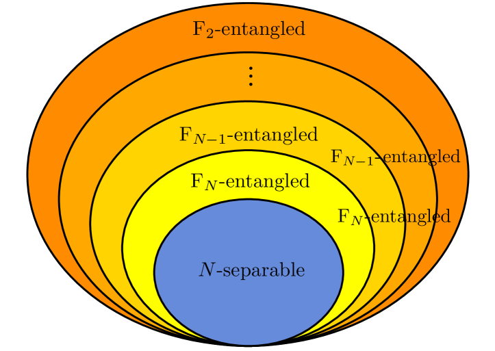
Figure 2: (color online) Relationships of $\text{F}_{k}$-entanglements. Here, a given $\text{F}_{k}$-entanglement implies all higher-$k$ $\text{F}_{k}$-entanglements, while being itself necessary for all lower-$k$ $\text{F}_{k}$-entanglements. Thus, each $\text{F}_{k}$-entanglement region is strictly crescent-shaped and coinciding with parts of all higher-$k$ $\text{F}_{k}$-entanglements, with $\text{F}_{N}$-entanglement being the thickest crescent, and all lower-$k$ $\text{F}_{k}$-entanglements having progressively thinner crescents. The entire region that is not $N$-separable is $\text{F}_{N}$-entangled.

On the other hand, $N$-partite states are entangled iff they are $\text{F}_{N}$-entangled, as proved in App.D. This means that the complete absence of entanglement correlations can only occur in $N$-partite states that are $N$-separable, meaning states with an optimal decomposition,

$$\varsigma^{(1,\ldots,N)}{\kern-1.0pt}={\kern-2.0pt}\sum\nolimits_{j}{{\kern-1.0pt}p_{j}{\kern-2.0pt}\mathop{\otimes}\limits_{m=1}^{N}{\kern-2.0pt}\varsigma_{j}^{(m)}}{\kern-1.0pt}={\kern-2.0pt}\sum\nolimits_{j}{{\kern-1.0pt}p_{j}\varsigma_{j}^{(1)}{\kern-2.0pt}\otimes\cdots\otimes\varsigma_{j}^{(N)}}{\kern-2.0pt},$$ (3)

where the $\varsigma_{j}^{(m)}$ are pure. $N$-partite states that cannot be expanded as (3) are full $N$-partite entangled ($\text{F}_{N}$-entangled). We will often say entanglement correlation instead of just entanglement to remind that there are other kinds of nonlocal correlation not involving entanglement.

However, $\text{F}_{N}$-entanglement cannot distinguish between types of multipartite entanglement. For example, given

$$\rho_{|\Phi_{\text{GHZ}}\rangle}\;\;\;\text{and}\;\;\;\rho_{|\Phi_{\text{BP}}\rangle}\equiv\rho_{|\Phi^{+}\rangle}\otimes\rho_{|\Phi^{+}\rangle},$$ (4)

where $|\Phi_{\textnormal{\raisebox{0.5pt}[0.5pt][0.5pt]{$\text{GHZ}$}}}\rangle\!\equiv\!\textnormal{\raisebox{1.0pt}[1.0pt][1.0pt]{$\textstyle{1\over{\sqrt{2}}}$}}(|1,\!1,\!1,\!1\rangle\!+\!|2,\!2,\!2,\!2\rangle)$ is a $4$-qubit GHZ state Greenberger et al. (1989, 1990); Mermin (1990) where $\rho_{\textnormal{\raisebox{0.5pt}[0.5pt][0.5pt]{$|A\rangle$}}}\!\equiv\!|A\rangle\langle A|$, and $|\Phi^{+}\rangle\!\equiv\!\textnormal{\raisebox{1.0pt}[1.0pt][1.0pt]{$\textstyle{1\over{\sqrt{2}}}$}}(|1,1\rangle+$ $|2,2\rangle)$ is a $2$-qubit Bell state so that $\rho_{|\Phi_{\text{BP}}\rangle}$ is a “Bell-product state,” since both $\rho_{|\Phi_{\text{GHZ}}\rangle}$ and $\rho_{|\Phi_{\text{BP}}\rangle}$ have maximal mixing in all single-mode reductions, an $\text{F}_{N}$-entanglement measure would report both states as being equally entangled, despite $\rho_{|\Phi_{\text{GHZ}}\rangle}$ being $\text{F}_{2}$-entangled and $\text{GM}_{2}$-entangled while $\rho_{|\Phi_{\text{BP}}\rangle}$ is $2$-separable.

Yet, $\text{GM}_{2}$-entanglement alone cannot detect the strong entanglement correlations within the Bell states of $\rho_{|\Phi_{\text{BP}}\rangle}$ in (4). Thus, while $\text{F}_{N}$-entanglement can detect the presence of all entanglement correlations but cannot distinguish $k$-separabilities, lone sub-$N$ $\text{GM}_{k}$-entanglement measures are not sufficient to detect the presence of all entanglement correlations, but can verify $k$-separability.

Therefore our main goal here is to define a few candidate universal entanglement measures that distinguish between types of multipartite entanglement without discarding information about entanglement correlations, which individual $\text{GM}_{k}$-entanglement measures cannot do alone.

The building-block of our candidate measures is the $\text{F}_{N}$-entanglement measure the ent Hedemann (2016), given by

$$\Upsilon(\rho)\equiv{\kern-1.0pt}\Upsilon(\rho,\mathbf{n}){\kern-1.0pt}\equiv{\kern-1.0pt}\frac{1}{M(L_{*})}{\kern-1.0pt}\left({\kern-1.0pt}{1-\frac{1}{N}\sum\limits_{m=1}^{N}\!{\frac{{n_{m}P({\rho}{\kern-5.3pt}{{\textnormal{\raisebox{-1.2pt}{\scalebox{1.2}{\textasciicaron}}}}}{\kern-4.2pt}{~{}}^{(m)})-1}}{{n_{m}-1}}}}{\kern-1.0pt}\right)\!,$$ (5)

for pure states $\rho$ of an $N$-mode $n$-level system where mode $m$ has $n_{m}$ levels and $\mathbf{n}\equiv(n_{1},\ldots,n_{N})$, so that $n=n_{1}\cdots n_{N}=\text{det}(\text{diag}(\mathbf{n}))$, $N=\text{dim}(\mathbf{n})$, $P(\sigma)\equiv\text{tr}(\sigma^{2})$ is the purity of $\sigma$, and ${\rho}{\kern-5.3pt}{{\textnormal{\raisebox{-1.2pt}{\scalebox{1.2}{\textasciicaron}}}}}{\kern-4.2pt}{~{}}^{(m)}$ is the $n_{m}$-level single-mode reduction of $\rho$ for mode $m$ (see App.A). The normalization factor $M(L_{*})\equiv M(L_{*},\mathbf{n})$ is given in App.E. Basically, the ent measures how simultaneously mixed the ${\rho}{\kern-5.3pt}{{\textnormal{\raisebox{-1.2pt}{\scalebox{1.2}{\textasciicaron}}}}}{\kern-4.2pt}{~{}}^{(m)}$ are.

We will also use the partitional ent $\Upsilon^{(\mathbf{m}^{\textnormal{\raisebox{-1.0pt}[-1.0pt][-1.0pt]{$(\mathbf{T})$}}})}(\rho)\equiv$ $\Upsilon({\rho}{\kern-5.3pt}{{\textnormal{\raisebox{-1.2pt}{\scalebox{1.2}{\textasciicaron}}}}}{\kern-4.2pt}{~{}}^{(\mathbf{m})},\mathbf{n}^{(\mathbf{m}^{\textnormal{\raisebox{-1.0pt}[-1.0pt][-1.0pt]{$(\mathbf{T})$}}})})$, allowing us to repartition $\rho$’s reduction ${\rho}{\kern-5.3pt}{{\textnormal{\raisebox{-1.2pt}{\scalebox{1.2}{\textasciicaron}}}}}{\kern-4.2pt}{~{}}^{(\mathbf{m})}$ (including the nonreduction ${\rho}{\kern-5.3pt}{{\textnormal{\raisebox{-1.2pt}{\scalebox{1.2}{\textasciicaron}}}}}{\kern-4.2pt}{~{}}^{(\mathbf{N})}\equiv{\rho}{\kern-5.3pt}{{\textnormal{\raisebox{-1.2pt}{\scalebox{1.2}{\textasciicaron}}}}}{\kern-4.2pt}{~{}}^{(1,\ldots,N)}=\rho$) into new mode groups $\mathbf{m}^{(\mathbf{T})}\equiv(\mathbf{m}^{(1)}|\ldots|\mathbf{m}^{(T)})$ of levels $\mathbf{n}^{(\mathbf{m}^{\textnormal{\raisebox{-1.0pt}[-1.0pt][-1.0pt]{$(\mathbf{T})$}}})}\equiv(n_{\mathbf{m}^{(1)}},\ldots,n_{\mathbf{m}^{(T)}})$ (see App.C) to measure the $\text{F}_{T}$-entanglement of any $T$ mode groups (see Hedemann (2016) for details). Finally, when $\rho$ or ${\rho}{\kern-5.3pt}{{\textnormal{\raisebox{-1.2pt}{\scalebox{1.2}{\textasciicaron}}}}}{\kern-4.2pt}{~{}}^{(\mathbf{m})}$ are mixed, we use convex-roof extensions as $\hat{\Upsilon}$ and $\hat{\Upsilon}^{(\mathbf{m}^{\textnormal{\raisebox{-1.0pt}[-1.0pt][-1.0pt]{$(\mathbf{T})$}}})}$ (see (Hedemann, 2016, App.J)), which are minimum average ents over all decompositions. The main sections of this paper are:

I.	Introduction. ​​	I
II.	Candidate Pure-State Entanglement Measures . ​​	II
III.	Tests of Candidate Pure-State Measures. ​​	III
IV.	Candidate Mixed-State Measures. ​​	IV
V.	Tests of Candidate Mixed-State Measures. ​​	V
VI.	Ent-Concurrence. ​​	VI
VII.	Absolute Ent-Concurrence. ​​	VII
VIII.	Conclusions. ​​	VIII
App.	Appendices. ​​	A
A.	Brief Review of Reduced States. ​​	A
B.	$N$-Separability of $N$-Partite States Implies Reconstructability by Smallest Reductions. ​​	B
C.	Definition of Partitions. ​​	C
D.	Proof that $N$-Partite States are Entangled If and Only If they are $\text{F}_{N}$-Entangled. ​​	D
E.	Normalization Factor of the Ent. ​​	E
F.	True-Generalized X (TGX) States. ​​	F
G.	Full Set of 4-Qubit Maximally $\text{F}_{N}$-Entangled TGX States Involving $|1\rangle$. ​​	G
H.	Quantum Mixed States Cannot Be Treated as Time-Averages of Varying Pure States. ​​	H

and wherever possible, details are put in the Appendices.

II Candidate Pure-State Entanglement Measures

\begin{picture}(100.0,0.0)\put(1.0,27.0){\hypertarget{Sec:II}{}} \end{picture}

Here we introduce the candidate entanglement measures under consideration. Each will use the ent from (5) as well as its various different forms due to partitioning. See Hedemann (2016) for full explanations. We start with pure-state measures, and discuss mixed input after initial tests.

II.1 Full Genuinely Multipartite (FGM) Ent

The FGM ent for pure $\rho$ is

$$\Upsilon_{\text{FGM}}(\rho)\equiv\frac{1}{M_{\text{FGM}}}\sum\limits_{k=2}^{N}{\Upsilon_{\text{GM}_{k}}(\rho)},$$ (6)

where $M_{\text{FGM}}$ is a normalization factor, and

$$\Upsilon_{\text{GM}_{k}}(\rho)\equiv\min(\{\Upsilon^{(\mathbf{N}_{h}^{(\mathbf{k})})}(\rho)\}),$$ (7)

which is the $\text{GM}_{k}$ ent, where $\{\Upsilon^{(\mathbf{N}_{h}^{(\mathbf{k})})}(\rho)\}$ is the set of all $N$-mode $k$-partitional ents, each labeled by $h$. Note that Hedemann (2016) defined the GM ent as $\Upsilon_{\text{GM}}(\rho)\equiv\Upsilon_{\text{GM}_{2}}(\rho)$, which is the “ent-version” of GM concurrence $C_{\text{GM}}(\rho)$ Ma et al. (2011).

Since $\Upsilon_{\text{FGM}}$ sums all $\text{GM}_{k}$ ents, it is a measure of simultaneous $\text{GM}_{k}$-entanglements; that is, it rates states for which the combination of all their $\text{GM}_{k}$-entanglements is maximal as being “maximally FGM-entangled.”

II.2 Full Simultaneously Multipartite (FSM) Ent

The FSM ent for pure $\rho$ is

$$\Upsilon_{\text{FSM}}(\rho)\equiv\frac{1}{M_{\text{FSM}}}\sum\limits_{k=2}^{N}{\Upsilon_{\text{SM}_{k}}(\rho)},$$ (8)

where $M_{\text{FSM}}$ is a normalization factor, and we define the simultaneously multipartite $k$-ent ($\text{SM}_{k}$ ent) as

$$\Upsilon_{\text{SM}_{k}}(\rho)\equiv\frac{1}{M_{\text{SM}_{k}}}\sum\nolimits_{h=1}^{\{_{\,k}^{N}\}}\Upsilon^{(\mathbf{N}_{h}^{(\mathbf{k})})}(\rho),$$ (9)

where $\{_{{\kern 1.0pt}k}^{N}\}\equiv\frac{1}{k!}\sum\nolimits_{{\kern 0.5pt}\textnormal{\raisebox{1.4pt}[1.4pt][1.4pt]{$j\!=\!0$}}}^{k}{\!(-1{\kern-0.5pt})^{k-j}\binom{k}{j}j^{N}}$ are Stirling numbers of the second kind, $\binom{\textnormal{\raisebox{-1.0pt}[-1.0pt][-1.0pt]{$k$}}}{\textnormal{\raisebox{1.0pt}[1.0pt][1.0pt]{$j$}}}{\kern-0.5pt}\equiv{\kern-0.5pt}\frac{k!}{j!(k-j)!}$, $\{\Upsilon^{\textnormal{\raisebox{-0.8pt}[-0.8pt][-0.8pt]{$(\mathbf{N}_{{\kern-0.5pt}\textnormal{\raisebox{-0.5pt}[-0.5pt][-0.5pt]{$h$}}}^{{\kern 0.5pt}\textnormal{\raisebox{-0.3pt}[-0.3pt][-0.3pt]{$(\mathbf{k})$}}})$}}}(\rho)\}$ is the set of all $N$-mode $k$-partitional ents, and $M_{\text{SM}_{k}}$ is a normalization factor. $\Upsilon_{\text{SM}_{k}}(\rho)$ detects the presence of any entanglement correlation among all possible $k$-partitions of $\rho$. Thus, it cannot ignore entanglement within particular $k$-partitions just because a different $k$-partition is separable as $\Upsilon_{\text{GM}_{k}}(\rho)$ can.

The FSM ent $\Upsilon_{\text{FSM}}$ is a measure of simultaneous $\text{SM}_{k}$ ents; which means it is a measure of the combination of all $N$-mode partitional ents, so it is a sum of all 2-partitional ents of $\rho$, all 3-partitional ents of $\rho$, all the way up to the $N$-partitional ent (the ent itself). Thus, if there is any entanglement correlation between any mode groups of $\rho$, the FSM will detect it, and states that maximize it are “maximally FSM-entangled.”

II.3 Full Distinguishably Multipartite (FDM) Ent: The Ent-Concurrence

The FDM ent (or the ent-concurrence) for pure $\rho$ is

$$\Upsilon_{\text{FDM}}(\rho)\equiv\frac{1}{M_{\text{FDM}}}\sum\limits_{k=2}^{N}{\Upsilon_{\text{DM}_{k}}(\rho)},$$ (10)

where $M_{\text{FDM}}$ is a normalization factor, and we define the distinguishably multipartite $k$-ent ($\text{DM}_{k}$ ent) as

$$\Upsilon_{\text{DM}_{k}}(\rho)\equiv\frac{1}{M_{\text{DM}_{k}}}\sum\nolimits_{h=1}^{\{_{\,k}^{N}\}}\sqrt{\Upsilon^{(\mathbf{N}_{h}^{(\mathbf{k})})}(\rho)},$$ (11)

where $M_{\text{DM}_{k}}$ is a normalization factor, $\{_{{\kern 1.0pt}k}^{N}\}$ are Stirling numbers of the second kind as in (9), and $\{\Upsilon^{\textnormal{\raisebox{-0.8pt}[-0.8pt][-0.8pt]{$(\mathbf{N}_{{\kern-0.4pt}\textnormal{\raisebox{-0.5pt}[-0.5pt][-0.5pt]{$h$}}}^{{\kern 0.5pt}\textnormal{\raisebox{-0.3pt}[-0.3pt][-0.3pt]{$(\mathbf{k})$}}})$}}}(\rho)\}$ is the set of all $N$-mode $k$-partitional ents.

The FDM ent $\Upsilon_{\text{FDM}}$ is a measure of simultaneous $\text{DM}_{k}$ ents $\Upsilon_{\text{DM}_{k}}$, and the $\Upsilon_{\text{DM}_{k}}$ measures not only the combination of all possible $N$-mode $k$-partitional ents, but also how equally distributed they are, rating states for which all $N$-mode $k$-partitional ents have the highest combination and are the most equal and numerous as having the highest $\text{DM}_{k}$ ent.

This is based on pseudonorm $|\mathbf{x}|_{1/2}\equiv\sum\nolimits_{k}\!\sqrt{x_{k}};\,x_{k}\geq 0$, which obeys $|\mathbf{x}|_{1/2}\!=\!0\Rightarrow\mathbf{x}\!=\!\mathbf{0}$ and the triangle inequality, and although $|a\mathbf{x}|_{1/2}\neq|a|\!\cdot\!|\mathbf{x}|_{1/2}$, that does not matter here, since our “vectors” are really just lists of scalars. The main reason we use this pseudonorm is because it rates an equally distributed $1$-norm-normalized vector such as $\mathbf{x}=(0.25,0.25,0.25,0.25)$ as having the highest “$\frac{1}{2}$-norm” value out of all vectors of the same $1$-norm, such as $\mathbf{y}=(0,0,0.5,0.5)$ or $\mathbf{z}=(0,1,0,0)$.

For two qubits ($N=2$), the FDM ent is the concurrence $C$ Hill and Wootters (1997); Wootters (1998), since $\Upsilon=C^{2}$ as proven in Hedemann (2016), so that

$$\Upsilon_{\text{FDM}}(\rho)=\Upsilon_{\text{DM}_{N}}(\rho)=\sqrt{\Upsilon(\rho)}=C(\rho),$$ (12)

(extendible to mixed states, as shown later). Therefore, if we let the $N$-mode $k$-partitional ent-concurrence be

$$C_{\Upsilon}^{(\mathbf{N}_{h}^{(\mathbf{k})})}(\rho)\equiv\sqrt{\Upsilon^{(\mathbf{N}_{h}^{(\mathbf{k})})}(\rho)},$$ (13)

where $\{\Upsilon^{(\mathbf{N}_{h}^{(\mathbf{k})})}(\rho)\}$ is the set of all $N$-mode $k$-partitional ents, then the $\text{DM}_{k}$ ent $\Upsilon_{\text{DM}_{k}}$ is simply a $1$-norm of all $\{C_{{\kern-1.0pt}\textnormal{\raisebox{-0.9pt}[-0.9pt][-0.9pt]{$\textnormal{\scalebox{0.85}{$\Upsilon$}}$}}}^{{\kern 0.0pt}\textnormal{\raisebox{-0.4pt}[-0.4pt][-0.4pt]{$(\mathbf{N}_{{\kern-0.5pt}h}^{{\kern 0.5pt}\textnormal{\raisebox{-0.3pt}[-0.3pt][-0.3pt]{$(\mathbf{k})$}}})$}}}(\rho)\}$ for a given $k$. Therefore, the $\Upsilon_{\text{FDM}}$ in (10) can also be called the ent-concurrence $C_{\Upsilon}$ for pure states.

III Tests of Candidate Pure-State Measures

\begin{picture}(100.0,0.0)\put(1.0,27.0){\hypertarget{Sec:III}{}} \end{picture}

For simple tests, we use $4$-qubit ($2\times 2\times 2\times 2$) states,

$$\begin{array}[]{*{20}l}{|\Phi_{\text{GHZ}}\rangle}&\!\!{\equiv{\textstyle{1\over{\sqrt{2}}}}(|1,\!1,\!1,\!1\rangle\!+\!|2,\!2,\!2,\!2\rangle)}\\ {|\Phi_{\text{BP}}\rangle}&\!\!{\equiv\rule{0.0pt}{8.5pt}{\textstyle{1\over{\sqrt{4}}}}(|1,\!1,\!1,\!1\rangle\!+\!|1,\!1,\!2,\!2\rangle\!+\!|2,\!2,\!1,\!1\rangle\!+\!|2,\!2,\!2,\!2\rangle)}\\ {|\Phi_{\text{F}}\rangle}&\!\!{\equiv\rule{0.0pt}{8.5pt}{\textstyle{1\over{\sqrt{4}}}}(|1,\!1,\!1,\!1\rangle\!+\!|1,\!1,\!2,\!2\rangle\!+\!|2,\!2,\!1,\!2\rangle\!+\!|2,\!2,\!2,\!1\rangle)}\\ {|\psi_{\text{W}}\rangle}&\!\!{\equiv\rule{0.0pt}{8.5pt}{\textstyle{1\over{\sqrt{4}}}}(|1,\!1,\!1,\!2\rangle\!+\!|1,\!1,\!2,\!1\rangle\!+\!|1,\!2,\!1,\!1\rangle\!+\!|2,\!1,\!1,\!1\rangle)}\\ {|\psi_{\text{Rand}}\rangle}&\!\!{\equiv\rule{0.0pt}{8.5pt}\sum\nolimits_{k=1}^{16}{a_{k}|k\rangle};\;\;\sum\nolimits_{k=1}^{16}{|a_{k}|^{2}}=1},\\ \end{array}$$ (14)

where $|\Phi_{\text{BP}}\rangle\!\equiv\!|\Phi^{+}\rangle\otimes|\Phi^{+}\rangle$ is the Bell product from (4), $|\psi_{\text{W}}\rangle$ is the W state Dür et al. (2000), and $|\psi_{\text{Rand}}\rangle$ is a random $16$-level pure state, where here and throughout we use basis abbreviation $\{|1\rangle,|2\rangle,\ldots,|n\rangle\}\equiv\{|1,\!1,\!1,\!1\rangle,$ $|1,\!1,\!1,\!2\rangle,\ldots,|2,\!2,\!2,\!2\rangle\}$. The states $|\Phi_{\text{GHZ}}\rangle$, $|\Phi_{\text{BP}}\rangle$, and $|\Phi_{\text{F}}\rangle$ are taken from the set of maximally $\text{F}_{N}$-entangled true-generalized X (TGX) states (see App.F, (Hedemann, 2016, App.D), and Hedemann (2013)), chosen from the subset including $|1\rangle$, generated by the 13-step algorithm of Hedemann (2016). Thus, (14) provides three maximally $\text{F}_{N}$-entangled states and two other kinds of states for comparison.

The subset $\{|\Phi_{\text{GHZ}}\rangle,|\Phi_{\text{BP}}\rangle,|\Phi_{\text{F}}\rangle\}$ was chosen from the full set of $\text{F}_{N}$-entangled TGX states since they produced distinct results for the measures under test and included $|\Phi_{\text{GHZ}}\rangle$. See App.G for the full set initially used.

As an example showing the partitional ents involved, unnormalized expansion of the FGM ent in (6) is

$$\widetilde{\Upsilon}_{\text{FGM}}(\rho)=\Upsilon_{\text{GM}_{2}}+\Upsilon_{\text{GM}_{3}}+\Upsilon_{\text{GM}_{N}},$$ (15)

where $\Upsilon_{\text{GM}_{2}}\!=\!\min\{\Upsilon^{(1|2,3,4)}{\kern-0.5pt},\!\Upsilon^{(2|1,3,4)}{\kern-0.5pt}{\kern-0.5pt},\!\Upsilon^{(3|1,2,4)}{\kern-0.5pt},\!\Upsilon^{(4|1,2,3)},$ $\Upsilon^{(1,2|3,4)}{\kern-0.5pt},\!\Upsilon^{(1,3|2,4)}{\kern-0.5pt},\!\Upsilon^{(1,4|2,3)}{\kern-0.5pt}\}$, and $\Upsilon_{\text{GM}_{3}}\!=\!\min\{{\kern-0.5pt}\Upsilon^{(1|2|3,4)}{\kern-0.5pt},\!{\kern-0.8pt}$ $\Upsilon^{(1|3|2,4)}{\kern-0.5pt},\!{\kern-0.8pt}\Upsilon^{(1|4|2,3)}{\kern-0.5pt},\!{\kern-0.8pt}\Upsilon^{(2|3|1,4)}{\kern-0.5pt},\!{\kern-0.8pt}\Upsilon^{(2|4|1,3)}{\kern-0.5pt},\!{\kern-0.8pt}\Upsilon^{(3|4|1,2)}{\kern-0.8pt}\}$, and $\Upsilon_{\!\text{GM}_{N}}$ $=\!\min\{\Upsilon^{(1|2|3|4)}\}\!=\!\Upsilon$, all using $N$-mode partitional ents.

III.1 Tests and Analysis of FGM Ent

Figure 3 explores the FGM ent of the test states in (14), with only the results for the $|\psi_{\text{Rand}}\rangle$ that had the highest unnormalized FGM ent $\widetilde{\Upsilon}_{\text{FGM}}$ out of $1000$ random states.

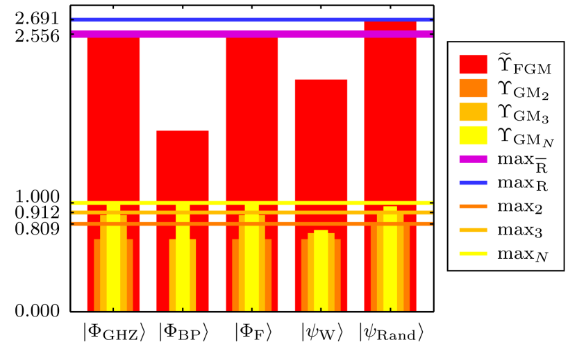
Figure 3: (color online) Unnormalized FGM ent $\widetilde{\Upsilon}_{\text{FGM}}$ of (6) for the test states of (14), with only the $|\psi_{\text{Rand}}\rangle$ that maximizes it after $1000$ random pure states were tested. The normalized $\text{GM}_{k}$ ents $\Upsilon_{\text{GM}_{k}}$ of (7) are also shown, and the maximum of each over all test states is $\max_{k}\equiv\max(\Upsilon_{\text{GM}_{k}})$, while $\max_{{\kern 0.5pt}\overline{\rule{0.0pt}{5.0pt}{\kern-0.1pt}\text{R}{\kern-0.6pt}}}\equiv$ $\max(\widetilde{\Upsilon}_{\text{FGM}})$ applies to all nonrandom test states, and $\max_{{\kern 0.5pt}\text{R}}\equiv\max(\widetilde{\Upsilon}_{\text{FGM}}(\rho_{|\psi_{\text{Rand}}\rangle}))$.

As Fig.3 shows, the maximally $\text{F}_{N}$-entangled ($N=4$) states $|\Phi_{\text{GHZ}}\rangle$ and $|\Phi_{\text{F}}\rangle$ have identical results for all $\Upsilon_{\text{GM}_{k}}$ and $\widetilde{\Upsilon}_{\text{FGM}}$, but the maximally $\text{F}_{N}$-entangled $|\Phi_{\text{BP}}\rangle$ has $\Upsilon_{\text{GM}_{2}}=0$ and therefore a lower $\widetilde{\Upsilon}_{\text{FGM}}$, despite matching $|\Phi_{\text{GHZ}}\rangle$ and $|\Phi_{\text{F}}\rangle$ for $\Upsilon_{\text{GM}_{N}}$. As expected, $|\psi_{\text{W}}\rangle$ is not maximal in any quantity, but still has fairly high values, and actually outperforms $|\Phi_{\text{BP}}\rangle$ in $\Upsilon_{\text{GM}_{2}}$, $\Upsilon_{\text{GM}_{3}}$, and $\widetilde{\Upsilon}_{\text{FGM}}$, despite its lower $\Upsilon_{\text{GM}_{N}}$.

Interestingly, $|\psi_{\text{Rand}}\rangle$ reached a higher $\widetilde{\Upsilon}_{\text{FGM}}$ than all other test states, since its $\Upsilon_{\text{GM}_{2}}$ and $\Upsilon_{\text{GM}_{3}}$ are higher than those of the other states, while its $\Upsilon_{\text{GM}_{N}}$ is still slightly lower than $1$. This proves by example that there are nonmaximally-$\text{F}_{N}$-entangled FGM-entangled states with higher $\widetilde{\Upsilon}_{\text{FGM}}$ than maximally $\text{F}_{N}$-entangled states.

III.2 Tests and Analysis of FSM Ent

Here, Fig.4 applies the same tests as in Fig.3, but this time for the FSM ent of (8).

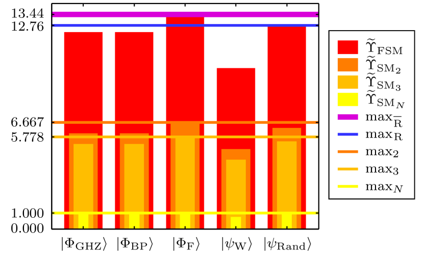
Figure 4: (color online) Unnormalized FSM ent $\widetilde{\Upsilon}_{\text{FSM}}$ of (8) for the test states of (14), with only the $|\psi_{\text{Rand}}\rangle$ that maximizes it over $1000$ random pure states. The unnormalized $\text{SM}_{k}$ ents $\widetilde{\Upsilon}_{\text{SM}_{k}}$ of (9) are also shown, and the maximum of each over all test states is $\max_{k}\equiv\max(\widetilde{\Upsilon}_{\text{SM}_{k}})$, while $\max_{{\kern 0.5pt}\overline{\rule{0.0pt}{5.0pt}{\kern-0.1pt}\text{R}{\kern-0.6pt}}}\equiv$ $\max(\widetilde{\Upsilon}_{\text{FSM}})$ applies to all nonrandom test states, and $\max_{{\kern 0.5pt}\text{R}}\equiv\max(\widetilde{\Upsilon}_{\text{FSM}}(\rho_{|\psi_{\text{Rand}}\rangle}))$.

Here, we see that $|\Phi_{\text{BP}}\rangle$ has the same $\widetilde{\Upsilon}_{\text{SM}_{k}}$ and $\widetilde{\Upsilon}_{\text{FSM}}$ as $|\Phi_{\text{GHZ}}\rangle$, but that both $|\Phi_{\text{GHZ}}\rangle$ and $|\Phi_{\text{BP}}\rangle$ underperform $|\Phi_{\text{F}}\rangle$ in terms of $\widetilde{\Upsilon}_{\text{SM}_{2}}$, $\widetilde{\Upsilon}_{\text{SM}_{3}}$, and $\widetilde{\Upsilon}_{\text{FSM}}$, despite all three states being maximally $\text{F}_{N}$-entangled. This time, $|\psi_{\text{W}}\rangle$ underperforms all other test states in every area, while $|\psi_{\text{Rand}}\rangle$ outperforms $|\Phi_{\text{GHZ}}\rangle$ and $|\Phi_{\text{BP}}\rangle$, while still underperforming $|\Phi_{\text{F}}\rangle$, suggesting that $|\Phi_{\text{F}}\rangle$ may be maximal in all quantities being measured.

Thus, this proves by example that some maximally $\text{F}_{N}$-entangled states are more FSM-entangled than others, even $|\Phi_{\text{GHZ}}\rangle$, and suggests that maximally FSM-entangled states may also be maximal for all $\Upsilon_{\text{SM}_{k}}$.

III.3 Tests and Analysis of FDM Ent

Here we apply the same tests as in Sec.III.1 and Sec.III.2, this time to the FDM ent of (10).

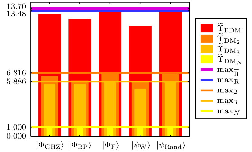
Figure 5: (color online) Unnormalized FDM ent $\widetilde{\Upsilon}_{\text{FDM}}$ (or ent-concurrence) of (10) for the test states of (14), with only the $|\psi_{\text{Rand}}\rangle$ that maximizes it over $1000$ random pure states. The unnormalized $\text{DM}_{k}$ ents $\widetilde{\Upsilon}_{\text{DM}_{k}}$ of (11) are also shown, and the maximum of each over all test states is $\max_{k}\equiv\max(\widetilde{\Upsilon}_{\text{DM}_{k}})$, while $\max_{{\kern 0.5pt}\overline{\rule{0.0pt}{5.3pt}{\kern-0.1pt}\text{R}{\kern-0.6pt}}}\equiv\max(\widetilde{\Upsilon}_{\text{FDM}})$ applies to all nonrandom test states, and $\max_{{\kern 0.5pt}\text{R}}\!\equiv\!\max(\widetilde{\Upsilon}_{\text{FDM}}(\rho_{|\psi_{\text{Rand}}\rangle}))$.

Figure 5 shows different results for $|\Phi_{\text{GHZ}}\rangle$ and $|\Phi_{\text{BP}}\rangle$, which is mainly due to the one biseparability of $|\Phi_{\text{BP}}\rangle$, making the FDM ent the only measure of these three that distinguishes between the separability of these states, and yet does not neglect the other bipartite entanglement correlations in $|\Phi_{\text{BP}}\rangle$. Again, $|\Phi_{\text{F}}\rangle$ seems to outperform all other states in every measure, as suggested by the fact that $|\psi_{\text{Rand}}\rangle$ seems to approach its performance, and $|\psi_{\text{W}}\rangle$ slightly underperforms in every area.

III.4 Comparison of FGM, FSM, and FDM Ents

The most important difference between $\Upsilon_{\text{FGM}}$ and both $\Upsilon_{\text{FSM}}$ and $\Upsilon_{\text{FDM}}$ is that ${\Upsilon}_{\text{GM}_{2}}(\rho_{|\Phi_{\text{BP}}\rangle})=0$ while $\widetilde{\Upsilon}_{\text{SM}_{2}}(\rho_{|\Phi_{\text{BP}}\rangle})\neq 0$ and $\widetilde{\Upsilon}_{\text{DM}_{2}}(\rho_{|\Phi_{\text{BP}}\rangle})\neq 0$. The fact that not all bipartitions of $|\Phi_{\text{BP}}\rangle$ are separable means that there are some bipartitions that have entanglement correlations, and the sum over all $2$-partitional quantities in $\widetilde{\Upsilon}_{\text{SM}_{2}}$ and $\widetilde{\Upsilon}_{\text{DM}_{2}}$ is why they detect these correlations, while the minimum over all $2$-partitions in ${\Upsilon}_{\text{GM}_{2}}$ is why it misses those entanglement correlations, reporting “zero.” Therefore ${\Upsilon}_{\text{GM}_{2}}$ is not sufficient to detect all entanglement correlations of $2$-partitions of a state, so $\Upsilon_{\text{FGM}}$ is not sufficient to detect all entanglement correlations.

Thus, we must make an important new distinction; presence of separability in a particular $k$-partition is not sufficient to claim absence of entanglement correlations over all $k$-partitions for a given $k$. Since nonseparable nonlocal correlations (NSNLC) are what the word entanglement really means, we must require the necessary and sufficient detection of the presence of any NSNLC as our prime criterion for what constitutes an entanglement measure. We state all of this in the following theorem.

True-Entanglement Theorem:  The absence of separability between any partitions is necessary and sufficient for the presence of any entanglement correlations, and therefore the presence of true entanglement. In other words; the presence of separability between all partitions is necessary and sufficient for the absence of all entanglement correlations, and thus the absence of true entanglement.

This theorem reflects the fact that although a state may be separable over one particular $k$-partition, that is not sufficient to conclude the absence of all $k$-partite entanglement correlations, so sub-$N$ $k$-separability is not a sufficient criterion for the absence of all $k$-partite NSNLC.

The likely reason that $\text{GM}_{k}$-entanglement was defined with the min function is that the presence of separability in any one bipartition is sufficient to claim the absence of entanglement correlations for bipartite systems, since there is only one bipartition. So if separability were our only concern for multimode systems, then $\text{GM}_{k}$-entanglement would be correctly defined because if a state is in any way $k$-separable, then its $\text{GM}_{k}$-entanglement is $0$. (After all, GM measures do correctly indicate whether a pure state is a product over at least one $k$-partition.) But since we have just seen examples that $k$-separability is not sufficient to conclude the absence of all $k$-partite NSNLC, and since NSNLC are what entanglement really is, then $\text{GM}_{k}$-“entanglement” is not really a measure of $k$-partite entanglement.

Unfortunately, there is now quite a lot of literature that uses the terminology (GM)-“$k$-entangled” to describe a condition that is insufficient to determine the presence of entanglement correlations over all $k$-partitions. Our remedy for this was to observe the fact that the absence of $k$-separability is the condition of all $k$-partitions not having $k$-mode product form, which motivated us to sum the $N$-mode $k$-partitional entanglement values over all $k$-partitions in our various candidate entanglement measures in Sec.II. These sums gave us candidate $\text{F}_{k}$-entanglement values which were further added over all $k$ values to construct candidate measures for detecting all possible entanglement correlations in a given pure state.

However, the True-Entanglement Theorem alone is not sufficient to distinguish between states like $|\Phi_{\text{GHZ}}\rangle$ and $|\Phi_{\text{BP}}\rangle$. One missing concept is that the states that are most entangled have the most simultaneous entanglement correlations over all possible partitions. Since this is exactly what the FSM ent measures, then it is both necessary and sufficient to detect all entanglement correlations, and it measures their simultaneous presence, providing an ordering for multipartite entangled states.

Yet the FSM ent’s ordering is still not sufficient to reveal the difference between states like $|\Phi_{\text{GHZ}}\rangle$ and $|\Phi_{\text{BP}}\rangle$, as seen in Fig.4. Therefore, by also requiring that the simultaneous entanglement correlations be as evenly and as widely distributed as possible, we attain ordering criteria that distinguish $|\Phi_{\text{GHZ}}\rangle$ and $|\Phi_{\text{BP}}\rangle$ without sacrificing information about entanglement correlations. The FDM ent (ent-concurrence) may achieve this, as seen in Fig.5.

However, the True-Entanglement Theorem only applies to applications of entanglement in the full Hilbert space of $\rho$. For applications of entanglement in the reductions, other principles are involved, as discussed in Sec.VII.

IV Candidate Mixed-State Measures

\begin{picture}(100.0,0.0)\put(1.0,24.0){\hypertarget{Sec:IV}{}} \end{picture}

Here we list the mixed-state entanglement-measure candidates that we test in Sec.V. In all cases, $\hat{E}(\rho)$ means the convex-roof extension of a pure-state measure $E(\rho)$ to handle mixed-state input (see (Hedemann, 2016, App.J)).

• The FGM ent of formation (using $\Upsilon_{\text{FGM}}(\rho)$ from (6)):

  $$\hat{\Upsilon}_{\text{FGM}}(\rho)\equiv\!\mathop{\min}\limits_{\{p_{j},\rho_{j}\}|_{\rho=\sum\nolimits_{j}{p_{j}\rho_{j}}}}\!\!\left({\sum\nolimits_{j}{p_{j}\Upsilon_{\text{FGM}}(\rho_{j})}}\!\right)\!.$$ (16)

• The strict FGM (SFGM) ent of formation:

  $$\Upsilon_{\text{SFGM}}(\rho)\equiv\frac{1}{M_{\text{SFGM}}}\sum\limits_{k=2}^{N}{\Upsilon_{\text{SGM}_{k}}(\rho)},$$ (17)

  where $M_{\text{SFGM}}$ is a normalization factor, and the strict $\text{GM}_{k}$ ($\text{SGM}_{k}$) ent of formation is

  $$\Upsilon_{\text{SGM}_{k}}(\rho)\equiv\min(\{\hat{\Upsilon}^{(\mathbf{N}_{h}^{(\mathbf{k})})}(\rho)\}),$$ (18)

  where $\{\hat{\Upsilon}^{(\mathbf{N}_{h}^{(\mathbf{k})})}(\rho)\}$ is the set of convex-roof extensions of all $N$-mode $k$-partitional ents. Here, the minimum over all convex-roof-extensions of a given kind of $k$-partitional ent ensures that if a state achieves strict $k$-separability, all of its optimal-decomposition pure states are $k$-separable over the same partitions.

• The FSM ent of formation (using $\Upsilon_{\text{FSM}}(\rho)$ from (8)):

  $$\hat{\Upsilon}_{\text{FSM}}(\rho)\equiv\!\mathop{\min}\limits_{\{p_{j},\rho_{j}\}|_{\rho=\sum\nolimits_{j}{p_{j}\rho_{j}}}}\!\!\left({\sum\nolimits_{j}{p_{j}\Upsilon_{\text{FSM}}(\rho_{j})}}\!\right)\!.$$ (19)

• The FDM ent of formation (with $\Upsilon_{\text{FDM}}(\rho)$ from (10)):

  $$\hat{\Upsilon}_{\text{FDM}}(\rho)\equiv\!\mathop{\min}\limits_{\{p_{j},\rho_{j}\}|_{\rho=\sum\nolimits_{j}{p_{j}\rho_{j}}}}\!\!\left({\sum\nolimits_{j}{p_{j}\Upsilon_{\text{FDM}}(\rho_{j})}}\!\right)\!.$$ (20)

We do not use a “hat” if a convex-roof extension (CRE) has been applied already within the function.

V Tests of Candidate Mixed-State Measures

\begin{picture}(100.0,0.0)\put(1.0,27.0){\hypertarget{Sec:V}{}} \end{picture}

Limiting ourselves to rank-2 mixed states (since CREs of those are practical to approximate) we use test states,

$$\begin{array}[]{*{20}l}{\rho_{\text{GHZ}+1}}&\!\!{\equiv\frac{1}{2}(|\Phi_{\text{GHZ}}\rangle\langle\Phi_{\text{GHZ}}|+|1,\!1,\!1,\!1\rangle\langle 1,\!1,\!1,\!1|)}\\ {\rho_{2\text{-sep}}}&\!\!\rule{0.0pt}{9.8pt}{\equiv\frac{1}{2}(\rho_{|\Phi^{+}\rangle\otimes|\Phi^{+}\rangle}+\rho_{|1\rangle}^{(1)}\otimes|\Phi_{\text{GHZ}_{3}}\rangle\langle\Phi_{\text{GHZ}_{3}}|)}\\ {\rho_{\text{F}+1}}&\!\!\rule{0.0pt}{9.8pt}{\equiv\frac{1}{2}(|\Phi_{\text{F}}\rangle\langle\Phi_{\text{F}}|+|1,\!1,\!1,\!1\rangle\langle 1,\!1,\!1,\!1|)}\\ {\rho_{\text{MME}}}&\!\!\rule{0.0pt}{9.8pt}{\equiv\frac{1}{2}(\rho_{{\textstyle{1\over{\sqrt{2}}}}(|1,{\kern-0.5pt}1,{\kern-0.5pt}1,{\kern-0.5pt}1\rangle+|2,{\kern-0.5pt}2,{\kern-0.5pt}2,{\kern-0.5pt}1\rangle)}\!+\!\rho_{{\textstyle{1\over{\sqrt{2}}}}(|1,{\kern-0.5pt}1,{\kern-0.5pt}1,{\kern-0.5pt}2\rangle+|2,{\kern-0.5pt}2,{\kern-0.5pt}2,{\kern-0.5pt}2\rangle)})}\\ {\rho_{|\Phi_{\text{F}}\rangle}}&\!\!\rule{0.0pt}{9.8pt}{\equiv|\Phi_{\text{F}}\rangle\langle\Phi_{\text{F}}|,}\\ \end{array}$$ (21)

where $\rho_{\textnormal{\raisebox{0.5pt}[0.5pt][0.5pt]{$|A\rangle$}}}\!\equiv\!|A\rangle\langle A|$, and $|\Phi_{\text{GHZ}}\rangle$, $|\Phi^{+}\rangle\otimes|\Phi^{+}\rangle\!\equiv\!|\Phi_{\text{BP}}\rangle$, and $|\Phi_{\text{F}}\rangle$ are from (14), $\rho_{\textnormal{\raisebox{0.5pt}[0.5pt][0.5pt]{$\textnormal{\scalebox{0.9}{$|1\rangle$}}$}}}^{{\kern 0.5pt}\textnormal{\raisebox{0.5pt}[0.5pt][0.5pt]{$\textnormal{\scalebox{0.9}{$(1)$}}$}}}$ is the first computational basis state for the mode-$1$ qubit, and $|\Phi_{\text{GHZ}_{3}}\rangle\equiv$ ${\textstyle{1\over{\sqrt{2}}}}(|1,\!1,\!1\rangle\langle 1,\!1,\!1|\!+\!|2,\!2,\!2\rangle\langle 2,\!2,\!2|)$ is a $3$-qubit GHZ state.

We include $\rho_{\text{GHZ}+1}$ and $\rho_{\text{F}+1}$ because they are mixtures of highly entanglement-correlated states with a basis state they already include, to see how the candidate measures rate this lowering of entanglement correlation.

To test a state like (2), $\rho_{2\text{-sep}}$ decomposes into pure states that are each $2$-separable in different ways, where each part has strong internal entanglement correlations.

The state $\rho_{\text{MME}}$, when viewed as a $2\times 8$ system is a mixed state with the same entanglement as a maximally entangled pure state. Rediscovered in the present work, this phenomenon was originally discovered in Cavalcanti et al. (2005); Li et al. (2012), and called “mixed maximally entangled (MME) states.” It is easy to prove that all decompositions of such states consist of maximally entangled pure decomposition states, yielding an entanglement of $1$ by any unit-normalized convex-roof (or nearest-separable-state Streltsov et al. (2010)) measure.

We use pure state $\rho_{|\Phi_{\text{F}}\rangle}$ as a reference since it had near-highest values in the GM measures of Fig.3, and it may have the highest values for the SM measures in Fig.4 and the DM measures in Fig.5.

V.1 Tests and Analysis of Mixed-Input FGM Ents

Figures 6–7 show similar results but differ in subtle ways briefly explained after each.

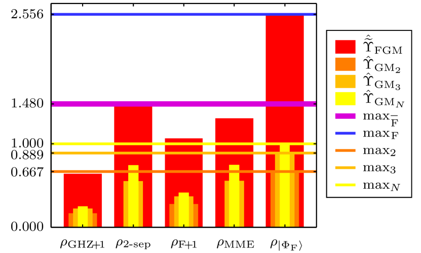
Figure 6: (color online) Unnormalized FGM ent of formation $\textnormal{\scalebox{0.8}{$\hat{\widetilde{\Upsilon}}$}}_{\text{FGM}}$ of (16) approximated for the test states of (21). The (normalized) $\text{GM}_{k}$ ents of formation ${\hat{\Upsilon}}_{\text{GM}_{k}}$ (CREs of (7)) are also approximated, and the maximum of each over all test states is $\max_{k}\equiv\max(\hat{\Upsilon}_{\text{GM}_{k}})$, while $\max_{{\kern 0.5pt}\overline{\rule{0.0pt}{5.3pt}{\kern-0.1pt}\text{F}{\kern-0.6pt}}}\equiv$ $\max(\textnormal{\scalebox{0.8}{$\hat{\widetilde{\Upsilon}}$}}_{\text{FGM}})$ applies to all non$\rho_{|\Phi_{\text{F}}\rangle}$ test states, and $\max_{{\kern 0.5pt}\text{F}}\equiv\max(\textnormal{\scalebox{0.8}{$\hat{\widetilde{\Upsilon}}$}}_{\text{FGM}}(\rho_{|\Phi_{\text{F}}\rangle}))$. The CRE approximations used $900$ decompositions, as in Hedemann (2016).

The main items of interest in Fig.6 are the fact that both $\rho_{2\text{-sep}}$ and $\rho_{\text{MME}}$ have ${\hat{\Upsilon}}_{\text{GM}_{2}}=0$, and while we expect this to be true from the way the FGM ent minimizes over all bipartitions for each decomposition state within the larger minimization of the CRE, it shows that GM measures ignore entanglement correlations, since $\rho_{\text{MME}}$ in particular has the maximal entanglement of a pure state for the $(1|2,3,4)$ bipartition, as mentioned earlier.

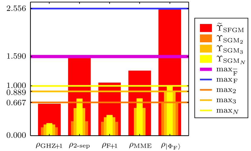
Figure 7: (color online) Unnormalized SFGM ent of formation ${\widetilde{\Upsilon}}_{\text{SFGM}}$ of (17) approximated for the test states of (21). The (normalized) $\text{SGM}_{k}$ ents of formation ${{\Upsilon}}_{\text{SGM}_{k}}$ of (18) are also approximated, and the maximum of each over all test states is $\max_{k}\equiv\max({\Upsilon}_{\text{SGM}_{k}})$, while $\max_{{\kern 0.5pt}\overline{\rule{0.0pt}{5.3pt}{\kern-0.1pt}\text{F}{\kern-0.6pt}}}\equiv$ $\max({\widetilde{\Upsilon}}_{\text{SFGM}})$ applies to all non$\rho_{|\Phi_{\text{F}}\rangle}$ test states, and $\max_{{\kern 0.5pt}\text{F}}\equiv\max({\widetilde{\Upsilon}}_{\text{SFGM}}(\rho_{|\Phi_{\text{F}}\rangle}))$. CRE approximations used $900$ decompositions.

The strict version, the SFGM ent of formation ${\widetilde{\Upsilon}}_{\text{SFGM}}$ in Fig.7 does slightly better than $\textnormal{\scalebox{0.8}{$\hat{\widetilde{\Upsilon}}$}}_{\text{FGM}}$ in Fig.6 because it correctly detects that no bipartitions of $\rho_{2\text{-sep}}$ are without entanglement correlation since its ${\Upsilon}_{\text{SGM}_{2}}\neq 0$, but it still completely ignores the maximal bipartite entanglement correlation in $\rho_{\text{MME}}$, for which ${\Upsilon}_{\text{SGM}_{2}}=0$.

We discuss further issues with GM measures regarding states like $\rho_{2\text{-sep}}$ and (2) in App.H.

V.2 Tests and Analysis of Mixed-Input FSM Ent

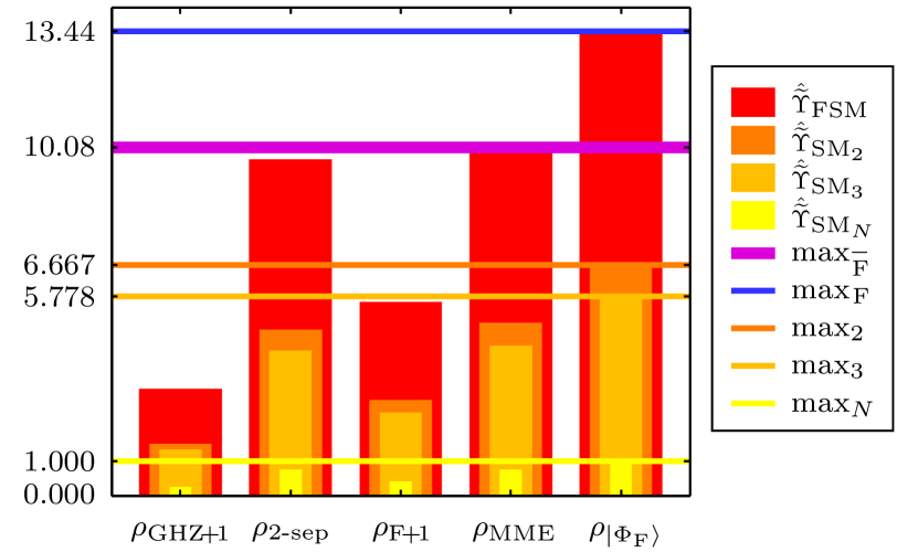
Figure 8: (color online) Unnormalized FSM ent of formation

$\hat{\widetilde{\Upsilon}}$

${}_{\text{FSM}}$ of (19) approximated for the test states of (21). The unnormalized $\text{SM}_{k}$ ents of formation

${\hat{\widetilde{\Upsilon}}}$

${}_{\text{SM}_{k}}$ (CREs of (9)) are also approximated, and the maximum of each over all test states is $\max_{k}\equiv\max($

$\hat{\widetilde{\Upsilon}}$

${}_{\text{SM}_{k}})$, while $\max_{{\kern 0.5pt}\overline{\rule{0.0pt}{5.3pt}{\kern-0.1pt}\text{F}{\kern-0.6pt}}}\,\equiv\,$ $\max($

$\hat{\widetilde{\Upsilon}}$

${}_{\text{FSM}})$ applies to all non$\rho_{\textnormal{\raisebox{0.5pt}[0.5pt][0.5pt]{$|\Phi_{\text{F}}\rangle$}}}$ test states, and $\max_{{\kern 0.5pt}\text{F}}\!\equiv\!\max($

$\hat{\widetilde{\Upsilon}}$

${}_{\text{FSM}}(\rho_{|\Phi_{\text{F}}\rangle}))$. CRE approximations used $900$ decompositions.

Figure 8 tests unnormalized FSM ent of formation from (19), and we see that the known bipartite entanglement correlations in both $\rho_{2\text{-sep}}$ and $\rho_{\text{MME}}$ are detected since ${\hat{\widetilde{\Upsilon}}}$ ${}_{\text{SM}_{2}}\neq 0$ for each.

V.3 Tests and Analysis of Mixed-Input FDM Ent (The Ent-Concurrence)

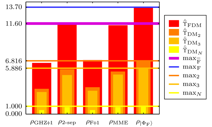
Figure 9: (color online) Unnormalized FDM ent of formation (ent-concurrence of formation)

$\hat{\widetilde{\Upsilon}}$

${}_{\text{FDM}}$ of (20) approximated for the test states of (21). The unnormalized $\text{DM}_{k}$ ents of formation

${\hat{\widetilde{\Upsilon}}}$

${}_{\text{DM}_{k}}$ (CREs of (11)) are also approximated, and the maximum of each over all test states is $\max_{k}\equiv\max($

$\hat{\widetilde{\Upsilon}}$

${}_{\text{DM}_{k}})$, while $\max_{{\kern 0.5pt}\overline{\rule{0.0pt}{5.3pt}{\kern-0.1pt}\text{F}{\kern-0.6pt}}}\equiv$ $\max($

$\hat{\widetilde{\Upsilon}}$

${}_{\text{FDM}})$ applies to all non$\rho_{\textnormal{\raisebox{0.5pt}[0.5pt][0.5pt]{$|\Phi_{\text{F}}\rangle$}}}$ test states, and $\max_{{\kern 0.5pt}\text{F}}\equiv\max($

$\hat{\widetilde{\Upsilon}}$

${}_{\text{FDM}}(\rho_{|\Phi_{\text{F}}\rangle}))$. CRE approximations used $900$ decompositions.

Here in Fig.9, we see the ratings of $\hat{\widetilde{\Upsilon}}$ ${}_{\text{FDM}}$ are similar to those of $\hat{\widetilde{\Upsilon}}$ ${}_{\text{FSM}}$ in Fig.8, except that here, the values for $\rho_{\text{GHZ}+1}$ are much closer to the values for $\rho_{\text{F}+1}$ (though still less than they are). Thus, this test does not show any apparent problems, and exhibits the necessary features that neither $\rho_{2\text{-sep}}$ nor $\rho_{\text{MME}}$ can be considered free of $2$-partite entanglement correlations (see App.H).

V.4 Comparison of all Mixed-Input Candidates

The main difference between the GM measures (from (16) and (17)) and the SM and DM measures of (19) and (20) is that the GM measures tend to undervalue the amount of entanglement, which is a consequence of their interpretation of separability as the prime criterion for lack of entanglement. The SM and DM measures take a more global approach, checking every possible $k$-partition for the presence of entanglement correlations, and as such, they correctly detect entanglement of every $k$-partitional type, in particular correctly not ignoring the maximal bipartite entanglement in $\rho_{\text{MME}}$.

In the pure-input case, the FDM ent $\Upsilon_{\text{FDM}}$ was the only measure that could distinguish between $|\Phi_{\text{GHZ}}\rangle$ and $|\Phi_{\text{BP}}\rangle$ without sacrificing detection of entanglement correlations, and it equals the concurrence $C$ for two qubits. Since $C$ for mixed states is a convex-roof extension (CRE), and since $\hat{\Upsilon}_{\text{FDM}}$ is also a CRE, then $\hat{\Upsilon}_{\text{FDM}}=C$ for mixed two-qubit states, as well.

VI Ent-Concurrence

\begin{picture}(100.0,0.0)\put(1.0,24.0){\hypertarget{Sec:VI}{}} \end{picture}

The ability of $\hat{\Upsilon}_{\text{FDM}}$ to detect and distinguish multipartite entanglement correlations and its link to $C$ both suggest that we adopt it as a universal measure of multipartite entanglement, called the ent-concurrence,

$$\hat{C}_{\Upsilon}(\rho)\equiv\hat{\Upsilon}_{\text{FDM}}(\rho),$$ (22)

where $\hat{\Upsilon}_{\text{FDM}}$ is defined in (20), so that

$$\begin{array}[]{*{20}l}{\hat{C}_{\Upsilon}(\rho)}&\!\!{\kern-0.5pt}{\equiv\!\!{\kern 0.5pt}\mathop{\min}\limits_{\{p_{j},\rho_{j}\}|_{\rho=\sum\nolimits_{j}{p_{j}\rho_{j}}}}\!\!\!{\kern 0.5pt}\left(\!{\kern 0.5pt}{\sum\limits_{j}{\kern-0.5pt}{p_{j}\!{\kern-0.5pt}\sum\limits_{k=2}^{N}\frac{1}{M_{k}}\sum\limits_{h=1}^{\{_{\,k}^{N}\}}\!\!\sqrt{{\kern-1.0pt}\Upsilon^{(\mathbf{N}_{h}^{(\mathbf{k})})}(\rho_{j}){\kern-1.0pt}}}}{\kern 1.0pt}\right)\!{\kern-1.0pt},}\\ \end{array}\!$$ (23)

where $M_{k}\equiv M_{\text{FDM}}M_{\text{DM}_{k}}$ is a normalization factor based on those of (10) and (11), and $\{_{{\kern 1.0pt}k}^{N}\}$ are Stirling numbers of the second kind as in (9), which is the number of different $N$-mode $k$-partitional ents $\Upsilon^{\textnormal{\raisebox{-0.8pt}[-0.8pt][-0.8pt]{$(\mathbf{N}_{{\kern-0.5pt}\textnormal{\raisebox{-0.5pt}[-0.5pt][-0.5pt]{$h$}}}^{{\kern 0.5pt}\textnormal{\raisebox{-0.3pt}[-0.3pt][-0.3pt]{$(\mathbf{k})$}}})$}}}(\rho)$.

While $\hat{C}_{\Upsilon}$ detects all entanglement and distinguishes between different types of $\text{F}_{k}$-entanglement, it may also be useful to have a partition-specific view of how much entanglement exists between particular mode groups. Therefore, in the notation of Hedemann (2016), we also define the $N$-mode partitional ent-concurrence vector as

$$\Xi_{C_{\Upsilon}}^{(\mathbf{N})}(\rho)\equiv\!\left({\begin{array}[]{*{20}c}{\{\hat{C}_{\Upsilon}^{(\mathbf{N}_{h}^{(\mathbf{2})})}(\rho)\}}\\ \vdots\\ {\{\hat{C}_{\Upsilon}^{(\mathbf{N}_{h}^{(\mathbf{N})})}(\rho)\}}\\ \end{array}}\right)\!,$$ (24)

where $\{\hat{C}_{\Upsilon}^{(\mathbf{N}_{h}^{(\mathbf{k})})}(\rho)\}$ is the set of all $N$-mode $k$-partitional ent-concurrences of formation, the pure-input versions of which are in (13). For example, in a $4$-mode system,

where, for instance,

$$\hat{C}_{\Upsilon}^{(2|1,3,4)}=\!\mathop{\min}\limits_{\{p_{j},\rho_{j}\}|_{\rho=\sum\nolimits_{j}{p_{j}\rho_{j}}}}\!\!\left({\sum\nolimits_{j}{p_{j}\sqrt{\Upsilon^{(2|1,3,4)}(\rho_{j})}}}\,\right)\!.$$ (26)

Thus, the top row of $\Xi_{\textnormal{\raisebox{0.5pt}[0.5pt][0.5pt]{${\kern 0.5pt}C_{\Upsilon}$}}}^{\textnormal{\raisebox{2.5pt}[2.5pt][2.5pt]{$(\mathbf{N})$}}}$ lists all contributions to $\text{F}_{2}$-entanglement, and so-on until the lowest row gives the $\text{F}_{N}$-entanglement, yielding a fine-grained view of the entanglement between each possible mode group.

For an intermediate view of entanglement, we can define the $N$-mode $k$-ent-concurrences of formation as

$$\hat{C}_{\Upsilon_{k}}(\rho)\equiv\hat{\Upsilon}_{\text{DM}_{k}}(\rho),$$ (27)

which is a CRE of a $1$-norm over all $C_{\Upsilon}^{(\mathbf{N}_{h}^{(\mathbf{k})})}(\rho)$ for a given $k$, as seen from (13) and the definition of $\Upsilon_{\text{DM}_{k}}(\rho)$ in (11).

Hierarchy of Maximally $\text{F}_{N}$-Entangled TGX States

The ent-concurrence identifies a hierarchy among the maximally $\text{F}_{N}$-entangled states, which is easiest to see by examining its values for the subset of $\text{F}_{N}$-entangled TGX states from App.G, as in Table 1.

Table 1: Normalized ent-concurrence $C_{\Upsilon}$ and normalized $k$-ent-concurrences $C_{\Upsilon_{k}}$ for each of the maximally $\text{F}_{N}$-entangled $4$-qubit TGX states $|\Phi_{{j}}^{[L_{*}]}\rangle$ involving the first computational basis state $|1\rangle\equiv|1,\!1,\!1,\!1\rangle$, from App.G, where $L_{*}$ is the number of levels with nonzero state coefficients. Normalizations are over these states alone, and may not be the normalizations over all states. The test states of (14) are $|\Phi_{\text{GHZ}}\rangle\equiv|\Phi_{1}^{[2]}\rangle$, $|\Phi_{\text{BP}}\rangle\equiv|\Phi_{1}^{[4]}\rangle$, and $|\Phi_{\text{F}}\rangle\equiv|\Phi_{2}^{[4]}\rangle$, in the first three rows.

$|\Phi_{j}^{[L_{*}]}\rangle$	$C_{\Upsilon}$	$C_{\Upsilon_{2}}$	$C_{\Upsilon_{3}}$	$C_{\Upsilon_{N}}$
$|\Phi_{1}^{[2]}\rangle$	$0.957$	$0.946$	$0.961$	$1.000$
$|\Phi_{1}^{[4]}\rangle$	$0.922$	$0.880$	$0.957$	$1.000$
$|\Phi_{2}^{[4]}\rangle$	$1.000$	$1.000$	$1.000$	$1.000$
$|\Phi_{3}^{[4]}\rangle$	$0.922$	$0.880$	$0.957$	$1.000$
$|\Phi_{4}^{[4]}\rangle$	$1.000$	$1.000$	$1.000$	$1.000$
$|\Phi_{5}^{[4]}\rangle$	$0.922$	$0.880$	$0.957$	$1.000$
$|\Phi_{6}^{[4]}\rangle$	$1.000$	$1.000$	$1.000$	$1.000$
$|\Phi_{7}^{[4]}\rangle$	$1.000$	$1.000$	$1.000$	$1.000$
$|\Phi_{8}^{[4]}\rangle$	$1.000$	$1.000$	$1.000$	$1.000$
$|\Phi_{9}^{[4]}\rangle$	$1.000$	$1.000$	$1.000$	$1.000$
$|\Phi_{1}^{[6]}\rangle$	$0.957$	$0.946$	$0.961$	$1.000$
$|\Phi_{2}^{[6]}\rangle$	$0.957$	$0.946$	$0.961$	$1.000$
$|\Phi_{3}^{[6]}\rangle$	$0.957$	$0.946$	$0.961$	$1.000$
$|\Phi_{1}^{[8]}\rangle$	$0.957$	$0.946$	$0.961$	$1.000$

In Table 1, the highest-rated maximally $\text{F}_{N}$-entangled TGX states, having $(C_{\Upsilon},\!C_{\Upsilon_{2}},\!C_{\Upsilon_{3}},\!C_{\Upsilon_{N}})=(1,\!1,\!1,\!1)$, are the tier-1 $\text{F}_{N}$-entangled states,

$$\begin{array}[]{*{20}l}{|\Phi_{2}^{[4]}\rangle}&\!\!\!{=\!{\textstyle{1\over{\sqrt{4}}}}(|1111\rangle\!+\!|1122\rangle\!+\!|2212\rangle\!+\!|2221\rangle)}\\ {|\Phi_{4}^{[4]}\rangle}&\!\!\!{=\!{\textstyle{1\over{\sqrt{4}}}}(|1111\rangle\!+\!|1212\rangle\!+\!|2122\rangle\!+\!|2221\rangle)}\\ {|\Phi_{6}^{[4]}\rangle}&\!\!\!{=\!{\textstyle{1\over{\sqrt{4}}}}(|1111\rangle\!+\!|1221\rangle\!+\!|2122\rangle\!+\!|2212\rangle)}\\ {|\Phi_{7}^{[4]}\rangle}&\!\!\!{=\!{\textstyle{1\over{\sqrt{4}}}}(|1111\rangle\!+\!|1222\rangle\!+\!|2112\rangle\!+\!|2221\rangle)}\\ {|\Phi_{8}^{[4]}\rangle}&\!\!\!{=\!{\textstyle{1\over{\sqrt{4}}}}(|1111\rangle\!+\!|1222\rangle\!+\!|2121\rangle\!+\!|2212\rangle)}\\ {|\Phi_{9}^{[4]}\rangle}&\!\!\!{=\!{\textstyle{1\over{\sqrt{4}}}}(|1111\rangle\!+\!|1222\rangle\!+\!|2122\rangle\!+\!|2211\rangle),}\\ \end{array}$$ (28)

where $|abcd\rangle\equiv|a,\!b,\!c,\!d\rangle$. The tier-2 $\text{F}_{N}$-entangled states, with $(C_{\Upsilon},\!C_{\Upsilon_{2}},\!C_{\Upsilon_{3}},\!C_{\Upsilon_{N}})\approx(0.957,0.946,0.961,1)$, are

and the lowest-rated group, the tier-3 $\text{F}_{N}$-entangled states, with $(C_{\Upsilon},\!C_{\Upsilon_{2}},\!C_{\Upsilon_{3}},\!C_{\Upsilon_{N}})\approx(0.922,0.880,0.957,1)$, are

$$\begin{array}[]{*{20}l}{|\Phi_{1}^{[4]}\rangle}&\!\!\!{=\!{\textstyle{1\over{\sqrt{4}}}}(|1111\rangle\!+\!|1122\rangle\!+\!|2211\rangle\!+\!|2222\rangle)}\\ {|\Phi_{3}^{[4]}\rangle}&\!\!\!{=\!{\textstyle{1\over{\sqrt{4}}}}(|1111\rangle\!+\!|1212\rangle\!+\!|2121\rangle\!+\!|2222\rangle)}\\ {|\Phi_{5}^{[4]}\rangle}&\!\!\!{=\!{\textstyle{1\over{\sqrt{4}}}}(|1111\rangle\!+\!|1221\rangle\!+\!|2112\rangle\!+\!|2222\rangle).}\\ \end{array}$$ (30)

All of these states are maximally $\text{F}_{N}$-entangled, as seen in Table 1, and furthermore, these are only a small portion of the “phaseless” maximally $\text{F}_{N}$-entangled TGX states, since similar sets can be generated by specifying a different common “starting level” than $|1\rangle=|1111\rangle$.

Whether or not other states exist that have higher ent-concurrence than the tier-1 states is still unknown, but none were found in the present numerical tests.

To see the most fine-grained view, from (25) the $N$-mode ent-concurrence vectors of $|\Phi_{\text{F}}\rangle\equiv|\Phi_{{\kern-0.5pt}2}^{{\kern 0.5pt}\textnormal{\raisebox{0.5pt}[0.5pt][0.5pt]{$\textnormal{\scalebox{0.9}{$[4]$}}$}}}\rangle$ (tier 1), $|\Phi_{\text{GHZ}}\rangle\equiv|\Phi_{{\kern-1.0pt}\textnormal{\raisebox{-0.5pt}[-0.5pt][-0.5pt]{$1$}}}^{{\kern 0.5pt}\textnormal{\raisebox{0.0pt}[0.0pt][0.0pt]{$\textnormal{\scalebox{0.9}{$[2]$}}$}}}\rangle$ (tier 2), and $|\Phi_{\text{BP}}\rangle\equiv|\Phi_{{\kern-1.0pt}\textnormal{\raisebox{-0.5pt}[-0.5pt][-0.5pt]{$1$}}}^{{\kern 0.5pt}\textnormal{\raisebox{0.0pt}[0.0pt][0.0pt]{$\textnormal{\scalebox{0.9}{$[4]$}}$}}}\rangle$ (tier 3) are

$$\Xi_{C_{\Upsilon}}^{(\mathbf{N})}(\rho_{|\Phi_{\text{F}}\rangle})=\!\left(\!\!{\begin{array}[]{*{20}c}{\begin{array}[]{*{20}c}1&1&1&1&{\sqrt{{\textstyle{2\over 3}}}}&1&1\\ \end{array}}\\ {\begin{array}[]{*{20}c}{\sqrt{{\textstyle{8\over 9}}}}&1&1&1&1&{\sqrt{{\textstyle{8\over 9}}}}\\ \end{array}}\\ 1\\ \end{array}}\!\!\right)\!,$$ (31)

$$\Xi_{C_{\Upsilon}}^{(\mathbf{N})}(\rho_{|\Phi_{\text{GHZ}}\rangle})=\!\left(\!\!{\begin{array}[]{*{20}c}{\begin{array}[]{*{20}c}1&1&1&1&{\sqrt{{\textstyle{2\over 3}}}}&{\sqrt{{\textstyle{2\over 3}}}}&{\sqrt{{\textstyle{2\over 3}}}}\\ \end{array}}\\ {\rule{0.0pt}{13.0pt}{\kern 0.1pt}\begin{array}[]{*{20}c}{\sqrt{{\textstyle{8\over 9}}}}&{\sqrt{{\textstyle{8\over 9}}}}&{\sqrt{{\textstyle{8\over 9}}}}&{\sqrt{{\textstyle{8\over 9}}}}&{\sqrt{{\textstyle{8\over 9}}}}&{\sqrt{{\textstyle{8\over 9}}}}\\ \end{array}}\\ 1\\ \end{array}}\!\!\right)\!,$$ (32)

$$\Xi_{C_{\Upsilon}}^{(\mathbf{N})}(\rho_{|\Phi_{\text{BP}}\rangle})=\!\left(\!\!{\begin{array}[]{*{20}c}{\begin{array}[]{*{20}c}1&1&1&1&0&1&1\\ \end{array}}\\ {\begin{array}[]{*{20}c}{\sqrt{{\textstyle{2\over 3}}}}&1&1&1&1&{\sqrt{{\textstyle{2\over 3}}}}\\ \end{array}}\\ 1\\ \end{array}}\!\!\right)\!.$$ (33)

The sum of all elements in each of (31–33) is the unnormalized ent-concurrence, yielding $13.70$, $13.11$, and $12.63$, respectively, which are the first three $\widetilde{\Upsilon}_{\text{FDM}}$ values (in a different order) in Fig.5. In contrast, the square of all the elements in (31–33) (since these are pure states), yields the $N$-mode ent vectors of Hedemann (2016), the sums of which yield $13.44$, $12.33$, and $12.33$, respectively, which explains why the values of $\widetilde{\Upsilon}_{\text{FSM}}$ for $|\Phi_{\text{GHZ}}\rangle$ and $|\Phi_{\text{BP}}\rangle$ are equal in Fig.4, showing that the FSM measures were not able to able to distinguish these two states.

The worth of $\Xi_{\textnormal{\scalebox{0.9}{$C_{\Upsilon}$}}}^{\textnormal{\scalebox{0.9}{$(\mathbf{N})$}}}$ is that it shows us between which mode groups entanglement and separability occur. For example, the $0$ in (33) shows that the mode groups defined by the partitioning $(1,2|3,4)$ are separable in $\rho_{\textnormal{\raisebox{0.6pt}[0.6pt][0.6pt]{$|\Phi_{\text{BP}}\rangle$}}}$, which is true since that is the Bell product, but (33) also shows that the entanglement is maximal between all other bipartitions of the state (seen in its top row). Thus, the ent-concurrence does not ignore all of these bipartite entanglement correlations just because one of them is zero, as the GM measures do.

VII Absolute Ent-Concurrence

\begin{picture}(100.0,0.0)\put(1.0,24.0){\hypertarget{Sec:VII}{}} \end{picture}

While the ent-concurrence (and its accompanying notions of $N$-mode partitional ent-concurrence vector and $k$-ent-concurrence) evaluates the multipartite entanglement resources of the entire input state in its full space, another dimension of details can be gleaned by evaluating the entanglement within reductions of the input state.

Thus for mode group $\mathbf{m}$, the $S$-mode partitional ent-concurrence vector is

$$\Xi_{C_{\Upsilon}}^{(\mathbf{m})}(\rho)\equiv\!\left({\begin{array}[]{*{20}c}{\{\hat{C}_{\Upsilon}^{(\mathbf{m}_{h}^{(\mathbf{2})})}(\rho)\}}\\ \vdots\\ {\{\hat{C}_{\Upsilon}^{(\mathbf{m}_{h}^{(\mathbf{S})})}(\rho)\}}\\ \end{array}}\right)\!,$$ (34)

where $\mathbf{m}\equiv(m_{1},\ldots,m_{S});\,S\in 2,\ldots,N$ are the modes to which $\rho\equiv\rho^{(1,\ldots,N)}$ is being reduced before being partitioned, and $\{\hat{C}_{{\kern-1.0pt}\textnormal{\raisebox{-0.9pt}[-0.9pt][-0.9pt]{${\kern 1.0pt}\textnormal{\scalebox{0.85}{$\Upsilon$}}$}}}^{{\kern 0.0pt}\textnormal{\raisebox{-0.1pt}[-0.1pt][-0.1pt]{$(\mathbf{m}_{{\kern-0.1pt}\textnormal{\raisebox{-0.6pt}[-0.6pt][-0.6pt]{$h$}}}^{{\kern 0.5pt}\textnormal{\raisebox{-0.3pt}[-0.3pt][-0.3pt]{$(\mathbf{T})$}}})$}}}\}$ is the set of all $S$-mode $T$-partitional ent-concurrences of a given reduction ${\rho}{\kern-5.3pt}{{\textnormal{\raisebox{-1.2pt}{\scalebox{1.2}{\textasciicaron}}}}}{\kern-4.2pt}{~{}}^{(\mathbf{m})}$ where $T\in 2,\ldots,S$, where for a particular partitioning labeled by $h$, the partitional ent-concurrence is

$$\hat{C}_{\Upsilon}^{(\mathbf{m}_{h}^{(\mathbf{T})})}(\rho)\!{\kern 0.5pt}\equiv\!\mathop{\min}\limits_{\{p_{j},\rho_{j}\}|_{\rho=\sum\nolimits_{j}\!{p_{j}\rho_{j}}}}\!\!\left({\sum\nolimits_{j}{p_{j}\sqrt{\Upsilon^{(\mathbf{m}_{h}^{(\mathbf{T})})}(\rho_{j})}}}\,\right)\!,$$ (35)

where $\Upsilon^{(\mathbf{m}_{h}^{(\mathbf{T})})}$ is the partitional ent (of $h$-labeled partition $\mathbf{m}_{h}^{{\kern 1.5pt}\textnormal{\raisebox{0.0pt}[0.0pt][0.0pt]{$(\mathbf{T})$}}}$) mentioned after (5) and defined in detail in Hedemann (2016). Thus, row $T{\kern-1.5pt}-{\kern-1.0pt}1$ of $\Xi_{C_{\Upsilon}}^{\textnormal{\raisebox{0.6pt}[0.6pt][0.6pt]{$(\mathbf{m})$}}}$ lists all possible $T$-partitional ent-concurrences of the mode-$\mathbf{m}$ reduction of $\rho$.

Since a partitional ent-concurrence vector exists for each reduction $\mathbf{m}$, we can define the ent-concurrence array as the matrix $\widetilde{\nabla}_{C_{\Upsilon}}$ (not a gradient) whose elements are partitional ent-concurrence vectors,

$${(\widetilde{\nabla}_{C_{\Upsilon}})}_{k,l}(\rho)\equiv\Xi_{C_{\Upsilon}}^{((\text{nCk}(\mathbf{c},k))_{l,\cdots})},$$ (36)

where $\mathbf{c}\equiv(1,\ldots,N)$, $k\in 2,\ldots,N$, and $l\in 1,\ldots,\binom{N}{k}$ where $\binom{N}{k}{\kern 0.5pt}\equiv{\kern 0.5pt}\textnormal{\raisebox{0.5pt}[0.5pt][0.5pt]{$\textnormal{\scalebox{0.92}{$\frac{N!}{k!(N-k)!}$}}$}}$, and $\text{nCk}(\mathbf{v},k)$ is the vectorized $n$-choose-$k$ function yielding the matrix whose rows are each unique combinations of the elements of $\mathbf{v}$ chosen $k$ at a time, and $A_{l,\cdots}$ is the $l$th row of matrix $A$. For example in $N=4$, (suppressing input arguments $\rho$)

$$\widetilde{\nabla}_{C_{\Upsilon}}(\rho)=\!\left(\!\!{\begin{array}[]{*{20}c}{\begin{array}[]{*{20}c}{\Xi_{C_{\Upsilon}}^{(1,2)}}&{\Xi_{C_{\Upsilon}}^{(1,3)}}&{\Xi_{C_{\Upsilon}}^{(1,4)}}&{\Xi_{C_{\Upsilon}}^{(2,3)}}&{\Xi_{C_{\Upsilon}}^{(2,4)}}&{\Xi_{C_{\Upsilon}}^{(3,4)}}\\ \end{array}}\\ {\begin{array}[]{*{20}c}{\rule{0.0pt}{12.0pt}\!\Xi_{C_{\Upsilon}}^{(1,2,3)}}&{\Xi_{C_{\Upsilon}}^{(1,2,4)}}&{\Xi_{C_{\Upsilon}}^{(1,3,4)}}&{\Xi_{C_{\Upsilon}}^{(2,3,4)}}\\ \end{array}}\\ {\rule{0.0pt}{12.0pt}\!\Xi_{C_{\Upsilon}}^{(1,2,3,4)}}\\ \end{array}}\!\!\!\right)\!,$$ (37)

where the $2$-mode partitional ent-concurrence vectors have just one element, such as

$$\Xi_{C_{\Upsilon}}^{(2,3)}=\hat{C}_{\Upsilon}^{(2|3)}=\hat{C}_{\Upsilon}^{(2,3)},$$ (38)

and $3$-mode partitional ent-concurrence vectors look like

$$\Xi_{C_{\Upsilon}}^{(1,2,4)}\!=\!\left(\!\!{\begin{array}[]{*{20}c}{\begin{array}[]{*{20}c}{\hat{C}_{\Upsilon}^{(1|2,4)}}&{\hat{C}_{\Upsilon}^{(2|1,4)}}&{\hat{C}_{\Upsilon}^{(4|1,2)}}\\ \end{array}}\\ {\hat{C}_{\Upsilon}^{(1|2|4)}}\\ \end{array}}\!\!\right)\!,$$ (39)

and the $4$-mode partitional ent-concurrence vector $\Xi_{C_{\Upsilon}}^{(1,2,3,4)}$ is given by (25).

Then, to create a universal multipartite entanglement measure that can detect all possible entanglement correlations of a state including those of all of its reductions, we can define the absolute ent-concurrence as

$$C_{\Upsilon_{\text{abs}}}(\rho)\equiv\frac{{||\widetilde{\nabla}_{C_{\Upsilon}}(\rho)||_{1}}}{{\max(||\widetilde{\nabla}_{C_{\Upsilon}}(\rho)||_{1})}}\,,$$ (40)

which is the $1$-norm over all partitional ent-concurrences normalized to its maximum value over all input states.

Thus, by Theorem 1 from App.D, $C_{\Upsilon_{\text{abs}}}$ captures a measurement of all possible ways in which a state can be entanglement-correlated. The main drawback of the absolute ent-concurrence of (40) is that it generally requires convex-roof extensions (CREs) in all elements of $\widetilde{\nabla}_{{\kern-1.5pt}C_{\Upsilon}}$, even when the input is pure, since reductions of the pure decomposition states $\rho_{j}$ of $\rho$ are generally mixed. This means that it is usually computationally intractable to calculate $C_{\Upsilon_{\text{abs}}}$, even for pure $\rho$.

For states like $|\psi_{\text{W}}\rangle$, where one of its prime characteristics is that it retains entanglement after the removal of a particle (tracing away a mode) Dür et al. (2000), finding the entanglement of its reductions is possible with the absolute ent-concurrence, and the ent-concurrence array of (36) is an excellent tool for a high-resolution picture of all possible entanglement correlations of the state. These measures would certainly show exactly how $|\psi_{\text{W}}\rangle$ differs from $|\Phi_{\text{GHZ}}\rangle$, which is separable after removal of any particles. For example, the ent-concurrence array of $|\psi_{\text{W}}\rangle$ is

$$\begin{array}[]{l}\widetilde{\nabla}_{C_{\Upsilon}}(\rho_{|\psi_{\text{W}}\rangle})=\\ {\left(\!\!\!\!\!{\begin{array}[]{*{20}c}{\begin{array}[]{*{20}c}{({\textstyle{1\over 2}})}&{({\textstyle{1\over 2}})}&{({\textstyle{1\over 2}})}&{({\textstyle{1\over 2}})}&{({\textstyle{1\over 2}})}&{({\textstyle{1\over 2}})}\\ \end{array}}\\ {\rule{0.0pt}{23.0pt}{\kern-0.1pt}\begin{array}[]{*{20}c}{\left(\!\!\!\!{\begin{array}[]{*{20}c}{\sqrt{\!\frac{1}{2}\!}\,\sqrt{\!\frac{1}{2}\!}\,\sqrt{\!\frac{1}{2}\!}}\\ \sqrt{\!\frac{1}{2}\!}\\ \end{array}}\!\right)}&\!\!\!\!\!{\left(\!\!\!\!{\begin{array}[]{*{20}c}{\sqrt{\!\frac{1}{2}\!}\,\sqrt{\!\frac{1}{2}\!}\,\sqrt{\!\frac{1}{2}\!}}\\ \sqrt{\!\frac{1}{2}\!}\\ \end{array}}\!\right)}&\!\!\!\!\!{\left(\!\!\!\!{\begin{array}[]{*{20}c}{\sqrt{\!\frac{1}{2}\!}\,\sqrt{\!\frac{1}{2}\!}\,\sqrt{\!\frac{1}{2}\!}}\\ \sqrt{\!\frac{1}{2}\!}\\ \end{array}}\!\right)}&\!\!\!\!\!{\left(\!\!\!\!{\begin{array}[]{*{20}c}{\sqrt{\!\frac{1}{2}\!}\,\sqrt{\!\frac{1}{2}\!}\,\sqrt{\!\frac{1}{2}\!}}\\ \sqrt{\!\frac{1}{2}\!}\\ \end{array}}\!\right)}\\ \end{array}}\\ {\rule{0.0pt}{33.0pt}{\kern-0.1pt}\left(\!\!\!\!{\begin{array}[]{*{20}c}{\begin{array}[]{*{20}c}\sqrt{\!\frac{3}{4}\!}&\!\!\sqrt{\!\frac{3}{4}\!}&\!\!\sqrt{\!\frac{3}{4}\!}&\!\!\sqrt{\!\frac{3}{4}\!}&\!\!\sqrt{\!\frac{2}{3}\!}&\!\!\sqrt{\!\frac{2}{3}\!}&\!\!\sqrt{\!\frac{2}{3}\!}\\ \end{array}}\\ {\rule{0.0pt}{13.0pt}{\kern-0.1pt}\begin{array}[]{*{20}c}\sqrt{\!\frac{13}{18}\!}&\!\!\sqrt{\!\frac{13}{18}\!}&\!\!\sqrt{\!\frac{13}{18}\!}&\!\!\sqrt{\!\frac{13}{18}\!}&\!\!\sqrt{\!\frac{13}{18}\!}&\!\!\sqrt{\!\frac{13}{18}\!}\\ \end{array}}\\ \rule{0.0pt}{14.0pt}{\kern-0.1pt}\sqrt{\!\frac{3}{4}\!}\\ \end{array}}\!\!\!\!\right)}\\ \end{array}}\!\!\!\!\!\right)\!,}\\ \end{array}$$ (41)

while for $|\Phi_{\text{GHZ}}\rangle$, we have

$$\begin{array}[]{l}\widetilde{\nabla}_{C_{\Upsilon}}(\rho_{|\Phi_{\text{GHZ}}\rangle})=\\ {\left(\!\!\!\!\!{\begin{array}[]{*{20}c}{\begin{array}[]{*{20}c}{(0)}&{(0)}&{(0)}&{(0)}&{(0)}&{(0)}\\ \end{array}}\\ {\begin{array}[]{*{20}c}{\left({\begin{array}[]{*{20}c}{0\,\,0\,\,0}\\ 0\\ \end{array}}\right)}&\!\!\!{\left({\begin{array}[]{*{20}c}{0\,\,0\,\,0}\\ 0\\ \end{array}}\right)}&\!\!\!{\left({\begin{array}[]{*{20}c}{0\,\,0\,\,0}\\ 0\\ \end{array}}\right)}&\!\!\!{\left({\begin{array}[]{*{20}c}{0\,\,0\,\,0}\\ 0\\ \end{array}}\right)}\\ \end{array}}\\ {\rule{0.0pt}{30.0pt}{\kern-0.1pt}\left(\!\!\!\!{\begin{array}[]{*{20}c}{\begin{array}[]{*{20}c}1&1&1&1&{\sqrt{\!{\textstyle{2\over 3}}\!}}&{\sqrt{\!{\textstyle{2\over 3}}\!}}&{\sqrt{\!{\textstyle{2\over 3}}\!}}\\ \end{array}}\\ {\begin{array}[]{*{20}c}{\sqrt{\!{\textstyle{8\over 9}}\!}}&{\sqrt{\!{\textstyle{8\over 9}}\!}}&{\sqrt{\!{\textstyle{8\over 9}}\!}}&{\sqrt{\!{\textstyle{8\over 9}}\!}}&{\sqrt{\!{\textstyle{8\over 9}}\!}}&{\sqrt{\!{\textstyle{8\over 9}}\!}}\\ \end{array}}\\ 1\\ \end{array}}\!\!\!\!\right)}\\ \end{array}}\!\!\!\!\!\right)\!,}\\ \end{array}$$ (42)

showing that $|\psi_{\text{W}}\rangle$ has many more sites of entanglement correlation than $|\Phi_{\text{GHZ}}\rangle$, as shown also by their unnormalized absolute ent-concurrences, $\widetilde{C}_{\Upsilon_{\text{abs}}}(\rho_{|\psi_{\text{W}}\rangle}){\kern-1.0pt}\approx{\kern-1.0pt}26.19$ and $\widetilde{C}_{\Upsilon_{\text{abs}}}(\rho_{\textnormal{\raisebox{0.5pt}[0.5pt][0.5pt]{$|\Phi_{\text{GHZ}}\rangle$}}}){\kern-1.0pt}\approx{\kern-1.0pt}13.11$, although $|\psi_{\text{W}}\rangle$ contains no mode groups that are maximally entangled (since none get up to $1$, since each element is normalized), while $|\Phi_{\text{GHZ}}\rangle$ contains five maximally entangled mode groups.

However, as pointed out in Hedemann (2016), it is important to keep in mind that these entanglement correlations may not all be simultaneously available as resources. Rather, the ent-concurrence array shows us all potential entanglement resources a state has to offer. Therefore, whether we consider $|\psi_{\text{W}}\rangle$ to be more or less “entangled” than $|\Phi_{\text{GHZ}}\rangle$ depends on our specific application, but the ent-concurrence array gives us a tool for assessing this.

For comparison, for $|\Phi_{\text{F}}\rangle$ of (14),

$$\begin{array}[]{l}\widetilde{\nabla}_{C_{\Upsilon}}(\rho_{|\Phi_{\text{F}}\rangle})=\\ {\left(\!\!\!\!\!{\begin{array}[]{*{20}c}{\begin{array}[]{*{20}c}{(0)}&{(0)}&{(0)}&{(0)}&{(0)}&{(0.0541)}\\ \end{array}}\\ {\begin{array}[]{*{20}c}{\left(\!\!\!{\begin{array}[]{*{20}c}{1\,\,1\,\,0.0541}\\ 0.817\\ \end{array}}\!\!\right)}&\!\!\!\!{\left(\!\!\!{\begin{array}[]{*{20}c}{1\,\,1\,\,0.0541}\\ 0.817\\ \end{array}}\!\!\right)}&\!\!\!\!{\left(\!\!{\begin{array}[]{*{20}c}{0\,\,1\,\,1}\\ \sqrt{\!\frac{2}{3}\!}\\ \end{array}}\!\right)}&\!\!\!\!{\left(\!\!{\begin{array}[]{*{20}c}{0\,\,1\,\,1}\\ \sqrt{\!\frac{2}{3}\!}\\ \end{array}}\!\right)}\\ \end{array}}\\ {\left(\!\!\!{\begin{array}[]{*{20}c}{\begin{array}[]{*{20}c}1&\!\!1&\!\!1&\!\!1&\!\!\sqrt{\!\frac{2}{3}\!}&\!\!1&\!\!1\\ \end{array}}\\ {\begin{array}[]{*{20}c}\sqrt{\!\frac{8}{9}\!}&\!\!1&\!\!1&\!\!1&\!\!1&\!\!\sqrt{\!\frac{8}{9}\!}\\ \end{array}}\\ 1\\ \end{array}}\!\!\!\right)}\\ \end{array}}\!\!\!\!\!\right)\!,}\\ \end{array}$$ (43)

so that $\widetilde{C}_{\Upsilon_{\text{abs}}}(\rho_{|\Phi_{\text{F}}\rangle})\approx 25.13$, and for $|\Phi_{\text{BP}}\rangle$ of (14),

$$\begin{array}[]{l}\widetilde{\nabla}_{C_{\Upsilon}}(\rho_{|\Phi_{\text{BP}}\rangle})=\\ {\left(\!\!\!\!\!{\begin{array}[]{*{20}c}{\begin{array}[]{*{20}c}(1)&{(0)}&{(0)}&{(0)}&{(0)}&{(1)}\\ \end{array}}\\ {\begin{array}[]{*{20}c}{\left(\!\!{\begin{array}[]{*{20}c}{1\,\,1\,\,0}\\ \sqrt{\!\frac{2}{3}\!}\\ \end{array}}\!\right)}&\!\!\!\!{\left(\!\!{\begin{array}[]{*{20}c}{1\,\,1\,\,0}\\ \sqrt{\!\frac{2}{3}\!}\\ \end{array}}\!\right)}&\!\!\!\!{\left(\!\!{\begin{array}[]{*{20}c}{0\,\,1\,\,1}\\ \sqrt{\!\frac{2}{3}\!}\\ \end{array}}\!\right)}&\!\!\!\!{\left(\!\!{\begin{array}[]{*{20}c}{0\,\,1\,\,1}\\ \sqrt{\!\frac{2}{3}\!}\\ \end{array}}\!\right)}\\ \end{array}}\\ {\left(\!\!\!\!{\begin{array}[]{*{20}c}{\begin{array}[]{*{20}c}1&\!\!1&\!\!1&\!\!1&\!\!0&\!\!1&\!\!1\\ \end{array}}\\ {\begin{array}[]{*{20}c}\sqrt{\!\frac{2}{3}\!}&\!\!1&\!\!1&\!\!1&\!\!1&\!\!\sqrt{\!\frac{2}{3}\!}\\ \end{array}}\\ 1\\ \end{array}}\!\!\!\right)}\\ \end{array}}\!\!\!\!\!\right)\!,}\\ \end{array}$$ (44)

so that $\widetilde{C}_{\Upsilon_{\text{abs}}}(\rho_{|\Phi_{\text{BP}}\rangle})\!\approx\!25.90$. Thus, $|\Phi_{\text{BP}}\rangle$ actually has the most occurrences of maximally-entangled mode groups with $21$ of them, while $|\Phi_{\text{F}}\rangle$ has the next highest number at $19$ of them. These two states also contain reductions that are MME states as introduced in the text after (21), and $|\Phi_{\text{F}}\rangle$ and $|\Phi_{\text{BP}}\rangle$ also have some rank-$4$ reductions that were luckily diagonal and therefore separable by any measure. Thus, $C_{\Upsilon_{\text{abs}}}$ orders states differently than $C_{\Upsilon}$ due to its inclusion of the reductions.

A Possible RMS Relationship

From (41–44), in each $S$-mode ent-concurrence vector $\Xi_{C_{\Upsilon}}^{(\mathbf{m})}$, the higher-partitional elements are the root-mean-square (RMS) of 2-partitional elements with one partition of the same mode group. Thus, for the $3$-mode vectors,

where $\text{rms}(\mathbf{x})\equiv(\textnormal{\raisebox{1.8pt}[1.8pt][1.8pt]{$\textnormal{\scalebox{0.95}{$\textstyle{1\over{\dim(\mathbf{x})}}$}}$}}{\kern-0.5pt}\sum\nolimits_{\textnormal{\raisebox{0.5pt}[0.5pt][0.5pt]{$k\!=\!1$}}}^{\dim(\mathbf{x})}{{\kern-0.5pt}|x_{k}|^{2}})^{1/2}$. For example, in (43), $\hat{C}_{{\kern 0.5pt}\textnormal{\raisebox{-1.5pt}[-1.5pt][-1.5pt]{$\textnormal{\scalebox{0.9}{$\Upsilon$}}$}}}^{\textnormal{\raisebox{-0.5pt}[-0.5pt][-0.5pt]{$(1|2|3)$}}}=[\textnormal{\scalebox{0.9}{$\textstyle{1\over 3}$}}(1^{\textnormal{\raisebox{-1.0pt}[-1.0pt][-1.0pt]{$2$}}}+1^{\textnormal{\raisebox{-1.0pt}[-1.0pt][-1.0pt]{$2$}}}+0.0541^{\textnormal{\raisebox{-1.0pt}[-1.0pt][-1.0pt]{$2$}}})]^{\textnormal{\raisebox{-1.0pt}[-1.0pt][-1.0pt]{$1/2$}}}=0.817$. For the $N$-mode vectors,

up to irrelevant mode permutations in and of the mode groups. Since this was only tested for (41–44), it is merely a hypothetical relationship in general at this time.

VIII Conclusions

\begin{picture}(100.0,0.0)\put(1.0,24.0){\hypertarget{Sec:VIII}{}} \end{picture}

We have explored several multipartite entanglement measures, and found that one of them called the ent-concurrence $\hat{C}_{\Upsilon}$ of (22), can distinguish between maximally $\text{F}_{N}$-entangled states with different amounts of entanglement between all possible mode groups. Its name indicates the fact that $\hat{C}_{\Upsilon}$ is exactly equal to the concurrence $C$ for all pure and mixed states of two qubits, while for all larger systems, it is a function of the ent $\Upsilon$, a necessary and sufficient measure of $\text{F}_{N}$-entanglement in $N$-mode systems Hedemann (2016, 2014).

The reason that an $\text{F}_{N}$-entanglement measure like the ent $\Upsilon$ can be used in a multipartite entanglement measure is that since every partitioning of $T\leq N$ mode groups can be treated as a $T$-mode system, $\Upsilon$ can be adapted as the $N$-mode partitional ent ${\Upsilon}^{\textnormal{\raisebox{-1.0pt}[-1.0pt][-1.0pt]{$(\mathbf{N}^{\textnormal{\raisebox{-1.5pt}[-1.5pt][-1.5pt]{$(\mathbf{T})$}}})$}}}$ to evaluate the $\text{F}_{T}$-entanglement of those $T$ mode groups. Then, the $N$-mode partitional ent-concurrence $C_{{\kern-1.0pt}\textnormal{\raisebox{-1.1pt}[-1.1pt][-1.1pt]{${\kern 1.0pt}\textnormal{\scalebox{0.85}{$\Upsilon$}}$}}}^{{\kern 0.0pt}\textnormal{\raisebox{-0.3pt}[-0.3pt][-0.3pt]{$(\mathbf{N}^{{\kern 0.5pt}\textnormal{\raisebox{-1.5pt}[-1.5pt][-1.5pt]{$(\mathbf{T})$}}})$}}}$ for each partitioning of the state is the square root of the $N$-mode partitional ent, and the ent-concurrence $C_{\Upsilon}$ is a $1$-norm over all of the $N$-mode partitional ent-concurrences. Mixed states are handled by the convex-roof extension (CRE) of $C_{\Upsilon}$ as $\hat{C}_{\Upsilon}$ (as with $C$, we can omit the hat).

Note that for pure and mixed states of a $2$-qubit system, $(\hat{C}_{\Upsilon})^{2}$ is exactly equal to the tangle from Coffman et al. (2000). Thus, $\hat{C}_{\Upsilon}$ can be thought of as the square root of a multipartite generalization of the tangle. Then, while adding up all the $N$-mode partitional ents yielded the occasional inability to distinguish between different kinds of $\text{F}_{k}$-entanglement for pure states, we found that the ent-concurrence $C_{\Upsilon}$ did not have this problem, since it is sensitive to how the entanglement is distributed throughout $\rho$. Therefore, $\hat{C}_{\Upsilon}$ is a more appropriate measure than $(\hat{C}_{\Upsilon})^{2}$ as a generalization of the tangle, despite their close relationship.

While ent-concurrence $C_{\Upsilon}$ is a good measure of multipartite entanglement for applications needing entanglement of the full input state $\rho$, we also defined the absolute ent-concurrence $C_{\Upsilon_{\text{abs}}}$ as a measure that additionally takes into account the entanglement between all possible partitions of all possible reductions ${\rho}{\kern-5.3pt}{{\textnormal{\raisebox{-1.2pt}{\scalebox{1.2}{\textasciicaron}}}}}{\kern-4.2pt}{~{}}^{(\mathbf{m})}$. Thus, $C_{\Upsilon_{\text{abs}}}$ is for applications where it is important to have entanglement within the reductions as well as the full state.

The ent-concurrence array $\widetilde{\nabla}_{C_{\Upsilon}}$ of (36) shows that our application really determines what kind of measure we use. One alternative not explored here is to just target a specific reduction or a group of these such as all reductions composed of three modes, and define a modal ent-concurrence vector and accompanying measure of modal ent-concurrence in analogy to the modal ent of Hedemann (2016). Such measures could ignore entanglement in the full Hilbert space, focusing only on entanglement in the reductions. Since this kind of measure is very specific, it allows one to make highly customized multipartite entanglement measures suited to specific applications.

We also noted that entanglement means nonseparable nonlocal correlation (NSNLC), and that measures, such as “genuinely multipartite” (GM) entanglement measures, which test for the presence of any separability, are not sufficient to detect the absence of all NSNLC, and are thus insufficient to detect all multipartite entanglement.

However, GM entanglement measures may still have use as $k$-inseparability measures, allowing us to determine whether separability is possible between any $k$-mode groups. Yet we must keep in mind that just because a state is separable over a particular $k$-partition does not mean that NSNLC (and thus entanglement) do not exist between other $k$-partitions. For the purpose of $k$-inseparability measures, our proposed strict FGM (SFGM) of formation from (17) gives the option to only report as $k$-separable those mixed states for which every pure decomposition state is separable over the same particular mode groups, to avoid the fallacy of thinking of states such as (2) as being devoid of $k$-partitional NSNLC, as explained in App.H.

Another important point, made in App.B, is that true separability implies the ability to mathematically reconstruct a mixed parent state from its reductions. Therefore, if a measure reports any state as separable in some way, there must be, at least in principle, a way to find the decompositions of the relevant reduced states that can be used to exactly reconstruct the parent state. In general, GM measures do not indicate whether such reconstructions are possible, while the ent-concurrence (and a few other proposed measures) are guaranteed to indicate this.

While the ent-concurrence $C_{\Upsilon}$ is a simple and easily computable multipartite entanglement measure for pure states, its mixed-state definition as a convex-roof extension (CRE) makes it intractable to approximate for states with rank $>2$, a difficulty common to all CRE-based measures. Therefore, an interesting avenue for future research is the search for a computable formula for the ent-concurrence $C_{\Upsilon}$ for all mixed-state input.

We may also conjecture that different “tiers” of maximally $\text{F}_{N}$-entangled states (such as those in Sec.VI) contain enough states to make a maximally-entangled basis (MEB) set. This was proven to be always possible in Hedemann (2016) for $\text{F}_{N}$-entangled states, so the tier-specific version can be considered as the “strong-MEB” theorem, and would also be interesting for future research.

Hopefully, the ent-concurrence $C_{\Upsilon}$ will enable advancements in the study of multipartite entanglement and our understanding of it.

Appendix A Brief Review of Reduced States

\begin{picture}(100.0,0.0)\put(1.0,24.0){\hypertarget{Sec:IX}{}\hypertarget{Sec:App.A}{}} \end{picture}

We represent multipartite state reduction to a composite subsystem of $S\in 1,\ldots,N$ potentially noncontiguous and reordered modes $\mathbf{m}\equiv(m_{1},\ldots,m_{S})$, as

$${\rho}{\kern-5.3pt}{{\textnormal{\raisebox{-1.2pt}{\scalebox{1.2}{\textasciicaron}}}}}{\kern-4.2pt}{~{}}^{(\mathbf{m})}\equiv\text{tr}_{\mathbf{{\kern 0.0pt}\mathop{m}\limits^{{\kern-0.3pt}{\overline{{\kern 5.5pt}}}}{\kern 0.0pt}}}(\rho),$$ (47)

where the “check” in ${\rho}{\kern-5.3pt}{{\textnormal{\raisebox{-1.2pt}{\scalebox{1.2}{\textasciicaron}}}}}{\kern-4.2pt}{~{}}^{(\mathbf{m})}$ indicates that it is a reduction of parent state $\rho$ (and not merely an isolated system of same size as mode group $\mathbf{m}$), and the bar in $\mathbf{\mathop{m}\limits^{{\kern-3.5pt}~{}_{\overline{{\kern 7.0pt}}}}}$ means “not $\mathbf{m}$,” telling us to trace over all modes whose labels are not in $\mathbf{m}$. See (Hedemann, 2016, App.B) for details.

Appendix B $N$-Separability of $N$-Partite States Implies Reconstructability by Smallest Reductions

\begin{picture}(100.0,0.0)\put(1.0,27.0){\hypertarget{Sec:App.B}{}} \end{picture}

Recalling the $N$-separable states $\varsigma^{(1,\ldots,N)}$ of (3), we will show that each mode-$m$ reduction admits a decomposition of the form ${\varsigma}{\kern-5.3pt}{{\textnormal{\raisebox{-1.2pt}{\scalebox{1.2}{\textasciicaron}}}}}{\kern-4.2pt}{~{}}^{(m)}\equiv\sum\nolimits_{j}{p_{j}{\varsigma}{\kern-5.3pt}{{\textnormal{\raisebox{-1.2pt}{\scalebox{1.2}{\textasciicaron}}}}}{\kern-4.2pt}{~{}}^{{\kern 0.5pt}\textnormal{\raisebox{0.0pt}[0.0pt][0.0pt]{$(m)$}}}_{{\kern-2.0pt}j}}$ $=\sum\nolimits_{j}{p_{j}\varsigma_{j}^{\textnormal{\raisebox{0.0pt}[0.0pt][0.0pt]{${\kern 1.5pt}(m)$}}}}$, letting us express the parent state entirely in terms of the mode-$m$ decomposition reductions as

$$\varsigma^{(1,\ldots,N)}=\sum\nolimits_{j}{p_{j}{\varsigma}{\kern-5.3pt}{{\textnormal{\raisebox{-1.2pt}{\scalebox{1.2}{\textasciicaron}}}}}{\kern-4.2pt}{~{}}^{(1)}_{j}\otimes\cdots\otimes{\varsigma}{\kern-5.3pt}{{\textnormal{\raisebox{-1.2pt}{\scalebox{1.2}{\textasciicaron}}}}}{\kern-4.2pt}{~{}}^{(N)}_{j}},$$ (48)

since ${\varsigma}{\kern-5.3pt}{{\textnormal{\raisebox{-1.2pt}{\scalebox{1.2}{\textasciicaron}}}}}{\kern-4.2pt}{~{}}^{(m)}_{j}\equiv\text{tr}_{{\kern 0.0pt}\mathop{m}\limits^{{\kern-0.3pt}{\overline{{\kern 5.5pt}}}}{\kern 0.0pt}}(\varsigma_{j}^{(1,\ldots,N)})=\varsigma_{j}^{(m)}$, echoing the earlier observation from Sec.I that absence of entanglement correlation implies that reductions contain enough information to fully reconstruct the parent state.

As we now prove, for all multimode reductions (reductions involving two or more modes), $N$-separability of the parent state implies that all multimode reductions are also fully separable, since they too inherit the product-form of the optimal decomposition states of the parent.

First, multipartite reductions are generally mixed, as

$${\varsigma}{\kern-5.3pt}{{\textnormal{\raisebox{-1.2pt}{\scalebox{1.2}{\textasciicaron}}}}}{\kern-4.2pt}{~{}}^{(\mathbf{m})}\equiv\sum\nolimits_{j}{p_{j}{\varsigma}{\kern-5.3pt}{{\textnormal{\raisebox{-1.2pt}{\scalebox{1.2}{\textasciicaron}}}}}{\kern-4.2pt}{~{}}^{(\mathbf{m})}_{j}},$$ (49)

where $\mathbf{m}\!\equiv\!(m_{1},\ldots,m_{S})$, $S\!\in\!1,\ldots,N$, and $\{p_{j},{\varsigma}{\kern-5.3pt}{{\textnormal{\raisebox{-1.2pt}{\scalebox{1.2}{\textasciicaron}}}}}{\kern-4.2pt}{~{}}^{(\mathbf{m})}_{j}{\kern-1.0pt}\}$ does not assume any structural similarity to the parent state. Then, from the definition of multipartite reduction,

$$\begin{array}[]{*{20}l}{{\varsigma}{\kern-5.3pt}{{\textnormal{\raisebox{-1.2pt}{\scalebox{1.2}{\textasciicaron}}}}}{\kern-4.2pt}{~{}}^{(\mathbf{m})}}&\!\!{\equiv\text{tr}_{\mathbf{{\kern 0.0pt}\mathop{m}\limits^{{\kern-0.3pt}{\overline{{\kern 5.5pt}}}}{\kern 0.0pt}}}(\varsigma^{(1,\ldots,N)})}\\ {\sum\nolimits_{j}{p_{j}{\varsigma}{\kern-5.3pt}{{\textnormal{\raisebox{-1.2pt}{\scalebox{1.2}{\textasciicaron}}}}}{\kern-4.2pt}{~{}}^{(\mathbf{m})}_{j}}}&\!\!{=\text{tr}_{\mathbf{{\kern 0.0pt}\mathop{m}\limits^{{\kern-0.3pt}{\overline{{\kern 5.5pt}}}}{\kern 0.0pt}}}(\sum\nolimits_{j}{p_{j}}\varsigma_{j}^{(1,\ldots,N)})}\\ {}&\!\!{=\sum\nolimits_{j}{p_{j}\text{tr}_{\mathbf{{\kern 0.0pt}\mathop{m}\limits^{{\kern-0.3pt}{\overline{{\kern 5.5pt}}}}{\kern 0.0pt}}}(}\varsigma_{j}^{(1,\ldots,N)})}\\ {}&\!\!{=\sum\nolimits_{j}{p_{j}\text{tr}_{\mathbf{{\kern 0.0pt}\mathop{m}\limits^{{\kern-0.3pt}{\overline{{\kern 5.5pt}}}}{\kern 0.0pt}}}(}\varsigma_{j}^{(1)}\otimes\cdots\otimes\varsigma_{j}^{(N)})}\\ {}&\!\!{=\sum\nolimits_{j}{p_{j}}\varsigma_{j}^{(m_{1})}\otimes\cdots\otimes\varsigma_{j}^{(m_{S})},}\\ \end{array}$$ (50)

where we used the facts that $\text{tr}(A\otimes B)=\text{tr}(A)\otimes\text{tr}(B)$ $=\text{tr}(A)\text{tr}(B)$ and $\text{tr}(\varsigma_{\textnormal{\raisebox{0.5pt}[0.5pt][0.5pt]{$j$}}}^{{\kern 2.3pt}\textnormal{\raisebox{-1.0pt}[-1.0pt][-1.0pt]{$({\kern-0.5pt}{\kern 0.0pt}\mathop{m}\limits^{{\kern-0.3pt}{\overline{{\kern 5.5pt}}}}{\kern 0.0pt}_{k})$}}})=1$ for normalized states $\varsigma_{\textnormal{\raisebox{0.5pt}[0.5pt][0.5pt]{$j$}}}^{{\kern 2.3pt}\textnormal{\raisebox{-1.0pt}[-1.0pt][-1.0pt]{$({\kern-0.5pt}{\kern 0.0pt}\mathop{m}\limits^{{\kern-0.3pt}{\overline{{\kern 5.5pt}}}}{\kern 0.0pt}_{k})$}}}$, which were applicable due to the $N$-separability of the parent. Setting $S=1$ in (50) yields our earlier result that ${\varsigma}{\kern-5.3pt}{{\textnormal{\raisebox{-1.2pt}{\scalebox{1.2}{\textasciicaron}}}}}{\kern-4.2pt}{~{}}^{{\kern 0.5pt}\textnormal{\raisebox{0.0pt}[0.0pt][0.0pt]{$(m)$}}}_{{\kern-2.0pt}j}=\varsigma_{j}^{\textnormal{\raisebox{0.0pt}[0.0pt][0.0pt]{${\kern 1.5pt}(m)$}}}$ (since for $S=1$, $\mathbf{m}=m_{1}=m$), which holds for $m\in 1,\ldots,N$ and lets us rewrite (50) as

$${\varsigma}{\kern-5.3pt}{{\textnormal{\raisebox{-1.2pt}{\scalebox{1.2}{\textasciicaron}}}}}{\kern-4.2pt}{~{}}^{(\mathbf{m})}=\sum\nolimits_{j}{p_{j}}{\varsigma}{\kern-5.3pt}{{\textnormal{\raisebox{-1.2pt}{\scalebox{1.2}{\textasciicaron}}}}}{\kern-4.2pt}{~{}}^{(m_{1})}_{j}\otimes\cdots\otimes{\varsigma}{\kern-5.3pt}{{\textnormal{\raisebox{-1.2pt}{\scalebox{1.2}{\textasciicaron}}}}}{\kern-4.2pt}{~{}}^{(m_{S})}_{j},$$ (51)

showing that all multimode reductions of $N$-separable states are $S$-separable $S$-partite states, so they have no entanglement correlation at all, and can all be reconstructed by information in the single-mode reductions. Thus, setting $S=N$ in $\mathbf{m}$ in (51) proves (48) as well.

Appendix C Definition of Partitions

\begin{picture}(100.0,0.0)\put(1.0,26.0){\hypertarget{Sec:App.C}{}} \end{picture}

Partitioning is the act of defining new modes. We let the new mode structure of $T$ partitions of multimode reduction ${\rho}{\kern-5.3pt}{{\textnormal{\raisebox{-1.2pt}{\scalebox{1.2}{\textasciicaron}}}}}{\kern-4.2pt}{~{}}^{(\mathbf{m})}$ be $\mathbf{m}^{(\mathbf{T})}\equiv(\mathbf{m}^{(1)}|\ldots|\mathbf{m}^{(T)})$, where $T\in 1,\ldots,S$ and $\mathbf{m}\equiv(m_{1},\ldots,m_{S})$, and $S\in 1,\ldots,N$, where $\rho$ is an $N$-partite state, and the $T$ new modes defined by the partitioning have internal structures $\mathbf{m}^{(q)}\equiv(m_{\textnormal{\raisebox{-0.5pt}[-0.5pt][-0.5pt]{$\textnormal{\scalebox{0.9}{$1$}}$}}}^{\textnormal{\raisebox{0.0pt}[0.0pt][0.0pt]{$(q)$}}},\ldots,m_{\textnormal{\raisebox{-0.5pt}[-0.5pt][-0.5pt]{$\textnormal{\scalebox{0.8}{$G$}}$}}}^{\textnormal{\raisebox{0.0pt}[0.0pt][0.0pt]{$(q)$}}})$ where $G\equiv G^{(q)}\in 1,\ldots,S$ in terms of original indivisible modes $m_{k}$ such that all $m_{k}$ appear exactly once among all new mode groups $\mathbf{m}^{(q)}$.

The new mode groups have levels vector $\mathbf{n}^{\textnormal{\raisebox{-1.0pt}[-1.0pt][-1.0pt]{$(\mathbf{m}^{\textnormal{\raisebox{-1.0pt}[-1.0pt][-1.0pt]{$(\mathbf{T})$}}})$}}}\equiv$ $(n_{\mathbf{m}^{(1)}},\ldots,n_{\mathbf{m}^{(T)}})$ where $n_{\mathbf{m}^{(q)}}\!\equiv$$\,n$$\rule{0.0pt}{4.0pt}_{m_{1}^{(q)}}$$\cdots n$$\rule{0.0pt}{4.0pt}_{m_{G}^{(q)}}$. Thus we will always have the same number of levels in both ${\rho}{\kern-5.3pt}{{\textnormal{\raisebox{-1.2pt}{\scalebox{1.2}{\textasciicaron}}}}}{\kern-4.2pt}{~{}}^{(\mathbf{m})}$ and its partitioned version ${\rho}{\kern-5.3pt}{{\textnormal{\raisebox{-1.2pt}{\scalebox{1.2}{\textasciicaron}}}}}{\kern-4.2pt}{~{}}^{{\kern 0.0pt}\textnormal{\raisebox{-1.0pt}[-1.0pt][-1.0pt]{$(\mathbf{m}^{\textnormal{\raisebox{-1.0pt}[-1.0pt][-1.0pt]{$(\mathbf{T})$}}})$}}}$ so that $n_{\mathbf{m}}=n_{\mathbf{m}^{(\mathbf{T})}}$, where $n_{\mathbf{m}}\equiv n_{m_{1}}\cdots n_{m_{S}}$ is the number of levels of ${\rho}{\kern-5.3pt}{{\textnormal{\raisebox{-1.2pt}{\scalebox{1.2}{\textasciicaron}}}}}{\kern-4.2pt}{~{}}^{{\kern 0.0pt}\textnormal{\raisebox{-1.0pt}[-1.0pt][-1.0pt]{$(\mathbf{m})$}}}$, and $n$$\rule{0.0pt}{4.0pt}_{\mathbf{m}^{(\mathbf{T})}}$$\equiv\!\!n$${}_{\mathbf{m}^{(1)}}\cdots n_{\mathbf{m}^{(T)}}$ is the number of levels of ${\rho}{\kern-5.3pt}{{\textnormal{\raisebox{-1.2pt}{\scalebox{1.2}{\textasciicaron}}}}}{\kern-4.2pt}{~{}}^{{\kern 0.0pt}\textnormal{\raisebox{-1.0pt}[-1.0pt][-1.0pt]{$(\mathbf{m}^{\textnormal{\raisebox{-1.0pt}[-1.0pt][-1.0pt]{$(\mathbf{T})$}}})$}}}$. Sometimes we use the notation $n^{\textnormal{\raisebox{-1.0pt}[-1.0pt][-1.0pt]{$(\mathbf{m}^{\textnormal{\raisebox{-1.0pt}[-1.0pt][-1.0pt]{$(\mathbf{T})$}}})$}}}\equiv n_{\mathbf{m}^{(\mathbf{T})}}$ to allow space for quantities like $n_{\textnormal{\raisebox{0.0pt}[0.0pt][0.0pt]{${\kern 0.5pt}\text{max}$}}}^{{\kern-0.5pt}\textnormal{\raisebox{0.5pt}[0.5pt][0.5pt]{$(\mathbf{m}^{\textnormal{\raisebox{-1.5pt}[-1.5pt][-1.5pt]{$(\mathbf{T})$}}})$}}}$ as in Hedemann (2016).

Here, the partition symbol “$|$” denotes our conceptual redefinition of the mode structure, so that “$|$” is the delimiter of the new mode list, while the commas “,” serve as secondary delimiters to be ignored with respect to separability, but shown to indicate how the old modes contribute to the new modes. In a mode list with no partitions “$|$”, commas “,” are the partitions. Note that we can never subdivide the smallest modes defining the $N$-partite system, since they are defined by the fundamental coincidence behavior of the system and therefore have no internal coincidences of their own (see (Hedemann, 2016, App.A)).

Also note that $T$ is the number of mode groups formed by the partitions, and is always one more than the number of partition symbols “$|$”. For ease of speech, we will speak of “$T$ partitions” or describe something as “$T$-partitional” when we are referring to it having $T$ mode groups, and it is implied that there are always $T-1$ conceptual partitions “$|$” that define these mode groups.

Appendix D Proof that $N$-Partite States are Entangled If and Only If they are $\text{F}_{N}$-Partite Entangled

\begin{picture}(100.0,0.0)\put(1.0,33.0){\hypertarget{Sec:App.D}{}} \end{picture}

First, we establish some useful definitions and a theorem, then we prove necessity and sufficiency separately, in terms of separability, and finally unite the cases. See App.A and App.C for supporting explanations.

D.1 Definitions and Theorem

Definition 1:  Let the set of all unique multimode $T$-partitions of all $S$-mode reductions of an $N$-partite system, where $2\!\leq\!T\!\leq\!S\!\leq\!N$, be called the set of all multimode $T$-partitions. For example: the multimode $T$-partitions of $\rho^{(1,2,3)}$ are $\{{\rho}{\kern-5.3pt}{{\textnormal{\raisebox{-1.2pt}{\scalebox{1.2}{\textasciicaron}}}}}{\kern-4.2pt}{~{}}^{(1|2)},{\rho}{\kern-5.3pt}{{\textnormal{\raisebox{-1.2pt}{\scalebox{1.2}{\textasciicaron}}}}}{\kern-4.2pt}{~{}}^{(1|3)},{\rho}{\kern-5.3pt}{{\textnormal{\raisebox{-1.2pt}{\scalebox{1.2}{\textasciicaron}}}}}{\kern-4.2pt}{~{}}^{(2|3)},{\rho}{\kern-5.3pt}{{\textnormal{\raisebox{-1.2pt}{\scalebox{1.2}{\textasciicaron}}}}}{\kern-4.2pt}{~{}}^{(1|2,3)},$ ${\rho}{\kern-5.3pt}{{\textnormal{\raisebox{-1.2pt}{\scalebox{1.2}{\textasciicaron}}}}}{\kern-4.2pt}{~{}}^{(2|1,3)},{\rho}{\kern-5.3pt}{{\textnormal{\raisebox{-1.2pt}{\scalebox{1.2}{\textasciicaron}}}}}{\kern-4.2pt}{~{}}^{(3|1,2)},{\rho}{\kern-5.3pt}{{\textnormal{\raisebox{-1.2pt}{\scalebox{1.2}{\textasciicaron}}}}}{\kern-4.2pt}{~{}}^{(1|2|3)}\}$.

Definition 2:  Let the $T\geq 2$ modes of a $T$-partitioned state that is not $T$-separable (meaning it cannot be expressed as a convex sum of a tensor product of $T$ pure states) be called entanglement-correlated (or entangled), and said to have entanglement correlations (or entanglement) because knowledge of the $T$ single-mode reductions cannot be used to reconstruct the full $T$-mode state. For example, given parent $\rho\equiv{\kern-1.0pt}\rho^{(1,2,3)}$, if ${\rho}{\kern-5.3pt}{{\textnormal{\raisebox{-1.2pt}{\scalebox{1.2}{\textasciicaron}}}}}{\kern-4.2pt}{~{}}^{(1|3)}\neq\sum\nolimits_{\textnormal{\raisebox{0.5pt}[0.5pt][0.5pt]{$j$}}}p_{j}\rho_{{\kern 0.0pt}\textnormal{\raisebox{1.0pt}[1.0pt][1.0pt]{$j$}}}^{{\kern 2.8pt}\textnormal{\raisebox{0.0pt}[0.0pt][0.0pt]{$(1)$}}}\otimes\rho_{{\kern 0.0pt}\textnormal{\raisebox{1.0pt}[1.0pt][1.0pt]{$j$}}}^{{\kern 2.8pt}\textnormal{\raisebox{0.0pt}[0.0pt][0.0pt]{$(3)$}}}$ for some pure $\rho_{{\kern 0.0pt}\textnormal{\raisebox{1.0pt}[1.0pt][1.0pt]{$j$}}}^{{\kern 2.8pt}\textnormal{\raisebox{0.0pt}[0.0pt][0.0pt]{$(1)$}}}$ and $\rho_{{\kern 0.0pt}\textnormal{\raisebox{1.0pt}[1.0pt][1.0pt]{$j$}}}^{{\kern 2.8pt}\textnormal{\raisebox{0.0pt}[0.0pt][0.0pt]{$(3)$}}}$, then modes $1$ and $3$ of $\rho$ are entanglement-correlated, so the reduction ${\rho}{\kern-5.3pt}{{\textnormal{\raisebox{-1.2pt}{\scalebox{1.2}{\textasciicaron}}}}}{\kern-4.2pt}{~{}}^{(1,3)}={\rho}{\kern-5.3pt}{{\textnormal{\raisebox{-1.2pt}{\scalebox{1.2}{\textasciicaron}}}}}{\kern-4.2pt}{~{}}^{(1|3)}$ has entanglement correlations. (We say entanglement correlation instead of just entanglement as a reminder that there are other types of nonlocal correlation that do not involve entanglement.)

Theorem 1:  The set of all multimode $T$-partitions from Definition 1 is the set all possible mode groups that could exhibit entanglement correlations within a state. Proof: (i) It is not possible to define any other multimode groups within the system, since the original modes cannot be subdivided (see (Hedemann, 2016, App.A)); therefore this list of mode groups is exhaustive. (ii) By Definition 2, entanglement correlations can only exist between two or more modes. (iii) Therefore, by (i) and (ii), Theorem 1 is proven.

For applications of entanglement in the full Hilbert space (not within reductions), we will use a relaxed version of Theorem 1, that only uses the set of multimode $T$-partitions of the full $N$-mode state, ignoring its reductions. See Sec.III.4.

D.2 Proof That $N$-Separability Is Sufficient for Absence of All Entanglement Correlations

We already proved in (51) that all $S$-mode reductions ${\varsigma}{\kern-5.3pt}{{\textnormal{\raisebox{-1.2pt}{\scalebox{1.2}{\textasciicaron}}}}}{\kern-4.2pt}{~{}}^{(\mathbf{m})}$ of $N$-separable $N$-partite states $\varsigma$ are $S$-separable. Therefore, by Theorem 1, in order to show that all possible entanglement correlations of $\varsigma$ are absent, we need to show for any partitions of $\mathbf{m}\equiv(m_{1},\ldots,m_{S})$ in the states of (51) such as $\mathbf{m}^{\prime}\equiv(m_{1}|m_{2},m_{3})$, that such states are also separable across all partitions, a fact easily proven since partitions in $S$-separable states only result in selectively ignoring separability between certain modes.

For an example of how $T$-partite partitioning of $S$-separable $S$-partite states yields $T$-separability, observe that $2$-partition of a $3$-partite $3$-separable state gives ${\varsigma}{\kern-5.3pt}{{\textnormal{\raisebox{-1.2pt}{\scalebox{1.2}{\textasciicaron}}}}}{\kern-4.2pt}{~{}}^{(\mathbf{m}^{\prime})}\equiv{\varsigma}{\kern-5.3pt}{{\textnormal{\raisebox{-1.2pt}{\scalebox{1.2}{\textasciicaron}}}}}{\kern-4.2pt}{~{}}^{(m_{1}|m_{2},m_{3})}=\sum\nolimits_{\textnormal{\raisebox{1.0pt}[1.0pt][1.0pt]{$j$}}}{p_{j}}{\varsigma}{\kern-5.3pt}{{\textnormal{\raisebox{-1.2pt}{\scalebox{1.2}{\textasciicaron}}}}}{\kern-4.2pt}{~{}}^{{\kern 1.5pt}\textnormal{\raisebox{0.0pt}[0.0pt][0.0pt]{$(m_{1})$}}}_{{\kern-1.5pt}\textnormal{\raisebox{0.7pt}[0.7pt][0.7pt]{$j$}}}\otimes({\varsigma}{\kern-5.3pt}{{\textnormal{\raisebox{-1.2pt}{\scalebox{1.2}{\textasciicaron}}}}}{\kern-4.2pt}{~{}}^{{\kern 1.5pt}\textnormal{\raisebox{0.0pt}[0.0pt][0.0pt]{$(m_{2})$}}}_{{\kern-1.5pt}\textnormal{\raisebox{0.7pt}[0.7pt][0.7pt]{$j$}}}\otimes{\varsigma}{\kern-5.3pt}{{\textnormal{\raisebox{-1.2pt}{\scalebox{1.2}{\textasciicaron}}}}}{\kern-4.2pt}{~{}}^{{\kern 1.5pt}\textnormal{\raisebox{0.0pt}[0.0pt][0.0pt]{$(m_{3})$}}}_{{\kern-1.5pt}\textnormal{\raisebox{0.7pt}[0.7pt][0.7pt]{$j$}}})\equiv$ $\sum\nolimits_{\textnormal{\raisebox{1.0pt}[1.0pt][1.0pt]{$j$}}}{p_{j}}{\varsigma}{\kern-5.3pt}{{\textnormal{\raisebox{-1.2pt}{\scalebox{1.2}{\textasciicaron}}}}}{\kern-4.2pt}{~{}}^{{\kern 1.5pt}\textnormal{\raisebox{0.0pt}[0.0pt][0.0pt]{$(m_{1})$}}}_{{\kern-1.5pt}\textnormal{\raisebox{0.7pt}[0.7pt][0.7pt]{$j$}}}\otimes{\varsigma}{\kern-5.3pt}{{\textnormal{\raisebox{-1.2pt}{\scalebox{1.2}{\textasciicaron}}}}}{\kern-4.2pt}{~{}}^{{\kern 1.5pt}\textnormal{\raisebox{0.0pt}[0.0pt][0.0pt]{$(m_{2},\!m_{3})$}}}_{{\kern-1.5pt}\textnormal{\raisebox{0.7pt}[0.7pt][0.7pt]{$j$}}}$, where ${\varsigma}{\kern-5.3pt}{{\textnormal{\raisebox{-1.2pt}{\scalebox{1.2}{\textasciicaron}}}}}{\kern-4.2pt}{~{}}^{{\kern 1.5pt}\textnormal{\raisebox{0.0pt}[0.0pt][0.0pt]{$(m_{2},\!m_{3})$}}}_{{\kern-1.5pt}\textnormal{\raisebox{0.7pt}[0.7pt][0.7pt]{$j$}}}\!\equiv\!{\varsigma}{\kern-5.3pt}{{\textnormal{\raisebox{-1.2pt}{\scalebox{1.2}{\textasciicaron}}}}}{\kern-4.2pt}{~{}}^{{\kern 1.5pt}\textnormal{\raisebox{0.0pt}[0.0pt][0.0pt]{$(m_{2})$}}}_{{\kern-1.5pt}\textnormal{\raisebox{0.7pt}[0.7pt][0.7pt]{$j$}}}\!\otimes{\varsigma}{\kern-5.3pt}{{\textnormal{\raisebox{-1.2pt}{\scalebox{1.2}{\textasciicaron}}}}}{\kern-4.2pt}{~{}}^{{\kern 1.5pt}\textnormal{\raisebox{0.0pt}[0.0pt][0.0pt]{$(m_{3})$}}}_{{\kern-1.5pt}\textnormal{\raisebox{0.7pt}[0.7pt][0.7pt]{$j$}}}$, showing that in $S$-separable states, partitioning means grouping modes together and ignoring their internal separability, so the resulting mode groups are separable with each other, due to the underlying $S$-separability of ${\varsigma}{\kern-5.3pt}{{\textnormal{\raisebox{-1.2pt}{\scalebox{1.2}{\textasciicaron}}}}}{\kern-4.2pt}{~{}}^{(\mathbf{m})}$.

For a general proof of this, let $\sigma$ be a $T$-separable $T$-partitioned $S$-mode mixed state with the form

$$\sigma\equiv\sigma^{(\mathbf{m}^{(1)}|\ldots|\mathbf{m}^{(T)})}\equiv\sum\nolimits_{j}{p_{j}\sigma_{j}^{(\mathbf{m}^{(1)})}\otimes\cdots\otimes\sigma_{j}^{(\mathbf{m}^{(T)})}},$$ (52)

where $\sigma_{j}^{(\mathbf{m}^{(q)})}$ are new-mode-$\mathbf{m}^{(q)}$ pure states of the optimal decomposition, keeping in mind that for a given $T$, there is generally more than one way to partition the state to $T$ new modes.

Then, similarly to (50) and (51), the $\mathbf{m}^{(\mathbf{q})}$-mode reductions ${\sigma{\kern-1.1pt}}{\kern-5.3pt}{{\textnormal{\raisebox{-1.2pt}{\scalebox{1.2}{\textasciicaron}}}}}{\kern-4.2pt}{~{}}^{{\kern 0.0pt}\textnormal{\raisebox{-1.0pt}[-1.0pt][-1.0pt]{$(\mathbf{m}^{\textnormal{\raisebox{-1.0pt}[-1.0pt][-1.0pt]{$(\mathbf{q})$}}})$}}}\equiv\sum\nolimits_{j}p_{j}{\sigma{\kern-1.1pt}}{\kern-5.3pt}{{\textnormal{\raisebox{-1.2pt}{\scalebox{1.2}{\textasciicaron}}}}}{\kern-4.2pt}{~{}}^{{\kern 1.5pt}\textnormal{\raisebox{0.0pt}[0.0pt][0.0pt]{$(\mathbf{m}^{\textnormal{\raisebox{-1.0pt}[-1.0pt][-1.0pt]{$(\mathbf{q})$}}})$}}}_{{\kern-1.5pt}\textnormal{\raisebox{0.7pt}[0.7pt][0.7pt]{$j$}}}$ of $\sigma$, where $\mathbf{q}\equiv(q_{1},\ldots,q_{Q})$ and $Q\in 1,\ldots,\textnormal{\scalebox{0.98}{$T$}}$, are

$$\begin{array}[]{*{20}l}{{\sigma{\kern-1.1pt}}{\kern-5.3pt}{{\textnormal{\raisebox{-1.2pt}{\scalebox{1.2}{\textasciicaron}}}}}{\kern-4.2pt}{~{}}^{(\mathbf{m}^{(\mathbf{q})})}}&\!\!{\equiv\text{tr}_{{\kern 1.5pt}\textnormal{\scalebox{1.0}{$\textnormal{\raisebox{-0.3pt}[-0.3pt][-0.3pt]{$\overline{\rule{0.0pt}{6.0pt}{\kern-0.1pt}\mathbf{m}^{\textnormal{\raisebox{-0.5pt}[-0.5pt][-0.5pt]{$(\mathbf{q})$}}}}$}}$}}{\kern 0.5pt}}(\sigma^{(\mathbf{m}^{(1)}|\ldots|\mathbf{m}^{(T)})})}\\ {\sum\nolimits_{j}{p_{j}{\sigma{\kern-1.1pt}}{\kern-5.3pt}{{\textnormal{\raisebox{-1.2pt}{\scalebox{1.2}{\textasciicaron}}}}}{\kern-4.2pt}{~{}}^{(\mathbf{m}^{(\mathbf{q})})}_{j}}}&\!\!{=\sum\nolimits_{j}{p_{j}}\text{tr}_{{\kern 1.5pt}\textnormal{\scalebox{1.0}{$\textnormal{\raisebox{-0.3pt}[-0.3pt][-0.3pt]{$\overline{\rule{0.0pt}{6.0pt}{\kern-0.1pt}\mathbf{m}^{\textnormal{\raisebox{-0.5pt}[-0.5pt][-0.5pt]{$(\mathbf{q})$}}}}$}}$}}{\kern 0.5pt}}(\sigma_{j}^{(\mathbf{m}^{(1)})}\otimes\cdots\otimes\sigma_{j}^{(\mathbf{m}^{(T)})})}\\ {}&\!\!{=\sum\nolimits_{j}{p_{j}}\sigma^{(\mathbf{m}^{(q_{1})})}_{j}\otimes\cdots\otimes\sigma^{(\mathbf{m}^{(q_{Q})})}_{j},}\\ \end{array}$$ (53)

and then, the $Q=1$ case shows that ${\sigma{\kern-1.1pt}}{\kern-5.3pt}{{\textnormal{\raisebox{-1.2pt}{\scalebox{1.2}{\textasciicaron}}}}}{\kern-4.2pt}{~{}}^{{\kern 2.0pt}\textnormal{\raisebox{-0.5pt}[-0.5pt][-0.5pt]{$(\mathbf{m}^{\textnormal{\raisebox{-1.0pt}[-1.0pt][-1.0pt]{$(q)$}}})$}}}_{{\kern-1.5pt}\textnormal{\raisebox{0.7pt}[0.7pt][0.7pt]{$j$}}}=\sigma^{{\kern 2.5pt}\textnormal{\raisebox{-0.5pt}[-0.5pt][-0.5pt]{$(\mathbf{m}^{\textnormal{\raisebox{-1.0pt}[-1.0pt][-1.0pt]{$(q)$}}})$}}}_{{\kern-0.5pt}\textnormal{\raisebox{0.7pt}[0.7pt][0.7pt]{$j$}}}$ (since then $\mathbf{q}=q_{1}\equiv q$), which, put into (53), yields

$${\sigma{\kern-1.1pt}}{\kern-5.3pt}{{\textnormal{\raisebox{-1.2pt}{\scalebox{1.2}{\textasciicaron}}}}}{\kern-4.2pt}{~{}}^{(\mathbf{m}^{(\mathbf{q})})}=\sum\nolimits_{j}{p_{j}}{\sigma{\kern-1.1pt}}{\kern-5.3pt}{{\textnormal{\raisebox{-1.2pt}{\scalebox{1.2}{\textasciicaron}}}}}{\kern-4.2pt}{~{}}^{(\mathbf{m}^{(q_{1})})}_{j}\otimes\cdots\otimes{\sigma{\kern-1.1pt}}{\kern-5.3pt}{{\textnormal{\raisebox{-1.2pt}{\scalebox{1.2}{\textasciicaron}}}}}{\kern-4.2pt}{~{}}^{(\mathbf{m}^{(q_{Q})})}_{j},$$ (54)

and then the $Q=T$ case of (54) yields the useful result

$${\sigma{\kern-1.1pt}}{\kern-5.3pt}{{\textnormal{\raisebox{-1.2pt}{\scalebox{1.2}{\textasciicaron}}}}}{\kern-4.2pt}{~{}}^{(\mathbf{m}^{(\mathbf{T})})}=\sum\nolimits_{j}{p_{j}}{\sigma{\kern-1.1pt}}{\kern-5.3pt}{{\textnormal{\raisebox{-1.2pt}{\scalebox{1.2}{\textasciicaron}}}}}{\kern-4.2pt}{~{}}^{(\mathbf{m}^{(1)})}_{j}\otimes\cdots\otimes{\sigma{\kern-1.1pt}}{\kern-5.3pt}{{\textnormal{\raisebox{-1.2pt}{\scalebox{1.2}{\textasciicaron}}}}}{\kern-4.2pt}{~{}}^{(\mathbf{m}^{(T)})}_{j},$$ (55)

since we can choose $\mathbf{q}=(q_{1},\ldots,q_{T})=(1,\ldots,T)=\mathbf{T}$, which shows that a $T$-separable $T$-partite state $\sigma$ can be fully described by information in its smallest reductions ${\sigma{\kern-1.1pt}}{\kern-5.3pt}{{\textnormal{\raisebox{-1.2pt}{\scalebox{1.2}{\textasciicaron}}}}}{\kern-4.2pt}{~{}}^{{\kern 0.0pt}\textnormal{\raisebox{-1.0pt}[-1.0pt][-1.0pt]{$(\mathbf{m}^{\textnormal{\raisebox{-1.0pt}[-1.0pt][-1.0pt]{$(q)$}}})$}}}\equiv\sum\nolimits_{{\kern 1.3pt}\textnormal{\raisebox{1.5pt}[1.5pt][1.5pt]{$j$}}}{\kern-0.5pt}p_{j}{\sigma{\kern-1.1pt}}{\kern-5.3pt}{{\textnormal{\raisebox{-1.2pt}{\scalebox{1.2}{\textasciicaron}}}}}{\kern-4.2pt}{~{}}^{{\kern 1.5pt}\textnormal{\raisebox{0.0pt}[0.0pt][0.0pt]{$(\mathbf{m}^{\textnormal{\raisebox{-1.0pt}[-1.0pt][-1.0pt]{$(q)$}}})$}}}_{{\kern-1.5pt}\textnormal{\raisebox{0.7pt}[0.7pt][0.7pt]{$j$}}}$​, even if those reductions have internal mode structure $\mathbf{m}^{(q)}\equiv(m_{\textnormal{\raisebox{-0.5pt}[-0.5pt][-0.5pt]{$\textnormal{\scalebox{0.9}{$1$}}$}}}^{\textnormal{\raisebox{0.0pt}[0.0pt][0.0pt]{$(q)$}}},\ldots,m_{\textnormal{\raisebox{-0.5pt}[-0.5pt][-0.5pt]{$\textnormal{\scalebox{0.8}{$G$}}$}}}^{\textnormal{\raisebox{0.0pt}[0.0pt][0.0pt]{$(q)$}}})$.

Then, the key point is that since none of the original modes $m_{k}$ of an $N$-separable $N$-partite state $\varsigma$ can be subdivided by partitions, the $\mathbf{m}^{\textnormal{\raisebox{-0.5pt}[-0.5pt][-0.5pt]{$(\mathbf{T})$}}}$-mode reductions of $\varsigma$ are guaranteed to be $T$-separable, as

$$\begin{array}[]{*{20}l}{\text{tr}_{{\kern 1.5pt}\textnormal{\scalebox{1.0}{$\textnormal{\raisebox{-0.3pt}[-0.3pt][-0.3pt]{$\overline{\rule{0.0pt}{6.0pt}{\kern-0.1pt}\mathbf{m}^{\textnormal{\raisebox{-0.5pt}[-0.5pt][-0.5pt]{$(\mathbf{T})$}}}}$}}$}}{\kern 0.5pt}}(\varsigma)}&\!\!{=\text{tr}_{{\kern 1.5pt}\textnormal{\scalebox{1.0}{$\textnormal{\raisebox{-0.3pt}[-0.3pt][-0.3pt]{$\overline{\rule{0.0pt}{6.0pt}{\kern-0.1pt}\mathbf{m}^{\textnormal{\raisebox{-0.5pt}[-0.5pt][-0.5pt]{$(\mathbf{T})$}}}}$}}$}}{\kern 0.5pt}}(\varsigma^{(1,\ldots,N)})}\\ {{\varsigma}{\kern-5.3pt}{{\textnormal{\raisebox{-1.2pt}{\scalebox{1.2}{\textasciicaron}}}}}{\kern-4.2pt}{~{}}^{(\mathbf{m}^{(\mathbf{T})})}}&\!\!{=\sum\nolimits_{j}{p_{j}\text{tr}_{{\kern 1.5pt}\textnormal{\scalebox{1.0}{$\textnormal{\raisebox{-0.3pt}[-0.3pt][-0.3pt]{$\overline{\rule{0.0pt}{6.0pt}{\kern-0.1pt}\mathbf{m}^{\textnormal{\raisebox{-0.5pt}[-0.5pt][-0.5pt]{$(\mathbf{T})$}}}}$}}$}}{\kern 0.5pt}}}({\varsigma}{\kern-5.3pt}{{\textnormal{\raisebox{-1.2pt}{\scalebox{1.2}{\textasciicaron}}}}}{\kern-4.2pt}{~{}}^{(1)}_{j}\otimes\cdots\otimes{\varsigma}{\kern-5.3pt}{{\textnormal{\raisebox{-1.2pt}{\scalebox{1.2}{\textasciicaron}}}}}{\kern-4.2pt}{~{}}^{(N)}_{j})}\\ {}&\!\!{=\sum\nolimits_{j}{p_{j}{\varsigma}{\kern-5.3pt}{{\textnormal{\raisebox{-1.2pt}{\scalebox{1.2}{\textasciicaron}}}}}{\kern-4.2pt}{~{}}^{{\kern 2.0pt}\textnormal{\raisebox{-0.5pt}[-0.5pt][-0.5pt]{$(\mathbf{m}^{\textnormal{\raisebox{-1.0pt}[-1.0pt][-1.0pt]{$(1)$}}})$}}}_{{\kern-1.0pt}j}\otimes\cdots\otimes{\varsigma}{\kern-5.3pt}{{\textnormal{\raisebox{-1.2pt}{\scalebox{1.2}{\textasciicaron}}}}}{\kern-4.2pt}{~{}}^{{\kern 2.0pt}\textnormal{\raisebox{-0.5pt}[-0.5pt][-0.5pt]{$(\mathbf{m}^{\textnormal{\raisebox{-1.0pt}[-1.0pt][-1.0pt]{$(T)$}}})$}}}_{{\kern-1.0pt}j}},}\\ \end{array}$$ (56)

where ${\varsigma}{\kern-5.3pt}{{\textnormal{\raisebox{-1.2pt}{\scalebox{1.2}{\textasciicaron}}}}}{\kern-4.2pt}{~{}}^{{\kern 2.0pt}\textnormal{\raisebox{-0.5pt}[-0.5pt][-0.5pt]{$(\mathbf{m}^{\textnormal{\raisebox{-1.0pt}[-1.0pt][-1.0pt]{$(q)$}}})$}}}_{{\kern-1.5pt}\textnormal{\raisebox{0.7pt}[0.7pt][0.7pt]{$j$}}}\equiv{\varsigma}{\kern-5.3pt}{{\textnormal{\raisebox{-1.2pt}{\scalebox{1.2}{\textasciicaron}}}}}{\kern-4.2pt}{~{}}^{{\kern 2.0pt}\textnormal{\raisebox{-0.5pt}[-0.5pt][-0.5pt]{$(m_{{\kern-0.5pt}\textnormal{\raisebox{-1.0pt}[-1.0pt][-1.0pt]{$\textnormal{\scalebox{0.9}{$1$}}$}}}^{\textnormal{\raisebox{-0.5pt}[-0.5pt][-0.5pt]{$(q)$}}})$}}}_{{\kern-1.5pt}\textnormal{\raisebox{0.7pt}[0.7pt][0.7pt]{$j$}}}\otimes\cdots\otimes{\varsigma}{\kern-5.3pt}{{\textnormal{\raisebox{-1.2pt}{\scalebox{1.2}{\textasciicaron}}}}}{\kern-4.2pt}{~{}}^{{\kern 2.0pt}\textnormal{\raisebox{-0.5pt}[-0.5pt][-0.5pt]{$(m_{{\kern-0.5pt}\textnormal{\raisebox{-1.0pt}[-1.0pt][-1.0pt]{$\textnormal{\scalebox{0.9}{$G$}}$}}}^{\textnormal{\raisebox{-0.5pt}[-0.5pt][-0.5pt]{$(q)$}}})$}}}_{{\kern-1.5pt}\textnormal{\raisebox{0.7pt}[0.7pt][0.7pt]{$j$}}}$ are pure decomposition states of ${\varsigma}{\kern-5.3pt}{{\textnormal{\raisebox{-1.2pt}{\scalebox{1.2}{\textasciicaron}}}}}{\kern-4.2pt}{~{}}^{{\kern 0.0pt}\textnormal{\raisebox{-0.5pt}[-0.5pt][-0.5pt]{$(\mathbf{m}^{\textnormal{\raisebox{-1.0pt}[-1.0pt][-1.0pt]{$(q)$}}})$}}}$.

Thus we have proven that if an $N$-partite parent state is $N$-separable, all of its multimode reductions to $S\in 2,\ldots,N$ modes are $S$-separable $S$-partite states, and any partitions of any $S$-partite reductions of $N$-separable $N$-partite states for $S\in 2,\ldots,N$, are also separable across those partitions. Therefore, $N$-separability of $N$-partite states implies that there are no entanglement correlations of any kind. This yields the equivalent statements,

$$\begin{array}[]{*{20}c}{\begin{array}[]{*{20}c}{\left({{\kern 0.5pt}\mbox{$N$-separability of the full state}{\kern 1.0pt}}\right)}\\ {\mbox{is sufficient for}}\\ {\,\left({\begin{array}[]{*{20}c}{\mbox{the simultaneous absence of}}\\ {\mbox{all entanglement correlations}}\\ \end{array}}\right)}\\ \end{array}}&{\,(\text{S}\Leftarrow\text{N}),}\\ \end{array}$$ (57)

$$\begin{array}[]{*{20}c}{\begin{array}[]{*{20}c}{\left({\kern 0.5pt}{\mbox{$\text{F}_{N}$-entanglement of the full state}}{\kern 1.0pt}\right)}\\ {\mbox{is necessary for}}\\ {\,\left({\begin{array}[]{*{20}c}{\mbox{the presence of any}}\\ {\mbox{entanglement correlations}}\\ \end{array}}\right)}\\ \end{array}}&\!\!\!\!{\,(\overline{\text{S}\rule{0.0pt}{9.0pt}}\Rightarrow\overline{\text{N}\rule{0.0pt}{9.0pt}}),}\\ \end{array}$$ (58)

where S and N are labels for conditions of a conditional statement where we chose N to represent “$N$-separability of the full state” and S to represent “the simultaneous absence of all entanglement correlations,” and the phrase “the full state” means “the full $N$-partite parent state.”

D.3 Proof That $N$-Separability Is Necessary for Absence of All Entanglement Correlations

Here, the claim we want to test is

$$\begin{array}[]{*{20}c}{\begin{array}[]{*{20}c}{\left({\kern 0.5pt}{\mbox{$N$-separability of the full state}}{\kern 1.0pt}\right)}\\ {\mbox{is necessary for}}\\ {\,\left({\begin{array}[]{*{20}c}{\mbox{the simultaneous absence of}}\\ {\mbox{all entanglement correlations}}\\ \end{array}}\right)}\\ \end{array}}&\!\!\!\!{\,(\text{S}\Rightarrow\text{N}).}\\ \end{array}$$ (59)

To prove (59), suppose that $N$-separability is not necessary for the simultaneous absence of all entanglement correlations. Then, that means there could exist states $\varrho$ that could be $\text{F}_{N}$-entangled, and yet also have simultaneous absence of all entanglement correlations. Therefore, the $\text{F}_{N}$-entanglement of such states would mean that

$$\varrho^{(1,\ldots,N)}\neq\sum\nolimits_{j}{p_{j}{\varrho}{\kern-5.3pt}{{\textnormal{\raisebox{-1.2pt}{\scalebox{1.2}{\textasciicaron}}}}}{\kern-4.2pt}{~{}}^{(1)}_{j}\otimes\cdots\otimes{\varrho}{\kern-5.3pt}{{\textnormal{\raisebox{-1.2pt}{\scalebox{1.2}{\textasciicaron}}}}}{\kern-4.2pt}{~{}}^{(N)}_{j}},$$ (60)

while their simultaneous absence of all entanglement correlations means that all of their $T$-partitioned $S$-mode reductions must be $T$-separable, so that, as proved in (56),

$${\varrho}{\kern-5.3pt}{{\textnormal{\raisebox{-1.2pt}{\scalebox{1.2}{\textasciicaron}}}}}{\kern-4.2pt}{~{}}^{(\mathbf{m}^{(\mathbf{T})})}=\sum\nolimits_{j}{p_{j}}{\varrho}{\kern-5.3pt}{{\textnormal{\raisebox{-1.2pt}{\scalebox{1.2}{\textasciicaron}}}}}{\kern-4.2pt}{~{}}^{(\mathbf{m}^{(1)})}_{j}\otimes\cdots\otimes{\varrho}{\kern-5.3pt}{{\textnormal{\raisebox{-1.2pt}{\scalebox{1.2}{\textasciicaron}}}}}{\kern-4.2pt}{~{}}^{(\mathbf{m}^{(T)})}_{j},$$ (61)

for all $2\leq T\leq S$ and $2\leq S\leq N$, where $S$ is the number of modes of a reduction without the partitions. Then, computing all $T$-partitioned $S$-mode reductions of (60) by taking the partial trace gives

$$\text{tr}_{{\kern 1.5pt}\textnormal{\scalebox{1.0}{$\textnormal{\raisebox{-0.3pt}[-0.3pt][-0.3pt]{$\overline{\rule{0.0pt}{6.0pt}{\kern-0.1pt}\mathbf{m}^{\textnormal{\raisebox{-0.5pt}[-0.5pt][-0.5pt]{$(\mathbf{T})$}}}}$}}$}}{\kern 0.5pt}}(\varrho^{(1,\ldots,N)})\neq\sum\nolimits_{j}{p_{j}}{\varrho}{\kern-5.3pt}{{\textnormal{\raisebox{-1.2pt}{\scalebox{1.2}{\textasciicaron}}}}}{\kern-4.2pt}{~{}}^{(\mathbf{m}^{(1)})}_{j}\otimes\cdots\otimes{\varrho}{\kern-5.3pt}{{\textnormal{\raisebox{-1.2pt}{\scalebox{1.2}{\textasciicaron}}}}}{\kern-4.2pt}{~{}}^{(\mathbf{m}^{(T)})}_{j},$$ (62)

but since ${\varrho}{\kern-5.3pt}{{\textnormal{\raisebox{-1.2pt}{\scalebox{1.2}{\textasciicaron}}}}}{\kern-4.2pt}{~{}}^{(\mathbf{m}^{(\mathbf{T})})}\equiv\text{tr}_{{\kern 1.5pt}\textnormal{\scalebox{1.0}{$\textnormal{\raisebox{-0.3pt}[-0.3pt][-0.3pt]{$\overline{\rule{0.0pt}{6.0pt}{\kern-0.1pt}\mathbf{m}^{\textnormal{\raisebox{-0.5pt}[-0.5pt][-0.5pt]{$(\mathbf{T})$}}}}$}}$}}{\kern 0.5pt}}(\varrho^{(1,\ldots,N)})$ by definition, then we can put (61) into the left side of (62) to get

$$\sum\nolimits_{{\kern-0.5pt}j}{\!{\kern 0.0pt}p_{j}}{\varrho}{\kern-5.3pt}{{\textnormal{\raisebox{-1.2pt}{\scalebox{1.2}{\textasciicaron}}}}}{\kern-4.2pt}{~{}}^{(\mathbf{m}^{(1)}{\kern-0.3pt})}_{j}{\kern-1.0pt}{\otimes\cdots\otimes}{\kern-0.2pt}{\varrho}{\kern-5.3pt}{{\textnormal{\raisebox{-1.2pt}{\scalebox{1.2}{\textasciicaron}}}}}{\kern-4.2pt}{~{}}^{(\mathbf{m}^{(T)}{\kern-0.3pt})}_{j}\!{\kern-1.5pt}\neq{\kern-4.5pt}\sum\nolimits_{{\kern-0.5pt}j}{\!{\kern 0.0pt}p_{j}}{\varrho}{\kern-5.3pt}{{\textnormal{\raisebox{-1.2pt}{\scalebox{1.2}{\textasciicaron}}}}}{\kern-4.2pt}{~{}}^{(\mathbf{m}^{(1)}{\kern-0.3pt})}_{j}{\kern-1.0pt}{\otimes\cdots\otimes}{\kern-0.2pt}{\varrho}{\kern-5.3pt}{{\textnormal{\raisebox{-1.2pt}{\scalebox{1.2}{\textasciicaron}}}}}{\kern-4.2pt}{~{}}^{(\mathbf{m}^{(T)}{\kern-0.3pt})}_{j}\!\!,$$ (63)

which is a false statement, meaning that the supposition is false. Thus, the statement in (59) is true, and we can extract from it the corresponding statement that

$$\begin{array}[]{*{20}c}{\begin{array}[]{*{20}c}{\left({\kern 0.5pt}{\mbox{$\text{F}_{N}$-entanglement of the full state}}{\kern 1.0pt}\right)}\\ {\mbox{is sufficient for}}\\ {\,\left({\begin{array}[]{*{20}c}{\mbox{the presence of any}}\\ {\mbox{entanglement correlations}}\\ \end{array}}\right)}\\ \end{array}}&\!\!\!\!{\,(\overline{\text{S}\rule{0.0pt}{9.0pt}}\Leftarrow\overline{\text{N}\rule{0.0pt}{9.0pt}}).}\\ \end{array}$$ (64)

D.4 Unification of Results

Together, true statements (57) and (59) yield

$$\begin{array}[]{*{20}c}{\begin{array}[]{*{20}c}{\left({{\kern 0.5pt}\mbox{$N$-separability of the full state}{\kern 1.0pt}}\right)}\\ {\mbox{is necessary and sufficient for}}\\ {\,\left({\begin{array}[]{*{20}c}{\mbox{the simultaneous absence of}}\\ {\mbox{all entanglement correlations}}\\ \end{array}}\right)}\\ \end{array}}&{\kern-3.0pt}{\,(\text{S}\Leftrightarrow\text{N}),}\\ \end{array}$$ (65)

which means we also have

$$\begin{array}[]{*{20}c}{\begin{array}[]{*{20}c}{\left({\kern 0.5pt}{\mbox{$\text{F}_{N}$-entanglement of the full state}}{\kern 1.0pt}\right)}\\ {\mbox{is necessary and sufficient for}}\\ {\,\left({\begin{array}[]{*{20}c}{\mbox{the presence of any}}\\ {\mbox{entanglement correlations}}\\ \end{array}}\right)}\\ \end{array}}&\!\!\!\!{\,(\overline{\text{S}\rule{0.0pt}{9.0pt}}\Leftrightarrow\overline{\text{N}\rule{0.0pt}{9.0pt}}).}\\ \end{array}$$ (66)

Thus, we have proven that $\text{F}_{N}$-entanglement measures are necessary and sufficient for detecting the presence of any entanglement correlations in an $N$-partite quantum state.

Appendix E Normalization Factor of the Ent

\begin{picture}(100.0,0.0)\put(1.0,23.0){\hypertarget{Sec:App.E}{}} \end{picture}

Given the parameters from (5), the ent’s automatic normalization (needing no calibration state) function is

$$M(L)\equiv M(L,\mathbf{n})\equiv 1-\frac{1}{N}\sum\limits_{m=1}^{N}{\frac{{n_{m}P_{\text{MP}}^{(m)}(L)-1}}{{n_{m}-1}}}\,,$$ (67)

where $N\equiv\text{dim}(\mathbf{n})$ and the mode-$m$ purity-minimizing function $P_{\text{MP}}^{(m)}(L)\equiv P_{\text{MP}}^{(m)}(L,\mathbf{n})$ is

$$\begin{array}[]{*{20}l}{P_{\text{MP}}^{(m)}(L,\mathbf{n})\equiv}&\!\!{\text{mod}(L,n_{m})\left({\frac{{1+\text{floor}(L/n_{m})}}{{L}}}\right)^{2}}\\ {}&\!\!{+(n_{m}-\text{mod}(L,n_{m}))\left({\frac{{\text{floor}(L/n_{m})}}{{L}}}\right)^{2},}\\ \end{array}$$ (68)

where $\text{mod}(a,b)\equiv a-\text{floor}(\frac{a}{b})b$. The minimum physical purity of ${\rho}{\kern-5.3pt}{{\textnormal{\raisebox{-1.2pt}{\scalebox{1.2}{\textasciicaron}}}}}{\kern-4.2pt}{~{}}^{(m)}$ is then $P_{\text{MP}}^{\textnormal{\raisebox{0.5pt}[0.5pt][0.5pt]{$(m)$}}}(L_{*})$, where $L_{*}\equiv L_{*}(\mathbf{n})$ is any number of levels of equal nonzero probabilities that can support maximal $\text{F}_{N}$-entanglement, given by

$$\{L_{*}\}\equiv\{L\}\;\;\text{s.t.}\;\!\mathop{\min}\limits_{L\in 2,\ldots,n_{\,\overline{{\kern-1.8pt}\max^{~{}^{~{}^{~{}}}}\!\!\!\!\!\!\!\!\!\!}}\,}(1-M(L)),$$ (69)

where $n_{\,\overline{{\kern-1.8pt}\max^{~{}^{~{}^{~{}}}}\!\!\!\!\!\!\!\!\!\!}}\,\equiv\frac{n}{{n_{\max}}}$ is the product of all $n_{m}$ except $n_{\max}$, where $n_{\max}\equiv\max(\mathbf{n})$, $\mathbf{n}\equiv(n_{1},\ldots,n_{N})$ and $n\equiv n_{1}\cdots n_{N}$. Thus, $M(L_{*})$ is the factor in (5). See Hedemann (2016) for details. For $N$-qu$d$it systems ($n_{m}=d\;\forall m$), $M(L_{*})=1$.

Appendix F True-Generalized X (TGX) States

\begin{picture}(100.0,0.0)\put(1.0,24.0){\hypertarget{Sec:App.F}{}} \end{picture}

Explained further in (Hedemann, 2016, App.D), and first presented in Hedemann (2013), true-generalized X (TGX) states are a special family of density matrices that are conjectured to be related to all general states (pure and mixed) by an entanglement-preserving unitary (EPU) transformation such that the general state and the TGX state have the same entanglement, a property called EPU equivalence.

Restricting ourselves to $\text{F}_{N}$-entanglement, the most likely candidate for TGX states are simple states, defined as those for which all of the off-diagonal parent-state matrix elements appearing in the off-diagonals of the $N$ single-mode reductions are identically zero.

For example, in $2\times 2$, the TGX states are X states,

where dots are zeros, while in $2\times 3$, the TGX states are

see (Hedemann, 2016, App.D) to see how these were obtained. Thus, (71) shows that TGX states are not always X states, and Hedemann (2013) gave numerical evidence that (71) can reach values of entanglement for certain rank and purity combinations not accessible to X states, which was later proven in Mendonça et al. (2017), and proves that X states cannot exhibit EPU equivalence in general (though they can in some systems), while numerical evidence in both Hedemann (2013) and Mendonça et al. (2017) indicates that TGX states may indeed have EPU equivalence in $2\times 3$ systems. Furthermore, the conjecture of EPU equivalence from Hedemann (2013) was proven for the $2\times 2$ case in Mendonça et al. (2014).

In larger multipartite systems, this definition of TGX states from Hedemann (2013) led to the discovery of a set of TGX states that were proven in Hedemann (2016) to be maximally $\text{F}_{N}$-entangled, and also led to the proof of the existence of maximally entangled basis (MEB) sets in Hedemann (2016), first conjectured in Hedemann (2013). Thus, the TGX states contain enough maximally $\text{F}_{N}$-entangled states to form a complete basis in every multipartite system.

Therefore, while the exact form of TGX states is still unproven with respect to their defining property of EPU equivalence, the hypothesis that they are simple states as defined above has been shown to be consistent with EPU equivalence in many numerical and analytical tests.

Appendix G Full Set of $4$-Qubit Maximally $\text{F}_{N}$-Entangled TGX States Involving $|1\rangle$

\begin{picture}(100.0,0.0)\put(1.0,27.0){\hypertarget{Sec:App.G}{}} \end{picture}

From Hedemann (2016), the 13-step algorithm yields the full set of $4$-qubit maximally $\text{F}_{N}$-entangled TGX states involving $|1\rangle$, with level-label convention $\{|1\rangle,\!|2\rangle,\ldots,|16\rangle\}\equiv\{|1,\!1,\!1,\!1\rangle,|1,\!1,\!1,\!2\rangle,\ldots,|2,\!2,\!2,\!2\rangle\}$, as

$$\begin{array}[]{*{20}l}{|\Phi_{j}^{[L_{*}]}\rangle}&\!\!{\equiv{\textstyle{1\over{\rule{0.0pt}{7.0pt}{\kern-0.1pt}\sqrt{L_{*}}}}}\sum\nolimits_{k=1}^{L_{*}}{|(L_{\text{ME}}^{[L_{*}]})_{j,k}\rangle},}\\ \end{array}$$ (72)

where $L_{*}$ is the number of nonzero levels (nonzero probability amplitudes of these states), and $L_{\text{ME}}^{[L_{*}]}$ is the matrix of generic-basis-level labels for a given $L_{*}$, given by

for $L_{*}=2$ and $L_{*}=4$, while for $L_{*}=6$ and $L_{*}=8$,

In (14), $|\Phi_{\text{GHZ}}\rangle\equiv|\Phi_{1}^{[2]}\rangle$, $|\Phi_{\text{BP}}\rangle\equiv|\Phi_{1}^{[4]}\rangle$, and $|\Phi_{\text{F}}\rangle\equiv$ $|\Phi_{2}^{[4]}\rangle$. We show these both to show what was used in our tests, and because any tests of new measures for four qubits would benefit from starting with this set as well.

Appendix H Quantum Mixed States Cannot Be Treated as Time-Averages of Varying Pure States

\begin{picture}(100.0,0.0)\put(1.0,27.0){\hypertarget{Sec:App.H}{}} \end{picture}

The reason that states such as (2) are considered biseparable is that “they can be prepared through a statistical mixture of biparitite [and biseparable] entangled states” Huber et al. (2011, 2010). However, we must be careful not to think of such states as separable; while it is true that making a step function of the different biseparable pure states of that decomposition could yield identical tomographic results to an actual quantum mixed state of the same form, a mixture obtained from a time-average of a step function of pure states (as the term “prepare” may suggest to some) is merely an estimation resulting from the measurer’s ignorance about which measurements correspond to which pure states of the system’s pure-state step function.

To see why a quantum mixed state cannot be a step function of pure states, suppose we have $2$-qubit pure state $|\psi\rangle\equiv a_{1}|1\rangle\!+\!a_{2}|2\rangle\!+\!a_{3}|3\rangle\!+\!a_{4}|4\rangle$, where $|1\rangle\equiv|1,1\rangle$, $|2\rangle\equiv|1,2\rangle$, etc., and $\sum\nolimits_{k=1}^{\textnormal{\raisebox{-0.7pt}[-0.7pt][-0.7pt]{$4$}}}{|a_{k}|^{2}=1}$, where

$$a_{k}\equiv\langle k|\psi\rangle$$ (75)

are wave-function overlaps between pure quantum states $|\psi\rangle$ and $|k\rangle$. The density matrix of $|\psi\rangle$ then has elements $\rho_{y,z}\equiv\langle y|\psi\rangle\langle\psi|z\rangle=a_{y}a_{z}^{*}$, so its mode-$1$ reduction is

$${\rho}{\kern-5.3pt}{{\textnormal{\raisebox{-1.2pt}{\scalebox{1.2}{\textasciicaron}}}}}{\kern-4.2pt}{~{}}^{(1)}\scalebox{0.95}{$=\!\left(\!\!{\begin{array}[]{*{20}c}{\rho_{1,1}\!+\!\rho_{2,2}}&\!{\rho_{1,3}\!+\!\rho_{2,4}}\\ {\rho_{3,1}\!+\!\rho_{4,2}}&\!{\rho_{3,3}\!+\!\rho_{4,4}}\\ \end{array}}\!\!\right)\!{\kern-2.0pt}=\!{\kern-2.0pt}\left(\!\!{\begin{array}[]{*{20}c}{a_{1}a_{1}^{*}\!+\!a_{2}a_{2}^{*}}&\!{a_{1}a_{3}^{*}\!+\!a_{2}a_{4}^{*}}\\ {a_{3}a_{1}^{*}\!+\!a_{4}a_{2}^{*}}&\!{a_{3}a_{3}^{*}\!+\!a_{4}a_{4}^{*}}\\ \end{array}}\!\!\right)\!,$}$$ (76)

which is entirely a function of the pure quantum wave function overlaps in (75), so it is a true quantum mixture.

In contrast, if we tried to create (76) from a time-average of a pure-state step function, the decomposition states could still contain wave-function overlaps, but the mixture probabilities would be estimators of the classical probability that the system was actually in each particular pure quantum state.

Therefore, we cannot truly prepare a system in the state of (2) as a time-averaged mixture, because the system would just be in different separable pure states at different times; a time-dependent pure state. In principle (whether practical or not), one could guess how to assign measurements into subsets of the tomographic estimators to the pure state of the system at the exact time of measurement, and therefore determine the exact step function of the time-dependent pure state of preparation.

The quantum mixture of (2) is different because its mixture probabilities inherit the instantaneous nature of some pure parent state’s superposition, since each is entirely a function of pure wave-function overlaps, as in (76).

Of course, we could simply purify (2) and create that purified state in some larger system, and by focusing on the correct subsystem, we would then have prepared (2) as a true quantum mixture, but it would then not be a time-averaged mixture, and we could not claim it to have any true separability at any one time.

Note that even diagonal quantum mixtures depend entirely on wave-function overlaps. For example, if $|\psi\rangle=$ $\frac{1}{\sqrt{2}}(|1\rangle+|4\rangle)$, which is a Bell state so that $a_{1}=a_{4}=\frac{1}{\sqrt{2}}$ and $a_{2}=a_{3}=0$, then (76) would become

$${\rho}{\kern-5.3pt}{{\textnormal{\raisebox{-1.2pt}{\scalebox{1.2}{\textasciicaron}}}}}{\kern-4.2pt}{~{}}^{(1)}=\left({\begin{array}[]{*{20}c}{a_{1}a_{1}^{*}}&0\\ 0&{a_{4}a_{4}^{*}}\\ \end{array}}\right)=\left({\begin{array}[]{*{20}c}{{\textstyle{1\over 2}}}&0\\ 0&{{\textstyle{1\over 2}}}\\ \end{array}}\right)\!,$$ (77)

which still depends only on the pure-state probability amplitudes of its pure parent state $|\psi\rangle$.

Thus, even though states like (2) have optimal decompositions into convex sums of pure product states, that is not indicative of the absence of entanglement, because those decomposition states are not $k$-separable over the same $k$-partitions, and furthermore, the full state cannot be treated as instantaneously separable (meaning that it is never momentarily equal to one of its biseparable decomposition states).