Evolutionary Description of Giant Molecular Cloud Mass Functions on Galactic Disks

Abstract

Recent radio observations show that the giant molecular cloud (GMC) mass functions noticeably vary across galactic disks. High-resolution magnetohydrodynamics simulations show that multiple episodes of compression are required for creating a molecular cloud in the magnetized interstellar medium. In this article, we formulate the evolution equation for the GMC mass function to reproduce the observed profiles, for which multiple compression are driven by the network of expanding shells due to Hii regions and supernova remnants. We introduce the cloud-cloud collision (CCC) terms in the evolution equation in contrast to the previous work (Inutsuka et al. 2015). The computed time evolution suggests that the GMC mass function slope is governed by the ratio of GMC formation timescale to its dispersal timescale, and that the CCC effect is limited only in the massive-end of the mass function. In addition, we identify a gas resurrection channel that allows the gas dispersed by massive stars to regenerate GMC populations or to accrete onto the pre-existing GMCs. Our results show that almost all of the dispersed gas contribute to the mass growth of pre-existing GMCs in arm regions whereas less than 60% in inter-arm regions. Our results also predict that GMC mass functions have a single power-law exponent in the mass range $<10^{5.5}\mbox{${\rm M_{\odot}}$}$ (where ${\rm M_{\odot}}$ represents the solar mass), which is well characterized by GMC self-growth and dispersal timescales. Measurement of the GMC mass function slope provides a powerful method to constrain those GMC timescales and the gas resurrecting factor in various environment across galactic disks.

1 INTRODUCTION

Giant molecular clouds (hereafter GMCs) are massive and cold molecular gas reservoir for star formation ($\gtrsim 10^{4}\mbox{${\rm M_{\odot}}$}$ and $10-100$ pc; see Williams et al. 2000; Kennicutt & Evans 2012) and are thus essential to study star formation and subsequent galaxy evolution. Especially, GMC properties can play a pivotal role in governing star formation and eventually the evolution of galaxies; GMC distribution, density, mass function, etc. differ between galactic environment (e.g. bulge/arm/inter-arm regions, galactic star formation rates, galaxy morphologies, redshifts, etc.; see Colombo et al. 2014a; Utomo et al. 2015; Tosaki et al. 2016; c.f. Tacconi et al. 2010 for giant molecular clumps at a higher redshift). Therefore, complete understanding of galaxy evolution requires proper model of the GMC formation and subsequent star formation in different galactic environment. To investigate the life cycle of GMCs (e.g., their formation process, lifetime, star formation within GMCs, etc.), various physics need to be understood (e.g. self gravity, magnetic fields, cosmic rays, and so on). Recent theories and observations in the Galaxy advance our knowledge that the filamentary structure of dense molecular gas is important to understand the star formation within individual GMCs (Inutsuka 2001; André et al. 2010, 2011; Roy et al. 2015). The study of the GMC evolution is expected to be further proceeded based on this filamentary paradigm.

Provided that star formation within GMCs is actively investigated (such as for the filament paradigm mentioned above), the GMC mass function (GMCMF) becomes the key to understand the star formation on galactic scales because the star formation rate diversity across galactic disks may simply originate in the diversity of GMC populations on galactic scales if the star formation efficiency in individual GMCs is universal, as in the local star forming clouds (c.f., Izumi et al. in prep). The GMCMF is actively studied in the solar neighborhood (e.g., Yonekura et al. 1997; Williams & McKee 1997; Kramer et al. 1998; also see the review by Heyer & Dame 2015). On the other hand, such statistical study was difficult to conduct in external galaxies because of two reasons: the difficulties to identify individual GMCs in distant galaxies, and the enormous exposure time required to detect weak molecular line emissions from low mass GMCs $\lesssim 10^{6}\mbox{${\rm M_{\odot}}$}$.

Recently, however, large radio observations with exquisite resolution started to map the whole disks of nearby galaxies in detail and to shed lights on GMC’s statistical properties on galactic scales (e.g. Engargiola et al. 2003; Rosolowsky et al. 2003, 2007; Koda et al. 2009, 2011, 2012; Schinnerer et al. 2013; Colombo et al. 2014a, b). Especially, the Plateau de Bure Interferometer(PdBI) Arcsecond Whirlpool Survey (PAWS) program (Schinnerer et al. 2013) demonstrate that the GMCMF varies on galactic scales: shallow slopes in arm and central bar regions whereas steep slopes in inter-arm regions (Colombo et al. 2014a), which indicates that massive GMCs are less likely to be formed in inter-arm regions. There are also some reports on the GMCMF variation along the galactocentric radii (e.g., in the Galaxy (Rice et al. 2016) and in M33 (Rosolowsky et al. 2003, 2007); c.f. the outer Galaxy (Heyer et al. 2001), LMC(Fukui et al. 2001), and M83 (Hirota et al. in prep.)) Presumably, this type of statistical GMC studies will proceed further down to both smaller mass scales $\lesssim 10^{4}\mbox{${\rm M_{\odot}}$}$ and smaller spatial scales thanks to ongoing latest observations (e.g., in Atacama Large Millimeter/Submillimeter Array (ALMA); c.f., Tosaki et al. 2016).

On the theoretical side, supersonic shock compression is one of the key processes that forms molecular clouds. The interstellar medium (ISM) has thermally bistable atomic phases where radiative cooling balance photo-electric heating and partially cosmic ray heating (Field et al. 1969; Wolfire et al. 1995, 2003); one phase is warm neutral medium (WNM), which is a diffuse Hi gas with the number density $\sim 0.1\,\mathrm{cm^{-3}}$ and the temperature $\sim 6000$ K, and the other phase is cold neutral medium (CNM), which is an Hi cloud with the number density $100\,\mathrm{cm^{-3}}$ and the temperature $\sim 100$ K. Supersonic shock causes the transition between these two phases (e.g., Hennebelle & Pérault 1999, 2000; Koyama & Inutsuka 2000).

Previous studies with hydrodynamics simulations investigated the CNM formation due to the thermal instability in between two colliding WNM flows as a precursor of molecular clouds (e.g. Walder & Folini 1998a, b; Koyama & Inutsuka 2002; Audit & Hennebelle 2005, 2008; Heitsch et al. 2005, 2006; Vázquez-Semadeni et al. 2006; Hennebelle & Audit 2007; Hennebelle et al. 2007). However, recent magnetohydrodynamics simulations reveal that the molecular cloud formation is significantly retarded in the magnetized ISM (e.g. Inoue & Inutsuka 2008, 2009; Heitsch et al. 2009; Inoue & Inutsuka 2012; Körtgen & Banerjee 2015; Valdivia et al. 2016). Inoue & Inutsuka (2008, 2009, 2012) demonstrate that such prevention occurs unless supersonic shock propagates along the magnetic fields. In the ISM however, the shocks may come from various directions and do not necessarily propagate along the magnetic filed. Therefore, it is expected that the shock propagation along the magnetic field occurs on average once out of a few 10 times shocks. This suggests that multiple episodes of supersonic WNM compression is essential for successful molecular cloud formation.

Kwan (1979); Scoville & Hersh (1979); Tomisaka (1986) studied the models of GMC growth, in which the coagulation due to cloud-cloud collision (hereafter CCC) alone governs GMC growth, and the authors do not take into account Hi cloud accumulation expected with magnetic fields. Therefore, the resultant GMCMF slope may be determined merely by the dependence of the CCC rate on GMC mass, so that they do not necessarily correspond to the observed ones (see Section 6.2).

Recently, Inutsuka et al. (2015) have proposed a new scenario of GMC formation and evolution on galactic scales, which is driven by a network of expanding Hii regions and supernovae. Inutsuka et al. (2015) formulate a continuity equation to describe GMC self-growth through multiple episodes of WNM compression and GMC self-dispersal by massive stars that are born in those GMCs. Their formulation suggests that the observed GMCMF slope variation may originate in the variation of GMC self-growth/dispersal timescales (see also Sections 2.2 and 4.2).

The bubble paradigm proposed by Inutsuka et al. (2015) inherently include CCC as the collision between GMCs on the surface of neighboring expanding shells. The authors mentioned the possible CCC contribution to the GMCMF evolution. However, their formulation does not include CCC. There are claims that CCC possibly drives the most of massive star formation within the Galaxy (c.f. Tan 2000; Nakamura et al. 2012; Fukui et al. 2014; Torii et al. 2015; Fukui et al. 2015b, 2016). Therefore, the GMCMF time evolution may also be modified by CCC. In addition, Inutsuka et al. (2015) do not consider how the dispersed gas are recycled into the ISM, pre-existing GMCs, and newer generation of GMCs.

To evaluate the combining contribution both from multiple episodes of supersonic compression and CCC, we, in this article, first evaluate the supersonic compression as in Inutsuka et al. (2015) and additionally analyze the CCC effect. Based on this formulation, we compute the time evolution of the GMCMF and compare with observations, which indicate the possibility for future large radio surveys to put unique constraints on relevant GMC timescales on galactic scales. We also additionally introduce a gas resurrection channel and suggest the importance of gas resurrecting processes regulating the GMC evolution.

This article is organized as follows. In Section 2, we review recent radio observational studies and Inutsuka et al. (2015) model in more detail to endorse our formulation of evolution equation, which is presented in Section 3. We will compute the time-integration of the evolution equation and present the GMCMF time evolution without CCC and with CCC respectively (Section 4). In Section 5, we will also further focus on the fate of dispersed gas to (1) discover the relation between the GMCMF slope and the amount of resurrecting gas and (2) insist the importance of gas resurrecting processes. In Section 6, we (1) give the possible explanation that reconciles our results and the CCC importance indicated by recent radio observations and (2) explore the other possible mechanisms to reproduce the observed GMCMF slopes. Finally, we summarize our study in Section 7. The further explanation of our modeling is reported in Appendices.

2 GMC: observations and modeling

To add detailed information to Section 1, we summarize two previous radio surveys (PAWS and Nobeyama Radio Observatory (NRO)) and review the GMC formation scenario which we are going to be based on extensively throughout this article.

2.1 Observed mass functions

The PAWS program was conducted by using PdBI and IRAM 30 m telescope and observed the disk of the Whirlpool Galaxy M51 in ¹²CO(1-0) line over the 200 hours integration. The survey reveals the cold gas kinematics with the $\sim 40$pc spatial resolution and detects objects whose mass are $\geq 1.2\times 10^{5}\mbox{${\rm M_{\odot}}$}$ at the $5\sigma$ level (Pety et al. 2013). The PAWS team subdivide M51 into seven regions to analyze the GMC properties in various galactic environment (see Figure 2 in Colombo et al. 2014a). One of the highlighting results is the GMCMF variation; bar and arm regions typically have shallower slopes (e.g., $-1.33$ in the “nuclear” bar region and $-1.75$ in the “density-wave spiral arm” region) whereas inter-arm regions (and an arm region at M51 outskirts) typically have steeper slopes (e.g., $-2.55$ in the “downstream” region). Here the slope means $-\alpha$ in $n_{\rm cl}\propto m^{-\alpha}$ where $n_{\rm cl}$ is the differential number density of GMC and $m$ represents the GMC mass. In this article, we aim to reproduce such variation based on GMC scale physics.

Rosolowsky et al. (2007) observed the CO(1-0) line emission from Galaxy M33 using the NRO 45m telescope combined with the data from the BIMA interferometer and the FCRAO 14m telescope. The arm/inter-arm comparison shows limited differences in the slopes ($-1.9$ and $-2.2$ respectively) with difficulties in defining arms. However, the innermost 2.1 kpc has a prominent cutoff at the massive end ($\gtrsim 4.5\times 10^{5}\,\mbox{${\rm M_{\odot}}$}$) whereas the outer regions up to 4.1 kpc do not. Such galactocentoric radial variation is beyond our current scope but needs to be investigated in future.

2.2 GMC formation and evolution driven by the network of expanding shells

As described in Section 1, recent multiphase magnetohydrodynamics simulations suggest that multiple episodes of compression are necessary to form molecular clouds from the magnetized ISM. According to these simulation results, Inutsuka et al. (2015) proposed a new scenario of GMC formation and evolution on galactic scales (hereafter, SI15 scenario), which is driven by the network of expanding shells. In SI15 scenario, the expanding bubbles  correspond to expanding Hii regions and the late phase of supernova remnants, and dense Hi shell is formed on their surface as they expand. Molecular clouds are produced at specific regions of the ISM that experiences multiple episodes of supersonic shocks (i.e. swept up multiple times by different expanding shells) or where neighboring expanding shells are colliding with each other.

Based on this scenario, Inutsuka et al. (2015) formulate a continuity equation that gives the time evolution of the GMCMF. Their formulation is two-folds: GMC formation and self-growth due to multiple episodes of compression and GMC self-dispersal due to star formation within those GMCs. Their results suggest that the ratio of typical timescales for formation and dispersal processes determines the slope of the GMCMF (see Section 4.2 for the further explanation).

They estimate the formation timescale in the following manner. The successful molecular cloud formation is limited when a supersonic shock propagates in an angle less than $0.26$ radian with respect to the magnetic field. Given that the supersonic shock arrives isotropically, the success rate is about $2\times 0.26^{2}\pi/(4\pi)\sim 0.03$ per shock. Gas in the ISM typically experiences supersonic shocks due to supernovae every 1 Myr (e.g., McKee & Ostriker 1977). Thus, the time interval between consecutive shocks $T_{\rm exp}$ is somewhat smaller than 1 Myr because Hii regions also create such shocks. Overall, the typical timescale required to produce molecular clouds from WNM is given as $T_{\rm exp}/0.03\sim 10$ Myr, which we opt to use our fiducial formation timescale in this article (see Section 3.1).

3 COAGULATION EQUATION

Based on SI15 scenario described in Section 2.2, we now introduce our formulation including the CCC term to compute the time evolution of the GMCMF. The evolution of differential number density of GMCs with mass $m$, $n_{\rm cl}$, is given as:

$$\frac{\partial n_{\rm cl}}{\partial t}+ \frac{\partial}{\partial m}\left(n_{\rm cl}\left(\frac{{\rm d}m}{{\rm d}t}\right)_{\rm self}\right)$$ (1)

$$= -\frac{n_{\rm cl}}{T_{\rm d}}$$

$$+\frac{1}{2}\int_{0}^{\infty}\int_{0}^{\infty}K(m_{1},m_{2})n_{{\rm cl},1}n_{{\rm cl},2}$$

$$~{}~{}~{}~{}~{}~{}~{}~{}~{}~{}~{}~{}~{}~{}~{}~{}~{}~{}~{}\times\delta(m-m_{1}-m_{2}){\rm d}m_{1}{\rm d}m_{2}$$

$$-\int_{0}^{\infty}K(m,m_{2})n_{\rm cl}n_{{\rm cl},2}{\rm d}m_{2}\,,$$

where $({\rm d}m/{\rm d}t)_{\rm self}$ is the mass gain rate of GMCs due to their self-growth, $T_{\rm d}$ is the timescale of GMC self-dispersal, $n_{{\rm cl},1}$ and $n_{{\rm cl},2}$ are the differential number densities of GMCs with mass $m_{1}$ and $m_{2}$ respectively, $K(m_{1},m_{2})$ is the kernel function on the collision between GMCs with $m_{1}$ and $m_{2}$, and $\delta$ is the Dirac delta function.

For each term in Equation (1), we give ample description in the following subsections. We also discuss the detailed variation from this fiducial formulation in Appendix A.

3.1 Self-growth term

The second term on the left hand side of Equation (1) represents the GMC self-growth. This term is a flux term in the conservation law. The ordinary continuity equation in fluid mechanics is a simple example of an analogous conservation law, which considers the mass conservation in configuration space, whereas our equation describes GMC number conservation in GMC mass space.

We consider that $({\rm d}m/{\rm d}t)_{\rm self}$, the GMC self-growth speed, is determined by the multiple Hi cloud compression, which depends on the shape of GMCs. Observations suggest that the GMC column density does not vary much between GMCs (e.g. typically a few times $10^{22}\,{\rm cm^{-2}}$: c.f. Onishi et al. 1999; Tachihara et al. 2000); therefore, we can assume that GMCs have rather pancake shape than perfect spherical structure, which suggests that the GMCs’ surface area is roughly proportional to their mass. In addition, the amount of Hi cloud accumulated onto pre-existing GMCs through the multiple episodes of compression is presumably proportional to the GMC’s surface area. Altogether, $({\rm d}m/{\rm d}t)_{\rm self}$ should be proportional to GMC mass divided by a typical self-growth timescale that is independent of mass:

$$\left(\frac{{\rm d}m}{{\rm d}t}\right)_{\rm self}=\frac{m}{T_{\rm sg}}\,.$$ (2)

where $T_{\rm sg}$ is a typical timescale for the GMC self-growth.

In SI15 scenario (the bubble paradigm), GMCs are formed via multi-compressional processes, which also cause the self-growth of GMCs. Therefore, in our calculation, we adopt that $T_{\rm sg}$ is comparable to the typical GMC formation timescale, $T_{\rm f}$, which is estimated as a few 10 Myrs as discussed in Section 2.2 (c.f. Inoue & Inutsuka 2012; Inutsuka et al. 2015). The resultant $({\rm d}m/{\rm d}t)_{\rm self}$ becomes:

$$\left(\frac{{\rm d}m}{{\rm d}t}\right)_{\rm self}=\frac{m}{T_{\rm f}}\,.$$ (3)

Equation (3) with a constant $T_{\rm f}=10$ Myr indicates that GMCs grow exponentially in mass. Given the minimum mass for GMCs ($m_{\rm min}$) are $\sim 10^{4}\mbox{${\rm M_{\odot}}$}$ (see Appendix D), GMCs require at least 100 Myr for the exponential growth up to $10^{6.5}\mbox{${\rm M_{\odot}}$}$ (see also Appendix C). With additional $14$ Myr required for destroying GMCs due to star formation (see Section 3.2), we expect that observed massive GMCs $\sim 10^{6.5}\mbox{${\rm M_{\odot}}$}$ typically have their ages $\gtrsim 114$ Myr. $114$ Myr is almost comparable or larger than a typical timescale for the half galactic rotation $\sim 100$ Myr. Therefore, this $114$ Myr indicates that massive GMCs $\sim 10^{6.5}\mbox{${\rm M_{\odot}}$}$ in inter-arm regions are not directly formed “in-situ” in inter-arm environment; they may be remnants that were originally born in arm environment and survived the destructing processes (e.g., by stellar feedback and galactic shear). Modeling such transition from arm environment into inter-arm environment should be investigated further to study the observed spur features extended from spiral arms (e.g., Corder et al. 2008; Schinnerer et al. 2017) and flocculent spiral arms (e.g., in Galaxy M33). However, we leave this for future studies and focus on the GMCMF variation purely due to the environmental differences. Note that $114$ Myr is the “age” of large GMCs $\sim 10^{6.5}\mbox{${\rm M_{\odot}}$}$ but not the typical GMC “lifetime” (see Section 3.2).

We should note here that the above formulation over-estimates the growth rate of very massive GMC whose mass is comparable to the mass of a shell swept up by an expanding bubble. Once the GMC mass is comparable to or larger than the typical mass of a swept-up shell, the growth in mass should saturates, because the dense gas that can be used to form a cloud is limited by the amount of total mass in the expanding shell. Indeed, observations have revealed that GMCs exist only up to  $10^{8}\mbox{${\rm M_{\odot}}$}$ (e.g., Rosolowsky et al. 2007; Colombo et al. 2014a). For modeling such gas shortage, we modify $T_{\rm f}$ by applying a growing factor with a truncation mass $m_{\rm trunc}$ as:

$$T_{\rm f}(m)=T_{\rm f,fid}\left(1+\frac{m}{m_{\rm trunc}}\right)^{\gamma}\,.$$ (4)

Here the subscript ${\rm fid}$ stands for the fiducial constant value (i.e., $T_{\rm f,fid}=10\ \mathrm{Myr}$) and the exponent $\gamma$ determines the gas-deficient efficiency. The Taylor series expansion of Equation (4) gives $T_{\rm f}(m)\simeq T_{\rm f,fid}(1+\gamma m/m_{\rm trunc})$. Therefore, when GMCs grow up to $m_{\rm crit}\sim m_{\rm trunc}/\gamma$, $T_{\rm f}$ deviates longer than $T_{\rm f,fid}$ so that the choice of $m_{\rm trunc}$ and $\gamma$ modify the massive end of the GMCMF. Essentially, $m_{\rm crit}$ represents the typical maximum GMC mass that can be created in SI15 scenario. In this scenario, GMCs are created from interstellar medium swept up by supersonic shock compression, thus it is less likely to form GMCs more massive than the total mass that a single supernova remnant can sweep. The total mass initially contained within a sphere of $100$ pc radius with Hi density $10\,\mathrm{cm^{-3}}$ is about $7.7\times 10^{5}\mbox{${\rm M_{\odot}}$}$. Thus $m_{\rm crit}=7.7\times 10^{5}\mbox{${\rm M_{\odot}}$}$ and this gives $m_{\rm trunc}=7.7\times 10^{6}\mbox{${\rm M_{\odot}}$}$ given that we opt to use $\gamma=10$.

The detailed modeling of $m_{\rm trunc}$ and $\gamma$ change the relative importance of GMC self-growth/dispersal and CCC. In addition, rapid star formation triggered by CCC also needs to be properly modeled if CCC becomes effective (see Section 4.3). However, these details would not largely impact if we focus on the GMCMF slope (see Section 4.1). Therefore, we will reserve the detailed investigation for future works.

Note that the second term on the left hand side of Equation (1) has its boundary condition at $m=m_{\rm min}=10^{4}\mbox{${\rm M_{\odot}}$}$. The flux at this boundary in our formulation corresponds to the minimum-mass GMC production rate. In later sections, we will explain that this rate differs between setups (see the first paragraph in Section 4 and the second paragraph in Section 5).

Table 1: Studied setups

Cases	Parameters
	$T_{\rm f,fid}$	$T_{\rm d}$	Cloud-Cloud Collisions	$\varepsilon_{\rm res}$	Figures
	$($ Myr $)$	$($ Myr $)$
1	10	14	yes	support	Fig. 1
2	10	14	no	support	Fig. 2
3	4.2	14	yes	support	Fig. 4
4	22.4	14	yes	support	Fig. 5
5	10	14	yes	1	Fig. 6
6	10	14	yes	0.09	Fig. 7
7	4.2	14	yes	0.0123	Fig. 9
8	22.4	14	yes	0.45	Fig. 11

Note. 8 cases that we studied. Individual parameters are described in Section 3. Each column represents as follows; $T_{\rm f,fid}$ shows the formation timescale. $T_{\rm d}$ gives the dispersal timescale. Cloud-Cloud Collisions indicate whether we include the CCC terms (yes) or not (no). $\varepsilon_{\rm res}$ represents the resurrecting factor introduced in Section 5.1 (i.e. the fractional mass out of total dispersed gas that is consumed to form newer generation of GMCs), where “support” means that we artificially keep the population of minimum-mass GMCs fixed. Figures indicate the corresponding figures in this article.

3.2 Dispersal term

The first term on the right hand side gives the GMC self-dispersal rate. Here, self-dispersal means that massive stars born within GMCs destroy their parental GMCs by any means (ionization, dissociation, heating, blowing-out, etc.). The characteristic self-dispersal timescale, $T_{\rm d}$, is given as:

$$T_{\rm d}=T_{*}+T_{\rm dest}\,,$$ (5)

where $T_{*}$ is the typical timescale for star formation after GMC birth and $T_{\rm dest}$ is the typical timescale for GMC destruction once stars become main-sequence stars. We assume the typical star formation timescale within GMCs is $\sim T_{\rm f,fid}$ and thus employ $T_{*}=10$ Myr. $T_{\rm dest}$ can be estimated by line-radiation magnetohydrodynamics simulations. Inutsuka et al. (2015) reported one of such simulation results, which updated the work in Hosokawa & Inutsuka (2006) by including magnetic fields. Their results indicate that, once a massive star with mass $>30\mbox{${\rm M_{\odot}}$}$ is formed in a GMC, the star destroys more than $10^{5}\mbox{${\rm M_{\odot}}$}$ surrounding molecular hydrogen within 4 Myr. Therefore, typical $T_{\rm d}$ is $10+4=14$ Myr.

$T_{\rm d}$ can be understood as the typical GMC “lifetime” averaged over all the populations because $T_{\rm d}$ is the typical timescale within which GMCs disperse in the system. This is consistent with the short lifetime indicated by observations (e.g., in LMC (Kawamura et al. 2009) and in M51 (Meidt et al. 2015)).

$T_{\rm dest}$ is basically independent of GMC mass because, for example, 10 times massive GMCs generate 10 times more $>30\mbox{${\rm M_{\odot}}$}$ stars, which in turn results in destroying 10 times more molecular gas (see Inutsuka et al. 2015). Therefore, if $T_{*}$ is irrespective of GMC mass, $T_{\rm d}$ does not depend on GMC mass. Thus, we opt to use $T_{\rm d}=14$ Myr throughout the current article. Note that this argument of mass independence is valid only if parental GMCs are $>10^{5}\mbox{${\rm M_{\odot}}$}$ because this is the minimum mass required to generate stars $>30\mbox{${\rm M_{\odot}}$}$ if we adopt Salpeter initial stellar mass function (Salpeter 1955). In case of GMCs $<10^{5}\mbox{${\rm M_{\odot}}$}$, the self-dispersal may be less effective (see Inutsuka et al. 2015) and more careful treatment is desired. In addition, $T_{*}$ can be one order of magnitude shorter if CCC triggers rapid formation of massive stars (c.f. Fukui et al. 2016) (see also Section 4.3). For simplicity, however, we do not consider any $T_{*}$ and $T_{\rm dest}$ variation in the current article (see also Section 4.3).

3.3 Cloud-Cloud Collision terms

The second and third terms on the right hand side represent the collisional coagulation between GMCs (i.e. the CCC process). The second term on the right hand side produces a GMC with mass $m(=m_{1}+m_{2})$ through CCC between GMCs with their mass $m_{1}$ and $m_{2}$. Similarly, the last term on the right hand side creates a GMC with mass $m+m_{2}$ through CCC between GMCs with their mass $m$ and $m_{2}$, so that the negative sign indicates that this collision decreases the number density of GMCs with mass $m$. $K(m_{1},m_{2})$ is the product of the total GMC collisional cross section between GMCs with mass $m_{1}$ and $m_{2}$, $\sigma_{{\rm col}\,1,2}$, and the relative velocity between GMCs, $V_{\rm rel}$:

$$K(m_{1},m_{2})=\sigma_{{\rm col}\,1,2}\,V_{\rm rel}=c_{\rm col}\frac{m_{1}+m_{2}}{\Sigma_{\rm mol}}V_{\rm rel,0}\,.$$ (6)

Here, $c_{\rm col}$ is a correction parameter, $\Sigma_{\rm mol}$ is a GMC column density, and $V_{\rm rel,0}$ is the fiducial relative velocity between GMCs. $c_{\rm col}$ reflects various effects (e.g., geometrical structure, gravitational focusing, relative velocity variation) and is expected to be on the order of unity (see discussions in Appendix A). For simplicity, we use $c_{\rm col}=1$ throughout this article. For the column density and the relative velocity, we opt to employ an observed constant value $\Sigma_{\rm mol}=2\times 10^{22}\mu m_{\rm H}\,\mathrm{cm^{-2}}$ (see Section 3.1) and a typical expanding speed of ionization-dissociation front $V_{\rm rel,0}=10\,\mathrm{km\,s^{-1}}$ (see Appendix B.3) respectively, where $\mu$ is the mean molecular weight and $m_{\rm H}$ is the atomic hydrogen mass.

Our calculation focuses only on collisional coagulation and ignores fragmentation at all. This assumption is based on the observational fact that cloud-to-cloud velocity dispersion ($\sim 10\,\mathrm{km\,s^{-1}}$: e.g., Stark & Lee 2005) does not largely exceed the sound velocity ($\sim 10\,\mathrm{km\,s^{-1}}$) of inter-cloud medium (i.e., WNM). However, the fragmentation may have a severe impact under the CCC-dominated phase (i.e., the GMC number density is high) such as in the Galactic Center (Tsuboi et al. 2015). This is beyond our current scope and we will report in our forthcoming paper.

Note that $T_{\rm d}$ in principle should be the ensemble average of all the destructive processes including, for example, shear (c.f., Koda et al. 2009). However, shear may be sub-dominant in the disk regions typically $>5$ kpc (c.f., Dobbs & Pringle 2013). For simplicity, we assume that the inclusion of these processes would not vary $T_{\rm d}$ significantly.

4 Results 1: Slope of Giant Molecular Cloud Mass Function

We perform the time integration of Equation (1) to determine what controls the observed GMCMF. Table 3.1 lists the parameters we use; especially Cases 1 to 4 correspond to the analysis in this section. Throughout this section, we assume that minimum-mass GMCs are always continuously created so that the rate producing new-born minimum-mass GMCs compensates the decrease in the population of minimum-mass GMCs due to self-growth, self-dispersal, and CCC. This treatment makes the number density of minimum-mass GMCs always constant. This steadiness of minimum-mass GMCs is also presumed from relatively constant star formation activity observed in nearby galaxies (Madau & Dickinson 2014). Without any sufficient creation, minimum-mass GMCs are exhausted and the observed GMCMF cannot be reproduced. In Section 5, we will discuss possible variation in the rate of producing new-born minimum-mass GMCs by dispersed gas “resurrection” (i.e., regeneration of GMC populations from dispersed gas produced by massive stars).

We set the timestep width as 0.1% of the shortest timescale in each time step. We use the logarithmically spaced mass grid where the $i+1$-th mass is larger by a factor 1.0125 than the $i$-th mass. The initial GMCMF has a delta-function like mass distribution where only minimum-mass GMCs exist, by which we can highlight how fast the GMCMF evolves. All the figures presented here show the GMCMF up to the mass where the cumulative number of GMCs $>1$, except that the GMCMFs in Figs. 1 and 2 are shown beyond that mass to show the CCC effect clearly, and also except that the GMCMF in Fig. 6 is shown below that mass because GMCs more massive than the observed ones are created due to our rather artificial choice of an excessively CCC-dominated condition and we would like to focus on the slopes in the observed mass range. Note that we turn off the CCC calculation between certain GMC pairs when at least one of GMCs in the pair has its cumulative number less than 1 because such GMCs are less likely to exist in real galaxies so that this type of CCC is also expected to be rare. The spikes and kinks that appear in the massive end (especially in Figs. 1 and 5) are due to the numerical effect by this CCC turn-off procedure so that actual GMCMFs in the Universe would be smoother. The results of PAWS survey (c.f., Colombo et al. 2014a) are used in the plots for comparing the GMCMF slopes between our calculation and observations.

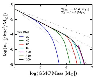
Figure 1: Case 1: Differential number density $n_{\rm cl}$ as a function of GMC mass, based on the fiducial calculation with CCC. The color corresponds to the time evolution. Note that the yellow line corresponds to $160$ Myr is almost fully overlapped by the black line for $200$ Myr, thus it is not visible on this plot. As a reference, we plot three gray straight lines; dot-dashed line fits the computed GMCMF slope ($\sim-1.7$), dashed line corresponds to the observed shallow slope whereas the dotted line shows the observed steep slope. The calculated GMCMF fits into the middle of the observed slope range.

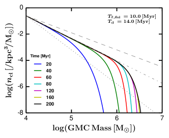
Figure 2: Case 2: Differential number density $n_{\rm cl}$ as a function of GMC mass, based on the fiducial calculation without CCC. The color corresponds to the time evolution. As a reference, we plot three gray straight lines; dot-dashed line fits the computed GMCMF slope ($\sim-1.7$), dashed line corresponds to the observed shallow slope whereas the dotted line shows the observed steep slope. The calculated GMCMF fits into the middle of the observed slope range. The similarity with Figure 1 indicates that CCC does not impact on the GMCMF slope significantly but modify the massive end.

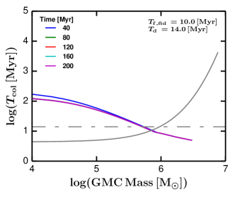
Figure 3: The three timescales as a function of GMC mass in Case 1. The gray solid line represents $T_{\rm f}$, the gray horizontal dot-dashed line corresponds to $T_{\rm d}$, and the colored lines show the time evolution of $T_{\rm col}$. Note that the three colored lines (i.e., the green line for $80$ Myr, the red line for $120$ Myr, and the cyan line for $160$ Myr) are overlapped by the purple line for $200$ Myr so that they are not visible on this plot. The figure indicates that GMC self-growth dominates in low-mass regime, but CCC deforms the GMCMF at its high-mass end where $T_{\rm col}$ is one order of magnitude smaller than self-growth timescale. Note that the gray line of $T_{\rm f}$ shown here has a factor difference from original $T_{\rm f}$ defined as Equation (4) (see Appendix E).

4.1 CCC contribution to the GMCMF slopes and massive ends

Figures 1 and 2 show our fiducial calculations (i.e., $T_{\rm f,fid}=10$ Myr, $T_{\rm d}=14$ Myr), which correspond to Case1 and Case2 respectively. The only difference between these two cases is whether the calculation includes the CCC terms (Figure 1) or not (Figure 2). Both computed GMCMFs demonstrate almost the same slope $-\alpha\sim-1.7$ (where $n_{\rm cl}\propto m^{-\alpha}$), which successfully fits into the middle of the observed range. This result indicates that CCC does not impact the GMCMF slope significantly whereas the shape of the massive end is modified by the relative importance between self-growth/dispersal and CCC.

To examine the relative contribution of CCC, we compute the collision timescale, $T_{\rm col}$, as:

$$T_{\rm col}=\frac{n_{\rm cl}(m)}{\left(\partial n_{\rm cl}/\partial t\right)_{\rm CCC}}\,,$$ (7)

where the denominator is the time evolution due to CCC:

$$\left(\frac{\partial n_{\rm cl}}{\partial t}\right)_{\rm CCC}= \frac{1}{2}\int_{0}^{\infty}\int_{0}^{\infty}K(m_{1},m_{2})n_{{\rm cl},1}n_{{\rm cl},2}$$ (8)

$$~{}~{}~{}~{}~{}~{}~{}~{}~{}~{}~{}~{}~{}~{}~{}~{}~{}~{}~{}\times\delta(m-m_{1}-m_{2}){\rm d}m_{1}{\rm d}m_{2}$$

$$-\int_{0}^{\infty}K(m,m_{2})n_{\rm cl}n_{{\rm cl},2}{\rm d}m_{2}\,.$$

Figure 3 shows the time evolution of computed $T_{\rm col}$, with $T_{\rm f}$ and $T_{\rm d}$ overplotted together. The figure indicates that the GMC mass growth is determined by GMC self-growth in low-mass regime where $T_{\rm f}$ ($\sim\mathcal{O}(1)$ Myr) is one order of magnitude shorter than $T_{\rm col}$ ($\sim\mathcal{O}(2)$ Myr), and is determined by CCC at the high-mass end where $T_{\rm col}$ ($\sim\mathcal{O}(1)$ Myr) becomes one order of magnitude smaller than $T_{\rm f}$ ($\sim\mathcal{O}(2)$ Myr). This indicates that the GMCMF slope in $m\lesssim 10^{5.5}\mbox{${\rm M_{\odot}}$}$ is well characterized by the combination of the GMC self-growth and dispersal. In the next section, we are going to focus only on the GMCMF slopes and will discuss the massive-end behavior in Section 4.3.

4.2 Characteristic Slope of the GMCMF

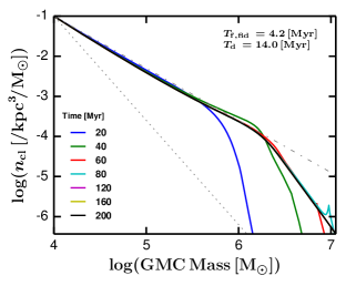
Figure 4: Case 3: Differential number density $n_{\rm cl}$ as a function of GMC mass, based on the calculation with $T_{\rm f,fid}=4.2$ Myr including CCC. The color corresponds to the time evolution. Note that the two colored lines (i.e., the purple line for $120$ Myr and the yellow line for $160$ Myr) are overlapped by the black line for $200$ Myr so that they are not visible on this plot. As a reference, we plot two gray straight lines; dot-dashed line corresponds to the observed GMCMF slope ($\sim-1.3$) in the arm regions, whereas the dotted line shows the observed steep slope in inter-arm regions. The agreement between the observed slope and the computed slope suggests that the arm regions typically have a shorter self-growth timescale, $T_{\rm f}\sim 4$ Myr. This is well characterized by the steady state solution without CCC shown in Equation (10). Again, the CCC effect is limited but modifies the GMCMF massive-end.

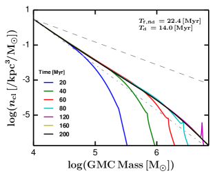
Figure 5: Case 4: Differential number density $n_{\rm cl}$ as a function of GMC mass, based on the calculation with $T_{\rm f,fid}=22.4$ Myr including CCC. The color corresponds to the time evolution. Note that the yellow line for $160$ Myr is overlapped by the black line for $200$ Myr, thus it is not visible on this plot. As a reference, we plot two gray straight lines; the dot-dashed line represents the observed steep slope ($\sim-2.6$) in the inter-arm regions, whereas the dashed line shows the observed shallow slope in the arm regions. Although the GMCMF shows the slope $\sim-2.2$ relatively shallower than the observed one $\sim-2.6$ due to the coagulation by CCC, the basic correspondence suggests that the inter-arm regions typically have a longer self-growth timescale $T_{\rm f}\sim 22$ Myr. This is well characterized by the steady state solution without CCC shown in Equation (10).

As shown in Section 4.1, CCC does not modify the GMCMF evolution significantly. Especially in lower mass range (e.g., $m<10^{5.5}\mbox{${\rm M_{\odot}}$}$) CCC does not affect the mass function, and hence our formulation can be rewritten without the CCC terms. Therefore, the evolution of differential number density of GMCs with mass $m$, $n_{\rm cl}$, is now simply given as:

$$\frac{\partial n_{\rm cl}}{\partial t}+\frac{\partial}{\partial m}\left(n_{\rm cl}\frac{m}{T_{\rm f}}\right)=-\frac{n_{\rm cl}}{T_{\rm d}}\,.$$ (9)

This formulation has been already (and originally) proposed by Inutsuka et al. (2015). One can obtain the steady state solution of this differential equation for $m\lesssim m_{\rm crit}$ with a constant $T_{\rm f}$ as:

$$n_{\rm cl}(m)=n_{0}\left(\frac{m}{\mbox{${\rm M_{\odot}}$}}\right)^{-1-\frac{T_{\rm f}}{T_{\rm d}}}\,,$$ (10)

where $n_{0}$ is the differential number density normalized at $m=1\mbox{${\rm M_{\odot}}$}$. This predicts that GMCMFs have slopes with a single exponent, which is well characterized by $-1-T_{\rm f}/T_{\rm d}$. Indeed, the computed GMCMF shows the slope consistent with this exponent $-1-T_{\rm f}/T_{\rm d}$ without CCC (see Figure 2), and in the lower mass ($m<10^{5.5}\mbox{${\rm M_{\odot}}$}$) part even in the case with CCC (see Figure 1).

To examine the validity of the $-1-T_{\rm f}/T_{\rm d}$ prediction, we conduct the calculation again by employing various $T_{\rm f}$. Figures 4 and 5 are the two representative results and both cases exhibit the slope well characterized by $-1-T_{\rm f}/T_{\rm d}$. Figure 4 employs a shorter formation timescale, $T_{\rm f,fid}=4.2$ Myr, and reproduces the observed shallow slope in arm regions. Similarly, Figure 5 shows the result with $T_{\rm f,fid}=22.4$ Myr, which reproduces the observed steep slope in inter-arm regions. Therefore, the arm regions presumably have a larger number of massive stars forming Hii regions and supernova remnants thus experience the recurrent supersonic compression twice more frequently than the fiducial case, and the inter-arm regions typically have a smaller number of massive stars thus experience less frequent supersonic compression, which results in about factor two longer formation timescale than the fiducial case. This may also explain the observed steep slope at outskirts of galaxies (e.g., the observed steep slope in the CO luminosity function in Galaxy M33; see Gratier et al. 2012) where star formation is less active compared with normal disk regions. Note that the above argument might be modified, if the effect of large-scale dynamics (e.g., interaction with shock waves or strong shear flows) may play an important role in the destruction of GMCs than the stellar feedback, especially in the outskirts of galaxies with prominent spiral structures.

Note that we here assume that the $T_{\rm d}$ variation between different regions is limited compared with the $T_{\rm f}$ variation. This is because $T_{\rm d}$ is basically independent of GMC mass as explained in Section 3.2 and also because observations suggest that the star formation efficiency is almost the same throughout the galactic disks in nearby galaxies (e.g., Schruba et al. 2011) and in the Galaxy (Izumi et al. in prep.). However, $T_{\rm d}$ might be longer in inter-arm regions compared with arm regions due to its less star forming activity where $T_{\rm d}$ can be up to $\sim 30$ Myr (the upper limit measured in M51 by Meidt et al. 2015), or might be a factor longer in smaller clouds $\lesssim 10^{5}\mbox{${\rm M_{\odot}}$}$ where it is invalid to apply our mass-independent assumption on the cloud destruction rate due to massive stars. The significance of $T_{\rm d}$ variation should be investigated more and we will leave this for future work.

Our results suggest that the variation of the GMCMF slopes are governed by $T_{\rm f}/T_{\rm d}$ diversity in different environment on galactic scales. We predict that future large radio surveys reveal that the GMCMFs have a single power-law exponent with which the ratio $T_{\rm f}/T_{\rm d}$ may be uniquely constrained.

4.3 Possible Modification in the Massive-end.

The shape of the GMCMF massive-end, typically $>10^{6}\mbox{${\rm M_{\odot}}$}$, is determined by the relative importance of GMC self-growth and CCC as shown in previous sections. The quantitative discussion involves many uncertainties from our modeling; for example, more detailed prescription for $\gamma$ is necessary for GMC self-growth (i.e., $T_{\rm f}$), and it is also required to model $T_{*}$ variation due to the drastic star formation invoked by CCC, which is inferred by observations in the Galaxy (c.f., Fukui et al. (2014); also see Section 6.1). These are beyond our current scope and to be discussed in our forthcoming paper.

Despite these limitation, our results indicate that, if CCC becomes effective, another structure may appear in the massive-end. This possibly explains the extra power-law feature observed in some regions (e.g., Material Arms) from PAWS survey (Colombo et al. 2014a).

5 Results 2: Fate of Dispersed Gas

5.1 Resurrecting factor

For all the time evolutions of the GMCMF we have shown in the previous sections, we assume that minimum-mass molecular clouds are continuously provided and the dispersed gas is removed from the system and never restored into the system.

However, in reality, dispersed gas should return to the ISM and become either seeds of newer generation of molecular clouds or mass accreting onto the pre-existing GMCs. To establish a complete picture of gas resurrecting processes in the ISM, we need to evaluate the fate of such dispersed gas. This aspiration requires detailed numerical simulations, ideally, three dimensional radiation magnetohydrodynamics simulations, which are however computationally too expensive to conduct. Instead in this article, we quantify the amount of dispersed gas by introducing the “resurrecting factor”, $\varepsilon_{\rm res}$, which is the mass fraction out of the total dispersed gas that are transformed to newer generation of minimum-mass GMCs. In Section 4, we artificially set the production rate of minimum-mass GMCs to keep its number density constant. Here instead, we evaluate this production rate due to gas resurrection as:

$$\left.\frac{\partial\left(n_{\rm cl}m\right)}{\partial t}\right|_{\rm res}=\varepsilon_{\rm res}\dot{M}_{\rm total,disp}\delta(m-m_{\rm min})\,,$$ (11)

where $\dot{M}_{\rm total,disp}$ is the total dispersed gas mass produced from the system per unit time, $m_{\rm min}$ is the minimum-mass of GMCs (i.e. $10^{4}\mbox{${\rm M_{\odot}}$}$ in this study), and $\delta$ is the Dirac delta function. By this definition, $\varepsilon_{\rm res}$ can be considered as the probability that dispersed gas becomes minimum-mass GMCs before they accrete onto the pre-existing GMCs and thus the $1-\varepsilon_{\rm res}$ fraction of dispersed gas are consumed for the self-growth of pre-existing GMCs if a GMCMF is in a steady state.

From now, we are going to focus only on steady state GMCMFs for simplicity. We may assume that the GMCMFs are quasi-steady in the Galaxy and nearby massive spiral galaxies because they presumably have already undergone active star formation phase at redshift $\sim 2$ and have relatively constant star formation activity at the present day (e.g. Madau & Dickinson 2014). Note that, although we have already proved that the CCC effect is limited, we fully solve Equation (1) including the CCC terms to compute the time evolution in all the following results. We mainly analyze Cases 5 to 8 in Table 3.1. The spikes and kinks that appear in the massive end (especially in Figs. 6,  9, and 11) are due to the numerical effect by the CCC turn-off procedure as explained in the second paragraph in Section 4.

5.2 Not All the Dispersed Gas are Consumed for Minimum-Mass GMC Creation

Here, we examine the fiducial timescales $T_{\rm f,fid}=10$ Myr and $T_{\rm d}=14$ Myr. First, we employ an extreme case where $\varepsilon_{\rm res}=1$; all the dispersed gas is consumed to form minimum-mass GMCs (Case 6) and Figure 6 shows the result. Initially the GMCMF exhibits slopes slightly steeper than $-1.7$ predicted by Equation (10). However the slope becomes more steepened in the low-mass regime and the total mass in the system keeps increasing so that the GMCMF does not show any steady state (see Figure 8). Therefore, the slopes are provisional and transitional. Indeed, the CCC becomes significantly effective after 60 Myr so that GMCs more massive than observed ones are instantly created after 60 Myr, which do not reproduce the observed GMCMFs.

The steepened slope observed in the low-mass end in Figure 6 appears due to overloading $\varepsilon_{\rm res}$, because pre-existing GMCs cannot acquire the excessive amount of resurrecting gas faster than a given self-growth timescale (in this case $10$Myr). To achieve a steady state with a shallower slope, we need to reduce $\varepsilon_{\rm res}$. Figure 7 shows a result with $\varepsilon_{\rm res}=0.09$ where we successfully reproduce a slope $-\alpha=-1.7$ throughout all the mass range and achieve a steady state GMCMF. To check the steadiness, we compute the total mass in the system as a function of time with various $\varepsilon_{\rm res}$ and Figure 8 shows the result. $\varepsilon_{\rm res}=0.09$ indicates that the GMCMF settle down on the steady state with a slight decrement in its total mass before the calculation ends at $200$ Myr. Contrarily, excessive input $\varepsilon_{\rm res}\gg 0.09$ leads to growth of the total mass and do not become steady by $200$Myr as, for example, already seen in Figure 6. Less input $\varepsilon_{\rm res}\ll 0.09$ leads to too much gas dispersal into the ISM and eventually decreases the total mass in the GMC phase, which would not reach any steady state before $200$Myr. In Section 5.5, we will investigate an analytical justification why $\varepsilon_{\rm res}\sim 0.09$ reaches a steady state and present the possible range of $\varepsilon_{\rm res}$ that provides a steady GMCMF.

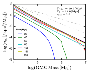
Figure 6: Case 5: Differential number density $n_{\rm cl}$ as a function of GMC mass including CCC with the fiducial timescales ($T_{\rm f,fid}=10$Myr and $T_{\rm d}=14$Myr) and with $\varepsilon_{\rm res}=1$. The color corresponds to the time evolution. As a reference, we plot three gray straight lines; the dot-dashed line is the slope $\sim-1.7$ predicted by Equation (10), the dotted line represents the observed steep slope ($\sim-2.6$) in the inter-arm regions, whereas the dashed line shows the observed shallow slope in the arm regions. The slope of the GMCMF is initially between $-1.7$ and $-2.6$ but becomes steepened and the total mass in the system keeps growing so that this does not reach any steady state (c.f., Figure 8). The kink in the massive-end at 40 Myr indicates the onset for the CCC-dominant phase. After 40 Myr, CCC becomes dominant and massive GMCs $>10^{7}\mbox{${\rm M_{\odot}}$}$ are continuously created, which is not consistent with observations, either. The steepened slope at the low-mass end appears due to overloading resurrection.

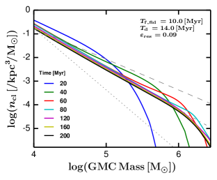
Figure 7: Case 6: Differential number density $n_{\rm cl}$ as a function of GMC mass including CCC with the fiducial timescales ($T_{\rm f,fid}=10$Myr and $T_{\rm d}=14$Myr) and with $\varepsilon_{\rm res}=0.09$. The color corresponds to the time evolution. As a reference, we plot three gray straight lines; the dot-dashed line is the slope predicted by Equation (10), the dotted line represents the observed steep slope ($\sim-2.6$) in the inter-arm regions, whereas the dashed line shows the observed shallow slope in the arm regions. The computed GMCMF successfully reproduces the fiducial slope $\sim-1.7$ predicted by Equation (10) and lands on a steady state as shown in Figure 8.

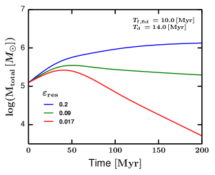
Figure 8: The total mass dependence on $\varepsilon_{\rm res}$ as a function of time with the fiducial setup ($T_{\rm f,fid}=10$ Myr and $T_{\rm d}=14$Myr). The different color represents the different $\varepsilon_{\rm res}$ from $0.0017$ to $0.2$. The GMCMF with $\varepsilon_{\rm res}=0.09$ reaches a steady state after 130 Myr elapse. $\varepsilon_{\rm res}=0.09$ reproduces the fiducial slope $-\alpha=-1.7$ as shown in Figure 7. Resurrecting more than $\varepsilon_{\rm res}=0.09$ (e.g., $0.2$ in this figure) increase the total mass in the system and the GMCMF would not reach any steady state. Similarly, resurrecting less than $\varepsilon_{\rm res}=0.09$ (e.g., $0.0017$ in this figure) eventually decrease the total mass in the system after 50 Myr. The steady resurrecting factor ($\sim 9$ per cent) is predictable, which we will explain in Section 5.5.

5.3 The Observed GMCMF Slopes in Arm Regions

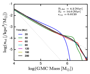
Figure 9: Case 7: Differential number density $n_{\rm cl}$ as a function of GMC mass including CCC with $T_{\rm f,fid}=4.2$ Myr and $\varepsilon_{\rm res}=0.0123$. The color corresponds to the time evolution. Note that the two colored lines (i.e., the purple line for $120$ Myr and the yellow line for $160$ Myr) are overlapped by the black line for $200$ Myr so that they are not visible on this plot. As a reference, we plot two gray straight lines; the dot-dashed line is the shallow slope ($\sim-1.3$) observed in the arm regions, and the dotted line represents the steep slope ($\sim-2.6$) observed in the inter-arm regions. The computed GMCMF successfully reproduces the shallow slope $\sim-1.3$ predicted by Equation (10) and reaches a steady state studied in Figure 10.

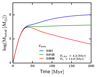
Figure 10: The total mass dependence on $\varepsilon_{\rm res}$ as a function of time with $T_{\rm f,fid}=4.2$ Myr The different color represents the different $\varepsilon_{\rm res}$ from $5.8\times 10^{-3}$ to $0.021$. The GMCMF with $\varepsilon_{\rm res}=0.0123$ reaches a steady state, $M_{\rm total}$, which is $\sim 4\times 10^{5}\mbox{${\rm M_{\odot}}$}$. $\varepsilon_{\rm res}=0.0123$ reproduces the shallow slope $-\alpha=-1.3$ as shown in Figure 9. Resurrecting more than $\varepsilon_{\rm res}=0.0123$ (e.g., $0.021$ in this figure) increase the total mass in the system. Similarly, resurrecting less than $\varepsilon_{\rm res}=0.0123$ (e.g., $5.8\times 10^{-3}$ in this figure) eventually decrease the total mass in the system after 60 Myr. The steady resurrecting factor ($\sim 1$ per cent) is predictable, which we will explain in Section 5.5.

We now focus on the shorter formation timescale $T_{\rm f,fid}=4.2$ Myr (Case 7) to examine what $\varepsilon_{\rm res}$ would reproduce the slopes observed in arm regions. Figure 9 shows the GMCMF time evolution with $\varepsilon_{\rm res}=0.0123$, which successfully reproduces the observed shallow slope $\sim-1.3$. Again, to check the steadiness, we compute the total mass in the system and Figure 10 shows the result with $\varepsilon_{\rm res}$ from $5.8\times 10^{-3}$ to $0.021$. The figure also confirms that $\varepsilon_{\rm res}=0.0123$ produces a steady state GMCMF. This factor $0.0123$ indicates that almost 99 per cent of dispersed gas are accreting onto and fueling pre-existing GMCs due to the multiple episodes of compression and that only 1 per cent of dispersed gas are turned to form newer generation of GMCs. This extreme fraction is expected due to massive GMCs; massive GMCs have larger surface area than less massive GMCs and collect large amount of diffuse ISM gas to grow. Therefore, small $\varepsilon_{\rm res}$, or large $1-\varepsilon_{\rm res}$, is likely to be realized in arm regions, which have many massive GMCs. We will discuss the range of $\varepsilon_{\rm res}$ around $0.0123$ that also keeps the GMCMF steady in Section 5.5.

5.4 The observed GMCMF Slopes in Inter-Arm Regions

We now focus on the longer formation timescale $T_{\rm f,fid}=22.4$ Myr (Case 8) to examine what $\varepsilon_{\rm res}$ would reproduce the slopes observed in inter-arm regions. Figure 11 shows the GMCMF time evolution with $\varepsilon_{\rm res}=0.45$. This GMCMF has its slope $\sim-2.4$, shallower than the observed slope $\sim-2.6$ due to the coagulation by CCC, which is also observed in Figure 5. We compute the total mass in the system and Figure 12 shows the result with $\varepsilon_{\rm res}$ from $0.133$ to $0.713$. The figure confirms that $\varepsilon_{\rm res}=0.45$ produces a steady state GMCMF. The initial condition is coincidently close enough to the steady state with $\varepsilon_{\rm res}=0.45$ thus the GMCMF with $\varepsilon_{\rm res}=0.45$ keep its total mass over the whole 200 Myr. This factor $0.45$ indicates that about 55 per cent of dispersed gas are accreting onto and fueling pre-existing GMCs due to the multiple episodes of compression and that 45 per cent of dispersed gas are turned to form newer generation of GMCs. This is naturally expected because the inter-arm regions do not contain many massive GMCs that may collect diffuse ISM to grow. We will discuss the range of $\varepsilon_{\rm res}$ around $0.45$ that also keeps the GMCMF steady in Section 5.5.

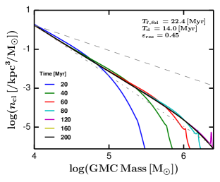
Figure 11: Case 8: Differential number density $n_{\rm cl}$ as a function of GMC mass including CCC with $T_{\rm f,fid}=22.4$ Myr and $\varepsilon_{\rm res}=0.45$. The color corresponds to the time evolution. Note that the yellow line for $160$ Myr is overlapped by the black line for $200$ Myr, thus it is not visible in this plot. As a reference, we plot two gray straight lines; the dot-dashed line is the steep slope ($\sim-2.6$) observed in the inter-arm regions, and the dashed line represents the shallow slope ($\sim-1.3$) observed in the arm regions. Although the computed GMCMF shows its slope $\sim-2.4$ slightly shallower than the observed value $-2.6$ due to the coagulation by CCC, this slope is basically predicted by Equation (10) and the GMCMF reaches a steady state studied in Figure 12.

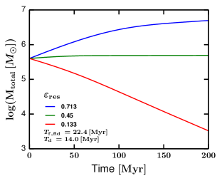
Figure 12: The total mass dependence on $\varepsilon_{\rm res}$ as a function of time with $T_{\rm f,fid}=22.4$ Myr. The different color represents the different $\varepsilon_{\rm res}$ from $0.133$ to $0.713$. The GMCMF with $\varepsilon_{\rm res}=0.45$ holds a steady state $M_{\rm total}$, which is $\sim 5\times 10^{5}\mbox{${\rm M_{\odot}}$}$, and reproduces the steep slope $-\alpha=-2.6$ as shown in Figure 11. The steadiness of the GMCMF with $\varepsilon_{\rm res}=0.45$ indicates that our initial condition setting only minimum-mass GMCs is close to the final steady state because smaller GMCs dominate the mass budget of the steepened GMCMF. Resurrecting more than $\varepsilon_{\rm res}=0.45$ (e.g., $0.713$ in this figure) increase the total mass in the system. Similarly, resurrecting less than $\varepsilon_{\rm res}=0.45$ (e.g., $0.133$ in this figure) decrease the total mass in the system. The steady resurrecting factor ($\sim 0.45$ per cent) is predictable, which we will explain in Section 5.5.

5.5 Analytical estimation on the resurrecting factors

In this section, we derive an analytical estimation for the steady state $\varepsilon_{\rm res}$ with its possible variation as a function of the GMCMF slope to explain the reason why the values we choose for the resurrecting factor in Sections 5.3 and 5.4 can successfully reproduce the observed variation of the GMCMFs. Here, we assume that the GMCMF in a mass range from $m_{\rm min}$ to $m_{\rm max}$ has a steady power-law state $n_{\rm cl}=Am^{-\alpha}$, where $A$ is a constant. We choose $m_{\rm min}=10^{4}\mbox{${\rm M_{\odot}}$}$ in our calculation (see Appendix D for the choice of $m_{\rm min}$ value), whereas $m_{\rm max}\approx m_{\rm trunc}$ as shown in the figures from our calculation by now.

To derive $\varepsilon_{\rm res}$ in a steady state GMCMF, we multiply $m$ by Equation (1) without the CCC term and modify the dispersal term into a form of $\partial/\partial m$:

$$\frac{\partial mn_{\rm cl}}{\partial t}+\frac{\partial}{\partial m}F(m)=0\,.$$ (12)

Here,

$$F(m)=\frac{m^{2}n_{\rm cl}}{T_{\rm f}(m)}-\int_{m_{\rm min}}^{m}\frac{mn_{\rm cl}{\rm d}m}{T_{\rm f}(m)}+\int_{m_{\rm min}}^{m}\frac{mn_{\rm cl}{\rm d}m}{T_{\rm d}}\,,$$ (13)

is the net mass flux at $m$ across the mass coordinate. Because we consider a steady state GMCMF at $m\leq m_{\rm trunc}$, $T_{\rm f}$ will be treated as a constant in the following analysis. Then $F(m)$ can be rewritten as:

$$F(m) =Am^{2-\alpha}\left(\frac{1}{T_{\rm f}}-\frac{1}{(2-\alpha)T_{\rm f}}+\frac{1}{(2-\alpha)T_{\rm d}}\right)$$ (14)

$$+Am_{\rm min}^{2-\alpha}\left(\frac{1}{(2-\alpha)T_{\rm f}}-\frac{1}{(2-\alpha)T_{\rm d}}\right)\,.$$

This mass flux is useful to evaluate the mass evolution in the system as we prove from now, and is also complementary with the original number density analysis because $\partial F(m)/\partial m=0$ reproduces the steady state slope predicted in Equation (10):

$$\alpha=1+\frac{T_{\rm f}}{T_{\rm d}}\,.$$ (15)

We introduce four characteristic quantities that control $\varepsilon_{\rm res}$; the incoming flux at the minimum-mass end, $F_{\rm in}$, the outgoing flux at the high-mass end, $F_{\rm out}$, the total mass growth per unit time by all the pre-existing GMCs, $\dot{M}_{\rm grow}$, and the total dispersed mass generated per unit time from the system, $\dot{M}_{\rm disp}$. They are given as:

$$F_{\rm in} = F(m_{\rm min})=m_{\rm min}^{2}n_{\rm cl}/T_{\rm f}\,,$$ (16)

$$F_{\rm out} = m_{\rm max}^{2}n_{\rm cl}/T_{\rm f}\,,$$ (17)

$$\dot{M}_{\rm grow} = \int_{m_{\rm min}}^{m_{\rm max}}\left(n_{\rm cl}m/T_{\rm f}\right){\rm d}m\,,$$ (18)

$$\dot{M}_{\rm disp} = \int_{m_{\rm min}}^{m_{\rm max}}\left(n_{\rm cl}m/T_{\rm d}\right){\rm d}m\,.$$ (19)

With these quantities, $F(m_{\rm max})$ corresponds to $F_{\rm out}-\dot{M}_{\rm grow}+\dot{M}_{\rm disp}$. In the steady state, $F(m)$ is independent of $m$. Thus $F(m_{\rm min})=F(m)=F(m_{\rm max})$ and this can be rewritten as:

$$F_{\rm in}=F_{\rm out}-\dot{M}_{\rm grow}+\dot{M}_{\rm disp}\,.$$ (20)

For massive GMCs, the power-law relation $n=Am^{-\alpha}$ is broken: the treatment is valid if we take $m_{\rm max}\approx m_{\rm trunc}$. For $m\gtrsim m_{\rm max}$, $T_{\rm f}$ is rapidly increases with mass and the dispersal becomes more important than the growth so that GMCs with $m\gtrsim m_{\rm max}$ are eventually dispersed. Therefore, $F_{\rm out}$ is interpreted as the mass dispersing rate at $m\geq m_{\rm max}$ and the total dispersal rate of GMCs is given by $\dot{M}_{\rm disp}+F_{\rm out}$. On the other hand, $F_{\rm in}$ means the formation rate of minimum-mass GMCs. Therefore, the resurrecting factor is given by

$$\varepsilon_{\rm res}=\frac{F_{\rm in}}{F_{\rm out}+\dot{M}_{\rm disp}}\,.$$ (21)

We consider that the GMCMF from $m_{\rm min}$ to $m_{\rm max}$ becomes in a steady state when $\varepsilon_{\rm res}=\varepsilon_{\rm res,std}$. Combined with Equation (20), $\varepsilon_{\rm res,std}$ is given as:

$$\varepsilon_{\rm res,std}$$ (22)

$$=\frac{F_{\rm in}}{F_{\rm in}+\dot{M}_{\rm grow}}$$

$$=\begin{cases}&\left\{1+\frac{1}{2-\alpha}\left[\left(\frac{m_{\rm max}}{m_{\rm min}}\right)^{2-\alpha}-1\right]\right\}^{-1}\quad(\text{for $\alpha\neq 2$})\,,\\ &\left[1+\ln(m_{\rm max}/m_{\rm min})\right]^{-1}\quad(\text{for $\alpha=2$})\,.\end{cases}$$

Table 5.5 shows the $\varepsilon_{\rm res,std}$ computed by Equation (22). Here, as a representative case of $m_{\rm max}<m_{\rm trunc}$, we opt to use $m_{\rm max}=10^{6.2}\mbox{${\rm M_{\odot}}$}$, which is also consistent with the truncated mass scale observed in our computed GMCMF (see also Fig. 13). Because $m_{\rm max}\gg m_{\rm min}$, Equation (22) can be simplified as

$$\varepsilon_{\rm res,std}$$ (23)

{(2-α)(mminmmax)2-α(for $\alpha<2$),[ln(mmax/mmin)]-1(for $\alpha=2$),α-2α-1(for $\alpha>2$).

Note that the accuracy of the approximation $m_{\rm max}<m_{\rm trunc}$ differs between cases, and thus the computed GMCMFs exhibit the resurrecting factors that slightly deviate by a factor $0.6-1.2$ from Equation (22) (i.e., Table 5.5).

Table 2: Estimated resurrecting factor as a function of growth timescale

Note. Predicted $\varepsilon_{\rm res,std}$ for three timescales: $T_{\rm f,fid}=4.2,10$, and $22.4$ Myr based on Equation (22). All the cases have a constant $T_{\rm d}=14$ Myr.

5.5.1 The range of the resurrecting factor

The integration of Equation (12) over $m$ from $m_{\rm min}$ to $m_{\rm max}$ results in

$$\frac{dM_{\rm total}}{dt} = F(m_{\rm min})-F(m_{\rm max})\,,$$ (24)

$$= F_{\rm in}-F_{\rm out}-\dot{M}_{\rm disp}+\dot{M}_{\rm grow}\,,$$

$$= \left(1-\frac{1}{\varepsilon_{\rm res}}\right)F_{\rm in}+\dot{M}_{\rm grow}\,.$$

where $M_{\rm total}$ is the total mass of GMCs from $m_{\rm min}$ to $m_{\rm max}$:

$$M_{\rm total}=\int_{m_{\rm min}}^{m_{\rm max}}mn_{\rm cl}{\rm d}m\,,$$ (25)

In the steady state, $dM_{\rm total}/dt=0$ and $\varepsilon_{\rm res}=\varepsilon_{\rm res,std}$. Therefore,

$$\dot{M}_{\rm grow}=-\left(1-\frac{1}{\varepsilon_{\rm res,std}}\right)F_{\rm in}\,.$$ (26)

The variation of $\varepsilon_{\rm res}$ changes $n_{\rm cl}$ and hence $\dot{M}_{\rm grow}$. However for simplicity, we here ignore the dependence of $\dot{M}_{\rm grow}$ on $\varepsilon_{\rm res}$ by considering $\varepsilon_{\rm res}\sim\varepsilon_{\rm res,std}$. From Equations (24) and (26), we obtain

$$\frac{dM_{\rm total}}{dt}=\left(\frac{1}{\varepsilon_{\rm res,std}}-\frac{1}{\varepsilon_{\rm res}}\right)F_{\rm in}\,.$$ (27)

If the GMCMF is steady and the total mass in the system $M_{\rm total}$ does not increase/reduce by factor $\beta$ within a certain timescale $T_{\rm steady}$,

$$\left|\frac{\beta M_{\rm total}}{\dot{M}_{\rm total}}\right|\gtrsim T_{\rm steady}\,.$$ (28)

Combining with Equation (26), the range of $\varepsilon_{\rm res}$ that leads to steady state becomes:

$$\left(1-\frac{\varepsilon_{\rm res,std}}{\varepsilon_{\rm res,std}+a}\right)\lesssim\frac{\varepsilon_{\rm res}}{\varepsilon_{\rm res,std}}\lesssim\left(1+\frac{\varepsilon_{\rm res,std}}{a-\varepsilon_{\rm res,std}}\right)\,,$$ (29)

where $a=F_{\rm in}T_{\rm steady}/(M_{\rm total}\beta)$.

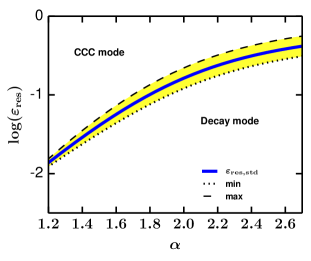
Figure 13: The range of the resurrecting factor, $\varepsilon_{\rm res}$, that sustain a steady GMCMF as a function of the GMCMF slope $-\alpha$ (i.e., $n_{\rm cl}(m)\propto m^{-\alpha}$). The thick solid blue line shows the estimated $\varepsilon_{\rm res,std}$ based on Equation (22). The dotted and dashed lines correspond to minimum and maximum of $\varepsilon_{\rm res}$ evaluated from Equation (29) with $\beta=0.5$, $T_{\rm steady}=100$ Myr, and $m_{\rm max}=10^{6.2}\mbox{${\rm M_{\odot}}$}$. $\varepsilon_{\rm res}$ increases with $\alpha$ and saturates when $\alpha$ becomes large (i.e., when the GMCMF has a steep slope) as expected from Equation (5.5). The variation of $\varepsilon_{\rm res}$ at a given $\alpha$ is less than one order of magnitude for all the $\alpha$ range. The GMCMFs with shallow slopes typically have $\varepsilon_{\rm res}=\mathcal{O}(10^{-2})$ whereas $\mathcal{O}(10^{-1})$ for steep slopes, which indicates that dispersed gas contributes more to the formation of newer generation GMC in inter-arm regions. The overloading resurrection more than maximum $\varepsilon_{\rm res}$ leads to the CCC-dominated regime. On the other hand, the GMCMF decays with the resurrection less than the minimum $\varepsilon_{\rm res}$.

Figure 13 shows the $\varepsilon_{\rm res,std}$ and $\varepsilon_{\rm res}$ variation based on Equations (22) and (29) with $m_{\rm max}=10^{6.2}\mbox{${\rm M_{\odot}}$}$. Here, we assume that the GMCMF can be steady and localized within the half galactic rotation (in a case of two spiral arms in a galactic disk) so that $T_{\rm steady}=100$ Myr and opt to use $\beta=0.5$. The figure shows that $\varepsilon_{\rm res}$ increase with $\alpha$. This trend is naturally expected because the inter-arm regions have less number of massive GMCs that can sweep up dispersed gas compared with the arm regions and dispersed gas easily produce minimum-mass GMCs when they experience multiple episodes of compression.

On the one hand, overwhelming resurrection more than the maximum $\varepsilon_{\rm res}$ increase the number density of GMCs, which ends up with the CCC-dominated regime after the long time elapse. On the other hand, the GMC number density decreases so that the GMCMF decays with resurrecting factor less than the minimum $\varepsilon_{\rm res}$.

5.5.2 Unseen gas

Up until now, we have shown that $\varepsilon_{\rm res}$ between $\mathcal{O}(0.01)$ to $\mathcal{O}(0.1)$ reproduces the observed GMCMF slope. The estimated face values themselves are important, but moreover, our results strongly suggest that understanding the fate of dispersed gas is inevitable to study the gas resurrecting processes in the ISM. The gas phases that are not well observed yet (e.g., CO-dark H₂ gas (Hosokawa & Inutsuka 2006; Tang et al. 2016; Xu et al. 2016) and optically thick Hi gas (Fukui et al. 2015a)) also come into play as well as usual CO-bright molecular gas. Three dimensional detailed magnetohydrodynamics simulation, for example, is required to understand the evolution of those unseen gas phases and to test whether it reproduces $\varepsilon_{\rm res}$ that we predict here.

6 DISCUSSION

6.1 CCC frequency and its impact

Our results indicate that CCC is limited only at the massive-end and does not alter the GMCMF time evolution significantly. This seems contrary to the CCC importance suggested by galactic simulations and observations, but is still consistent. The collision timescale typically varies from 1 to 100 Myr (see Figure 3), which is consistent with global galactic simulations (c.f., 25 Myr by Tasker & Tan (2009), 8 - 28 Myr by Dobbs et al. (2015)). Figure 3 shows that GMCs $>10^{6}\mbox{${\rm M_{\odot}}$}$ experience CCC much more frequently than GMCs $<10^{5}\mbox{${\rm M_{\odot}}$}$ as expected by the kernel function (Equation (6)). The lack of star cluster formation during CCC in our calculation generates many massive GMCs at the massive-end (c.f., Tasker & Tan 2009). However, we expect that such drastic star cluster formation take place only when larger GMCs collide each other (Fukui et al. 2014), which may affect the massive-end but not the slope. Therefore, our results indicate that inclusion of star cluster formation still does not impact the GMCMF slope significantly.

6.2 CCC-driven phase

In this section, we are going to investigate whether or not the cascade collisional coagulation alone can create a steady state GMCMF, which we investigated so far. Let us consider the mass flux as a function of GMC mass $m$. Suppose that the CCC kernel function has its mass dependence as $K\propto m^{p}$ and the resultant differential number density has a spectra $n\propto m^{-\alpha}$, the mass flux $F$ due to the cascade collisional coagulation becomes (c.f., Kobayashi & Tanaka 2010):

$$F\propto m^{3}n^{2}K\propto m^{-2\alpha+p+3}\,.$$ (30)

In a steady state, $F$ is constant across the whole mass range (i.e. $F\propto m^{0}$), therefore

$$p=2\alpha-3\,.$$ (31)

If the mass dependence of the kernel function has a variation with $p\in[-0.4,2.2]$ the observed slopes can be reproduced, which typically varies $-\alpha=-1.3--2.6$. Thus, the regions where the GMC number density is large (e.g., the Galactic Center) may form this type of CCC-driven GMCMF (c.f., Tsuboi et al. 2015). However, the collision alone reduce the number of minimum-mass GMCs quickly and also create infinitely massive GMCs. Therefore, we still need some proper prescription for the creation process at the low-mass end and the dispersal process at the high-mass end. We will investigate such a formulation in our upcoming paper. Also note that, the GMCMF may have the same slope when collision is not cascade but always occurs only with the minimum-mass bin, which we will also report in our forthcoming paper.

7 CONCLUSIONS AND SUMMARY

We have calculated the GMCMF time evolution by formulating a coagulation equation to reproduce and explain the possible origin of the observed variation in the GMCMF slopes. Our formulation is based on the paradigm that GMCs are created from magnetized WNM in galactic disks through multiple episodes of compression and such compression is driven by the network of expanding Hii regions and the late phase of supernova remnants.

Contrary to the previous works, we revealed that GMC self-growth overwhelm CCC. The GMCMF slope varies according to the diversity of GMC self-growth/dispersal timescales on galactic scales, which is essentially pointed out by Inutsuka et al. (2015); shallow slope with smaller ratio of growth/dispersal timescale. Our results demonstrate that future large radio surveys are capable of putting constraints on GMC self-growth and dispersal timescales in different environment on galactic scales.

We further include the gas resurrection process to regenerate GMCs after GMCs become dispersed due to star formation. The mass flux analysis under a steady state GMCMF assumption provides the analytical relation between the gas resurrecting factor and the GMC self-growth/dispersal timescales. Both the calculated GMCMF and the analytical relation agrees that typically over 90 % of the dispersed gas accrete onto the pre-existing GMCs in arm regions whereas only half in inter-arm regions. Typically, the arm regions have shorter formation timescale ($\sim 4$ Myr) and the inter-arm regions have longer formation timescale ($\sim 22$ Myr), indicating that the rate of massive star formation and/or supernovae is higher in arm regions than inter-arm regions.

The observational statistics for low mass GMCs are currently limited by completeness. Our results suggest that the GMCMF has a single power-law exponent in the mass range $<10^{5.5}\mbox{${\rm M_{\odot}}$}$, which may be revealed once observations start to resolve those smaller GMCs.

Due to its short evolution timescale ($\lesssim 100$ Myr), our formulation can be widely applied to the GMCMFs across galactic disks. Although galactic morphological diversity (e.g. elliptical and dwarf) is not explicitly described and currently beyond our scope, observed steep slope in elliptical galaxies (e.g. Utomo et al. 2015) indicates the potential capability of our formulation for various galactic morphologies. The CCC-dominated phase still remains to be studied and we are planning to report another formulation in our forthcoming paper that investigates the GMCMF in higher number density regions (such as the Galactic Center). Lastly, star formation phase of ISM is not studied yet in detail in the current article. Our formulation can be essentially extended to compute massive star and star cluster mass function and examine the Schmidt conjecture (i.e., Kennicutt-Schmidt law), which we would like to report as well in our forthcoming paper.

ACKNOWLEDGMENTS

We are grateful to the anonymous referee for providing thoughtful comments, which improved our manuscript in great details. MINK (15J04974), SI (23244027, 16H02160), and HK (26287101) are supported by Grants-in-Aid from the Ministry of Education, Culture, Sports, Science, and Technology of Japan. KH is supported by a grant from National Observatory of Japan. This work was supported by the Astrobiology Center Project of the National Institute of Natural Sciences (NINS) (grant Number AB271020). MINK thank Yasuo Fukui, Akihiko Hirota, Hidetoshi Sano, and Yusuke Hattori for educating us with observational backgrounds. MINK also appreciate Tsuyoshi Inoue, Hosokawa Takashi, Masahiro Nagashima, Martin Bureau, Ralph Schoenrich, Steven Longmore, Toby Moore, Jonathan Henshaw, Gary Fuller, Anthony Whitworth, Nicolas Peretto, Ana Duarte Cabral, Paul Clark, Cathie Clarke, Thomas Haworth, Chiaki Kobayashi, and Hua-Bai Li for fruitful discussion.

Appendix A VARIOUS EFFECTS

In the following appendices, we examine a variety of effects that modify the time evolution of the GMCMF; (i) Variation in the cross section, (ii) Variation in the relative velocities, (iii) Initial conditions, (iv) The choice for the minimum-mass GMC. The first two effects ((i) and (ii)) increase and decrease the rate for collisional coagulation. The setup variations fit into (iii) and (iv).

Appendix B Variation in the collision rate: cross section (geometrical structure and gravitational focusing) and relative velocity

In Section 3.3, we introduced the CCC kernel function, which has a correction factor $c_{\rm col}$. This $c_{\rm col}$ involves various effects; three main effects can be the geometrical structure, the gravitational focusing, and the relative velocity variation. We will explore these effects to verify that $c_{\rm col}$ has an order unity and $c_{\rm col}=1$ is enough approximation.

B.1 Geometrical structure

For simplicity, let us ignore the thickness of GMCs, which makes $c_{\rm col}$ a factor larger, and assume that GMCs always coagulate even when their peripheries alone touch each other.

Given that GMCs have a uniform column density $\Sigma_{\rm mol}$, the cross section for face-on collisional coagulation between GMCs whose masses are $m_{1}$ and $m_{2}$ ($m_{1}\geq m_{2}$), $\sigma_{\rm col\,peri\,1,2}$, is described as:

$$\sigma_{\rm col\,peri\,1,2} =\pi\left(R_{1}+R_{2}\right)^{2}$$ (32)

$$=\pi\left(\sqrt{\frac{m_{1}}{\pi\Sigma_{\rm mol}}}+\sqrt{\frac{m_{2}}{\pi\Sigma_{\rm mol}}}\right)^{2}$$

$$=\frac{\left(\sqrt{m_{1}}+\sqrt{m_{2}}\right)^{2}}{\Sigma_{\rm mol}}\,,$$

where $R_{1}$ and $R_{2}$ are the radii of GMCs with masses $m_{1}$ and $m_{2}$ respectively (see the left panel of Figure 14 for the schematic configuration). In this case, the correction factor becomes:

$$c_{\rm col}=\frac{\sigma_{\rm col\,peri\,1,2}}{\sigma_{\rm col\,1,2}}=1+\frac{2\sqrt{m_{1}}\sqrt{m_{2}}}{m_{1}+m_{2}}\,.$$ (33)

The second term gives the deviation from the unity and thus $c_{\rm col}$ has its maximum value $2$ when $m_{1}=m_{2}$. In reality, GMCs are less likely to coagulate together when their peripheries alone touch each other so that Equation (33) overestimates the collision frequency and $c_{\rm col}$ should be smaller by some factor. Therefore, we can assume $c_{\rm col}=1$ for simplicity.

The edge-on collision can be similarly evaluated. Supposed that GMCs collide with an angle $\theta$, the cross section becomes $2R_{1}\times 2R_{2}\times\sin\theta$ (see the right panel of Figure 14). $\sigma_{\rm col\,peri\,1,2}$ can be obtained by averaging this cross section over $\theta$:

$$\sigma_{\rm col\,peri\,1,2} =\frac{\int_{0}^{\pi}2R_{1}2R_{2}\sin\theta}{\pi}$$ (34)

$$=\frac{8}{\pi}R_{1}R_{2}$$

$$=\frac{8}{\pi^{2}\Sigma_{\rm mol}}\sqrt{m_{1}m_{2}}\,.$$

Therefore, the correction factor becomes:

$$c_{\rm col}=\frac{8}{\pi^{2}}\frac{\sqrt{m_{1}m_{2}}}{m_{1}+m_{2}}\,,$$ (35)

whose maximum is $0.57$ when $m_{1}=m_{2}$. Therefore, edge-on collision is less frequent than our fiducial cross section in Equation (6). Less frequent collision may impact on the shape of the massive end of the GMCMF. However, the slope calculated with overestimated $c_{\rm col}=1$ is not affected by CCC as shown in the figures by now. Therefore, for simplicity we can assume $c_{\rm col}=1$ even for the edge-on collision if we restrict ourselves to the slope of the GMCMF.

One caveat here is that we focus only on the collision in face-on and edge-on. The other orientations leads to the cross section smaller than the configuration we analyze here and would not greatly modify our GMCMF calculation results. Thus, we ignore such orientations for simplicity and left them for other works. Further investigation, especially three-dimensional hydrodynamics simulation, is needed.

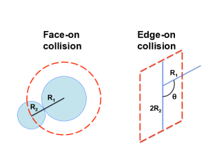
Figure 14: Schematic figure describing the geometrical configuration during cloud-cloud collisions (left: face-on collision; right: edge-on collision). GMCs have mass $m_{1}$ and $m_{2}$, radii $R_{1}$ and $R_{2}$ respectively. The red dashed area corresponds to the collisional cross section $\sigma_{\rm col\,peri\,1,2}$.

B.2 Gravitational focusing factor

During a close-by encounter, two GMCs experience gravitational attraction toward each other (i.e. gravitational focusing effect), which effectively enlarges the cross section so that the rate for collisional coagulation increases. To evaluate the gravitational focusing effect, let us consider an example where a GMC whose mass and radius are $m_{2}$ and $r_{2}$ initially flies at a speed $v_{\rm i}$ with an impact parameter $b$ with respect to another GMC with mass $m_{1}$ and radius $r_{1}$. Combining the angular momentum conservation and energy conservation, one can derive the ratio of the effective cross section $b^{2}$ against the area $(r_{1}+r_{2})^{2}$ as:

$$\frac{b^{2}}{\left(r_{1}+r_{2}\right)^{2}} =1+\Theta$$ (36)

$$=1+\frac{v_{\rm esc}^{2}}{v_{\rm i}^{2}}$$

$$=1+\frac{2{\rm G}(m_{1}+m_{2})}{(r_{1}+r_{2})v_{\rm i}^{2}}\,,$$

where $v_{\rm esc}$ is the escape velocity when the GMC peripheries touch each other. $\Theta$ is so called gravitational focusing factor, which characterize the relative increment of cross section due to gravitational attraction.

The condition where the gravitational focusing effect outnumbers the cross section would be $\Theta\gtrsim 1$. This condition with our ordinal assumption that GMCs have constant column density $\Sigma$ and $v_{\rm i}=10\,\mathrm{km\,s^{-1}}$ leads to:

$$\frac{m_{1}+m_{2}}{r_{1}+r_{2}}\gtrsim 1.16\times 10^{4}\,\mathrm{\mbox{${\rm M_{\odot}}$}\,pc^{-1}}$$ (37)

$$\Rightarrow\frac{m_{1}+m_{2}}{\sqrt{m_{1}}+\sqrt{m_{2}}}\gtrsim\frac{1.16\times 10^{4}\,\mathrm{\mbox{${\rm M_{\odot}}$}\,pc^{-1}}}{\sqrt{\pi\Sigma}}\,.$$

The left hand side of Equation (37) has its minimum when $m_{2}=0.17m_{1}$ and maximum when $m_{2}=m_{1}$. The most conservative estimation can be obtained by employing the maximum case $m_{2}=m_{1}$, which results in $m_{1}\gtrsim 5\times 10^{6}\mbox{${\rm M_{\odot}}$}$. This lower boundary may increase by another factor 3 to 5 because other collisions with $m_{2}<m_{1}$ generally exist and also $v_{\rm esc}\gtrsim\mathcal{O}(10)v_{\rm i}$ is required for CCC to overwhelm GMC self-growth/dispersal. Therefore, we can conclude that the gravitational focusing effect may be involved only in the mass range beyond $10^{7}\mbox{${\rm M_{\odot}}$}$. As shown in Sections 4 and after that, all the GMCMFs have already exhibited their well-defined slope below $10^{7}\mbox{${\rm M_{\odot}}$}$ thus treating the correction factor $c_{\rm col}=1$ is an enough approximation to compute the GMCMF slope correctly.

Note that our fiducial cross section is given as the sum of geometrical cross sections (i.e. $\pi r_{1}^{2}+\pi r_{2}^{2}$) rather than $\pi(r_{1}+r_{2})^{2}$ that we studied here. However, the former is smaller than the latter by only a factor one to two, thus the criterion $m_{1}\gtrsim 5\times 10^{6}\mbox{${\rm M_{\odot}}$}$ remains valid in our setup. Overall, the gravitational focusing effect can increase the cross section by some factors but we can still assume $c_{\rm col}=1$ for the mass range defining the GMCMF slope.

B.3 Relative velocity

The relative velocity between clouds is another component that may vary the collisional kernel. Because our model assumes that GMCs are swept up by expanding shells (e.g. Hii regions and supernova remnants), we expect that the relative velocity between GMCs is comparable to a typical shock expanding speed driven by the ionization-dissociation front (Hosokawa & Inutsuka 2006) and does not have any strong mass dependence. Even a simple setup can derive this estimation; the Rankine-Hugoniot relation (see Landau & Lifshitz 1959), for example, predicts that the velocity change across the shock front is described as $v_{2}=v_{1}\times\{(\gamma-1)\mathcal{M}_{1}^{2}+2\}\times((\gamma+1)\mathcal{M}_{1}^{2})^{-1}$, where $v_{1}$ and $v_{2}$ are the fluid speed in the pre-shock and post-shock regions respectively, $\mathcal{M}_{1}$ is the Mach number in the pre-shock region, and $\gamma$ is the polytropic index for the fluid. With a strong shock $\mathcal{M}\gg 1$, the cooling time can be longer than the dynamical time for the shock passing through a GMC, which leads to $\gamma>1$ rather than $\gamma=1$ even for a molecular cloud. Then the velocity change becomes $v_{2}=\mathcal{O}(0.1)\,v_{1}$ thus GMCs in the post-shock regions may have a relative velocity $\mathcal{O}(0.1)\times 10\,\mathrm{km\,s^{-1}}$. Semi-analytic studies also demonstrate that that a molecular cloud moves slowly than the shock itself (Iwasaki et al. 2011a, b), thus the GMC relative velocity would be somewhat smaller than $10\,\mathrm{km\,s^{-1}}$. Indeed, observations show that the mean intercloud dispersion in the Galaxy is a few $\mathrm{km\,s^{-1}}$ (Stark & Brand 1989; Stark & Lee 2005, 2006). Therefore, we opt to use $V_{\rm rel,0}=10\,\mathrm{km\,s^{-1}}$ irrespective of GMC mass, which may reduce $c_{\rm col}$ by a factor of a few. This compensates the increasing trend discussed in the previous sections so that $c_{\rm col}$ remains the order of unity.

Note that the shear motion in galactic disk would not outnumber the velocity dispersion produced by shocks. For example, supposed that two clouds at $R$ in a galactocentric coordinates have a separation of $d$ and the speed of the galactic rotation is $V_{\rm rot}$, then the shear speed can be estimated about $\sim V_{\rm rot}dR^{-1}$. With $V_{\rm rot}=200\,\mathrm{km\,s^{-1}}$, $d=100\,{\rm pc}$, and $R=8\mathrm{kpc}$ (e.g., solar neighbors), the shear speed becomes $2.5\,\mathrm{km\,s^{-1}}$. At the galactic centers with smaller $R$, the shear motion definitely contributes more to the GMC relative velocity, but the significance is non-trivial because GMCs are closer each other than disk regions so that may have smaller $d$. Because we now focus on disk regions, the shear motion does not alter the relative velocity appreciably in the conditions we present in the current article.

Appendix C Initial conditions

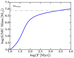
Figure 15: $T(m)=\int T_{\rm f}(m)/m\ {\rm d}m$ with $T_{\rm f,fid}=10$ Myr, which gives the typical self-growth timescales for GMCs that have not undergone CCC. A horizontal dash-dot line indicates $m_{\rm trunc}$. As expected from the exponential growth picture in Section 3.1, $T(m)$ logarithmically grows until GMCs acquire $m_{\rm trunc}/\gamma\sim 10^{6}\mbox{${\rm M_{\odot}}$}$ up to which $T_{\rm f}$ is almost constant (i.e., $T_{\rm f,fid}$). $T(m)$ rapidly increase beyond $m_{\rm trunc}/\gamma$ due to the $T_{\rm f}$ dependence on $m$ (see Equation (4)).

In general, the GMCMF time evolution may depend on the initial condition. To test the importance of the initial condition, we compute the time that is required for minimum-mass GMCs to grow to mass $m$ by Hi cloud accretion as:

$$T(m)=\int_{m_{\rm min}}^{m}\left[T_{\rm f}(m)/m\right]\,{\rm d}m\,.$$ (38)

This integration originates from our substitution $({\rm d}m/{\rm d}t)_{\rm self}=m/T_{\rm f}(m)$ in Section 3.1. Equation (38) suggests that GMCs grow exponentially in $m<m_{\rm trunc}$. We take the integration in Equation (38) and Figure 15 shows the result as a function of GMC mass. Note that, here, we include the $T_{\rm f}$ dependence on GMC mass (see Equation (4)). Therefore, the computed time exhibits a rapid increase at the massive end in Figure 15.

As shown in Figure 15, minimum-mass GMCs reach $10^{6}\mbox{${\rm M_{\odot}}$}$ within $100$ Myrs. Therefore, initial conditions for our calculation is erased typically less than one rotation of galactic disk and we expect that the observed GMCMF would not be affected significantly by the initial conditions. In case the initial condition is not influential in the resultant GMCMF, then formulation that depends on the initial condition (e.g., cosmological Press-Schechter formalism: Press & Schechter 1974) may not describe well the time evolution of the GMCMF.

Note that the GMCMF evolution can be modified in earlier stage if with the initial condition where very massive GMCs dominate the total mass of the system. However, based on the multiphase magnetohydrodynamics simulations (e.g. Inoue & Inutsuka 2008), multiple successive compression should first create smaller GMCs and cultivate them to massive ones, rather than produce very massive ones directly from WNM. Therefore, we opt to preset only minimum-mass GMCs at the beginning of our calculation (c.f. Appendix D for how to determine the minimum mass).

Appendix D The choice for the minimum-mass GMC

The concept of minimum-mass ($m_{\rm min}$) GMC is necessary to compute the GMCMF numerically. However, it is not trivial what value should be used as the “minimum” mass. Thus, to estimate this minimum value, let us consider a large hydrogen cloud. Given the mean number density in this cloud is $\sim 10^{2}\,\mathrm{cm^{-3}}$ and the visual extinction is 1 or larger due to the dust shielding to form molecular hydrogen (i.e. the total hydrogen column density $2\times 10^{21}\,\mathrm{cm^{-2}}$ (Bohlin et al. 1978; Rachford et al. 2009; Draine 2011)), the typical length for this type of hydrogen cloud is expected about $2\times 10^{21}/10^{2}=2\times 10^{19}\mathrm{cm}$. If we assume that the cloud has this length stretched at all the solid angles, then the total hydrogen mass in this cloud is given as:

$$\frac{4}{3}\pi\left(2\times 10^{19}\right)^{3}\times 10^{2}\times 2\mu m_{\rm H}$$ (39)

$$\simeq 2.6\times 10^{4}\mbox{${\rm M_{\odot}}$}\,.$$

ISM simulations (e.g., Inoue & Inutsuka 2012) also indicate that $10^{4}\mbox{${\rm M_{\odot}}$}$ is a typical minimum GMC created after 10 Myr. The minimum limit $\gtrsim 10^{4}\mbox{${\rm M_{\odot}}$}$ is consistent with the value observationally used (see Williams et al. 2000) as the definition of GMCs. Thus we opt to use $10^{4}\mbox{${\rm M_{\odot}}$}$ as the minimum-mass for GMCs.

However, the estimation by Equation (39) evaluates the minimum amount of total hydrogen but not molecular hydrogen alone. Therefore, in a static case where, for example, diffuse Hi gas extend around dense H₂ gas, the mass of dense H₂ gas can be half or less than Equation (39) prediction. Under a dynamical situation, turbulence stirs Hi and H₂ gas to break up H₂ cloud into smaller H₂ clouds whose mass can be smaller than that estimated by Equation (39). Moreover, if molecular gas self-shielding alone is effective when the dust is poor, the required total hydrogen column density can be smaller by a few orders of magnitude. Thus, even though we cannot specify the exact number, it maybe optimal to set somewhat smaller value than shown in Equation (39) as the minimum-mass of GMCs. We will investigate the minimum-mass choice further in our forthcoming paper, combining with the effect CO-dark H₂ gas and the $T_{\rm d}$ variation in low-mass less star-forming GMCs.

Note that, if the highest-density (star forming) H₂ regions have a filament structure (c.f. André et al. 2010; Molinari et al. 2010; Arzoumanian et al. 2011; Hill et al. 2011; Könyves et al. 2015), it is not trivial whether Hi gas sufficiently extend around those H₂ regions to sustain the column density condition ($2\times 10^{21}\,\mathrm{cm^{-2}}$). This needs to be studied further and left for future works.

Appendix E The mass flow timescale

$T_{\rm f}$ defined in Equation (1) are the timescales for the number flow. However $T_{\rm col}$ defined in Equation (7) is the timescale for the mass flow. To compare these two timescales, we need to convert $T_{\rm f}$ to the mass flow timescale, which can be evaluated as:

$$T_{\rm f,\,mass\,flow} =\left.mn_{\rm cl}\middle/\frac{\partial}{\partial m}\left(\frac{m^{2}n_{\rm cl}}{T_{\rm f}(m)}-\int_{m_{\rm min}}^{m}\frac{mn_{\rm cl}{\rm d}m}{T_{\rm f}(m)}\right)\right.$$ (40)

$$=\left.mn_{\rm cl}\middle/\left(\frac{\partial}{\partial m}\left(\frac{m^{2}n_{\rm cl}}{T_{\rm f}(m)}\right)-\frac{mn_{\rm cl}{\rm d}m}{T_{\rm f}(m)}\right)\right.\,,$$

(see Equation (12)). The gray line in Figure (3) shows this $T_{\rm f,\,mass\,flow}$ instead of $T_{\rm f}$.

References

- André et al. (2011) André, P., Men’shchikov, A., Könyves, V., & Arzoumanian, D. 2011, in IAU Symposium, Vol. 270, Computational Star Formation, ed. J. Alves, B. G. Elmegreen, J. M. Girart, & V. Trimble, 255–262
- André et al. (2010) André, P., Men’shchikov, A., Bontemps, S., et al. 2010, A&A, 518, L102
- Arzoumanian et al. (2011) Arzoumanian, D., André, P., Didelon, P., et al. 2011, A&A, 529, L6
- Audit & Hennebelle (2005) Audit, E., & Hennebelle, P. 2005, A&A, 433, 1
- Audit & Hennebelle (2008) Audit, E., & Hennebelle, P. 2008, in Astronomical Society of the Pacific Conference Series, Vol. 385, Numerical Modeling of Space Plasma Flows, ed. N. V. Pogorelov, E. Audit, & G. P. Zank, 73
- Bohlin et al. (1978) Bohlin, R. C., Savage, B. D., & Drake, J. F. 1978, ApJ, 224, 132
- Colombo et al. (2014a) Colombo, D., Hughes, A., Schinnerer, E., et al. 2014a, ApJ, 784, 3
- Colombo et al. (2014b) Colombo, D., Meidt, S. E., Schinnerer, E., et al. 2014b, ApJ, 784, 4
- Corder et al. (2008) Corder, S., Sheth, K., Scoville, N. Z., et al. 2008, ApJ, 689, 148
- Dobbs & Pringle (2013) Dobbs, C. L., & Pringle, J. E. 2013, MNRAS, 432, 653
- Dobbs et al. (2015) Dobbs, C. L., Pringle, J. E., & Duarte-Cabral, A. 2015, MNRAS, 446, 3608
- Draine (2011) Draine, B. T. 2011, Physics of the Interstellar and Intergalactic Medium
- Engargiola et al. (2003) Engargiola, G., Plambeck, R. L., Rosolowsky, E., & Blitz, L. 2003, ApJS, 149, 343
- Field et al. (1969) Field, G. B., Goldsmith, D. W., & Habing, H. J. 1969, ApJ, 155, L149
- Fukui et al. (2001) Fukui, Y., Mizuno, N., Yamaguchi, R., Mizuno, A., & Onishi, T. 2001, PASJ, 53, L41
- Fukui et al. (2015a) Fukui, Y., Torii, K., Onishi, T., et al. 2015a, ApJ, 798, 6
- Fukui et al. (2014) Fukui, Y., Ohama, A., Hanaoka, N., et al. 2014, ApJ, 780, 36
- Fukui et al. (2015b) Fukui, Y., Harada, R., Tokuda, K., et al. 2015b, ApJ, 807, L4
- Fukui et al. (2016) Fukui, Y., Torii, K., Ohama, A., et al. 2016, ApJ, 820, 26
- Gratier et al. (2012) Gratier, P., Braine, J., Rodriguez-Fernandez, N. J., et al. 2012, A&A, 542, A108
- Heitsch et al. (2005) Heitsch, F., Burkert, A., Hartmann, L. W., Slyz, A. D., & Devriendt, J. E. G. 2005, ApJ, 633, L113
- Heitsch et al. (2006) Heitsch, F., Slyz, A. D., Devriendt, J. E. G., Hartmann, L. W., & Burkert, A. 2006, ApJ, 648, 1052
- Heitsch et al. (2009) Heitsch, F., Stone, J. M., & Hartmann, L. W. 2009, ApJ, 695, 248
- Hennebelle & Audit (2007) Hennebelle, P., & Audit, E. 2007, A&A, 465, 431
- Hennebelle et al. (2007) Hennebelle, P., Audit, E., & Miville-Deschênes, M.-A. 2007, A&A, 465, 445
- Hennebelle & Pérault (1999) Hennebelle, P., & Pérault, M. 1999, A&A, 351, 309
- Hennebelle & Pérault (2000) —. 2000, A&A, 359, 1124
- Heyer & Dame (2015) Heyer, M., & Dame, T. M. 2015, ARA&A, 53, 583
- Heyer et al. (2001) Heyer, M. H., Carpenter, J. M., & Snell, R. L. 2001, ApJ, 551, 852
- Hill et al. (2011) Hill, T., Motte, F., Didelon, P., et al. 2011, A&A, 533, A94
- Hosokawa & Inutsuka (2006) Hosokawa, T., & Inutsuka, S.-i. 2006, ApJ, 646, 240
- Inoue & Inutsuka (2008) Inoue, T., & Inutsuka, S.-i. 2008, ApJ, 687, 303
- Inoue & Inutsuka (2009) —. 2009, ApJ, 704, 161
- Inoue & Inutsuka (2012) —. 2012, ApJ, 759, 35
- Inutsuka (2001) Inutsuka, S.-i. 2001, ApJ, 559, L149
- Inutsuka et al. (2015) Inutsuka, S.-i., Inoue, T., Iwasaki, K., & Hosokawa, T. 2015, A&A, 580, A49
- Iwasaki et al. (2011a) Iwasaki, K., Inutsuka, S.-i., & Tsuribe, T. 2011a, ApJ, 733, 16
- Iwasaki et al. (2011b) —. 2011b, ApJ, 733, 17
- Kawamura et al. (2009) Kawamura, A., Mizuno, Y., Minamidani, T., et al. 2009, ApJS, 184, 1
- Kennicutt & Evans (2012) Kennicutt, R. C., & Evans, N. J. 2012, ARA&A, 50, 531
- Kobayashi & Tanaka (2010) Kobayashi, H., & Tanaka, H. 2010, Icarus, 206, 735
- Koda et al. (2009) Koda, J., Scoville, N., Sawada, T., et al. 2009, ApJ, 700, L132
- Koda et al. (2011) Koda, J., Sawada, T., Wright, M. C. H., et al. 2011, ApJS, 193, 19
- Koda et al. (2012) Koda, J., Scoville, N., Hasegawa, T., et al. 2012, ApJ, 761, 41
- Könyves et al. (2015) Könyves, V., André, P., Men’shchikov, A., et al. 2015, A&A, 584, A91
- Körtgen & Banerjee (2015) Körtgen, B., & Banerjee, R. 2015, MNRAS, 451, 3340
- Koyama & Inutsuka (2000) Koyama, H., & Inutsuka, S.-I. 2000, ApJ, 532, 980
- Koyama & Inutsuka (2002) Koyama, H., & Inutsuka, S.-i. 2002, ApJ, 564, L97
- Kramer et al. (1998) Kramer, C., Stutzki, J., Rohrig, R., & Corneliussen, U. 1998, A&A, 329, 249
- Kwan (1979) Kwan, J. 1979, ApJ, 229, 567
- Landau & Lifshitz (1959) Landau, L. D., & Lifshitz, E. M. 1959, Fluid mechanics
- Madau & Dickinson (2014) Madau, P., & Dickinson, M. 2014, ARA&A, 52, 415
- McKee & Ostriker (1977) McKee, C. F., & Ostriker, J. P. 1977, ApJ, 218, 148
- Meidt et al. (2015) Meidt, S. E., Hughes, A., Dobbs, C. L., et al. 2015, ApJ, 806, 72
- Molinari et al. (2010) Molinari, S., Swinyard, B., Bally, J., et al. 2010, A&A, 518, L100
- Nakamura et al. (2012) Nakamura, F., Miura, T., Kitamura, Y., et al. 2012, ApJ, 746, 25
- Onishi et al. (1999) Onishi, T., Kawamura, A., Abe, R., et al. 1999, PASJ, 51, 871
- Pety et al. (2013) Pety, J., Schinnerer, E., Leroy, A. K., et al. 2013, ApJ, 779, 43
- Press & Schechter (1974) Press, W. H., & Schechter, P. 1974, ApJ, 187, 425
- Rachford et al. (2009) Rachford, B. L., Snow, T. P., Destree, J. D., et al. 2009, ApJS, 180, 125
- Rice et al. (2016) Rice, T. S., Goodman, A. A., Bergin, E. A., Beaumont, C., & Dame, T. M. 2016, ApJ, 822, 52
- Rosolowsky et al. (2003) Rosolowsky, E., Engargiola, G., Plambeck, R., & Blitz, L. 2003, ApJ, 599, 258
- Rosolowsky et al. (2007) Rosolowsky, E., Keto, E., Matsushita, S., & Willner, S. P. 2007, ApJ, 661, 830
- Roy et al. (2015) Roy, A., André, P., Arzoumanian, D., et al. 2015, A&A, 584, A111
- Salpeter (1955) Salpeter, E. E. 1955, ApJ, 121, 161
- Schinnerer et al. (2013) Schinnerer, E., Meidt, S. E., Pety, J., et al. 2013, ApJ, 779, 42
- Schinnerer et al. (2017) Schinnerer, E., Meidt, S. E., Colombo, D., et al. 2017, ArXiv e-prints (accepted to ApJ), arXiv:1701.02184
- Schruba et al. (2011) Schruba, A., Leroy, A. K., Walter, F., et al. 2011, AJ, 142, 37
- Scoville & Hersh (1979) Scoville, N. Z., & Hersh, K. 1979, ApJ, 229, 578
- Stark & Brand (1989) Stark, A. A., & Brand, J. 1989, ApJ, 339, 763
- Stark & Lee (2005) Stark, A. A., & Lee, Y. 2005, ApJ, 619, L159
- Stark & Lee (2006) —. 2006, ApJ, 641, L113
- Tacconi et al. (2010) Tacconi, L. J., Genzel, R., Neri, R., et al. 2010, Nature, 463, 781
- Tachihara et al. (2000) Tachihara, K., Mizuno, A., & Fukui, Y. 2000, ApJ, 528, 817
- Tan (2000) Tan, J. C. 2000, ApJ, 536, 173
- Tang et al. (2016) Tang, N., Li, D., Heiles, C., et al. 2016, A&A, 593, A42
- Tasker & Tan (2009) Tasker, E. J., & Tan, J. C. 2009, ApJ, 700, 358
- Tomisaka (1986) Tomisaka, K. 1986, PASJ, 38, 95
- Torii et al. (2015) Torii, K., Hasegawa, K., Hattori, Y., et al. 2015, ApJ, 806, 7
- Tosaki et al. (2016) Tosaki, T., Kohno, K., Harada, N., et al. 2016, ArXiv e-prints (in press at PASJ), arXiv:1612.00948
- Tsuboi et al. (2015) Tsuboi, M., Miyazaki, A., & Uehara, K. 2015, PASJ, 67, 90
- Utomo et al. (2015) Utomo, D., Blitz, L., Davis, T., et al. 2015, ApJ, 803, 16
- Valdivia et al. (2016) Valdivia, V., Hennebelle, P., Gérin, M., & Lesaffre, P. 2016, A&A, 587, A76
- Vázquez-Semadeni et al. (2006) Vázquez-Semadeni, E., Ryu, D., Passot, T., González, R. F., & Gazol, A. 2006, ApJ, 643, 245
- Walder & Folini (1998a) Walder, R., & Folini, D. 1998a, A&A, 330, L21
- Walder & Folini (1998b) —. 1998b, Ap&SS, 260, 215
- Williams et al. (2000) Williams, J. P., Blitz, L., & McKee, C. F. 2000, Protostars and Planets IV, 97
- Williams & McKee (1997) Williams, J. P., & McKee, C. F. 1997, ApJ, 476, 166
- Wolfire et al. (1995) Wolfire, M. G., Hollenbach, D., McKee, C. F., Tielens, A. G. G. M., & Bakes, E. L. O. 1995, ApJ, 443, 152
- Wolfire et al. (2003) Wolfire, M. G., McKee, C. F., Hollenbach, D., & Tielens, A. G. G. M. 2003, ApJ, 587, 278
- Xu et al. (2016) Xu, D., Li, D., Yue, N., & Goldsmith, P. F. 2016, ApJ, 819, 22
- Yonekura et al. (1997) Yonekura, Y., Dobashi, K., Mizuno, A., Ogawa, H., & Fukui, Y. 1997, ApJS, 110, 21