Imprints of Zero-Age Velocity Dispersions and Dynamical Heating on the Age-Velocity dispersion Relation

Abstract

Observations of stars in the the solar vicinity show a clear tendency for old stars to have larger velocity dispersions. This relation is called the age-velocity dispersion relation (AVR) and it is believed to provide insight into the heating history of the Milky Way galaxy. Here, in order to investigate the origin of the AVR, we performed smoothed particle hydrodynamic simulations of the self-gravitating multiphase gas disks in the static disk-halo potentials. Star formation from cold and dense gas is taken into account, and we analyze the evolution of these star particles. We find that exponents of simulated AVR and the ratio of the radial to vertical velocity dispersion are close to the observed values. We also find that the simulated AVR is not a simple consequence of dynamical heating. The evolution tracks of stars with different epochs evolve gradually in the age-velocity dispersion plane as a result of: (1) the decrease in velocity dispersion in star forming regions, and (2) the decrease in the number of cold/dense/gas as scattering sources. These results suggest that the AVR involves not only the heating history of a stellar disk, but also the historical evolution of the ISM in a galaxy.

1 Introduction

It is well known that the velocity dispersion of stars in the solar vicinity increases with stellar age. This is called the age–velocity dispersion relation (hereafter AVR). Strömberg (1946) and Spitzer & Schwarzschild (1951) were the first to investigate the association between stellar velocity dispersion and spectral types, and then they discovered this relation. Subsequent observations (Nordström et al., 2004; Seabroke & Gilmore, 2007; Holmberg et al., 2007, 2009; Aumer & Binney, 2009; Just & Jahreiß, 2010; Sharma et al., 2014) confirmed the existence of the AVR with much larger samples. According to these observations, this relation is well fitted by a single power-law function for both the radial ($\sigma_{R}$) and vertical ($\sigma_{z}$) directions:

$$\sigma\propto\tau^{\beta},$$ (1)

where $\sigma$ represents $\sigma_{R}$ or $\sigma_{z}$ and $\tau$ is the age of the star. The power-law index, $\beta$, is $0.3$–$0.5$ with certain errors (See table 8 of Sharma et al. (2014)). The index for the radial direction is slightly smaller than that for the vertical direction. However, it is not clear whether this difference is real or not. $\sigma_{z}/\sigma_{R}\sim 0.5$ has also been ascertained by observations (Dehnen & Binney, 1998).

Some secular heating processes and/or time evolution in the disk play crucial roles in establishing the AVR (e.g., Wielen (1977); Freeman & Bland-Hawthorn (2002); Bland-Hawthorn & Gerhard (2016) for reviews), since the older stars tend to have larger velocity dispersions. There are a number of scenarios for the origin of the AVR: heating by giant molecular clouds (GMCs; Spitzer & Schwarzschild (1951, 1953); Kokubo & Ida (1992)), by transient spiral arms (Carlberg & Sellwood, 1985; De Simone et al., 2004), by the combination of GMCs and spiral arms (Carlberg, 1987; Jenkins & Binney, 1990), by halo black holes (Lacey & Ostriker, 1985; Hänninen & Flynn, 2002), or by minor mergers (Toth & Ostriker, 1992; Walker et al., 1996; Huang & Carlberg, 1997). Until now, there has been no consensus about the primary source of the AVR. In table 1, we summarize the theoretical predictions of velocity dispersions in both the radial and vertical directions. All of the above processes are key features of galaxy formation. Thus, understanding the origin of the AVR is essential in order to advance our understanding of galaxy formation.

Table 1: Velocity dispersions predicted by the theoretical models. We summarize the models referring to AVRs and its exponents. Note that, in the case of minor mergers, only the amount of the increase of velocity dispersions are shown.

	heating source	velocity dispersion $\sigma$
Spitzer & Schwarzschild (1953)	GMC	$\sigma_{\rm mean}\propto\tau^{1/3}$
Kokubo & Ida (1992)	GMC	$\sigma_{R}\propto\tau^{0.25}$, $\sigma_{z}\propto\tau^{0.25}$
Hänninen & Flynn (2002)	GMC	$\sigma_{R}\propto\tau^{0.21}$, $\sigma_{z}\propto\tau^{0.26}$
De Simone et al. (2004)	spiral arm	$\sigma_{R}\propto\tau^{0.20{\rm\mathchar 45\relax}0.60}$
		(depending on spiral properties)
Jenkins & Binney (1990)	GMC & spiral arm	$\sigma_{R}\propto\tau^{0.5}$, $\sigma_{z}\propto\tau^{0.3}$
Hänninen & Flynn (2002)	halo black hole	$\sigma_{R}\propto\tau^{0.50}$, $\sigma_{z}\propto\tau^{0.50}$
Walker et al. (1996)	minor merger	incease by $\delta\sigma\sim(10,8,8)~{}{\rm kms^{-1}}$ at solar radius
Huang & Carlberg (1997)	minor merger	$\sigma_{z}$ increase by a few – dozens %
		(depending on satellite mass and falling angle)

Here, we mainly focus on the contribution of GMCs to the formation of the AVR. Some previous studies investigated the effect of gravitational scattering by GMCs on the velocity dispersions of stars. Kokubo & Ida (1992) calculated stellar orbits under the influence of the gravitational potential of GMCs, and they found that the evolution of velocity dispersion could be divided into two phases. In the early phase, the evolution of the velocity dispersion is proportional to $\exp(\tau)$, while in the late phase, it is proportional to $\tau^{0.25}$. Hänninen & Flynn (2002) performed $N$-body simulations of the stellar disk involving GMCs modeled by spherical mass distributions of uniform density. They found that the radial and vertical velocity dispersions are proportional to $\tau^{0.21}$ and $\tau^{0.26}$, respectively. This is consistent with the prediction from the simplified model of Kokubo & Ida (1992), but the expected values of velocity dispersions are somehow different from those obtained from observations. Hence, gravitational scattering by GMCs is not considered a primary source of the AVR. However, the models used above show significant room for improvement. For instance, they did not take into account gas dynamics, they did not model GMCs as realistic structures, and they did not consider star-formation processes. Aumer et al. (2016b) and Aumer et al. (2016a) performed controlled $N$-body simulations of disk galaxies to investigate the disk growth. In these simulations, they study the contribution of GMCs to the disk growth by using massive $N$-body particles which represent GMCs. They found that the efficiency of GMC heating depends on the fraction of disk mass residing in the GMC. Models that are more realistic are necessary to conclude whether or not GMC heating is important in the establishment of the AVR.

Recently, some zoom-in cosmological simulations have been used to derive numerical estimations of the AVRs. Brook et al. (2012) carried out $N$-body/smoothed particle hydrodynamics (SPH) simulations with the mass and spatial resolutions of $7300~{}M_{\odot}$ and $155~{}{\rm pc}$. They showed that old stars that have larger velocity dispersion were born at lower radii and are kinematically hotter than those born at a later time. Martig et al. (2014) used adaptive mesh refinement code RAMSES (Teyssier, 2002) and they showed that AVR is not determined by the stellar velocity dispersion at birth time, but is the result of subsequent heating. Furthermore, House et al. (2011) investigated the variations of AVR using different modeling techniques. Grand et al. (2016) used the state-of-the-art simulation code, AREPO (Springel, 2010), for their zoom-in simulations and reported that they obtained an AVR that is consistent with the observed AVR. While all studies showed power-law-like AVRs, we note that their simulations are insufficient to disclose the origin of the AVR because of the limited numerical resolutions (the force resolution is $\geq 100~{}{\rm pc}$), which is larger than the thickness of the molecular gas disk ($48$–$160~{}{\rm pc}$) in the Milky Way galaxy (Nakanishi & Sofue, 2006). Some models did not directly solve the low temperature ($\lesssim 100$ K) and high-density regions ($\gtrsim 100~{}\rm cm^{-3}$) that mimic GMCs. In addition, the origin of the AVR is not well investigated in these studies.

In this paper, we find out the origin of the AVR by using high-resolution $N$-body/SPH simulations. Instead of doing the cosmological simulations, we adopt an idealized model in which only gas and stars formed from cold and dense gas are solved. The halo and (the main body of) the stellar disk are expressed by static potentials. This approximation allows us to use high mass and spacial resolutions, such as $6000~{}M_{\odot}$ and $10~{}{\rm pc}$. As a trade-off, we cannot include the contribution of the spiral arms at present, but this will constitute the next step of this study and we will investigate it in a forthcoming paper.

The structure of this paper is as follows. In §2, we describe the initial conditions of our simulations and our numerical methods. We present the evolution of the simulated galactic disk and AVRs in our simulation in §3. Heating rates are also discussed in this section. Finally, in §4, we show the summary of our results and its implications for the history of the formation and evolution of the Milky Way galaxy.

2 Models and Methods

Our three dimensional (3D) $N$-body/SPH simulations conducted in this study were performed using the ASURA-2 (Saitoh & Makino, 2009, 2010). We investigated the AVR for stellar particles formed from SPH particles moving within a static halo and disk potential.

2.1 Galaxy Model

In order to concentrate on the contribution of the clumpy interstellar medium (ISM) to the stellar velocity dispersion, we solve the evolution of the gas with high resolutions. For this purpose, here we assume that the halo and the main body of the stellar disk are described by fixed potentials. This modeling is identical to that of Saitoh et al. (2008).

We assume that the dark matter halo follows the Navarro-Frenk-White (NFW) profile (Navarro et al., 1997), which is expressed as

$$\rho_{\rm halo}(x) = \frac{\rho_{\rm c}}{x(1+x)^{2}},$$ (2)

$$x = \frac{r}{r_{\rm s}},$$ (3)

where $\rho_{\rm c}$ and $r_{\rm s}$ are the characteristic density and a scale radius of this profile, respectively. We assume that $\rho_{c}=4.87\times 10^{6}~{}M_{\odot}~{}{\rm kpc^{-3}}$ and $r_{\rm s}=21.5~{}{\rm kpc}$.

The potential of the stellar disk is described by the Miyamoto-Nagai model (Miyamoto & Nagai, 1975):

$$\rho_{\ast}(R,z) = \frac{M_{\ast}z_{\ast}^{2}}{4\pi}\times$$ (4)

$$\frac{R_{\ast}R^{2}+(R_{\ast}+3\sqrt{z^{2}+z_{\ast}^{2}})(R_{\ast}+\sqrt{z^{2}+z_{\ast}^{2}})^{2}}{[R^{2}+(R_{\ast}+\sqrt{z^{2}+z_{\ast}^{2}})^{2}]^{5/2}(z^{2}+z_{\ast}^{2})^{3/2}},$$

where $M_{\ast}$, $R_{\ast}$, and $z_{\ast}$ are the stellar disk mass, the scale radius and the scale height, respectively. We use $M_{\ast}=4\times 10^{10}~{}M_{\odot}$, $R_{\ast}=3.5~{}{\rm kpc}$, and $z_{\ast}=400~{}{\rm pc}$.

Initially, the gas disk has simple exponential and Gaussian distributions in the radial and vertical directions. The scale radius and the scale height of the gas distribution are set to $7~{}{\rm kpc}$ and $400~{}{\rm pc}$, respectively. Figure 1 shows the averaged rotation curve of gas particles at the initial conditions. The total mass of the gas disk is $6\times 10^{9}M_{\odot}$, and we use 1 million SPH particles to express this gas disk. Hence, the mass of each SPH particle is $6000~{}M_{\odot}$. The gravitational softening length is set to $10~{}{\rm pc}$.

Figure 1: Initial rotational velocity as a function of radius. $\langle v_{\phi}\rangle$ is the average azimuthal velocity of initial SPH particles located in each radial bin. We apply a width of $0.1~{}{\rm kpc}$ to the radial bins.

2.2 Methods

We solve the evolution of gas and star particles in the halo and disk potential using our $N$-body/SPH code, ASURA-2 (Saitoh & Makino, 2009, 2010). The numerical technique is almost the same as those used in above papers, but with slight updates. We now briefly describe our method.

The self-gravity among the gas and star particles is calculated by the tree with the GRAvity PipE (GRAPE) method (Makino, 1991). The opening angle is set to 0.5 and only monopole moment is considered. In order to accelerate the computation, we adopt the Phantom-GRAPE library (Tanikawa et al., 2013), which is a software emulator of GRAPE.

The gas dynamics are solved by using SPH (Lucy, 1977; Gingold & Monaghan, 1977; Monaghan, 1992). The cubic-spline kernel function is utilized. For the first space derivative of the kernel, Thomas & Couchman’s modification is employed (Thomas & Couchman, 1992). The number of neighboring particles for each SPH particle is kept within $32\pm 2$ in the support radius of the kernel. The shock is handled with an artificial viscosity term proposed by Monaghan (1997). The viscosity coefficient is set to 1.0. We also introduce the Balsara limiter in order to reduce the unwanted angular momentum transfer (Balsara, 1995).

The time integration is conducted by a second order scheme (see appendix A in Saitoh & Makino (2016)). For SPH particles, we use the FAST scheme so that we can accelerate the time-integration in supernova (SN)-heated regions by using different time-steps for gravitational and hydrodynamical interactions (Saitoh & Makino, 2010) and the time-step limiter so that we can follow the shocked region correctly (Saitoh & Makino, 2009).

In simulations in this paper, we adopt the radiative cooling, star formation, and type II supernovae (SNe) feedback. The radiative cooling of the gas is solved by assuming an optically thin cooling function, $\Lambda(T,f_{\rm H2},G_{0})$, for a wide temperature range of $20~{}{\rm K}<T<10^{8}~{}{\rm K}$ (Wada et al., 2009) For simplicity, we fix the molecular hydrogen fraction at $f_{\rm H2}=0.5$, and the far-ultraviolet intensity is normalized to the solar neighborhood $G_{0}=1$. We do not have to use the artificial pressure floor method, which is highlighted in Saitoh et al. (2006) and Robertson & Kravtsov (2008). Star formation is modeled in a probabilistic manner following the Schmidt law (e.g., Katz (1992); Saitoh et al. (2008)). An SPH particle which satisfies the following three conditions, (1) $n_{\rm H}>100~{}{\rm cm^{-3}}$; (2) $T<100~{}{\rm K}$; and (3) $\nabla\cdot\mathbf{v}<0$, spawns a star particle with the Salpeter initial mass function (Salpeter, 1955) and is within the mass range of $0.1~{}M_{\odot}<m_{\rm\star}<100~{}M_{\odot}$. As an early stellar feedback, the ${\rm H_{II}}$-region feedback using a Stromgren volume approach (Baba et al., 2017) is employed. The energy feedback from type II SNe is implemented. Each SN releases $10^{51}~{}{\rm erg}$, and this energy is injected into the surrounding ISM. We adopt the probabilistic manner of Okamoto et al. (2008) to evaluate the injection time.

3 Results

We analyze the AVR in the simulations and investigate its evolution in §3.1. We then discuss the origins of AVR evolution in §3.2.

Before presenting the details of the AVR and its origin, we first explain the global evolution of our galaxies. Figure 2 shows the evolution of our simulated galaxies. The upper and lower panels show overviews and close-up views of the gas density on the galactic plane ($z=0$). From the close-up views of the gas density, we can see rich inhomogeneous structures of the ISM. These structures are induced by our modeling with high resolution (Saitoh et al., 2008). From $t=1$ – $3~{}{\rm Gyr}$, the contrast of the gas density decreases because of the gas consumption due to star formation. This implies that the primary source heating the disk stars decreases with increasing time in our simulation. We discuss the relation between the contrast of the gas density and heating rate in §3.2.2.

The high-density regions exceed the star formation threshold density (i.e. $n_{\rm H}>100~{}\rm cm^{-3}$) Therefore, stars are formed in these high-density regions when the other two star-formation conditions are satisfied. Figure 3 shows the evolution of stellar surface density. The stellar surface density distribution maps show no strong spiral arms developed by stellar dynamical mechanisms such as the swing-amplification (Toomre, 1981) and non-linear interactions between wakelets (Kumamoto & Noguchi, 2016). As the skeletal structure of the disk is constructed of the smoothed and axisymmetric Miyamoto-Nagai potential, it is difficult to enhance the spiral arms and a bar in this model; thus, it has a flocculent structure.

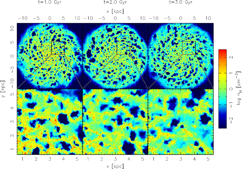
Figure 2: The gas density on the galactic plane ($z=0$) at $t=1$, $2$, and $3~{}{\rm Gyr}$. The upper panels show a region of $-12~{}{\rm kpc}<x<12~{}{\rm kpc}$ and $-12~{}{\rm kpc}<y<12~{}{\rm kpc}$. The lower panels display the close up view of a part of the disk region of $0.6~{}{\rm kpc}<x<5.4~{}{\rm kpc}$ and $0.6~{}{\rm kpc}<y<5.4~{}{\rm kpc}$.

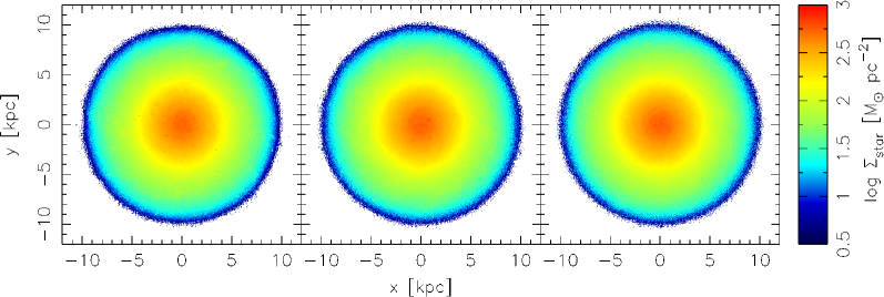
Figure 3: The stellar surface density at $t=1$, $2$, and $3~{}{\rm Gyr}$. For the stellar surface density, we use the sum of stellar particles formed from the gas particles and static surface density calculated by the Miyamoto-Nagai model (Miyamoto & Nagai, 1975).

Figure 4 shows the star-formation rate as a function of time. It is characterized by two phases: the initial rapidly increasing phase ($t<100~{}{\rm Myr}$), and the succeeding exponentially decreasing phase. The decay time-scale of the star-formation rate is $\sim 1~{}{\rm Gyr}$. This time scale is rather short compared to the estimation of the galactic chemical evolution (Larson, 1972; Yoshii et al., 1996), as our simulation does not consider the secular evolution due to gas accretion from the halo. This is also the reason why we stop our simulation at $t=3~{}{\rm Gyr}$, before the gas is exhausted. A model incorporating gas accretion will be used in our forthcoming papers.

Figure 4: Star-formation rate as a function of time.

3.1 AVR

Figure 5 shows the radial, azimuthal, vertical and total AVRs in our simulated galaxy at $t=2~{}\rm{Gyr}$. In this AVR analysis, we only use the star particles formed from gas. The red dots denote the results when only stars whose galactocentric distance $R$ was in the range $8~{}{\rm kpc}<R<9~{}{\rm kpc}$ were used, whereas the blue triangles represent the case where all regions were included. The velocity dispersions as a function of stellar age, $\tau$, are calculated by using the following equations:

$$\sigma_{\rm R}(\tau)=\left[\langle v_{R}^{2}\rangle_{\tau_{l}<\tau<\tau_{h}}-\langle v_{R}\rangle^{2}_{\tau_{l}<\tau<\tau_{h}}\right]^{1/2},$$ (5)

$$\sigma_{\rm\phi}(\tau)=\left[\langle(v_{\phi}-\overline{v_{\phi}}(R))^{2}\rangle_{\tau_{l}<\tau<\tau_{h}}-\langle v_{\phi}-\overline{v_{\phi}}(R)\rangle^{2}_{\tau_{l}<\tau<\tau_{h}}\right]^{1/2},$$ (6)

$$\sigma_{\rm z}(\tau)=\left[\langle v_{z}^{2}\rangle_{\tau_{l}<\tau<\tau_{h}}-\langle v_{z}\rangle^{2}_{\tau_{l}<\tau<\tau_{h}}\right]^{1/2},$$ (7)

$$\sigma_{\rm tot}(\tau)=\left[\sigma_{\rm R}(\tau)^{2}+\sigma_{\rm\phi}(\tau)^{2}+\sigma_{\rm z}(\tau)^{2}\right]^{1/2},$$ (8)

where $\tau_{l}$ and $\tau_{h}$ are the two edges of the age bin. $\langle v_{R}^{2}\rangle_{\tau_{l}<\tau<\tau_{h}}$ mean the average of stellar $v_{R}^{2}$ whose age is between $\tau_{l}$ and $\tau_{h}$. We apply the width of age bins in such a way that every bin has equal numbers of stars (2000 stars in each bin). For the distributions of velocity dispersions, the sampling range effect is insignificant.

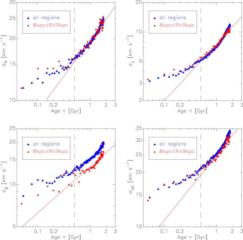
Figure 5: Radial (top left), vertical (top right), azimuthal (bottom left) and total (bottom right) AVRs in our simulated galaxy at $t=2~{}\rm{Gyr}$. The red dots indicate the AVR calculated with stellar particles found between $8~{}{\rm kpc}$ and $9~{}{\rm kpc}$ from the galactic center. The solid lines are the fitting results with a power-law function for the stellar particles in this region. For this procedure, we only use star particles older than $0.5~{}\rm{Gyr}$ (on the right side of the dashed line). The blue triangles indicate the AVR calculated with all stellar particles.

The solid lines in figure 5 represent the fitting results with a power-law function for stellar particles found between $R=8~{}{\rm kpc}$ and $9~{}{\rm kpc}$. Here, we adopt stars older than $0.5~{}{\rm Gyr}$. The functional forms of the fitted age-radial, azimuthal, vertical, and total velocity dispersion relations are

$$\sigma_{R}=19.4\left(\frac{\tau}{1~{}\rm{Gyr}}\right)^{0.37}~{}{\rm km~{}s^{-1}},$$ (9)

$$\sigma_{\phi}=13.4\left(\frac{\tau}{1~{}\rm{Gyr}}\right)^{0.33}~{}{\rm km~{}s^{-1}},$$ (10)

$$\sigma_{z}=7.36\left(\frac{\tau}{1~{}\rm{Gyr}}\right)^{0.59}~{}{\rm km~{}s^{-1}},$$ (11)

$$\sigma_{\rm tot}=25.0\left(\frac{\tau}{1~{}\rm{Gyr}}\right)^{0.36}~{}{\rm km~{}s^{-1}}.$$ (12)

The exponents of the radial, azimuthal, vertical, and total AVR and the ratio of the radial to vertical velocity dispersion are close to the observed values (see §1). The radial to vertical velocity dispersion ratio becomes

$$\frac{\sigma_{z}}{\sigma_{R}}=0.38\left(\frac{\tau}{1~{}\rm{Gyr}}\right)^{0.22}.$$ (13)

Observationally, the age dependence on this relation is not found. This weak dependence on $\tau$ in our simulated AVR again favors observations (Dehnen & Binney, 1998).

The blue triangles in figure 5 show the AVR calculated with all stellar samples. Here, we reapply the width of age bins in such a way that each bin has 10000 stars. Radial and vertical AVRs are similar to the local AVRs shown by the red points in spite of the difference in the samples. This agreement means that radial and vertical velocity dispersions are roughly constant throughout the disk region.

On the other hand, azimuthal velocity dispersion with all stellar samples is larger than those with local stars in the outer region ($8~{}{\rm kpc}<R<9~{}{\rm kpc}$). That is because the azimuthal velocity dispersion is determined by the epicycle approximation (Binney & Tremaine, 2008),

$$\frac{\sigma_{\rm\phi}^{2}}{\sigma_{\rm R}^{2}}=\frac{\kappa^{2}}{4\Omega^{2}},$$ (14)

where $\kappa$ and $\Omega$ are epicycle frequency and angular velocity, respectively, and the ratio of $\kappa$ and $\Omega$ changes depending on the galactocentric distance. Figure 6 shows $\sigma_{\rm\phi}^{2}/\sigma_{\rm R}^{2}$ and $\kappa^{2}/\Omega^{2}$ as a function of radius. There is a good agreement between then, which means that stellar motion is well described with the epicycle approximation. We see that $\sigma_{\rm\phi}^{2}/\sigma_{\rm R}^{2}\sim 0.5$ in the outer region ($R>8~{}{\rm kpc}$) where the rotational velocity becomes almost flat (as shown in figure 1), and this is also consistent with the prediction of the epicycle approximation. In the inner region ($R<8~{}{\rm kpc}$), however, the rotational velocity is an increasing function of R, and then $\sigma_{\rm\phi}^{2}/\sigma_{\rm R}^{2}$ are larger than those in the outer region. Here, $\sigma_{\rm R}$ does not depend on radius as mentioned in the above paragraph, and so, $\sigma_{\rm\phi}$ becomes a decreasing function of radius according to the epicycle approximation. Therefore, azimuthal AVR with all stellar samples deviates upward from that with local stars between $8~{}{\rm kpc}$ and $9~{}{\rm kpc}$ as shown in figure 5.

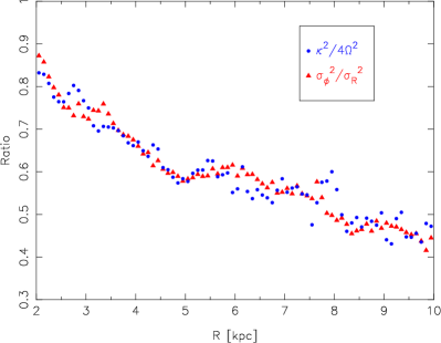
Figure 6: $\sigma_{\rm\phi}^{2}/\sigma_{\rm R}^{2}$ (red triangles) and $\kappa^{2}/4\Omega^{2}$ (blue dots) as a function of galactocentric radius at $t=2~{}{\rm Gyr}$. These two parameters are equal when epicycle approximation is satisfied.

Hereafter, we discuss the radial and vertical AVR with all stellar particles in the galactic disk to ensure sufficient samples and simplification.

It is worth noting that strong spiral arms do not develop in our simulated galaxies, although they are regarded as a heating source of radial velocity dispersion (Carlberg, 1987; Jenkins & Binney, 1990). Interestingly, without strong spiral arms, we can successfully reproduce the observed exponents of not only the vertical AVR, but also the radial one. We discuss this point in §4.

Figure 7 shows the AVRs at the three different epochs. We can see that the simulated AVRs of the three epochs do not overlap; there is a clear indication of the evolution of the AVR. Both the initial velocity dispersions and heating efficiency evolve. This is inconsistent with the conventional interpretation of the AVR, i.e., that it is the evolution track of stars on the age–velocity dispersion plane.

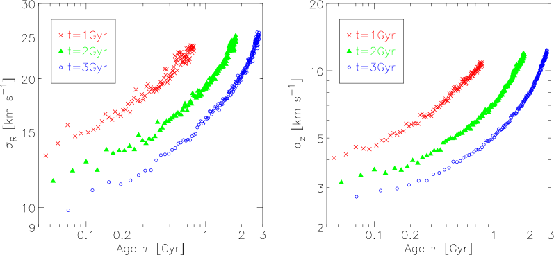
Figure 7: Evolution tracks of stellar age-velocity dispersions with different samples whose birth epoch is $t=1$, $2$, and $3~{}\rm{Gyr}$. Different symbols represent different groups.

In figure 8, we show the evolution tracks of stellar groups of 26 different epochs on the age–velocity dispersion planes. Each group has a different initial velocity dispersion and heating rate. The slope of each evolution sequence is less steep than those in observations. However, when we pick up values, for instance, at $t=2~{}{\rm Gyr}$ for all evolution sequences (black triangles in figure 8), we obtain AVRs that are consistent with those obtained from observations. This reveals that AVRs are inconsistent with the evolution tracks of stars on the age-velocity dispersion plane.

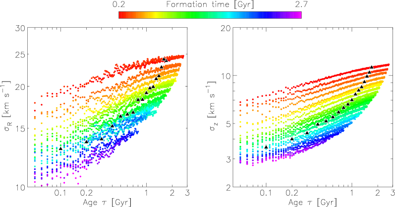
Figure 8: Dots show the time evolution of stellar velocity dispersion. The left and right panels show the radial and vertical velocity dispersion, respectively. Each color indicates a different birth time. The black triangle points show the AVR at $t=2$ Gyr.

3.2 Origins of simulated AVR

In the previous section, we showed that the AVR is not just a simple evolutionary track of stars on the age–velocity dispersion plane. In this section, we investigate two important factors that affect the evolution of stars on the age–velocity dispersion plane: the initial velocity dispersion (i.e. velocity dispersion at the birth time of stars) and the heating rate as a function of age. The evolution of the initial velocity dispersion is discussed in §3.2.1, while that of the heating rate is discussed in §3.2.2.

3.2.1 Zero-Age Velocity Dispersion

First, we discuss the stellar velocity dispersion at the birth time of stars. We call this the “zero-age velocity dispersion” (hereafter, ZAVD). As shown in figure 8, the ZAVD decreases with increasing age. This is one of the key reasons for the inconsistency between the AVR and the evolution tracks.

The ZAVD is strongly related to the velocity dispersion of the star-forming gas because it inherits the velocity dispersion. Figure 9 shows the radial and vertical velocity dispersions of gas that satisfy the star-formation criteria as a function of time. We can see that both velocity dispersions monotonically decrease with time and they can be fitted by a power-law function of $t$. However, their power-law indices are different; the index of the ZAVD for the vertical direction is about twice as steep as that for the radial direction. Gravitational interactions, radiative cooling, star formation and feedback play crucial roles in determining the ISM structure, and these effects depend on the mass of the gas in the disk. Therefore, it is natural that the status of the ISM is related to the origin of the AVR. In other words, the AVR involves the historical evolution of the ISM in a galaxy.

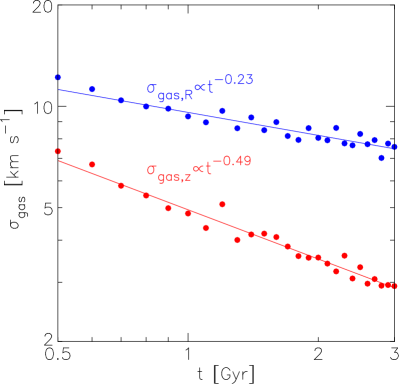
Figure 9: Velocity dispersion of gas that satisfies the star formation criteria as a function of time. Both the radial and vertical velocity dispersions are shown. Blue dots represent the radial-velocity dispersions, while red dots indicate the vertical-velocity dispersions. The lines are the results of the least square fitting with a power-law function.

3.2.2 Dynamical Heating Rate

In the previous section, we discussed the ZAVD. Here, we investigate the evolution of the dynamical heating rate (i.e. $d\sigma/dt$). Once these two factors are understood, we can use them to predict the entire evolution of the AVR.

Figure 10 shows the evolutions of vertical velocity dispersions, $\sigma_{\rm z}$, as a function of simulation time. Each sequence is characterized by two evolution phases: the rapidly increasing phase in the early stage and the asymptotically flattening phase in the late stage. Later time or higher velocity dispersion cause the heating rate to be lower.

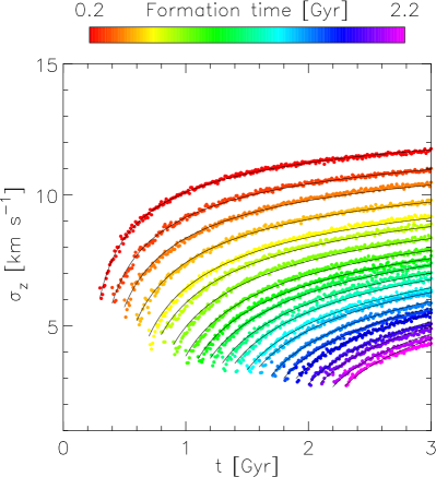
Figure 10: Vertical velocity dispersion as a function of time. Twenty-one groups have been selected. Each sequence represents the evolution of each group. Solid curves are results of the fitting (see Eq. (17)).

Figure 11 shows the vertical heating rate (${\rm d}\sigma_{z}/{\rm d}t$) as a function of $t$ and $\sigma_{\rm z}$. We chose four representative epochs and $\sigma_{z}$. Solid lines are the fitting result with power-law functions of $\sigma_{z}$ and $t$. We can see that the heating rate obtained by our simulation is well fitted by power-law functions.

Using the fitting results shown in figure 11, we can describe the heating rate as a function of $t$ and $\sigma_{z}$:

$$\frac{d\sigma_{z}}{dt}\propto t^{-\alpha}\sigma_{z}^{-\beta}.$$ (15)

We apply this equation to sequences in figure 10 and then we obtain the concrete values of $\alpha$ and $\beta$. With these values, we have

$$\frac{d\sigma_{z}}{dt}\propto t^{-1.3}\sigma_{z}^{-1.5}.$$ (16)

By integrating this equation, we finally have

$$\sigma_{z}=11.8\left[A-\left(\frac{t}{1~{}{\rm Gyr}}\right)^{-0.33}\right]^{0.40}~{}{\rm km~{}s^{-1}},$$ (17)

where $A$ is a constant of an integral. The different sequence found in figure 10 can be expressed by choosing a different value of $A$.

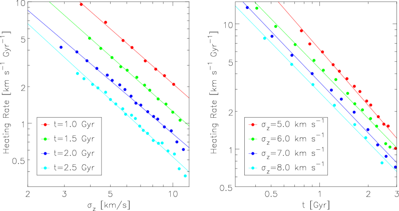
Figure 11: Heating rates as a function of $\sigma_{z}$ (left) and as a function of time $t$. Four representative epochs ($t=1.0$, $1.5$, $2.0$ and $2.5~{}\rm{Gyr}$) and four representative values of $\sigma_{z}$ ($\sigma_{z}=5.0$, $6.0$, $7.0$ and $8.0~{}{\rm km~{}s^{-1}}$) are employed. The solid lines represent the results of fitting with power-law functions.

In figure 2, the dense gas ($n_{\rm H}>100~{}{\rm cm^{-3}}$) has clumpy structures, and is expected to play the role of a heating source. This clumpy and dense gas is decreasing with simulation time. We suspect that the decreasing heating rate with increasing simulation time may result from the decrease in the dense gas. Hence, we show the time evolution of the dense gas mass $M_{\rm dens}$ in figure 12. Here, we define the gas above the star formation threshold as the dense gas. We see that the mass of the dense gas monotonically decreases and it can be fitted by a simple power-law function with the power-law index of $-1.24$. Interestingly, the power-law index is consistent with that for the simulation time found in Eq. (16). This implies that the time evolution of the heating rate in our simulation is controlled by the total mass of the dense gas.

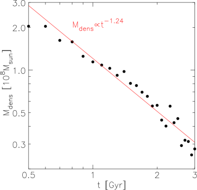
Figure 12: Time evolution of gas mass that is much denser than the star formation threshold density. The solid line indicates the result of the fitting by a power-law function and its exponent is $-1.24$.

Our result can be reduced to that obtained in the previous study where the contribution of gas is unchanged (Spitzer & Schwarzschild, 1951, 1953; Kokubo & Ida, 1992; Hänninen & Flynn, 2002). Consider the case in which the dense gas mass does not evolve; this can be described by letting $\alpha=0$ in Eq. (15), and then we obtain

$$\sigma_{z}\propto\left(A-t\right)^{1/(\beta+1)}.$$ (18)

This is consistent with the time evolution of velocity dispersion shown by a previous work (e.g. Hänninen & Flynn (2002)), where the models treated the GMCs as a time-independent potential.

4 Discussion and Summary

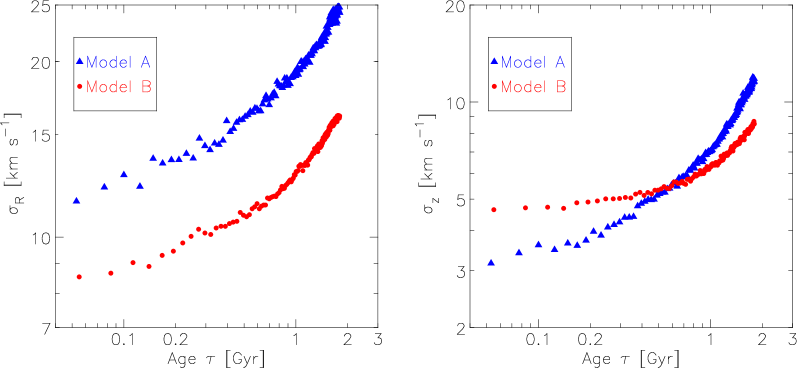
Figure 13: Radial and vertical AVR of two simulations. Blue and red points show the AVR of Models A and B, respectively.

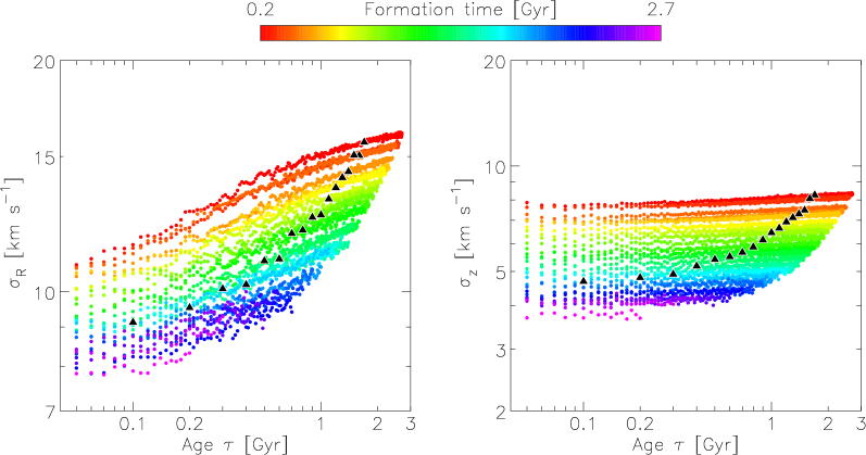
Figure 14: Same as Figure 8, but about a Model B whose gravitational softening length and star formation density threshold are $100\rm{pc}$ and $1\rm{cm^{-3}}$ respectively.

Our simulation shows that the AVR is not the evolution track of stars on the age–velocity dispersion plane. This result means that the AVR can be reproduced even if the heating rate is smaller than the slope of the AVR. The time evolution of the stellar velocity dispersion depends upon the combination of the initial velocity dispersion and the heating rate. In particular, the AVR is strongly affected by the evolution of the ZAVD.

The importance of the ZAVD was pointed out by Wielen (1977); however they did not attempt to elucidate the details because of the complicated nature of gas dynamics. Recent numerical simulations of galaxy formation also demonstrate that the ZAVD has a crucial role in the establishment of the AVR (Bird et al., 2013; Grand et al., 2016). The observations of turbulent gas disk at high redshift (Förster Schreiber et al., 2009) support the presence of the evolution of ZAVD.

The other key process for establishing the AVR is the secular heating due to dense gas. This is consistent with Aumer et al. (2016a), who shows that the evolution of heating history shapes an AVR. Our simulation can successfully derive the contribution of this process. We point out that the sufficient spatial resolution and realistic star-formation thresholds are crucial to describe the evolution of the AVR via dense gas scattering.

Table 2: Parameters of simulation models.

Models	$\epsilon$ 1 [pc]	$n_{\rm th}$ 2 [${\rm cm^{-3}}$]	$N_{\rm ini}$ 3
Model A	10	100	$10^{6}$
Model B	100	1	$10^{6}$

• Softening length

• Star formation density threshold

• Initial particles

Figure 13 shows the radial and vertical AVRs of two simulations: one is obtained by our simulations with the fiducial parameters (Model A) and the other employs the larger gravitational softening length ($100~{}{\rm pc}$) and lower star-formation thresholds ($1~{}{\rm cm^{-3}}$) that are widely used in cosmological simulations of galaxy formation (Model B). Table 2 shows parameters of the two models. It is apparent that the AVRs with the low thresholds are quite different from those obtained by our fiducial model; for instance, the ZAVDs for both radial and vertical directions are different. The low threshold density for star formation decreases the radial ZAVD while it increases the vertical ZAVD. The former is due to the lack of high-density structures, and the latter is due to the relatively thick star-forming region in the gas disk (see Saitoh et al. (2008)). Interestingly, the heating rate in the radial direction is almost identical to that of the reference simulation while that in the vertical direction is quite different from that of the reference simulation. The reason for the discrepancy in the vertical direction is the larger ZAVD.

Figure 14 shows the evolution tracks of different groups for the low-resolution model. In particular, the evolution tracks of the vertical direction are quite different from those in the reference model (see figure 8). The adoption of star-formation thresholds, which are justified by high mass resolution, is critical to any discussion of the formation and evolution of the AVR. We will show the results of the systematic survey of the numerical effects on the AVR in a forthcoming paper.

So far, we have worked with a very simplified model; for instance, there is no gas accretion, and the fixed halo and stellar potentials are used. We need to improve our model and make it more realistic so that we can discuss the long-time evolution of the AVR in more detail and can measure the contribution of spiral arms and the bar. The contribution of the spiral arms to the AVR may turn out to be limited. Previous studies have suggested that transient, recurrent (so-called ‘dynamic’) spiral arms lead to radial migration and it does not increase the radial velocity dispersion significantly (Sellwood & Binney, 2002; Grand et al., 2012b, a; Roškar et al., 2012; Baba et al., 2013).

As a next step, we will introduce the effects of gas accretion to our model. By investigating the relation between the accretion history and the AVR, it might be possible to impose constraints on the Milky Way-like galaxy formation.

The GAIA era is approaching. The GAIA will provide information about the proper motions of about one billion stars (Perryman et al., 2001). By combining it with other observations, such as the RAVE (Steinmetz et al., 2006), APOGEE (Majewski et al., 2016), SEGUE (Yanny et al., 2009), and Gaia-ESO survey (Gilmore et al., 2012), we will be able to depict the fine structure of the Milky Way galaxy. Our model can be tested by the results of this new generation of observations.

We thank the referee for his/her constructive comments which helped improve the manuscript. Numerical computations in this paper were performed on Cray XC30 at the Center for Computational Astrophysics, National Astronomical Observatory of Japan. TRS is supported by a Grant-in-Aid for Scientific Research (26707007) of Japan Society for the Promotion of Science. JB was supported by HPCI Strategic Program Field 5 ‘The origin of matter and the universe’ and JSPS Grant-in-Aid for Young Scientists (B) Grant Number 26800099.

References

- Aumer et al. (2016a) Aumer, M., Binney, J., & Schönrich, R. 2016a, MNRAS, 462, 1697
- Aumer et al. (2016b) —. 2016b, MNRAS, 459, 3326
- Aumer & Binney (2009) Aumer, M., & Binney, J. J. 2009, MNRAS, 397, 1286
- Baba et al. (2017) Baba, J., Morokuma-Matsui, K., & Saitoh, T. R. 2017, MNRAS, 464, 246
- Baba et al. (2013) Baba, J., Saitoh, T. R., & Wada, K. 2013, ApJ, 763, 46
- Balsara (1995) Balsara, D. S. 1995, Journal of Computational Physics, 121, 357
- Bate & Burkert (1997) Bate, M. R., & Burkert, A. 1997, MNRAS, 288, 1060
- Binney & Tremaine (2008) Binney, J., & Tremaine, S. 2008, Galactic Dynamics: Second Edition (Princeton University Press)
- Bird et al. (2013) Bird, J. C., Kazantzidis, S., Weinberg, D. H., et al. 2013, ApJ, 773, 43
- Bland-Hawthorn & Gerhard (2016) Bland-Hawthorn, J., & Gerhard, O. 2016, ARA&A, 54, 529
- Brook et al. (2012) Brook, C. B., Stinson, G. S., Gibson, B. K., et al. 2012, MNRAS, 426, 690
- Carlberg (1987) Carlberg, R. G. 1987, ApJ, 322, 59
- Carlberg & Sellwood (1985) Carlberg, R. G., & Sellwood, J. A. 1985, ApJ, 292, 79
- De Simone et al. (2004) De Simone, R., Wu, X., & Tremaine, S. 2004, MNRAS, 350, 627
- Dehnen & Binney (1998) Dehnen, W., & Binney, J. J. 1998, MNRAS, 298, 387
- Förster Schreiber et al. (2009) Förster Schreiber, N. M., Genzel, R., Bouché, N., et al. 2009, ApJ, 706, 1364
- Freeman & Bland-Hawthorn (2002) Freeman, K., & Bland-Hawthorn, J. 2002, ARA&A, 40, 487
- Gilmore et al. (2012) Gilmore, G., Randich, S., Asplund, M., et al. 2012, The Messenger, 147, 25
- Gingold & Monaghan (1977) Gingold, R. A., & Monaghan, J. J. 1977, MNRAS, 181, 375
- Grand et al. (2012a) Grand, R. J. J., Kawata, D., & Cropper, M. 2012a, MNRAS, 426, 167
- Grand et al. (2012b) —. 2012b, MNRAS, 421, 1529
- Grand et al. (2016) Grand, R. J. J., Springel, V., Gómez, F. A., et al. 2016, MNRAS, 459, 199
- Hänninen & Flynn (2002) Hänninen, J., & Flynn, C. 2002, MNRAS, 337, 731
- Holmberg et al. (2007) Holmberg, J., Nordström, B., & Andersen, J. 2007, A&A, 475, 519
- Holmberg et al. (2009) —. 2009, A&A, 501, 941
- House et al. (2011) House, E. L., Brook, C. B., Gibson, B. K., et al. 2011, MNRAS, 415, 2652
- Huang & Carlberg (1997) Huang, S., & Carlberg, R. G. 1997, ApJ, 480, 503
- Hubber et al. (2006) Hubber, D. A., Goodwin, S. P., & Whitworth, A. P. 2006, A&A, 450, 881
- Jenkins & Binney (1990) Jenkins, A., & Binney, J. 1990, MNRAS, 245, 305
- Just & Jahreiß (2010) Just, A., & Jahreiß, H. 2010, MNRAS, 402, 461
- Katz (1992) Katz, N. 1992, ApJ, 391, 502
- Kokubo & Ida (1992) Kokubo, E., & Ida, S. 1992, PASJ, 44, 601
- Kumamoto & Noguchi (2016) Kumamoto, J., & Noguchi, M. 2016, ApJ, 822, 110
- Lacey & Ostriker (1985) Lacey, C. G., & Ostriker, J. P. 1985, ApJ, 299, 633
- Larson (1972) Larson, R. B. 1972, Nature Physical Science, 236, 7
- Lucy (1977) Lucy, L. B. 1977, AJ, 82, 1013
- Majewski et al. (2016) Majewski, S. R., APOGEE Team, & APOGEE-2 Team. 2016, Astronomische Nachrichten, 337, 863
- Makino (1991) Makino, J. 1991, PASJ, 43, 859
- Martig et al. (2014) Martig, M., Minchev, I., & Flynn, C. 2014, MNRAS, 443, 2452
- Miyamoto & Nagai (1975) Miyamoto, M., & Nagai, R. 1975, PASJ, 27, 533
- Monaghan (1992) Monaghan, J. J. 1992, ARA&A, 30, 543
- Monaghan (1997) —. 1997, Journal of Computational Physics, 136, 298
- Nakanishi & Sofue (2006) Nakanishi, H., & Sofue, Y. 2006, PASJ, 58, 847
- Navarro et al. (1997) Navarro, J. F., Frenk, C. S., & White, S. D. M. 1997, ApJ, 490, 493
- Nordström et al. (2004) Nordström, B., Mayor, M., Andersen, J., et al. 2004, A&A, 418, 989
- Okamoto et al. (2008) Okamoto, T., Nemmen, R. S., & Bower, R. G. 2008, MNRAS, 385, 161
- Perryman et al. (2001) Perryman, M. A. C., de Boer, K. S., Gilmore, G., et al. 2001, A&A, 369, 339
- Robertson & Kravtsov (2008) Robertson, B. E., & Kravtsov, A. V. 2008, ApJ, 680, 1083
- Roškar et al. (2012) Roškar, R., Debattista, V. P., Quinn, T. R., & Wadsley, J. 2012, MNRAS, 426, 2089
- Saitoh et al. (2008) Saitoh, T. R., Daisaka, H., Kokubo, E., et al. 2008, PASJ, 60, 667
- Saitoh et al. (2006) Saitoh, T. R., Koda, J., Okamoto, T., Wada, K., & Habe, A. 2006, ApJ, 640, 22
- Saitoh & Makino (2009) Saitoh, T. R., & Makino, J. 2009, ApJ, 697, L99
- Saitoh & Makino (2010) —. 2010, PASJ, 62, 301
- Saitoh & Makino (2016) —. 2016, ApJ, 823, 144
- Salpeter (1955) Salpeter, E. E. 1955, ApJ, 121, 161
- Seabroke & Gilmore (2007) Seabroke, G. M., & Gilmore, G. 2007, MNRAS, 380, 1348
- Sellwood & Binney (2002) Sellwood, J. A., & Binney, J. J. 2002, MNRAS, 336, 785
- Sharma et al. (2014) Sharma, S., Bland-Hawthorn, J., Binney, J., et al. 2014, ApJ, 793, 51