Dynamical universality classes of simple growth and lattice gas models

Abstract

Large scale, dynamical simulations have been performed for the two dimensional octahedron model, describing the Kardar–Parisi–Zhang (KPZ) for nonlinear, or the Edwards–Wilkinson (EW) class for linear surface growth. The autocorrelation functions of the heights and the dimer lattice gas variables are determined with high precision. Parallel random-sequential (RS) and two-sub-lattice stochastic dynamics (SCA) have been compared. The latter causes a constant correlation in the long time limit, but after subtracting it one can find the same height functions as in case of RS. On the other hand the ordered update alters the dynamics of the lattice gas variables, by increasing (decreasing) the memory effects for nonlinear (linear) models with respect to RS. Additionally, we support the KPZ ansatz and the Kallabis–Krug conjecture in $2+1$ dimensions and provide a precise growth exponent value $\beta=\num{0.2414}(2)$. We show the emergence of finite size corrections, which occur long before the steady state roughness is reached.

Keywords: driven lattice gas, surface growth, autocorrelation, Kardar–Parisi–Zhang class, stochastic cellular automaton, Edwards–Wilkinson class

1 Introduction

Nonequilibrium systems are known to exhibit dynamical scaling, when the correlation length diverges as $\xi\propto t^{1/z}$, characterized by the exponent $z$. Simplest models are driven lattice gases (DLG) [1], which in certain cases can be mapped onto surface growth [2, 3]. Therefore, understanding DLGs, which is far from being trivial due to the broken time reversal symmetry [4], and is possible mostly by numerical simulations only, sheds some light on the corresponding interface phenomena [5]. The simplest example is the asymmetric simple exclusion process (ASEP) of particles [6], in which particles and holes can be mapped onto binary surface slopes [7, 8] and the corresponding continuum model can be described by the Kardar–Parisi–Zhang (KPZ) equation [9]

$$\partial_{t}h(\mathbf{r},t)=\sigma\nabla^{2}h(\mathbf{r},t)+\lambda(\nabla h(\mathbf{r},t))^{2}+\eta(\mathbf{r},t)\ ,$$ (1)

where the scalar field $h(\mathbf{r},t)$ is the height, progressing in the $D$ dimensional space relative to its mean position, that moves linearly with time $t$. This equation was inspired in part by the stochastic Burgers equation [10] and can describe the dynamics of simple growth processes in the thermodynamic limit [11], randomly stirred fluids [12], directed polymers in random media [13], dissipative transport [14, 15], and the magnetic flux lines in superconductors [16]. In case of surface growth $\sigma$ represents a surface tension, competing with the nonlinear up–down anisotropy of strength $\lambda$ and a zero mean valued Gaussian white noise $\eta$. This field exhibits the covariance $\langle\eta(\mathbf{r},t)\eta(\mathbf{x^{\prime}},t^{\prime})\rangle=2\Gamma\delta^{D}(\mathbf{r-r^{\prime}})(t-t^{\prime})$. The $\lambda=0$, linear equation describes the Edwards–Wilkinson (EW) [17] surface growth, an exactly solvable equilibrium system.

Several discrete models obeying these equations have been studied [7, 18, 2]. The morphology of a surface of linear size $L$ is usually described by the squared interface width

$$W^{2}(L,t)=\frac{1}{L^{2}}\,\sum_{i,j}^{L}\,h^{2}_{i,j}(t)-\Bigl{(}\frac{1}{L}\,\sum_{i,j}^{L}\,h_{i,j}(t)\Bigr{)}^{2}\ .$$ (2)

In the absence of any characteristic length simple growth processes are expected to be scale-invariant [19]

$$W(L,t)\propto L^{\alpha}f(t/L^{z})\ ,$$ (3)

with the universal scaling function $f(u)$:

$$f(u)\propto\left\{\begin{array}[]{lcl}u^{\beta}&{\rm if}&u\ll 1\\ {\rm const.}&{\rm if}&u\gg 1\end{array}\right.$$ (4)

Here $\alpha$ is the roughness exponent in the stationary regime, when the correlation length $\xi$ has grown to exceeded $L$, and $\beta$ is the growth exponent, describing the intermediate time behavior. The dynamical exponent $z$ can be expressed as the ratio of the growth exponents:

$$z=\alpha/\beta\$$ (5)

Apart from the exponents, the shapes of the rescaled width and height distributions of the interfaces $\Psi_{L}(\varphi_{L})$ were shown to be universal in KPZ models in both the steady state [20] and the growth regime [21]. Here, $\varphi_{L}$ denotes the interface observable in question, $W^{2}$ or $h$, in a system of linear size $L$. In fact many people define the universality classes by these quantities, which can be obtained exactly in one dimension for various surface geometries, like flat [22] or curved [23, 24, 22] interfaces. The non-rescaled probability distributions are denoted by $P_{L}(\varphi_{L})$ and their moments are defined via the distribution averages as:

$$\Phi^{n}_{L}[\varphi_{L}] =\int\limits_{0}^{\infty}\left(\varphi_{L}-\langle\varphi_{L}\rangle\right)^{n}P_{L}(\varphi_{L})\,\mathrm{d}\varphi_{L}\quad,$$ (6)

Two standard measures of the shape, the skewness

$$S_{L}[\varphi_{L}] =\langle\Phi^{3}_{L}[\varphi_{L}]\rangle/\langle\Phi^{2}_{L}[\varphi_{L}]\rangle^{3/2}$$ (7)

and the kurtosis

$$Q_{L}[\varphi_{L}] =\langle\Phi^{4}_{L}[\varphi_{L}]\rangle/\langle\Phi^{2}_{L}[\varphi_{L}]\rangle^{2}-3\quad,$$ (8)

are calculated in the steady state or in the growth regime. The universal, rescaled forms are:

$$\Psi_{L}[W^{2}(L)] =\langle W^{2}(L)\rangle P_{L}(W^{2}(L)/\langle W^{2}(L)\rangle)$$ (9)

for the width and

$$\Psi_{L}[h_{L}(\mathbf{r})] =L^{\alpha}P_{L}(h_{L}(\mathbf{r})/L^{\alpha})$$ (10)

for the surface height. Note, that $\left\langle h_{L}\right\rangle\equiv\Phi_{L}^{0}[h_{L}]\equiv 0$ in the co-moving frame of the surface.

While many systems are described by a single dynamical length scale, aging ones are best characterized by two-time quantities, such as the dynamical correlation and response functions [25]. In the aging regime: $s\gg\tau_{\rm m}$ and $t-s\gg\tau_{\rm m}$, where $\tau_{\rm m}$ is a microscopic time scale and $s$ is the start time, when the snapshot is taken, one expects the following law for the autocorrelation function

$$C(t,s) =\left\langle\phi(t,\mathbf{r})\phi(s,\mathbf{r})\right\rangle-\left\langle\phi(t,\mathbf{r})\right\rangle\left\langle\phi(s,\mathbf{r})\right\rangle$$ (11)

$$\propto s^{-b}(t/s)^{-\lambda_{C}/z}\quad,$$ (12)

here $\langle\rangle$ denotes averaging over both lattice sites and independent samples; $\lambda_{C}$ is the autocorrelation and $b$ is the aging exponent. The function $\phi$ denotes the measured quantity, which can be the particle density of the lattice gas or the surface height $h(t,\mathbf{r})$. In the latter case,

$$C_{h}(t,s) =\left\langle h(t,\mathbf{r})h(s,\mathbf{r})\right\rangle-\left\langle h(t,\mathbf{r})\right\rangle\left\langle h(s,\mathbf{r})\right\rangle\ ,$$ (13)

for $$t=s$$ one finds:

$$=\left\langle h^{2}(s,\mathbf{r})\right\rangle-\left\langle h(s,\mathbf{r})\right\rangle^{2}=W^{2}(L\to\infty,s)\propto s^{-b_{h}}\cdot f_{C}(1)~{}.$$

This implies the relation

$$b_{h}=-2\beta~{},$$ (14)

which must be satisfied in the $L\to\infty$ and $s\to\infty$ limit. We have also calculated the auto-correlation of the slope (lattice gas occupancy variables) $n(t,\mathbf{r})$ as:

$$C_{s}(t,s) =\left\langle\left(n(t,\mathbf{r})-\overline{n}\right)\left(n(s,\mathbf{r})-\overline{n}\right)\right\rangle$$

$$=\left\langle n(t,\mathbf{r})n(s,\mathbf{r})\right\rangle-\overline{n}^{2}$$

$$=s^{-b_{s}}f^{\prime}_{C}\left(\frac{t}{s}\right),$$ (15)

where $\overline{n}=\num{0.5}$ is the conserved average occupancy of sites. However, $C_{s}(t,s)$ decays much faster than the height auto-correlator and obtaining reasonable signal/noise ratio requires much higher statistics.

A dynamic, perturbative renormaliztion group (RG) analysis of the KPZ equation [26, 27] suggested that the short and the long time scaling behavior of the height correlation function are identical and deduced a scaling relation for the exponent of $C_{h}(t\gg s,s\to 0)\propto(t/s)^{-\theta}$ as:

$$\theta=(D+4)/z-2\ .$$ (16)

Since $\theta=\lambda_{C}/z+2\beta$, due to (14) the relation (16) holds exactly in the solvable $1+1$ dimensional case. In $D\geq 2$ dimensions perturbative RG can’t access the strong coupling KPZ fixed point [28], thus the validity of this law should be tested by precise exponent estimates.

A conjecture based on a purely geometric argument, advanced by Kallabis and Krug [29], which can also be deduced from the scaling relation (16) claims $D=\lambda_{C}$ in any dimensions. In [30] we provided marginal agreement for this in $D=2$ and Ref. [31] also suggested it using solid-on-solid models, although clear power laws were not reached within the times studied. Here we provide stronger numerical evidence in case of different lattice gas dynamics.

In aging systems a similar scaling form is expected for the autoresponse function of the field $\phi$:

$$R(t,s)=\left.\frac{\delta\left\langle\phi(t)\right\rangle}{\delta j(s)}\right|_{j=0}=s^{-1-a}f_{R}\left(\frac{t}{s}\right)\,$$ (17)

where $j$ is the external conjugate to $\phi$ and $a$ denotes the so-called aging exponent $a$. The universal scaling function exhibits the asymptotic behavior $f_{R}(t/s)\sim(t/s)^{-\lambda_{R}/z}$ with the autoresponse exponent $\lambda_{R}$. In equilibrium $\lambda_{C}=\lambda_{R}$ and $a=b$ due to the fluctuation-dissipation (FD) symmetry [32]. In nonequilibrium systems these exponents can be completely independent. Therefore, we shall determine them one-by-one and investigate if some extended FD relation may occur among them. This has been done, using our very recent aging response exponents [33], determined to test the validity of a logarithmic extension of local scale-invariance (LSI) [32] proposed in [34] and work on such extensions in other models has been continued recently [35, 36].

Throughout the present study we compare results obtained using two common updating schemes for lattice models: random-sequential (RS) and stochastic cellular automaton (SCA) (checkerboard) updates. We find constant as well as non-trivial corrections to the dynamical correlation functions produced by the SCA and also observe differences in the corrections to scaling.

This paper is structured as follows. The investigated model and the simulation algorithms are introduced in Sect. 2. Roughness growth results are presented in Sect. 3.1, while autocorrelation and aging date can be found in Sect. 3.2. We conclude the paper with a discussion of the main implications of our results in Sect. 4.

2 Models and simulation algorithms

Discrete models set up for KPZ have been studied a lot in the past decades [7, 18, 2]. A mapping between KPZ surface growth in two dimensions and driven lattice gases has been advanced in [37, 38] an extension of the "rooftop" model of [7, 8]. We called it octahedron model, characterized by binary slope variables $\sigma_{x/y}$ at the edges connecting top vertexes of octahedra [38] representing atoms. The $\sigma_{x/y}$ take the values $0$ or $1$ to encode down or up slopes, respectively. Thus deposition or removal of octahedra corresponds to a stochastic cellular automaton, with the simple Kawasaki update rules [38]

$$\left(\begin{array}[]{cc}0&1\\ 0&1\end{array}\right)\overset{p}{\underset{q}{\rightleftharpoons}}\left(\begin{array}[]{cc}1&0\\ 1&0\end{array}\right)\quad,$$ (18)

where $p$ and $q$ denote the acceptance probabilities. Projecting the edges onto a plane yields a square lattice of slopes, which can then be considered as occupancy variables. This maps the octahedron model onto self-reconstructing dimers following an oriented migration along the bisection of the $x$ and $y$ directions of the surface (see figure 1 or figure 11 of the supplemental material for a 3D depiction). In this picture the surface heights must be defined relative to a reference point $h_{1,1}=0$ and can be reconstructed from the slope variables as

$$h_{i,j}=\sum_{l=1}^{i}[2\sigma_{x}(l,1)-1]+\sum_{k=1}^{j}[2\sigma_{y}(i,k)-1]\ .$$ (19)

Discrete surface and DLG models usually apply random sequential dynamics. On the other hand in certain cases synchronous, so called SCA-like site updating can prove to be useful, especially for simulations on parallel computers. This study is based on massively parallel simulations on graphics cards (GPUs). Synchronous updating in case of one-dimensional ASEP models has already been investigated [39, 40, 41]. One-point quantities in the bulk, like particle current or surface growth have been shown to exhibit the same behavior as in case of RS. However, n-point correlation functions may be different.

Here we extend the parallel two-sublattice scheme developed for ASEP [40] to the two dimensional dimer model as shown on figure 1, and compare the dynamical scaling results with those of the RS dynamics.

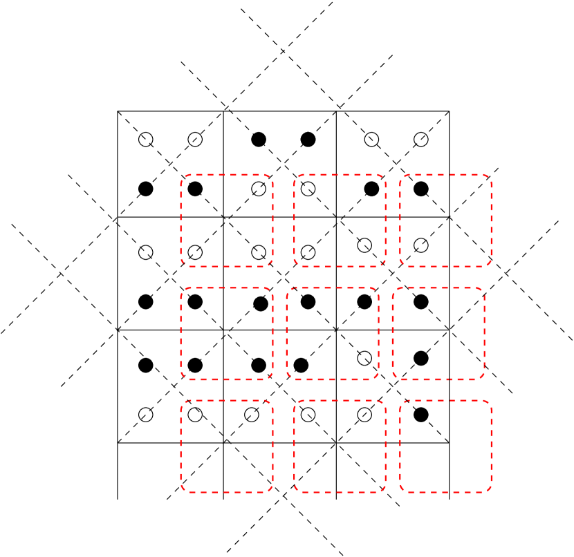
Figure 1: Schematics of the two sub-lattice SCA updates of the dimer lattice gas model. Circles: empty sites (down slopes), bullets: filled sites (up slopes). Solid, black lines denote areas, where the rule (18) is applied at $t$ odd, while dashed red lines encircle areas for update at even $t$ time steps. Diagonal, dashed lines are parallel with the $x$ and $y$ axis and are projection of the octahedron edges.

While the latter produces uncorrelated deposition and removal processes, SCA dynamics attempts updates in a checkerboard pattern, which are thusly correlated. Because of this, blocks of sites to be updated can be visited in a sequential order within a SCA sub-lattice step, allowing for very efficient implementation [42], matching perfectly parallel processors of GPU architectures [43].

Performing RS simulations on GPUs is less straight-forward, because unwanted correlations may be introduced [30]. In order to eliminate these and to achieve results as close to really sequential simulations as possible, we apply a new DD scheme, with two layers of DD to match the GPU architecture. At level one, in a double tiling decomposition, the origin is moved randomly after each sweep of the lattice (DTr). At level two, these tiles are subdivided further, with a logical dead border (DB) scheme. Collective update attempts are preformed inside these cells, excluding one lattice site-wide borders around each. Here, the decomposition origin is moved randomly after each collective update attempt. This scheme will be referred to as DTrDB in the following. Details of the new implementation are documented elsewhere [44].

In order to estimate the asymptotic values of different exponents for $t\to\infty$, local slope analyses of the scaling laws were performed [5]. For example in case of the interface width growth we used

$$\beta_{\mathrm{eff}}\left(\frac{t_{i}-t_{i/2}}{2}\right)=\frac{\ln W(L\to\infty,t_{i})-\ln W(L\to\infty,t_{i/2})}{\ln(t_{i})-\ln(t_{i/2})}\,.$$ (20)

In our studies the simulation time, measured in Monte Carlo steps (MCS), between two measurements was increased exponentially

$$t_{i+1}=(t_{i}+10)\mathrm{e}^{m}\quad,$$ (21)

using $m=\num{.01}$ and $t_{0}=0$. A flat initial state is realized by a zig-zag pattern with $W^{2}(L,t_{0})=\num{.25}$. The simulations are subject to periodic boundary conditions.

Statistical uncertainties are provided as $1\sigma$–standard errors, defined as $\Delta_{1\sigma}x=\sqrt{\langle x^{2}\rangle-\langle x\rangle^{2}/(N-1)}$. Throughout this study we used the implementation of the Levenberg–Marquadt algorithm [45, 46] in the gnuplot software [47] for non-linear least squares fitting.

For $p=q>0$ the octahedron model describes the surface growth of the EW equation [38] in $2+1$ dimensions. In this case the autocorrelation function of heights has been derived [48, 49]:

$$C_{\mathrm{h}}^{\mathrm{EW}}=c_{0}\ln\left(\frac{t+s}{t-s}\right)\quad,$$ (22)

where $c_{0}$ is a model-dependent constant. This function approaches $0$ for $t\gg s$ as a power law (PL) with the exponent $\lambda_{C,\text{h,\lx@glossaries@gls@link{acronym}{ew}{\leavevmode EW}}}/z_{\text{\lx@glossaries@gls@link{acronym}{ew}{\leavevmode EW}}}=1$, where $z_{\text{\lx@glossaries@gls@link{acronym}{ew}{\leavevmode EW}}}=2$. In Sect. 3.2.2 we shall reproduce this result numerically as a test of our simulations.

3 Results

Extensive dynamical simulations were performed using both RS and SCA updating schemes. To avoid finite-size effects we considered large systems with lateral sizes of $L=2^{16}$.

In SCA simulations the deposition probability must be $p<1$ in order to allow stochastic noise. We investigated three cases: $p=\num{.5},\num{.75}$ and $\num{.95}$ in depth. While KPZ runs were performed without removals: $q=0$, in the EW growth we applied $p=q=1$ for RS and $p=q=\num{.5}$ for SCA.

The roughness scaling of the interface width is analyzed in section 3.1. This is followed by autocorrelation and aging studies of the height as well as lattice-gas variables in section 3.2.

3.1 Roughness scaling

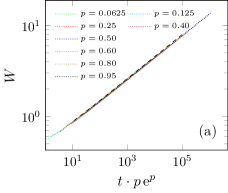
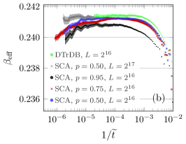
Figure 2: Width-scaling under SCA dynamics. (a) Width curves collapsed over $p$ by rescaling time as $\widetilde{t}=t\cdot p\,\mathrm{e}^{p}$. For comparison the DTrDB result is also shown (black dashed line). (b) Effective scaling exponents under SCA dynamics for $p=\num{.95}$ ($n\geq 2254$), $p=\num{.75}$ ($n\geq 6430$) and $p=\num{.5}$ ($n\geq 373$, $n\geq 3062$). RS data is shown for comparison ($n\geq 708$). Propagated $1\sigma$ error bars are attached to the effective exponents, merging into an error-corridor at late times due to the dense placing of points.

To compare numerical results coming from different updates we determined experimentally a scaling function $f(t,p)$, that provides collapses of $W(L,f(t,p))$ for different dynamics. In case or RS dynamics this function is linear $f_{\mathrm{RS}}(t,p)\propto p$. Since the $p\to 0$ limit of the SCA corresponds to RS updating, we tried to extend the linear form analytically. A smaller survey study of SCA for a larger number of different $p\leq\num{.95}$ values was used to obtain this function numerically and resulted in the following nonlinear extension:

$$f_{\mathrm{SCA}}(t,p)=\widetilde{t}(p)=t\cdot p\,\mathrm{e}^{p}\ .$$ (23)

The speedup with respect to linear function of RS can be understood as follows. A dimer, that was moved at a given time step becomes the target of another update at the next sub-lattice step in the $p\to 1$, $q=0$ case. This is more effective than random sequential updating. Therefore, the roughness growth is faster under SCA than under RS dynamics. One can test this function by observing a reasonably collapse on figure 2(a) for different $p$-s of SCA as compared to the RS results.

Figure 2(b) shows the effective scaling exponents $\beta_{\mathrm{eff}}$, as defined in $\eqref{eq:beff}$, for SCA and RS simulations as the function of the rescaled time variable. Most notably, the $\beta_{\mathrm{eff}}$ exponent results exhibit slightly shifted plateaus for almost two decades in time, but the difference lies well within the error-margin of our best published result $\beta_{\mathrm{eff}}=\num{.2415}(15)$ [50].

Random-sequential

The pronounced plateau visible for DTrDB, suggests that corrections at these late times are small, thus the $\beta_{\mathrm{eff}}$ here should be close to the asymptotic value for $\beta$. This leads to the estimate $\beta=\num{.2414}(2)$, where the error margin is about the size of the $1\sigma$-error bars attached to the effective exponents at late times.

Stochastic cellular automaton

Like in the RS case, there are almost two decades long plateaus in the effective exponents, depending on $p$ for $L=2^{16}$. The plateau value differences are beyond the statistical fluctuations and the DTrDB result. The deviation from the RS result shrinks as we decrease $p$, i.e. as we introduce more and more randomness. This is plausible, but smaller $p$ also means less effective simulations.

The plots also show a break down of $\beta_{\mathrm{eff}}$ at late times. Such behavior can be attributed to the onset of the steady state, which is not apparent from existing finite size scaling studies [50], where $\xi\propto t^{z}\sim L$ appears to be reached about one decade later than the left end of the displayed plot.

Most importantly, the $\beta_{\mathrm{eff}}$ curve does not show this cut-off in the plateau in case of our largest sized $L=2^{17}$ data, but matches perfectly the RS result. It only shows noise related oscillations within the $1\sigma$-error margin. This indicates that the cut-off is related to finite sizes that will be investigated further in the following section.

3.1.1 Distribution of interface heights in the growth regime

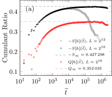
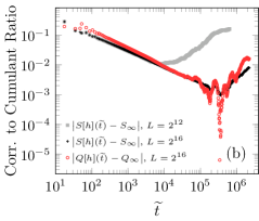
Figure 3: Skewness $S[h]$ and kurtosis $Q[h]$ of the distribution of interface heights in the growth regime. The data belongs to the set of SCA runs with $p=\num{.75}$, $L=2^{16}$ ($n_{\mathrm{\lx@glossaries@gls@link{acronym}{sca}{\leavevmode SCA},p=\num{.75}}}\geq 6430$, compare figure 2). The skewness for a smaller dataset for $L=2^{12}$ ($n_{\mathrm{\lx@glossaries@gls@link{acronym}{sca}{\leavevmode SCA},p=\num{.75},L=2^{12}}}\geq 45$), which reaches the steady state regime at late times in the plot, is included to illustrate finite-size behavior. (a) Cumulant ratios as functions of time. The horizontal lines show the obtained fit parameters for the asymptotic values, to guide the eye. See text for proper values with error estimates. (b) Finite-time and finite-size corrections to the asymptotic values of the cumulant ratios.

In order to get information about the shapes of the distribution of the SCA interface heights we calculated their lowest moments for $L=2^{16}$ and for a smaller $L=2^{12}$, to distinguish finite time from finite size-corrections. Figure 3 shows the evolution of the cumulant ratios $S[h]$ and $Q[h]$, defined by (7) and (8). The curves approach their growth regime asymptotic values, but move away again at late times. These values: $S_{\infty}$ and $Q_{\infty}$ can be determined by performing a fit of the form:

$$R(t)=R_{\infty}+a_{R}/\widetilde{t}^{2\beta}+b_{R}/\widetilde{t}^{4\beta}\quad,$$ (24)

where $\beta$ is the growth exponent, which is motivated by the KPZ ansatz discussed in the next section. We use $\widetilde{t}$, defined in (23), so the timescales match between RS and SCA run across various deposition probabilities. In (34), $R$ is a placeholder for $S[h]$ or $Q[h]$, in the interval: $200\leq\widetilde{t}\leq\SI{200000}{MCS}$, which excludes early time oscillations as well as the cut-off at late times, coming from $\xi\to L$. This yields $S_{\infty}=\num{-0.427}(2)$ and $Q_{\infty}=\num{.352}(3)$ for the growth regime, in agreement with literature values [51, 52, 53, 54] of the KPZ universality class. The sign of $S$ depends on the choice $p\gtrless q$ in the simulations, corresponding to $\operatorname{sign}(\lambda)$ of the KPZ equation (1).

Panel (b) of figure 3 shows the deviations from these asymptotic values. The error estimates given above originate from this representation: The error is assumed to be on the order of the closest approach of the numerical data to the asymptotic value.

After the closest approach to the asymptotic values in the growth regime, $S(\widetilde{t})$ and $Q(\widetilde{t})$, both, move in the direction to their respective values in the steady state: $S_{\infty}\approx\num{.26}$ and $Q_{\infty}\approx\num{.13}$ [42, 55, 56, 57]. The shape of the distribution of surface heights changing in this way is an indication of finite-size effects becoming relevant at $\widetilde{t}_{\mathrm{fs}}\approx\SI{3e5}{MCS}$. This coincides with the time at which the cut-off in $\beta_{\mathrm{eff}}(\widetilde{t})$ was observed in SCA runs for $L=2^{16}$ (see figure 2(b)). Hence it becomes clear, that this change in $\beta_{\mathrm{eff}}$ is caused by finite-size effects. In figure 3(b) we also plotted $S[h](\widetilde{t})$ of a smaller system ($L=2^{12}$), for which the steady state is reached after the relaxation time $\tau=L^{z}\approx\SI{6e5}{MCS}$, but finite-size corrections are evidently relevant long before then.

3.1.2 KPZ ansatz for the growth regime

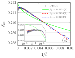
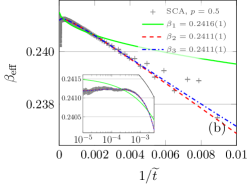
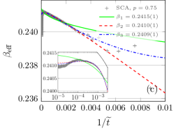
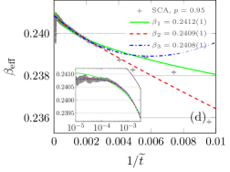
Figure 4: Effective exponents $\beta_{\mathrm{eff}}$ for roughness growth with KPZ ansatz fits using the form (33) to orders one through three. The resulting asymptotic values for $\beta$ are given in the legends accompanied by the uncertainty of the fit parameter. The insets show a zoom to the late-time region $\num{1e-5}\leq 1/\widetilde{t}\leq\num{3e-3}$ (truncated before the finite size break down figure 2(b)). Panel (a) shows the RS dataset using DTrDB. Fits were performed in the interval $\num{1e-5}\leq 1/\widetilde{t}\leq\num{1e-2}$. Panels (b)-(d) show SCA datasets with $p=\num{.5},\num{.75}$ and $\num{.95}$, respectively. The fits were restricted to the interval shown in the inset. The sample size for DTrDB, was $n\geq 1044$. See the captions of figure 2 for other sample sizes.

Analytical and numerical investigations of KPZ models in $1+1$ dimensions found that finite-time corrections to $h(t)$ took the form $\propto t^{-\beta}$ for the interface height [58, 24, 59, 60, 61]:

$$h(t) =\operatorname{sign}(\lambda)\cdot(\Gamma t)^{\beta}\chi+\xi+\zeta t^{-\beta}\quad,$$

where $$\lambda \Gamma \xi \zeta \chi \left\langle h^{n}\right\rangle ~{}\propto t^{-n\beta} ~{}\propto t^{-2\beta}$$, , and are model-dependent parameters and is a universal random variable with Gaussian orthogonal ensemble (GOE) distribution in case of a flat initial condition. The KPZ ansatz hypothesis states, that a generalisation of this form should also hold in higher dimensions [51, 54]. Higher moments of the height show corrections , accordingly, and thus for the roughness, prescribing:

$$\beta_{\mathrm{eff}} =\beta+\sum\limits_{n=1}^{N}c_{n}t^{-2n\beta}\ ,$$ (25)

with non-universal parameters $c_{n}$ and $N$ . Moreover, good agreement between the numerics and experiments has been found  [62, 63, 31]. In the $2+1$ dimensional restricted solid-on-solid model (RSOS) model, the dominant corrections to the roughness growth were found to be of order $~{}\propto t^{-4\beta}$ [54], which motivates the inclusion of higher orders in these forms in higher dimensions [51, 54, 52, 64]. Ideally, such a model would fit the data well as soon as all relevant orders are included. Adding more terms should not improve the fit quality further. However, adding more free parameters in this way can result in overfitting of a noisy data, if not convergence-problems.

Figure 4 shows fitting results using (33) on the previously introduced datasets. It is immediately apparent, that (33) with $N=1$ does not describe the presented data, $n=2$-terms are required, as in case of the RSOS model. In case of RS simulations, the ansatz appears to fit reasonably well early times: $\widetilde{t}\geq 100$ as well. The SCA runs on the other hand show strong oscillations at early times, caused by the synchronous updates, and are not described well by the KPZ ansatz here. Still, late times before the finite size cutoff becomes effective, (in the interval $\num{1e-5}\leq 1/\widetilde{t}\leq\num{3e-3}$) can be fitted well by (33), suggesting universality of the corrections. This becomes true in the $p\to 0$ limit, as in case of figure 2.

The spread of $\beta$ values for larger $N$ provides an estimate for overfitting and may serve as an error estimate for a small confidence interval of $1\sigma$. For simulations with RS dynamics, this yields $\beta=\num{0.2414}(2)$, which, remarkably, is identical to the result based on the average of the late-time plateaus of $\beta_{\mathrm{eff}}$. Fit parameters for $N\leq 6$ can be found in table 3 of the supplemental material.

3.1.3 The KPZ dynamical exponent

The dynamical exponent $z=\alpha/\beta$ of the KPZ class is related to the roughness exponent $\alpha$ by the Galilean symmetry [12]:

$$2=\alpha+z=\alpha\left(1+1/\beta\right)\quad.$$ (26)

Inserting the our estimate $\beta=\num{.2414}(2)$ into this equation yields $\alpha=\num{.3889}(3)$ and $z=\num{1.611}(3)$. The latter is used to calculate autocorrelation exponents in the next section. It should be noted, that the above value for $\alpha$, while in agreement with earlier numerical estimates [42, 50, 65, 64], marginally disagrees with the currently most accepted one $\alpha=\num{.3869}(4)$ [66]. Combining this roughness exponent results with our own estimate for $\beta$ violates equation (26) by about $\num{2.5}\sigma$. A slight violation of the Galilean invariance, which was proposed for discrete systems [67], may explain this disagreement. If this is the case the correct dynamical exponent would be $z=\num{1.603}(3)$. However, the validity of the Galilean invariance is still widely accepted in literature [68, 65, 18], for this reason we use our $\alpha$ and $z$ estimates, obtained using  (26), for consistency.

3.2 Autocorrelation

3.2.1 Autocorrelation of interface heights in the KPZ case

Aging

The autocorrelation results of the interface heights under RS dynamics are summarized in figure 5. A near-perfect collapse of the $C_{h}(t,s)$ functions could be achieved by using $b$ from the relation (14).

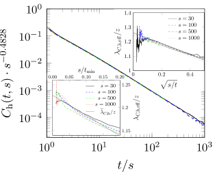
Figure 5: Autocorrelation results from RS calculations using DTrDB. System size $L=2^{16}$, $n\geq 1044$ realizations for $s>30$ and $n\geq 473$ for $s=30$. The main panel shows the collapsed autocorrelation functions for waiting times $s=30,100,500,1000$. Right inset: Corresponding local slope analysis and extrapolations assuming corrections of the form $\sqrt{s/t}$, as drawn. Linear fit was performed for $\sqrt{s/t}\in[\num{.1},\num{.3}]$. Stated errors are pure fit-errors, see text for actual error margins. Left inset: Tail effective exponents obtained from PL fits for intervals $t\geq t_{\mathrm{min}}$ with successively increasing $t_{\mathrm{min}}$. A linear fit to the combination of all curves is displayed as a solid black line, extrapolating to $\widetilde{\lambda}_{C,\mathrm{h}}/z=1.23(3)$.

Autocorrelation exponent obtained by RS dynamics

We calculated effective exponents of $\lambda_{C,h}/z$ and its $t/s\to\infty$ behavior, by an analysis shown in the right inset of figure 5. In order to read-off the appropriate correction to scaling we linearised the left tail of the curves by plotting them on the $\sqrt{s/t}$ scale. This leads to the extrapolations $\lambda_{C,\mathrm{h}}/z=\num{1.254}(9)$ depending on $s$.

To clarify the situation we attempted a different type of local slope analysis presented in the left inset of figure 5, using tail effective exponents, where each $\lambda_{C,\mathrm{h}}/z$ value was determined as the exponent of a PL-fit to $C_{h}(t^{\prime},s)$ for $t^{\prime}\geq t$. These can be expected to converge more monotonically to the asymptotic value as before, because the left tail data of $C_{h}(t,s)$ are included in the procedure for all $t_{\mathrm{min}}$ with an increasing weight as $t_{\mathrm{min}}$ increases. Indeed, the curves of different $s$ values in figure 5(b) behave more linearly with some additional oscillations. However, all curves seem to fluctuate around a common mean, which is not the case for the local slope analysis. A single linear fit for the combination of all curves, yields an averaged extrapolation of $\widetilde{\lambda}_{C,\mathrm{h}}/z=\num{1.23}(3)$ in a marginal agreement with our previous result for this $\lambda_{C,h}/z=1.21(1)$ [30] and with the value obtained in [64, 31] for intermediate times.

The present larger error margin takes the uncertainty due to the actually unknown corrections into account. This problem is illustrated in the comparison between effective exponents and tail effective exponent, where the former show a smaller apparent extrapolation error. In the following we use the simpler extrapolation method based on effective exponents, but estimate the error from their direct fluctuations rather than the uncertainty of the extrapolation fit.

Using our $z$ value the corresponding autocorrelation exponent is $\lambda_{C,\mathrm{heights}}=\num{1.98}(5)$. These results also hold in simulations with more coarse DD, where one would expect an observable difference if any artificial correlations were present.

SCA autocorrelation functions and aging

SCA updates are spatially correlated, therefore they introduce a contribution to the autocorrelation function, which depends on the update probability $p<1$. If we want to model cellular automaton like systems this is not a problem, but for describing the KPZ equation this is artificial. Figure 6 compares the autocorrelation functions of height variables at $p=\num{.95}$ and $p=\num{.5}$. The most apparent property is the finite asymptotic value (figure 6(a)). This is the consequence of frozen regions, arising in ordered domains, which are difficult to randomize by the SCA dynamics. In the dimer model updates can happen at the boundaries only, besides this alternating domains are also stable in case of SCA, they flip-flop at even-odd sublattice steps, when $p\to 1$.

We applied an iterative fitting procedure to determine the functional behavior as follows. As a first approximation the $C_{\mathrm{h}}(t\to\infty,s,p)=o(p)$ limit was determined using a linear extrapolation from the function’s right tail. Subtracting the appropriate value from each curve revealed a PL approach to this constant. To obtain refined $o(p)$ values, the exponent $x$ was read off from the data, allowing a subsequent fit for the tail in the form:

$$f(t)=o+c\cdot t^{-x},$$ (27)

with free parameters $o$ and $c$. The corrected exponents converged as $x^{\prime}\to\lambda_{C}/z$, after subtracting the refined $o(p)$ values. These iterations yielded self-consistent estimates for $o(p)$ and the autocorrelation exponent of the SCA. This procedure is more prone to statistical error for small $t/s$, because $C_{\mathrm{h}}(t,s)$ is farther away from the asymptotic behavior in this case, allowing noise in the tail to influence the extrapolated value more strongly. Table 1 lists the calculated $o(p)$ limits (including those for the lattice-gas variables, see Section 3.2.3).

The limiting value turned out to depend exponentially on $p$. Note, that similar $e^{p}$ dependence has been found in $f_{\mathrm{SCA}}(t,s)$ relating SCA and RS timescales .

Table 1: Autocorrelation limits for KPZ with SCA dynamics for different deposition rates $p$ and $q=0$, as functions of the waiting time $s$. Fit errors are shown, which are below the given number of digits in case of the slopes.

$s/\SI{}{MCS}$	$o_{\mathrm{h}}$		$o_{\mathrm{s}}$
	$p=\num{.5}$	$p=\num{.95}$	$p=\num{.5}$	$p=\num{.95}$
30	0.00320(3)	0.055398(8)	0.012871	0.221623
100	0.00331(5)	0.05520(3)	0.014286	0.219827
500	0.0031(2)	0.05457(8)	0.013944	0.218547
1000	0.0035(3)	0.0548(2)	0.013903	0.218330

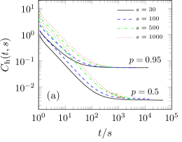
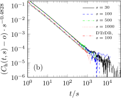
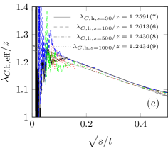
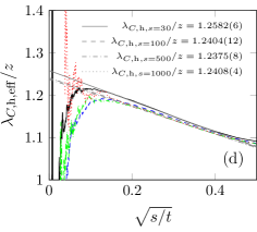
Figure 6: Autocorrelation of KPZ heights from SCA calculations. Error bars have been omitted for clarity. The visible noise is a good indication for $1\sigma$ error. Panels (a) and (b) show data sets with $p=\num{.5}$ (3062 realizations, $t\leq\SI{1.4}{MMCS}$) and $p=\num{.95}$ (3062 realizations, $t\leq\SI{400}{kMCS}$). Lateral system size is $L=2^{16}$. (a): Raw autocorrelation functions showing saturation depending on $p$. (b): Collapsed autocorrelation functions, corrected by the saturation offset $o$ (see text). Plots for $p=\num{.5}$ (lower set of curves) use paler variations of colors than those of $p=\num{.95}$ for the same $s$, to make them distinguishable at late times. The DTrDB autocorrelation function of $s=100$ is also displayed for comparison. The bottom panels (c) and (d), show the local slope analysis corresponding to the $p=\num{.95}$ and $p=\num{.5}$ data sets, respectively. Extrapolations assume corrections of the form $\sqrt{s/t}$, as drawn. Printed error margins are pure fit-errors.

Figure 6(b) shows the corrected $C_{\mathrm{h}}(t,s)$ functions, after subtracting the limiting $o(p)$ values. A nearly perfect data collapse could be achieved using the aging exponent $b_{\mathrm{h}}$, coming from the RS simulations. Even more, the corrected SCA and the displayed RS autocorrelation functions show identical behavior.

Autocorrelation exponent: SCA

Local slope analyses of the corrected autocorrelation functions are displayed in figures 6(c) and 6(d) at $p=\num{.95}$ and $p=\num{.5}$, respectively. Assuming a rescaling of the abscissa: $\sqrt{s/t}$, allows one to observe a linear behavior of the effective exponents for intermediate times. In case of $p=\num{.95}$ the $o$-values could not be determined precisely enough for $s>100$, thus we considered extrapolations at $s=30,100$ only in a weighted average of the results. This yielded: $\lambda_{C,\mathrm{h}}/z=\num{1.26}(1)$ and so $\lambda_{C,\mathrm{h}}=\num{2.01}(2)$. These values are in good agreement with those obtained from a local slope analysis of RS calculations for small $s$.

The effective exponents for $p=\num{.5}$ show a slightly decreasing tendency with $s$ in figure 6(d), moving towards the RS estimate $\widetilde{\lambda}_{C,\mathrm{h}}/z=\num{1.23}(3)$. However, we can’t consider the extrapolated values for $s=500$ and $s=1000$ more precise, than those at $s=30,100$, because the determination of the $o(s)$ constant becomes more uncertain at higher times, increasing the possible error of the exponent estimates.

3.2.2 Autocorrelation of interface heights in the EW case

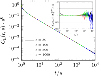
Figure 7: Autocorrelation functions of heights under SCA dynamics with $p=q=\num{.5}$ (EW). Sample size is $n_{\text{\lx@glossaries@gls@link{acronym}{sca}{\leavevmode SCA}}}=5919$. Error bars are omitted for clarity. The magnitude of fluctuations can be seen from the visible fluctuations in the plots. The inset shows the data divided by $C_{\mathrm{h}}^{\mathrm{EW}}$.

Since the autocorrelation function in the EW case is known exactly (22), we can verify our simulations by a comparison with it. Indeed, the expected form could be reproduced by our RS implementation. A more interesting result is, that the SCA simulations also fit it perfectly. The finite saturation value, caused by correlated updates, observed in the KPZ case is not present here.

The agreement with the analytical form is exemplified in the inset of figure 7. A small deviation at very early times can be observed here, as well as in the RS results and should be related to the initial conditions of the simulation with respect to those of the analytical calculations. The application of a fit with  (22) results in $c_{0}\simeq 0.152$ for different waiting times $s$. Using the consistency relation (14) for $s\to t$ we can expect the same value, which was derived for the octahedron model in [38] for the $s\to\infty$ limit.

These numerical results do not only show the correctness of the SCA and RS implementations of the roughening kinetics, but provide an example, where the correlations introduced by SCA do not affect the dynamical behavior.

3.2.3 Autocorrelation of lattice-gas variables in the KPZ case

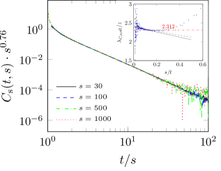
Figure 8: Autocorrelation results from RS calculations using DTrDB (the same runs as those shown figure 5). The main panel shows an aging collapse of the autocorrelation functions for $s=30,100,500,1000$. The inset displays a local slope analysis for $s=30,100$. Linear fitting lines are also shown, assuming corrections of the form ${s/t}$ in the interval $t/s\in[\num{6.25},50]$. The horizontal line ( ) marks the value obtained from direct PL fits.

Next we show results for the lattice-gas variables corresponding to the binary slope values of heights of the KPZ growth presented earlier (see figure 8) using RS dynamics. Here again, the $C_{s}(t,s)$ functions of different waiting times collapse almost perfectly with the value: $b_{\mathrm{s}}=\num{0.76}(2)$. In a previous paper [30] we reported: $b_{\mathrm{s}}=0.70(1)$, which were obtained by a smaller sized analysis.

Autocorrelation exponent: RS

Since the density autocorrelation functions decay much more rapidly than those of the heights, the signal-to-noise ratio in the present sample is insufficient for a reliable extrapolation based on the effective exponents. A weighted average of direct PL fits for $4\leq t/s\leq 90$ yielded $\lambda_{C,\mathrm{s}}/z=\num{2.312}(2)$. However, the effective exponents show curvature as $t/s\to\infty$ and suggest an asymptotic value $\lambda_{C,\mathrm{s,eff}}/z=\num{2.39}(2)$. In [30] we obtained $\lambda_{C,\mathrm{s,eff}}/z=\num{2.35}(2)$, coming from $s=30$, $L=2^{13}$ sized CPU simulations.

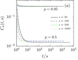
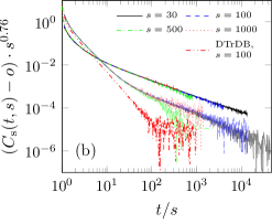
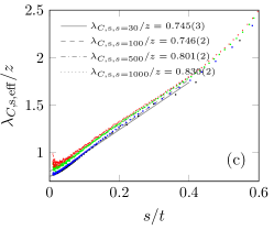
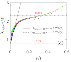
Figure 9: Results from SCA calculations for the autocorrelation of slopes. Error bars have been omitted for clarity. The visible noise is a good indication for $1\sigma$ error. Panels (a) and (b) show data sets with $p=\num{.5}$ and $p=\num{.95}$. Data are taken from the same runs as of figure 6. (a): Raw autocorrelation functions showing saturation depending on $p$. (b): Collapsed autocorrelation functions, corrected by the saturation offset $o$ (see text). The lower set (pale curves) belongs to $p=\num{0.5}$. Data form a DTrDB run for $s=100$ is displayed in red for comparison. The bottom panels (c) and (d), show the local slope analysis corrsponding to the $p=\num{.95}$ and $p=\num{.5}$ data sets, respectively. Extrapolations assume corrections of the form ${s/t}$, as plotted. Printed error margins are pure fit-errors. Horizontal lines ( ) in panel (d) mark the asymptotic esponents for RS updates and SCA at $p=\num{.95}$, from bottom to top.

SCA density autocorrelation functions

Similarly to the case of interface heights the $C_{\mathrm{s}}(t,s)$ functions approach finite values asymptotically, as shown in figure 9(a) as the consequence of the SCA dynamics. The computed values of $o(p,s)$ are listed in table 1.

Figure 9(b) shows the corrected functions $C_{\mathrm{s}}(t,s)-o(p)$ in comparison with our RS result. Data collapse for $p=0.5$ and $p=0.95$ could be achieved using the common aging exponent value $b_{\mathrm{s}}=0.76$, obtained from our previous RS calculations. This indicates, that the density correlation behavior is not changed by the application of SCA updates as in case of the height variables.

SCA density autocorrelation exponent:

In contrast with the interface height results the density correlation exponent of the corrected $C_{\mathrm{s}}(t,s)$ exhibits a more complex behavior. The dataset for $p=\num{.95}$ clearly exhibits a different exponent than what we observed in case of the RS simulations. We show effective exponents fitting for $s=30$ and $100$, where the signal-to-noise ratio is better on figure 9(c). A direct linear fit extrapolating to $s/t\to 0$ yields an estimate of $\lambda_{C,\mathrm{s,\lx@glossaries@gls@link{acronym}{sca}{\leavevmode SCA}}}/z=\num{.75(2)}$.

At $p=\num{.5}$ we can find a crossover form the RS to a different, SCA asymptotic behavior in figure 9(d). A linear extrapolation for the tail of this crossover curve results in $\lambda_{C,\mathrm{s,\lx@glossaries@gls@link{acronym}{sca}{\leavevmode SCA}}}/z$, in good agreement with the $p=\num{.95}$. This leads to the following numerical form for the tail of the autocorrelation function under SCA dynamics:

$$f_{C,\mathrm{\lx@glossaries@gls@link{acronym}{sca}{\leavevmode SCA}}}(t/s,p)\propto c_{1}\cdot(t/s)^{-\lambda_{C,\mathrm{s}}/z}+c_{2}\cdot(t/s)^{-\lambda_{C,\mathrm{s,\lx@glossaries@gls@link{acronym}{sca}{\leavevmode SCA}}}/z}$$ (28)

3.2.4 Autocorrelation of lattice-gas variables in the EW case

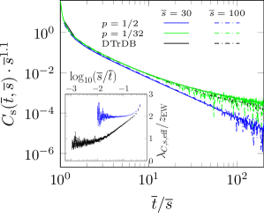
Figure 10: Autocorrelation functions of slopes under SCA (blue and green) and RS (black) dynamics in the linear model. Sample sizes are $n_{\mathrm{\lx@glossaries@gls@link{acronym}{sca}{\leavevmode SCA}},p=\num{.5}}=5919$, $n_{\mathrm{\lx@glossaries@gls@link{acronym}{sca}{\leavevmode SCA}},p=1/32}=147$ and $n_{\mathrm{DTrDB}}=2101$, for both $\overline{s}=30$ and $\overline{s}=100$. For SCA, $p=1/32$, the simulation time is rescaled to collapse the curves, following: $\overline{t}=p\cdot t$, analogously for $s$. No rescaling is applied to the other plots: $\overline{t}=t$. Error bars are omitted for clarity. The magnitude of fluctuations can be seen from the visible fluctuations in the plots. The inset in panel (a) shows the effective autocorrelation exponents $\lambda_{C,\mathrm{s,eff}}/z_{\text{\lx@glossaries@gls@link{acronym}{ew}{\leavevmode EW}}}$ for DTrDB and SCA, $p=1/2$, both for $s=30$ and with $1\sigma$ error bars.

RS autocorrelation functions

In case of RS simulations, the tail of $C_{\mathrm{s}}(t,s)$ does not decay with a simple PL as can be observed in the figure 10. The pronounced curvature in the log-log plot suggests a slower than PL decay at first glance. However, the effective exponents (inset) suggest a PL with an asymptotic exponent $\lambda_{C,\mathrm{s}}^{\text{\lx@glossaries@gls@link{acronym}{ew}{\leavevmode EW}}}/z_{\text{\lx@glossaries@gls@link{acronym}{ew}{\leavevmode EW}}}=\num{0.7}(2)$, following a cross-over from an early-time regime.

SCA autocorrelation functions

While the SCA dynamics seems to reproduce the expected autocorrelation function of the surface heights after the removal of the constant, the evolution of the underlying lattice gas is different. In case of $p=q=\num{.5}$ the density autocorrelation exhibits a PL tail, characterized by $\lambda_{C,\mathrm{s}}^{\text{\lx@glossaries@gls@link{acronym}{sca}{\leavevmode SCA}},\num{.5}}/z_{\text{\lx@glossaries@gls@link{acronym}{ew}{\leavevmode EW}}}\approx 2$ (see inset of figure 10).

In the $p\to 0$ , $q\to 0$ limit the SCA crosses over to an effective RS dynamics, because we avoid the correlated updates of the lattices. This is indeed the case here, evidenced by the $p=q=1/32$ results (see figure 10). Following a rescale of time $t=p\cdot t$ one can find a good collapse with the RS results. Therefore, the update dynamics seems to affect the scaling behavior of the density autocorrelation function.

Aging

The aging exponent obtained from the presented simulations is $b_{\mathrm{s}}^{\text{\lx@glossaries@gls@link{acronym}{ew}{\leavevmode EW}}}=\num{1.1}(2)$. This value holds for both RS and SCA dynamics, but breaks down for very small values of $s$.

4 Discussion and conclusions

We performed extensive simulations of the octahedron model by random-sequential (RS) and stochastic cellular automaton (SCA) dynamics. Precise estimates were obtained for the dynamical behavior: exponents as well as probability distributions of the Kardar–Parisi–Zhang (KPZ) and Edwards–Wilkinson (EW) universality classes. The main advance of this work, in the long story of KPZ research, is the influence of correlated SCA dynamics on the universal properties of these models. Furthermore, we determined the aging properties of the underlying driven lattice gasess (DLGs) of the octahedron model.

By determining moments of the probability distributions we could study finite size effects and arrived at the conclusion that the corrections related to this become relevant much before the occurrence of the steady state. Our surface growth simulations support the validity of the KPZ ansatz hypothesis in $(2+1)D$ and yield a growth exponent $\beta=\num{.2414}(2)$, from which $\alpha=\num{.3889}(3)$ and $z=\num{1.611}(3)$ can be deduced. The growth exponent value lies within the error margins of [57, 52, 50], but not within those of the early landmark result of Forrest and Tang $\beta=\num{.240}(1)$ [69]. However, the small simulation cells used then demanded shorter simulations times, which could have lead to a smaller estimate due finite-time corrections. Under SCA dynamics marginally lower growth exponents were observed for deposition probabilities $p>\num{.5}$ and additional corrections to scaling caused the failure of the KPZ ansatz at early times.

Our estimate of the roughness exponent does not agree with the direct estimate $\alpha=\num{.3869}(4)$, obtained recently through a finite-size scaling analysis of the restricted solid-on-solid model (RSOS) model by Pagnani and Parisi [66], which was based on SCA simulations with $p=\num{0.5}$. Numerical differences between SCA and RS dynamics might be a cause of this. However, since our estimate was derived using (26), a slight violation of the Galilean invariance, which was proposed for discrete systems [67], may also explain this disagreement.

Both our RS and SCA simulations reproduced the expected autocorrelation behavior of interface heights in the EW universality class. In the KPZ case correlated updates resulted in $C_{\mathrm{h}}(t,s)$ to approach a finite value asymptotically. However, after the subtraction of this constant we found the same universal power law (PL) tails for both types of site-selection dynamics.

In case of the underlying lattice-gas variables, we found the relevance of the SCA dynamics for the asymptotic autocorrelation decay exponents, but the aging exponent seems to be insensitive for this. Interestingly, in case of the non-linear (KPZ) model the SCA dynamics slows the decay of the autocorrelations, while in the linear (EW) model this results in a shorter memory of the dimer model. This is the consequence of the effectivity of the ordered SCA updates, which enhances the build up (KPZ) or distortion (EW) of homogeneous areas, correlated for long times.

Our estimates for the autocorrelation exponents of the KPZ class are summarized in table 2. We provided numerical results for $C(t,s)$ in the KPZ case with unprecedented accuracy, drawn from timescales up to $t/s=1000$ due to the high signal-to-noise ratios we could achieve by these parallel algorithms implemented on GPUs. These simulations can be help to test predictions of theories like local scale-invariance with logarithmic corrections [34].

Table 2: Summary of KPZ and EW autocorrelation $\lambda_{C}$ and aging $b$ exponents, assuming $z_{\mathrm{KPZ}}=\num{1.611}(3)$ and $z_{\mathrm{EW}}=2$, respectively. There are no independent estimates for $b$ under SCA dynamics. Values for the EW case provided without error margin correspond to the analytical solution [48, 49].

		$\lambda_{C,\mathrm{h}}$	$\lambda_{C,\mathrm{s}}$	$b_{\mathrm{h}}$	$b_{\mathrm{s}}$
KPZ	RS	1.98(5)	3.8(2)	-.4828(4)	0.76(2)
	SCA	2.01(2)	1.25(2)
EW	RS	2	$\num{1.4}(4)$	0	1.1(2)
	SCA	2	$\approx\num{4}$

The KPZ autocorrelation exponent in $(1+1)$ dimensions was derived analytically $\lambda^{\mathrm{1d}}_{C,\mathrm{h}}=1$ [26, 27]. Later Kallabis and Krug conjectured, that in higher dimensions $\lambda_{C,\mathrm{h}}=D$ [29] applies, but rigourous proof is still missing. Our estimates for $\lambda_{C,\mathrm{h}}$, summarized in table 2, support this hypothesis within error margin both for RS and SCA dynamics.

We have tested the validity of the relation (16) by Krech with our numerical data. The value for the short time dynamical exponent: $\theta=\lambda_{C}/z+2\beta=1.23(2)+0.2414(2)\simeq 1.71(3)$ agrees well with: $(D+4)/z-2=6/1.611(3)-2\simeq 1.72(1)$, therefore we can support the validity of the relation obtained by a perturbative RG analysis [26, 27].

A possible continuation of this work could be the study of the height correlations in the momentum space:

$$C_{q}(t,s)=\left\langle h_{-q}(t)h_{q}(s)\right\rangle\quad.$$

In particular one should be able to test, whether $C_{q}(t,s)$ decays in an exponential or in a stretched exponential way as predicted in references [70, 71, 72, 73]. Note, that we have already succesfully used the extension of the dimer model to determine the power spectrum density: $S(k,t)=\left\langle h_{-q}(t)h_{q}(t)\right\rangle$ in case of Kuramoto-Sivashinsky type of systems [74].

We can also compare the present estimates with our recently published values for the autoresponse $\lambda_{R}=\num{2.00}(6)$ and the corresponding aging exponent $a=0.24(2)$ [33]. $\lambda_{C}\simeq\lambda_{R}$ seems to hold within error margins. In $(1+1)$ dimensions an exceptional fluctuation-dissipation relation (FDR) exists [75, 12]:

$$T\chi(t,s;r)=-\partial^{2}_{r}C(t,s;r)\quad.$$ (29)

This implies the exponent relations $\lambda_{C}=\lambda_{R}$ and

$$1+a=b+2/z$$ (30)

confirmed by simulations [76]. Our $(2+1)D$ results support the first one, but the latter is not satisfied by our numerics:

$$1+a =2\left(\beta+\beta/\alpha\right)$$

$$\num{1.24}(2) \neq\num{1.724}(3)$$

This calls for the existence of a possible FDR in higher dimensions. For example the genaralized form

$$1+a+(D-1)/2=b+2/z$$ (31)

is satisfied by the exponents within error limits in $D=1,2$ both. Confirmation of this assumption should be a target of further research. An intermediate step in this direction could also occur as an inequality, like one found in the KPZ steady state [77, 78].

The autocorrelation and aging exponents which we found for the driven lattice gas of slopes differ from another two dimensional extension of the totally asymmetric exclusion process (TASEP) described in [79], where $\lambda_{C,\mathrm{s}}/z=1$ and $b_{\mathrm{s}}=1$ are reported.

Finally we point out that the SCA simulations are more efficient because they they allow for optimal memory access patters in contrast to the random accesses required for the RS ones. Technical details of our implementations are published elsewhere [43, 44]. The extension of these algorithms for other surface models, like those with conservation laws [74, 80] or in higher dimensions [81] is straightforward. However, the efficiency of RS implementations, using the approach employed here, decreases with the number of dimensions due to the volume of local cells increasing. SCA simulations do not suffer from this problem and are thus more suitable for higher dimensional problems.

The code used in this work can be found at https://github.com/jkelling/CudaKpz.

[Supplemental Information]Supplemental Information:
Dynamical universality classes of simple growth and lattice gas models

Appendix Supplement A Octahedron Model

Figure 11 shows a depiction of the update process in the octahedron model after [38].

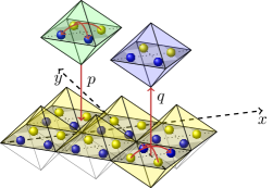
Figure 11: Illustration of the lattice gas (blue and yellow balls) in the $2+1$–dimensional octahedron model. The depiction maps the particles to the up- (blue) and down- (yellow) edges of octahedra. The exchanges of slope-pairs connected to deposition ($p$) and removal ($q$) processes are illustrated. The checkerboard decomposition followed by SCA updates in indicated in the $x$-$y$-plane.

Appendix Supplement B KPZ ansatz for the growth regime

In the main manuscript we test how the KPZ ansatz [58, 24, 60, 59, 51, 52, 64] hypothesis describes the late-time corrections to the growth exponent $\beta$. Its most general form gives

$$\beta_{\mathrm{eff},h} =\beta+\sum\limits_{n=1}^{N}c_{n}t^{-n\beta}\quad,$$ (32)

which for $$N=1 \beta$$ is postulated to describe the corrections to the growth law for the average surface height. Only the special form for the roughness growth, which is reduced to exponents which are even multiples of , was considered in the main text:

$$\beta_{\mathrm{eff}} =\beta+\sum\limits_{n=1}^{N}c_{n}t^{-2n\beta}\quad.$$ (33)

Table 3: Summary of fitting of $\beta_{\mathrm{eff}}$ using the KPZ ansatz in the most general form (32) and using (33) with even powers, more suitable to describe corrections of the roughness-scaling up to maximum orders $N=6$. Error margins given are uncertainties of the fit parameters, not actual error estimates for $\beta$. The reduced sums of residuals $\chi_{\mathrm{red}}$ are given to judge the quality of the fits. For each dataset we underlined the value of $\chi_{\mathrm{red}}$, where the quality does not improve significantly by increasing $N$.

	random-sequential (RS)				stochastic cellular automaton (SCA)
	DTrDB, TC=1,1		DTrDB, TC=2,2		$p=\num{.5}$		$p=\num{.75}$		$p=\num{.95}$
$N$	$\beta$	$\chi_{\mathrm{red}}$	$\beta$	$\chi_{\mathrm{red}}$	$\beta$	$\chi_{\mathrm{red}}$	$\beta$	$\chi_{\mathrm{red}}$	$\beta$	$\chi_{\mathrm{red}}$
equation (32)
$1$	$\num{0.2430}(\num{1})$	10.04	$\num{0.2433}(\num{1})$	9.24	$\num{0.2420}(\num{1})$	7.03	$\num{0.2419}(\num{1})$	8.63	$\num{0.2418}(\num{1})$	3.15
$2$	$\num{0.2396}(\num{1})$	1.82	$\num{0.2396}(\num{1})$	1.29	$\num{0.2403}(\num{1})$	1.62	$\num{0.2400}(\num{1})$	1.31	$\num{0.2403}(\num{1})$	0.51
$3$	$\num{0.2411}(\num{1})$	0.79	$\num{0.2408}(\num{1})$	0.55	$\num{0.2414}(\num{1})$	0.64	$\num{0.2404}(\num{1})$	1.18	$\num{0.2401}(\num{1})$	0.49
$4$	$\num{0.2421}(\num{2})$	0.67	$\num{0.2421}(\num{1})$	0.32	$\num{0.2414}(\num{1})$	0.64	$\num{0.2385}(\num{1})$	0.63	$\num{0.2403}(\num{2})$	0.48
$5$	$\num{0.2386}(\num{3})$	0.47	$\num{0.2409}(\num{2})$	0.28	$\num{0.2388}(\num{3})$	0.51	$\num{0.2394}(\num{3})$	0.61	$\num{0.2399}(\num{5})$	0.48
$6$	$\num{0.2377}(\num{8})$	0.47	$\num{0.2403}(\num{5})$	0.28	$\num{0.2333}(\num{9})$	0.45	$\num{0.2420}(\num{7})$	0.59	$\num{0.2485}(\num{8})$	0.40
equation (33)
$1$	$\num{0.2421}(\num{1})$	7.28	$\num{0.2422}(\num{1})$	6.27	$\num{0.2416}(\num{1})$	5.22	$\num{0.2415}(\num{1})$	6.54	$\num{0.2412}(\num{1})$	1.76
$2$	$\num{0.2414}(\num{1})$	1.16	$\num{0.2414}(\num{1})$	1.10	$\num{0.2411}(\num{1})$	0.65	$\num{0.2410}(\num{1})$	1.72	$\num{0.2409}(\num{1})$	0.81
$3$	$\num{0.2412}(\num{1})$	0.65	$\num{0.2412}(\num{1})$	0.33	$\num{0.2411}(\num{1})$	0.64	$\num{0.2409}(\num{1})$	1.51	$\num{0.2408}(\num{1})$	0.52
$4$	$\num{0.2413}(\num{1})$	0.53	$\num{0.2412}(\num{1})$	0.29	$\num{0.2412}(\num{1})$	0.59	$\num{0.2407}(\num{1})$	0.86	$\num{0.2407}(\num{1})$	0.50
$5$	$\num{0.2412}(\num{1})$	0.51	$\num{0.2412}(\num{1})$	0.28	$\num{0.2412}(\num{1})$	0.59	$\num{0.2406}(\num{1})$	0.68	$\num{0.2405}(\num{1})$	0.41
$6$	$\num{0.2412}(\num{1})$	0.51	$\num{0.2412}(\num{1})$	0.28	$\num{0.2411}(\num{1})$	0.57	$\num{0.2403}(\num{1})$	0.50	$\num{0.2407}(\num{1})$	0.38

A list of best fit parameters for various versions with $N\leq 6$ is provided in table 3, which also lists the reduced sums of residuals $\chi_{\mathrm{red}}$ to quantify agreement between the fitting model and the data.

Where the KPZ ansatz does indeed apply, fits of the more general models (32) should not show increased agreement with the data. The table shows them to be less consistent with respect to the resulting estimates for $\beta$. They provide the best description of the data with only the term $\propto\widetilde{t}^{-2\beta}$, but one or two additional odd terms present ($N=2,3$). The best fits resulting from models (33) are consistently better than those of (32), across all datasets, which justifies discarding the latter class of models and thereby supports the KPZ ansatz hypothesis for the roughness growth.

Appendix Supplement C Distribution of interface heights in the growth regime

In the main manuscript, the finite time corrections to the cumulant ratio of the distribution of surface heights are shown to be described by the KPZ ansatz, yielding the form:

$$R_{\mathrm{KPZ}}(t) =R_{\infty}+a_{R}\cdot\widetilde{t}^{\beta}+b_{R}\cdot\widetilde{t}^{2\beta}\quad.$$ (34)

Assuming a single PL in the form:

$$R(t) =R_{\infty}+a_{R}\cdot\widetilde{t}^{c_{R}}\quad,$$ (35)

a fit can also be made, resulting in the exponents $c_{S}\approx\num{-.54}$ and $c_{Q}\approx\num{-.60}$ for $S[h](t)$ and $Q[h](t)$, respectively. The value $c_{R}\approx\num{-.6}$ also holds for a number of other dimensionless cumulant rations, not displayed here. The values for $S_{\infty}$ and $Q_{\infty}$ resulting from this extrapolation stay well within the margins of error given in the main manuscript.

References

- [1] Marro J and Dickman R 2005 Nonequilibrium Phase Transitions in Lattice Models Collection Alea-Saclay: Monographs and Texts in Statistical Physics (Cambridge University Press) ISBN 9780521019460
- [2] Krug J 1997 Adv. Phys. 46 139–282
- [3] Halpin-Healy T and Zhang Y C 1995 Physics Reports 254 215–414 ISSN 0370-1573
- [4] Täuber U C 2014 Critical Dynamics (Cambridge University Press) ISBN 9781139046213 cambridge Books Online
- [5] Ódor G 2008 Universality in Nonequilibrium Lattice Systems (World Scientific)
- [6] Spitzer F 1970 Advances in Mathematics 5 246–290 ISSN 0001-8708
- [7] Meakin P, Ramanlal P, Sander L M and Ball R C 1986 Phys. Rev. A 34(6) 5091–5103
- [8] Plischke M, Rácz Z and Liu D 1987 Phys. Rev. B 35(7) 3485–3495
- [9] Kardar M, Parisi G and Zhang Y C 1986 Phys. Rev. Lett. 56(9) 889–892
- [10] Burgers J M 1974 The nonlinear diffusion equation : asymptotic solutions and statistical problems (Dordrecht-Holland ; Boston : D. Reidel Pub. Co) ISBN 9027704945 first published in 1973 under title: Statistical problems connected with asymptotic solutions of the one-dimensional nonlinear diffusion equation
- [11] Halpin-Healy T 1990 Phys. Rev. A 42(2) 711–722
- [12] Forster D, Nelson D R and Stephen M J 1977 Phys. Rev. A 16(2) 732–749
- [13] Kardar M 1985 Phys. Rev. Lett. 55(26) 2923–2923
- [14] van Beijeren H, Kutner R and Spohn H 1985 Phys. Rev. Lett. 54(18) 2026–2029
- [15] Janssen H and Schmittmann B 1986 Zeitschrift für Physik B Condensed Matter 63 517–520 ISSN 0722-3277
- [16] Hwa T 1992 Phys. Rev. Lett. 69(10) 1552–1555
- [17] Edwards S F and Wilkinson D R 1982 Proc. R. Soc. London, Ser. A 381 17–31 ISSN 0080-4630
- [18] Barabási A and Stanley H 1995 Fractal Concepts in Surface Growth (Cambridge University Press) ISBN 9780521483186
- [19] Family F and Vicsek T 1985 J. Phys. A 18 L75
- [20] Marinari E, Pagnani A, Parisi G and Rácz Z 2002 Phys. Rev. E 65(2) 026136
- [21] Foltin G, Oerding K, Rácz Z, Workman R L and Zia R K P 1994 Phys. Rev. E 50(2) R639–R642
- [22] Calabrese P and Le Doussal P 2011 Phys. Rev. Lett. 106(25) 250603
- [23] Prähofer M and Spohn H 2000 Phys. Rev. Lett. 84(21) 4882–4885
- [24] Sasamoto T and Spohn H 2010 Phys. Rev. Lett. 104(23) 230602
- [25] Barrat J L, Feigelman M, Kurchan J and Dalibard J 2003 Slow Relaxations and Nonequilibrium Dynamics in Condensed Matter (Les Houches - Ecole d’Ete de Physique Theorique vol 77) (Springer) ISBN 978-3-540-40141-4
- [26] Krech M 1997 Phys. Rev. E 55(1) 668–679
- [27] Krech M 1997 Phys. Rev. E 56(1) 1285–1285
- [28] Kloss T, Canet L and Wschebor N 2012 Phys. Rev. E 86(5) 051124
- [29] Kallabis H and Krug J 1999 EPL 45 20
- [30] Ódor G, Kelling J and Gemming S 2014 Phys. Rev. E 89(3) 032146
- [31] Carrasco I S S, Takeuchi K A, Ferreira S C and Oliveira T J 2014 New J. Phys. 16 123057
- [32] Henkel M and Pleimling M 2010 Non-Equilibrium Phase Transitions: Volume 2: Ageing and Dynamical Scaling Far from Equilibrium Theoretical and Mathematical Physics (Springer Netherlands) ISBN 9789048128686
- [33] Kelling J, Odor G and Gemming S 2017 Journal of Physics A: Mathematical and Theoretical
- [34] Henkel M 2013 Nucl. Phys. B 869 282–302 ISSN 0550-3213
- [35] Henkel M 2017 Symmetry 9 2 ISSN 2073-8994 URL http://www.mdpi.com/2073-8994/9/1/2
- [36] Durang X and Henkel M 2017 ArXiv e-prints (Preprint 1708.08237)
- [37] Krug J and Spohn H 1991 Kinetic roughening of growing surfaces Solids Far From Equilibrium: Growth, Morphology and Defects ed Godreche C (Cambridge University Press) pp 479–582
- [38] Ódor G, Liedke B and Heinig K H 2009 Phys. Rev. E 79 021125
- [39] Rajewsky N, Santen L, Schadschneider A and Schreckenberg M 1998 J. Stat. Phys. 92 151–194 ISSN 0022-4715
- [40] Schulz H, Ódor G, Ódor G and Nagy M F 2011 Comp. Phys. Comm. 182 1467–1476
- [41] Juhász R and Ódor G 2012 Journal of Statistical Mechanics: Theory and Experiment 2012 P08004
- [42] Marinari E, Pagnani A and Parisi G 2000 J. Phys. A 33 8181
- [43] Kelling J, Ódor G and Gemming S 2016 Bit-Vectorized GPU Implementation of a Stochastic Cellular Automaton Model for Surface Growth 2016 IEEE International Conference on Intelligent Engineering Systems, 2016. INES ’16 (IEEE)
- [44] Kelling J, Ódor G and Gemming S 2017 Computer Physics Communications 220 205–211 ISSN 0010-4655 URL http://www.sciencedirect.com/science/article/pii/S0010465517302175
- [45] Levenberg K 1944 Q. J. Appl. Math. II 164–168
- [46] Marquardt D W 1963 Journal of the Society for Industrial and Applied Mathematics 11 431–441 (Preprint http://dx.doi.org/10.1137/0111030)
- [47] Williams T, Kelley C, Bersch C, Bröker H B, Campbell J, Cunningham R, Denholm D, Elber G, Fearick R, Grammes C, Hart L, Hecking L, Juhász P, Koenig T, Kotz D, Kubaitis E, Lang R, Lecomte T, Lehmann A, Lodewyck J, Mai A, Märkisch B, Merritt E A, Mikulı´k P, Steger C, Takeno S, Tkacik T, der Woude J V, Zandt J R V, Woo A and Zellner J 2015 Gnuplot: an interactive plotting program http://www.gnuplot.info
- [48] Röthlein A, Baumann F and Pleimling M 2006 Phys. Rev. E 74(6) 061604
- [49] Röthlein A, Baumann F and Pleimling M 2007 Phys. Rev. E 76(1) 019901(E)
- [50] Kelling J and Ódor G 2011 Phys. Rev. E 84(6) 061150
- [51] Halpin-Healy T 2012 Phys. Rev. Lett. 109(17) 170602
- [52] Halpin-Healy T 2013 Phys. Rev. E 88(4) 042118
- [53] Alves S G and Ferreira S C 2012 Journal of Statistical Mechanics: Theory and Experiment 2012 P10011
- [54] Oliveira T J, Alves S G and Ferreira S C 2013 Phys. Rev. E 87(4) 040102
- [55] Paiva T and Aarão Reis F 2007 Surf. Sci. 601 419–424 ISSN 0039-6028
- [56] Aarão Reis F D A 2004 Phys. Rev. E 69(2) 021610
- [57] Kelling J, Ódor G and Gemming S 2016 Phys. Rev. E 94(2) 022107
- [58] Ferrari P L and Frings R 2011 J. Stat. Phys. 144 1123 ISSN 1572-9613
- [59] Alves S G, Oliveira T J and Ferreira S C 2014 Phys. Rev. E 90(2) 020103
- [60] Alves S G, Oliveira T J and Ferreira S C 2013 Journal of Statistical Mechanics: Theory and Experiment 2013 P05007
- [61] Halpin-Healy T and Lin Y 2014 Phys. Rev. E 89(1) 010103
- [62] Takeuchi K A and Sano M 2010 Phys. Rev. Lett. 104(23) 230601
- [63] Takeuchi K A and Sano M 2012 Journal of Statistical Physics 147 853–890 ISSN 1572-9613
- [64] Halpin-Healy T and Palasantzas G 2014 EPL 105 50001
- [65] Rodrigues E A, Mello B A and Oliveira F A 2015 J. Phys. A 48 035001
- [66] Pagnani A and Parisi G 2015 Phys. Rev. E 92(1) 010101
- [67] Wio H S, Revelli J A, Deza R R, Escudero C and de la Lama M S 2010 EPL 89 40008
- [68] Kloss T, Canet L and Wschebor N 2012 Phys. Rev. E 86(5) 051124
- [69] Forrest B M and Tang L H 1990 Phys. Rev. Lett. 64(12) 1405–1408
- [70] Schwartz M and Edwards S 2002 Physica A: Statistical Mechanics and its Applications 312 363–368 ISSN 0378-4371
- [71] Edwards S F and Schwartz M 2002 Physica A: Statistical Mechanics and its Applications 303 357–386 ISSN 0378-4371 URL http://www.sciencedirect.com/science/article/pii/S0378437101004794
- [72] Colaiori F and Moore M A 2001 Phys. Rev. E 63(5) 057103 URL https://link.aps.org/doi/10.1103/PhysRevE.63.057103
- [73] Katzav E and Schwartz M 2004 Phys. Rev. E 69(5) 052603
- [74] Ódor G, Liedke B and Heinig K H 2010 Phys. Rev. E 81(5) 051114
- [75] Deker U and Haake F 1975 Phys. Rev. A 11(6) 2043–2056
- [76] Henkel M, Noh J D and Pleimling M 2012 Phys. Rev. E 85(3) 030102
- [77] Katzav E and Schwartz M 2011 EPL (Europhysics Letters) 95 66003 URL http://stacks.iop.org/0295-5075/95/i=6/a=66003
- [78] Katzav E and Schwartz M 2011 Phys. Rev. Lett. 107(12) 125701 URL https://link.aps.org/doi/10.1103/PhysRevLett.107.125701
- [79] Daquila G L and Täuber U C 2011 Phys. Rev. E 83(5) 051107
- [80] Ódor G, Liedke B, Karl-Heinz H and Kelling J 2012 Applied Surface Science 258
- [81] Ódor G, Liedke B and Heinig K H 2010 Phys. Rev. E 81(3) 031112