Diffusion dominated evaporation in multicomponent lattice Boltzmann simulations

Abstract

We present a diffusion dominated evaporation model using the popular pseudopotential multicomponent lattice Boltzmann method introduced by Shan and Chen. With an analytical computation of the diffusion coefficients, we demonstrate that Fick’s law is obeyed. We then validate the applicability of our model by demonstrating the agreement of the time evolution of the interface position of an evaporating planar film to the analytical prediction. Furthermore, we study the evaporation of a freely floating droplet and confirm that the effect of Laplace pressure is significant for predicting the time evolution of small droplet radii.

I Introduction

Evaporating fluids are ubiquitous in our daily life and in industrial processes, such as ink jet printing Lei2015 , coating Nadir2015 and particle deposition Wei2012 . In particular for suspensions or polymer solutions, as well as fluids in confined geometries, the evaporation of individual components can induce fluid flows or a change of relative concentrations leading to changing rheological and transport properties of the constituents. For example, the evaporation of a sessile colloidal droplet on a substrate leads to a capillary flow transporting the colloidal particles to the edge of a droplet, which finally results in a ring-like deposit Deegan1997 . The ring-like stains can be a useful tool to deposit particles and can also be disadvantageous when a uniform pattern is desirable. Another example is the evaporation of droplets on rough or chemically patterned substrates. Surrounding geometries and the wettability of a substrate have a large influence on the lifetime of evaporating droplets GelMarNai11 . A thorough understanding of this impact of evaporation on the fluid behavior is mandatory to consequently optimize industrial applications and to improve our fundamental understanding of effects like film formation, droplet drying, or droplet spreading.

There are numerous theoretical EpsPle50 ; Popov2005 ; Stephen2015 and experimental Deegan1997 ; Marin2011 studies of fluid evaporation. While most theoretical studies are limited to the macroscopic scale, experiments suffer from difficulties that arise by tuning the individual microscale properties of fluids. The thorough understanding of fluid evaporation calls for mesoscopic or microscopic details and the flexibility to tune the properties of individual fluid constituents independently. This is possible by means of computer simulations. Computer simulations allow access to parameters which are not easily controllable in experiments and to tune the properties of individual fluid constituents independently. They can thus help to improve our understanding of evaporation driven fluid transport. Simulations of evaporating fluids often utilize molecular dynamics (MD) Long1996 ; WangMD2013 ; Chen2013 ; Detlef2015 . While MD offers a very high flexibility in the microscopic details, its computational cost is very high. Therefore, MD simulations are limited to very small length and time scales on the nanometre or nanosecond scale Detlef2015 . In order to reach experimentally relevant scales, a continuum approach is more productive and our method of choice is the lattice Boltzmann method (LBM) Succi2001 ; BenSucSau92 ; Raa04 . The LBM has gained popularity for the simulation of fluid flows due to its straightforward implementation and parallelization. Soon after its invention, the LBM was extended to simulate multiple interacting fluid phases and components and today a plethora of multiphase and multicomponent methods exists Liu2016 ; Shan1993 ; Gunstensen1991 ; Swift1995 ; He1999 ; Falcucci2011 .

The mesoscale nature of the method combined with the possibility to add additional fields, external forces, suspended objects, thermal noise, or complex boundary conditions in a very straightforward manner has made the LBM particularly popular for applications in microfluidics and soft matter physics. Many of the physical systems studied in these fields include volatile liquids, where the effect of evaporation plays a dominant role. Therefore, it is not surprising that a number of groups has simulated evaporating fluids using the LBM recently. Ledesma-Aguilar et al. LedVelYeo14 ; AguVelYeo16 present a diffusion based evaporation method based on the free energy multiphase lattice Boltzmann method and demonstrate quantitative agreement with several benchmark cases as well as qualitative agreement with the experimental data of evaporating droplet arrays. Jansen et al. Jansen2013 study the evaporation of droplets on a chemically patterned substrate and qualitatively compare the simulation results with experimental data. Their method is based on a continuous removal of mass from the droplet and thus does not allow studying transport processes in the vapor phase. Yan et al. Qing2016 present a thermal model to study the contact line dynamics during droplet evaporation where the liquid-vapor phase change is driven by a temperature field and a well defined equation of state. Joshi and Sun Joshi2010 present simulations of drying colloidal suspensions by means of a modified pseudopotential multiphase model following Shan and Chen. They assign a fixed mass flux to the system boundary which causes a reduction in vapor concentration and thus triggers a liquid-vapor phase change at the interface. However, their results are purely qualitative and a thorough analytical understanding of the diffusion in the system is missing.

In this paper we overcome this limitation and introduce an alternative evaporation model for the pseudopotential method of Shan and Chen. We focus on the two-component version of the method Shan1993 , but the application to an arbitrary number of components and the multiphase pseudopotential method is straightforward. Generally, the pseudopotential LBM is very popular due to its ease of implementation and flexibility when combined for example with complex geometries Martys1996a ; Liu2016 , locally varying contact angles HarKunHer06 , or suspended particles JanHar11 . To trigger evaporation, we do not impose a mass flux, but instead fix the density of one component at selected boundary sites which induces a density gradient. The evaporation process is diffusion dominated and can be well described using Fick’s law with well defined diffusivities. We validate the applicability of our model by comparing the time dependent simulation results of an evaporating planar film and a freely floating evaporating droplet with their respective analytical predictions.

This remainder of this paper is organised as follows. Sec. II introduces the lattice Boltzmann method and our extension for evaporating fluids. Our results are shown in Sec. III and Sec. IV concludes the article.

II Simulation method

II.1 The lattice Boltzmann method

The lattice Boltzmann equation can be obtained from spatially and temporally discretizing the Boltzmann equation. Multiple fluid components $c$ are modeled by following the evolution of the single particle distribution function

$$f_{i}^{c}(\mathbf{x}+\mathbf{e}_{i}\Delta t,t+\Delta t)-f_{i}^{c}(\mathbf{x},t)= -\frac{\Delta t}{\tau^{c}}[f_{i}^{c}(\mathbf{x},t)$$

$$-f_{i}^{\mathrm{eq}}(\rho^{c}(\mathbf{x},t),\mathbf{u}^{c}_{eq}(\mathbf{x},t))]\mbox{.}$$ (1)

The single particle distribution functions $f_{i}^{c}(\mathbf{x},t)$ at positions $\mathbf{x}$ alternatively stream, as described by the LHS of (1), along the $i=1,\ldots,19$ discretized directions $\mathbf{e}_{i}$ and collide, as described by the RHS of (1) at every timestep $t$. Throughout this work we utilize $2$ components $c$ and $\overline{c}$. The collision is achieved by relaxing the probability distribution functions towards a discretized second-order equilibrium distribution function

$$f_{i}^{\mathrm{eq}}(\rho^{c},\mathbf{u}^{c}_{eq})=\omega_{i}\rho^{c}\bigg{[}1+\frac{\mathbf{c}_{i}\cdot\mathbf{u}^{c}_{eq}}{c_{s}^{2}}-\frac{\left(\mathbf{u}^{c}_{eq}\cdot\mathbf{u}^{c}_{eq}\right)}{2c_{s}^{2}}$$

$$+\frac{\left(\mathbf{c}_{i}\cdot\mathbf{u}^{c}_{eq}\right)^{2}}{2c_{s}^{4}}\bigg{]}\mbox{,}$$ (2)

where $c_{s}=\frac{1}{\sqrt{3}}\frac{\Delta x}{\Delta t}$ is the speed of sound and $\omega_{i}$ is a weight factor defined as $\omega_{0}=\frac{1}{3}$, $\omega_{1,\ldots,6}=\frac{1}{18}$ and $\omega_{7,\ldots,18}=\frac{1}{36}$. The densities are defined as $\rho^{c}(\mathbf{x},t)=\rho_{0}\sum_{i}f^{c}_{i}(\mathbf{x},t)$, where $\rho_{0}$ is a reference density, and the velocities are defined as $\mathbf{u}^{c}(\mathbf{x},t)=\sum_{i}f^{c}_{i}(\mathbf{x},t)\mathbf{c}_{i}/\rho^{c}(\mathbf{x},t)$, while the velocity in the equilibrium distribution function is $\mathbf{u}^{c}_{eq}=\sum_{c}\rho^{c}u^{c}/\sum_{c}\rho^{c}$.

For brevity and numerical efficiency we choose the lattice constant $\Delta x$, the timestep $\Delta t$, the unit mass $\rho_{0}$ and the relaxation time $\tau^{c}$ to be unity, which leads to a kinematic viscosity $\nu^{c}$ $=\frac{2\tau-1}{6}=\frac{1}{6}$ in lattice units.

The system boundaries are treated as periodic boundaries by default. To do so, fluid leaving one system boundary reenters the opposite side and forces are computed across these periodic boundaries. To inhibit flow walls can be constructed by inverting velocities at selected boundary sites Succi2001 .

II.2 The pseudopotential multicomponent lattice Boltzmann method

For the fluid components introduced above to become immiscible, Shan and Chen introduced a pseudopotential interaction force

$$\mathbf{F}^{c}(\mathbf{x},t)=-\Psi^{c}(\mathbf{x},t)\sum_{\bar{c}}\sum_{i}\omega_{i}g^{c\bar{c}}\Psi^{\bar{c}}(\mathbf{x}+\mathbf{e}_{i},t)\mathbf{e}_{i}\,\,\,$$ (3)

to achieve separation of the components Shan1993 . This force is defined as a nearest neighbor interaction between fluid components $c$ and $\bar{c}$ Shan1993 and scaled through the choice of the parameter $g^{c\bar{c}}$. Here $\Psi^{c}(\mathbf{x},t)$ is an effective mass, defined as

$$\Psi^{c}(\mathbf{x},t)\equiv\Psi(\rho^{c}(\mathbf{x},t))=1-e^{-\rho^{c}(\mathbf{x},t)/\rho_{0}}\mbox{.}$$ (4)

The force is applied to the fluid by adding a shift of $\Delta\mathbf{u}^{c}(\mathbf{x},t)=\frac{\tau^{c}\mathbf{F}^{c}(\mathbf{x},t)}{\rho^{c}(\mathbf{x},t)}$ to $\mathbf{u}^{c}_{eq}(\mathbf{x},t)$ during collision. This causes the separation of fluids and the formation of a diffuse interface between them. The width of the interface separating the regions is typically about $5\Delta x$ Frijters2012 , with a small dependence on the interaction strength.

II.3 The evaporation model

When the interaction parameter $g^{c\bar{c}}$ in the pseudopotential model is properly chosen Martys1996a , a separation of components takes place. Each component will separate into a denser majority phase of density $\rho_{ma}$ and a lighter minority phase of density $\rho_{mi}$, respectively.

In order to drive the system out of equilibrium, we impose the density of component $c$ at the boundary sites $\mathbf{x}_{H}$ to be of constant value $\rho^{c}(\mathbf{x}_{H},t)=\rho^{c}_{H}$ by setting the distribution function of component $c$ to

$$f_{i}^{c}(\mathbf{x}_{H},t)=f_{i}^{\mathrm{eq}}\left(\rho_{H}^{c},\mathbf{u}^{c}_{H}(\mathbf{x}_{H},t)\right),$$ (5)

in which $\mathbf{u}^{c}_{H}(\mathbf{x}_{H},t)=0$. Setting the velocity to zero at the system boundary is in agreement with the idea of an undisturbed large volume outside the system, which does not cause perturbations in the system. Depending on the ratio of the minority density $\rho^{c}_{mi}$ and $\rho_{H}^{c}$ this induces evaporation or condensation. Furthermore, for simplicity, we ensure total mass conservation within the system by setting the density of component $\bar{c}$ as

$$\rho^{\bar{c}}(\mathbf{x}_{H},t)=\rho^{c}(\mathbf{x}_{H},t-1)+\rho^{\bar{c}}(\mathbf{x}_{H},t-1)-\rho^{c}_{H}$$ (6)

and again ensure an undisturbed flow field by setting $\mathbf{u}^{\bar{c}}_{H}(\mathbf{x}_{H},t)=0$, so that the distribution functions of component $\bar{c}$ at the evaporation boundary sites $\mathbf{x}_{H}$ become

$$f_{i}^{\bar{c}}(\mathbf{x}_{H},t)=f_{i}^{\mathrm{eq}}\left(\rho_{H}^{\bar{c}},\mathbf{u}^{\bar{c}}_{H}(\mathbf{x}_{H},t)\right).$$ (7)

We note that our model can be easily extended to situations where mass is not conserved. We ensure the equivalence to the open system by mimicking a zero density gradient within the infinite volume outside the system. This way forces from the pseudopotential interactions only have an impact in the bulk of the simulation volume and not at the boundary. This can be achieved either by using evaporation boundaries on periodic sites as well or by using a second layer of evaporation boundary sites. Thereby we enforce the same density and a zero gradient at the system boundary.

In the case where the set density $\rho_{H}^{c}$ is not equal to the equilibrium minority density $\rho_{mi}^{c}$, a density gradient in the vapor phase of component $c$ is formed. This gradient causes component $c$ to diffuse towards the minimum.

III Results and Discussions

III.1 Diffusion

In binary fluid mixtures, following Fick’s first law, we can write the mass flux of component $c$ as

$$\mathbf{j}^{c}=-D^{cc}\nabla\rho^{c}-D^{c{\bar{c}}}\nabla\rho^{\bar{c}},$$ (8)

where $D^{cc}$, $D^{c{\bar{c}}}$ are the diffusion coefficients. In the Shan-Chen multicomponent method, the mass flux of component $c$ can be written as Shan1996

$$\mathbf{j}^{c}=\rho^{c}(\mathbf{U}^{c}-\mathbf{U}),$$ (9)

where $\mathbf{U}^{c}$ and $\mathbf{U}$ are macroscopic velocities of component $c$ and the binary mixture, respectively. The macroscopic velocities are defined as an average of the total momentum before and after each collision Shan1995a as

$$\mathbf{U} = \frac{\rho^{c}\mathbf{u}^{c}+\rho^{\bar{c}}\mathbf{u}^{\bar{c}}+\frac{1}{2}(\mathbf{F}^{c}+\mathbf{F}^{\bar{c}})}{\rho^{c}+\rho^{\bar{c}}}\mbox{,}$$ (10)

$$\mathbf{U^{c}} = \frac{1}{2\rho^{c}}\left[\rho^{c}\mathbf{u}^{c}+\mathbf{F}^{c}+\frac{\rho^{c}(\rho^{c}\mathbf{u}^{c}+\rho^{\bar{c}}\mathbf{u}^{\bar{c}})}{\rho^{c}+\rho^{\bar{c}}}\right]\mbox{.}$$ (11)

By performing a Chapman-Enskog expansion Shan1995a , Eq. (9) can be rewritten to be identical to Eq. (8), with the diffusion coefficients given as Shan1996

$$\!\!\!D^{cc} = c_{s}^{2}\left(\tau-\frac{1}{2}\right)\frac{\rho^{\bar{c}}}{\rho^{c}+\rho^{\bar{c}}}-\frac{c_{s}^{2}\rho^{c}\Psi^{\bar{c}}g^{\bar{c}c}\Psi^{{}^{\prime}c}}{\rho^{c}+\rho^{\bar{c}}},$$

$$\!\!\!D^{c{\bar{c}}} = -c_{s}^{2}\left(\tau-\frac{1}{2}\right)\frac{\rho^{c}}{\rho^{c}+\rho^{\bar{c}}}+\frac{c_{s}^{2}\rho^{\bar{c}}\Psi^{c}g^{c\bar{c}}\Psi^{{}^{\prime}\bar{c}}}{\rho^{c}+\rho^{\bar{c}}},$$ (12)

with $\Psi^{{}^{\prime}c}$ being the spatial derivative of $\Psi^{c}$. We note that the diffusion is dependent on the symmetric interaction strengths $g^{c\bar{c}}$ and $g^{\bar{c}c}$, as well as the densities of the two components $\rho^{c}$ and $\rho^{\bar{c}}$.

In the limit of small gradients, we can assume that $\nabla\rho^{\bar{c}}(\mathbf{x},t)=-\nabla\rho^{c}(\mathbf{x},t)$, with which Eq. (8) becomes

$$\mathbf{j}^{c}=-D^{c}\nabla\rho^{c},$$ (13)

where

$$\!\!\!\!\!\!\!\!\!\!\!\!\!\!\!\!D^{c}=\biggl{[}c_{s}^{2}(\tau-\frac{1}{2})-\frac{c_{s}^{2}}{\rho^{c}+\rho^{\bar{c}}}(\rho^{\bar{c}}\Psi^{c}g^{c\bar{c}}\Psi^{{}^{\prime}\bar{c}}+\rho^{c}\Psi^{\bar{c}}g^{\bar{c}c}\Psi^{{}^{\prime}c})\biggr{]}.$$ (14)

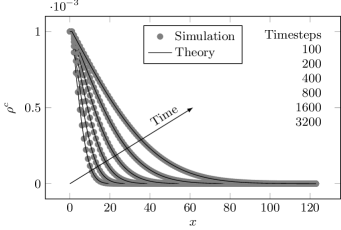
Figure 1: Time evolution of density profiles of component $c$. The system is initially empty of $c$. Diffusion allows fluid from an infinite reservoir at $x=0$ to build up gradually changing density profiles in agreement with the analytical solution.

To validate the theoretical analysis above, we investigate the diffusion of a component $c$ into a system filled with another component $\bar{c}$. We perform a simulation with a system size of $125\times 4\times 4$ and fill the system with fluid $\bar{c}$ of density $\rho^{\bar{c}}=0.7$. A wall of thickness $h=2$ is placed at $x=125$ and the fluid interaction parameter is set to $g^{c\bar{c}}=g^{\bar{c}c}=3.6$. We utilize an evaporation boundary at $x=0$ and set the density $\rho^{c}_{H}=0.001$ to ensure a diffusive flow that is undisturbed by convection. Then component $c$ diffuses into the system. Meanwhile, we numerically solve Fick’s second law

$$\frac{\partial\rho^{c}}{\partial t}=-D^{cc}\Delta\rho^{c}-D^{c{\bar{c}}}\Delta\rho^{\bar{c}}$$

$$\frac{\partial\rho^{\bar{c}}}{\partial t}=-D^{\bar{c}\bar{c}}\Delta\rho^{\bar{c}}-D^{{\bar{c}}c}\Delta\rho^{c}$$ (15)

to describe the space and time dependent density profile of component $c$. In Fig. 1 we compare the lattice Boltzmann simulation results (symbols) with the numerical solution of Eq. (15) (solid lines). From the evaporation boundary with density $\rho_{H}^{c}$ fluid diffuses into the system. Being a diffusion process, the rate at which the fluid invades the system is dependent on the density gradient. The gradient subsequently decreases and fluid distributes itself further into the system, aiming to remove the gradient. There is a good agreement between simulation results and the numerical solution, as shown in Fig. 1.

We note that the diffusion equation does not hold at fluid-fluid interfaces Shan1996 . However, the movement of the interface during evaporation is governed by diffusion of the fluids surrounding it, which we demonstrate as follows.

III.2 Evaporation of a planar film

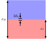
Figure 2: (Color online) Schematic representation of the planar film (front view). We fill the lower half of the system with fluid $c$ and the upper half with fluid $\overline{c}$ such that a fluid-fluid interface forms at $x_{I}$. The interface thickness is $2d_{0}$. To drive the evaporation we impose the boundary condition $\rho^{c}(x=x_{H})=\rho^{c}_{H}$ at the top of the system. A solid surface with thickness $h=2$ is located at the bottom.

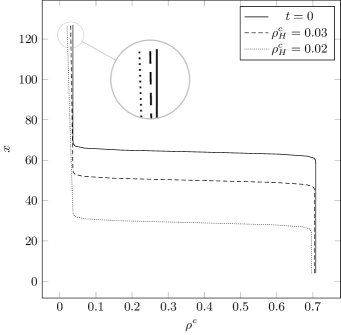
Figure 3: Density profile of fluid $c$ along the $x$ direction after equilibration (defined as $t=0$, solid line) and density profiles at $t=10^{6}$ timesteps later with boundary densities $\rho^{c}_{H}=0.03$ (dashed line) and $\rho^{c}_{H}=0.02$ (dotted line). The magnification depicts of the subtle difference of $\rho^{c}_{H}$ causing a different density gradient and a different time behavior of the moving interface.

We investigate the evaporation of a planar film sitting on a solid substrate, as illustrated in  Fig. 2. To do so we perform simulations with a system size of $128\times 4\times 4$. We fill one half of the system with fluid $c$ and the other half with fluid $\bar{c}$ of equal density ($\rho^{c}_{ma}=\rho^{\bar{c}}_{ma}=0.70$, $\rho^{c}_{mi}=\rho^{\bar{c}}_{mi}=0.04$) such that a fluid-fluid interface forms at $x_{0}=64$. We define the position of the interface $x_{I}$ as the position of $\rho^{c}-\rho^{\bar{c}}=0$. The interaction strength in Eq. (3) is chosen to be $g^{c\bar{c}}=g^{\bar{c}c}=3.6$. We place a wall of thickness $2$ with simple bounce back boundary conditions at the bottom, parallel to the interface, while the boundaries normal to the substrate are periodic.

After equilibration the density of fluid $c$ is constant in both the denser phase ($\rho^{c}_{ma}\approx 0.704$) and the lighter phase ($\rho^{c}_{mi}\approx 0.036$), whereas between them a diffuse interface of about $2d_{0}=5$ lattice units is formed, as shown in the density profile along $x$ direction in Fig. 3 (solid line). We then apply the evaporation boundary condition by setting the density at the top boundary $\rho^{c}(x=128)$ to $\rho^{c}_{H}$. In Fig. 3 we show the density profiles along the $x$ direction just after equilibration (solid line) and for evaporation boundary densities $\rho^{c}_{H}=0.03$ (dashed line) and $\rho^{c}_{H}=0.02$ (dotted line) after $10^{6}$ subsequent simulation timesteps. A density gradient of fluid $c$ is formed in the lighter phase, resulting in diffusion of fluid $c$ towards the evaporation boundary. Thus, the interface position decreases with time. It decreases faster for a lower evaporation boundary density $\rho^{c}_{H}$, which indicates that the mass flux increases with decreasing the evaporation boundary density.

If we assume that the fluid densities in the minority phases vary linearly, Eq. (13) becomes

$$\mathbf{j}^{c}=-\left(D^{c}(\rho_{mi}-\rho^{c}_{H})/(x_{H}-x_{I}-d_{0})\right)\mathbf{n},$$ (16)

where $\mathbf{n}$ is the normal vector of the interface. The mass flux is approximately proportional to the density difference between the minority density and the evaporation boundary density $\rho_{mi}-\rho^{c}_{H}$, which allows to control the evaporation rate by varying $\rho^{c}_{H}$.

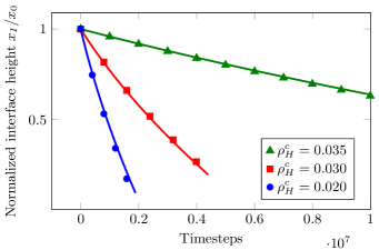
Figure 4: (Color online) Interface position as a function of time for different evaporation boundary densities $\rho^{c}_{H}=0.035$, $\rho^{c}_{H}=0.03$ and $\rho^{c}_{H}=0.02$. The theoretical prediction Eq. (22) (solid lines) agrees well with the simulation data (symbols)

With the assumption that the density profile across the interface is also linear, the total mass of fluid $c$ in the system is

$$M^{c}(t)=A\big{[}(x_{I}-d_{0})\rho^{c}_{ma}+(x_{H}-x_{I}-d_{0})$$

$$(\rho^{c}_{mi}+\rho^{c}_{H})/2+d_{0}(\rho^{c}_{ma}-\rho^{c}_{mi})\big{]}\mbox{,}$$ (17)

where $A$ is the area of the cross-section. From Eq. (17), we can obtain

$$dM^{c}/dt=A(\rho^{c}_{ma}-\rho^{c}_{mi}/2-\rho^{c}_{H}/2)\frac{dx_{I}}{dt}\mbox{.}$$ (18)

Based on the principle of mass conservation, the time evolution of mass obeys

$$M^{c}(t)=M^{c}(0)-A\int_{0}^{t}\mathbf{j}^{c}\cdot\mathbf{n}dt\mbox{,}$$ (19)

where $M^{c}(0)$ is the initial mass of fluid $c$. From Eq. (19), we can also get the time derivative of the total mass as

$$dM^{c}/dt=A|\mathbf{j}^{c}|\mbox{.}$$ (20)

By comparing Eq. (18) and Eq. (20), we obtain

$$\frac{dx_{I}}{dt}=\frac{D(\rho^{c}_{mi}-\rho^{c}_{H})}{(x_{H}-x_{I}-d_{0})(\rho^{c}_{ma}-\rho^{c}_{mi}/2-\rho^{c}_{H}/2)}.\,\,\,$$ (21)

We solve Eq. (21) with the initial condition $x_{I}(t=0)=x_{0}$ and finally obtain the interface position as a function of time

$$x_{I}(t)=x_{H}+d_{0}-\big{[}(x_{H}+d_{0}-x_{0})^{2}$$

$$+2\frac{D(\rho^{c}_{mi}-\rho^{c}_{H})}{\rho^{c}_{ma}-\rho^{c}_{mi}/2-\rho^{c}_{H}/2}t\big{]}^{1/2}.$$ (22)

The simulation results of the time evolution of the interface position for different evaporation boundary densities $\rho^{c}_{H}=0.035$, $\rho^{c}_{H}=0.03$ and $\rho^{c}_{H}=0.02$ along with our theoretical analysis Eq. (22) are presented in Fig. 4. We find excellent quantitative agreement between theory and simulation.

III.3 Evaporation of a freely suspended droplet

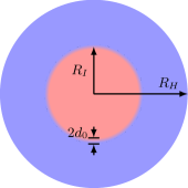
Figure 5: (Color online) Schematic cross-sectional representation of a droplet of radius $R_{I}$ surrounded by another fluid up to the spherical system boundary $R_{H}$, where the evaporation boundary condition is imposed.

In this section we investigate the evaporation of a freely floating droplet. A droplet of component $c$ with a radius of $R_{I}$ is the center of a spherical system of size $R_{H}$ and surrounded by component $\bar{c}$, as shown in Fig. 5. A spherical evaporation boundary is applied at $R_{H}$. Under the assumption of quasi-static dynamics, the density profile of component $c$ in the lighter phase satisfies the Laplace equation,

$$\Delta\mathbf{\rho}^{c}(r)=0\mbox{,}$$ (23)

where the boundary conditions are

$$\mathbf{\rho}^{c}(r)|_{r=R_{I}+d_{0}}=\rho^{c}_{mi}$$ (24)

and

$$\mathbf{\rho}^{c}(r)|_{r=R_{H}}=\rho_{H}^{c}\mbox{.}$$ (25)

In spherical coordinates, we obtain the analytical solution as

$$\!\!\mathbf{\rho}^{c}(r)=\rho_{H}^{c}-(\rho_{H}^{c}-\rho^{c}_{mi})\frac{R_{H}-r}{R_{H}-R_{I}-d_{0}}\frac{R_{I}+d_{0}}{r},\,\,$$ (26)

where $r$ is the distance from the center of a spherical coordinate system, originating at the droplet center. Inserting Eq. (26) into Eq. (13), we obtain the mass flux as

$$\mathbf{j}^{c}(r)=-D^{c}(\rho_{mi}-\rho^{c}_{H})\frac{R_{H}(R_{I}+d_{0})}{(R_{H}-R_{I}-d_{0})r^{2}}\mathbf{n}_{r},$$ (27)

where $\mathbf{n}_{r}$ is the normal vector to the droplet interface. Assuming the density profile across the interface also satisfies Laplace’s equation, we obtain the total mass of fluid $c$ in the system as

$$M^{c} = \int_{0}^{R_{I}-d_{0}}4\pi r^{2}\rho^{c}_{ma}dr+\int_{R_{I}-d_{0}}^{R_{I}+d_{0}}4\pi r^{2}\left(\rho^{c}_{mi}-(\rho^{c}_{mi}-\rho^{c}_{ma})\frac{R_{I}+d_{0}-r}{2d_{0}}\frac{R_{I}-d_{0}}{r}\right)dr$$ (28)

$$+\int_{R_{I}+d_{0}}^{R_{H}}4\pi r^{2}\left(\rho_{H}-(\rho_{H}-\rho^{c}_{mi})\frac{R_{H}-r}{R_{H}-R_{I}-d_{0}}\frac{R_{I}+d_{0}}{r}\right)dr\mbox{.}$$

We simplify Eq. (28) and derive the time derivative of the total mass as

$$dM^{c}/dt=\frac{2\pi}{3}\biggl{(}R_{H}^{2}\left(-\rho_{H}+\rho^{c}_{mi}\right)\\ +R_{H}\left(-2R_{I}\rho^{c}_{H}+2R_{I}\rho^{c}_{mi}-2d_{0}\rho^{c}_{H}+2d_{0}\rho^{c}_{mi}\right)\\ +6R_{I}^{2}\rho^{c}_{ma}-6R_{I}^{2}\rho^{c}_{mi}-2d_{0}^{2}\rho^{c}_{ma}+2d_{0}^{2}\rho^{c}_{mi}\biggr{)}dR_{I}/dt.$$ (29)

Based on the principle of mass conservation we have

$$M^{c}(t)=M^{c}(0)-\int_{0}^{t}4\pi r^{2}\mathbf{j}^{c}\cdot\mathbf{n}_{r}dt\mbox{,}$$ (30)

where $M^{c}(0)$ is the total initial mass of fluid $c$ in the system. From Eq. (30) with using Eq. (27), we also get the time derivative of the total mass as

$$dM^{c}/dt=4\pi D^{c}(\rho_{mi}-\rho^{c}_{H})\frac{(R_{I}+d_{0})R_{H}}{(R_{H}-R_{I}-d_{0})}\mbox{.}$$ (31)

By comparing Eq. (29) and Eq. (31) we obtain the time evolution of the droplet radius as

$$dR_{I}/dt=4\pi D^{c}(\rho_{mi}-\rho^{c}_{H})(R_{I}+d_{0})R_{H}\\ \bigg{[}(R_{H}-R_{I}-d_{0})\frac{2\pi}{3}\biggl{(}R_{H}^{2}\left(-\rho_{H}+\rho^{c}_{mi}\right)\\ +R_{H}\left(-2R_{I}\rho^{c}_{H}+2R_{I}\rho^{c}_{mi}-2d_{0}\rho^{c}_{H}+2d_{0}\rho^{c}_{mi}\right)\\ +6R_{I}^{2}\rho^{c}_{ma}-6R_{I}^{2}\rho^{c}_{mi}-2d_{0}^{2}\rho^{c}_{ma}+2d_{0}^{2}\rho^{c}_{mi}\biggr{)}\bigg{]}^{-1}\mbox{.}$$ (32)

We solve Eq. (32) numerically with a $4th$-order Runge-Kutta algorithm. For the simulations we initialize a droplet with a radius of $R_{0}=65$ and densities $\rho^{c}_{ma}=\rho^{\bar{c}}_{ma}=0.70$, $\rho^{c}_{mi}=\rho^{\bar{c}}_{mi}=0.04$, in a computational domain of $256^{3}$. The densities of fluid $c$ equilibrate to $\rho^{c}_{ma}\approx 0.712$ inside the droplet and $\rho^{c}_{mi}\approx 0.037$ outside. We initiate the evaporation by setting the density at the spherical evaporation boundary $r=R_{H}$ to $\rho^{c}_{H}=0.03$, $\rho^{c}_{H}=0.025$, and $\rho^{c}_{H}=0.02$. In Fig. 6 we compare the analytical solution Eq. (32) (dashed lines) with the simulation results (symbols). We note that Shan-Chen models are exposed to spurious vaporisation effects once the droplets become small, i.e. when the diameter is around $5-10$ lattice units.

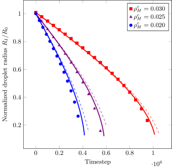
Figure 6: (Color online) Time evolution of the droplet radius for evaporation boundary densities $\rho^{c}_{H}=0.03$, $\rho^{c}_{H}=0.025$ and $\rho^{c}_{H}=0.02$. Our theoretical analysis without surface tension Eq. (32) (dashed lines) agrees quantitatively with the simulation data (symbols) for large droplet radii and deviates for small droplet radii. Our theoretical analysis which includes the surface tension Eq. (40) (solid lines) agrees quantitatively well with the simulation data for both large and small droplet radii.

To avoid the effect of the spurious vaporisation on the analysis, we only use the simulation data when the diameter of the droplet is larger than $20$ The analytical solution captures the qualitative features of the time evolution of the droplet radius well, and quantitatively agrees with the simulation data for the droplet at a larger radius. However, it deviates for small droplet radii. This can be explained by the fact that we neglected the effect of surface tension on the droplet evaporation. The surface tension induces a Laplace pressure, which is larger when the droplet radius becomes small EpsPle50 . We can take into account this effect as follows:

For a spherical droplet the Young-Laplace equation can be written as

$$P(r>R_{I},t)=P(r<R_{I},t)-\frac{2\gamma}{R_{I}},$$ (33)

where $\gamma$ is the surface tension, $P(r>R_{I},t)$ and $P(r<R_{I},t)$ are the pressures outside and inside the droplet at time $t$, respectively. We can write the pressure inside the droplet as Shan1993

$$P(r<R_{I},t)=c_{s}^{2}(\rho^{c}_{ma}+\rho^{\bar{c}}_{mi})+\frac{c_{s}^{2}}{2}g_{c\bar{c}}\Psi(\rho^{c}_{ma})\Psi(\rho^{\bar{c}}_{mi}).\,$$ (34)

For simplification, in the case of $\rho^{\bar{c}}_{mi}\ll\rho^{c}_{ma}$ we can write the pressure in terms of the leading term as

$$P(r<R_{I},t)=c_{s}^{2}\rho^{c}_{ma}.$$ (35)

The pressure outside the droplet can be treated as constant during evaporation, so that we get

$$P(r>R_{I},t) = P(r<R_{I},t=0)-\frac{2\gamma}{R_{0}}$$ (36)

$$= P(r<R_{I},t)-\frac{2\gamma}{R_{I}}.$$

By inserting Eq. (35) into Eq. (36), we obtain the majority density of fluid $c$ inside the droplet as

$$\rho^{c}_{ma}(t)=\rho^{c}_{ma}(t=0)-\frac{2\gamma}{c_{s}^{2}}\left(\frac{1}{R_{0}}-\frac{1}{R_{I}}\right).$$ (37)

The minority density of fluid $c$ outside the droplet can be treated as proportional to the majority density of fluid $c$ inside the droplet EpsPle50 . Thus we obtain

$$\!\!\!\!\!\rho^{c}_{mi}(t)=\rho^{c}_{mi}(t=0)\frac{\rho^{c}_{ma}(t=0)-\frac{2\gamma}{c_{s}^{2}}(\frac{1}{R_{0}}-\frac{1}{R_{I}})}{\rho^{c}_{ma}(t=0)}.\,\,\,$$ (38)

For brevity, we denote $\rho^{c}_{ma}(t=0)$ as $\rho^{c}_{ma,0}$ and $\rho^{c}_{mi}(t=0)$ as $\rho^{c}_{mi,0}$. We insert Eq. (37) and Eq. (38) into Eq. (28), and after some manipulations, we finally obtain the time derivative of the droplet mass as

$$dM^{c}/dt = \frac{2\pi}{3}\biggl{(}(-R_{H}^{2}-2R_{I}R_{H}-2R_{H}d_{0})\rho^{c}_{H}$$ (39)

$$+ (R_{H}^{2}+2R_{I}R_{H}+2R_{H}d_{0}-6R_{I}^{2}+2d^{2})\left(\rho^{c}_{mi,0}\frac{\rho^{c}_{ma,0}-\frac{2\gamma}{c_{s}^{2}}(\frac{1}{R_{0}}-\frac{1}{R_{I}})}{\rho^{c}_{ma,0}}\right)$$

$$+ (R_{I}R_{H}^{2}+dR_{H}^{2}+R_{I}^{2}R_{H}+2R_{I}R_{H}d_{0}+d_{0}^{2}R_{H}-2R_{I}^{3}+2R_{I}d^{2})\left(\frac{-2\gamma\rho^{c}_{mi,0}}{c_{s}^{2}\rho^{c}_{ma,0}}\frac{1}{R_{I}^{2}}\right)$$

$$+ (6R_{I}^{2}-2d^{2})(\rho^{c}_{ma,0}-\frac{2\gamma}{c_{s}^{2}}(\frac{1}{R_{0}}-\frac{1}{R_{I}}))+(2R_{I}^{3}-2R_{I}d^{2})(\frac{-2\gamma}{c_{s}^{2}R_{I}^{2}})\biggr{)}dR_{I}/dt.$$

We compare Eq. (39) with Eq. (31) and get the equation for $dR_{I}/dt$ including the effect of surface tension as

$$dR_{I}/dt = 4\pi D^{c}(\rho_{mi}-\rho^{c}_{H})(R_{I}+d_{0})R_{H}\bigg{[}(R_{H}-R_{I}-d_{0})\frac{2\pi}{3}\biggl{(}(-R_{H}^{2}-2R_{I}R_{H}-2R_{H}d_{0})\rho^{c}_{H}$$ (40)

$$+ (R_{H}^{2}+2R_{I}R_{H}+2R_{H}d_{0}-6R_{I}^{2}+2d^{2})\left(\rho^{c}_{mi,0}\frac{\rho^{c}_{ma,0}-\frac{2\gamma}{c_{s}^{2}}(\frac{1}{R_{0}}-\frac{1}{R_{I}})}{\rho^{c}_{ma,0}}\right)$$

$$+ (R_{I}R_{H}^{2}+dR_{H}^{2}+R_{I}^{2}R_{H}+2R_{I}R_{H}d_{0}+d_{0}^{2}R_{H}-2R_{I}^{3}+2R_{I}d^{2})\left(\frac{-2\gamma\rho^{c}_{mi,0}}{c_{s}^{2}\rho^{c}_{ma,0}}\frac{1}{R_{I}^{2}}\right)$$

$$+ (6R_{I}^{2}-2d^{2})(\rho^{c}_{ma,0}-\frac{2\gamma}{c_{s}^{2}}(\frac{1}{R_{0}}-\frac{1}{R_{I}}))+(2R_{I}^{3}-2R_{I}d^{2})(\frac{-2\gamma}{c_{s}^{2}R_{I}^{2}})\biggr{)}\bigg{]}^{-1}.$$

We solve Eq. (40) numerically and compare the theoretical prediction with simulation data in Fig. 6. The theoretical analysis including the effect of surface tension (solid lines) agrees quantitatively well with the simulation data (symbols) for both large and small droplet radii. Thus, we confirm that the effect of surface tension becomes significant when the droplets become small and must not be neglected. This result is of particular importance for lattice Boltzmann simulations of evaporating droplets since the typical number of lattice nodes available to resolve the radius of a single droplet is often limited. This holds in particular for systems involving a large number of droplets.

IV Conclusion

We presented a diffusion dominated evaporation model using the popular pseudopotential multicomponent lattice Boltzmann method introduced by Shan and Chen. The evaporation is induced by imposing the density of one component at the system boundary while ensuring total mass conservation, which causes diffusion of components driven by a density gradient. The diffusion coefficients depend on the densities of the fluids as well as the interaction strength parameters of the Shan-Chen model. With the analytically determined diffusion coefficients we confirm that the diffusion obeys Fick’s law.

We derived a theoretical model for the time evolution of the interface position of an evaporating planar film under the quasi-static assumption. Our theoretical model predicts that the evaporation flux is proportional to the density difference between the minority density and the evaporation boundary density $\rho_{mi}-\rho^{c}_{H}$, while the time evolution of the interface position obeys the expected $t^{0.5}$ law. We then carried out simulations which are in good quantitative agreement with our analytical model.

Furthermore, we derived analytical models describing the evaporation of a floating droplet surrounded by another fluid, as an extension of the famous Epstein-Plesset theory EpsPle50 . While the original publication assumes an infinite system, we extended the model towards a finite system size. We demonstrate a good agreement between theory and simulation if one takes into account the effect of surface tension causing a high Laplace pressure and an increased evaporation rate in the case of small droplet radii.

As an outlook we note that our method is not only suitable to simulate evaporating fluids, but that it is straightforward to apply it to investigate the condensation of droplets. Therefore, our method can be a powerful tool for exploring both evaporation and condensation processes in complex fluidic systems.

- (1) L. Wu, Z. Dong, M. Kuang, Y. Li, F. Li, L. Jiang, and Y. Song. Adv. Funct. Mater., 25:2237, 2015.
- (2) C. N. Kaplan, N. Wu, S. Mandre, J. Aizenberg, and L. Mahadevan. Phys. Fluids, 27:092105, 2015.
- (3) W. Han and Z. Lin. Angew. Chem. Int. Ed., 51:1534, 2011.
- (4) R. D. Deegan, O. Bakajin, T. F. Dupont, G. Huber, S. R. Nagel, and T. A. Witten. Nature, 389:827, 1997.
- (5) H. Gelderblom, A. G. Marín, H. Nair, A. van Houselt, L. Lefferts, J. H. Snoeijer, and D. Lohse. Phys. Rev. E, 83:026306, 2011.
- (6) P. S. Epstein and M. S. Plesset. J. Chem. Phys., 18:1505, 1950.
- (7) Y. O. Popov. Phys. Rev. E, 71:036313, 2005.
- (8) J. M. Stauber, S. K. Wilson, B. R. Duffy, and K. Sefiane. Langmuir, 31:3653, 2015.
- (9) A. G. Marín, H. Gelderblom, D. Lohse, and J. H. Snoeijer. Phys. Rev. Lett., 107:085502, 2011.
- (10) L. N. Long, M. M. Micci, and B. C. Wong. Comput. Phys. Commun., 96:167, 1996.
- (11) F. Wang and H. Wu. Soft Matter, 9:5703, 2013.
- (12) W. Chen, J. Koplik, and I. Kretzschmar. Phys. Rev. E, 87:052404, 2013.
- (13) D. Lohse and X. Zhang. Rev. Mod. Phys., 87:981, 2015.
- (14) S. Succi. The Lattice Boltzmann Equation: For Fluid Dynamics and Beyond. Oxford University Press, 2001.
- (15) R. Benzi, S. Succi, and M. Vergassola. Phys. Rep., 222:145, 1992.
- (16) D. Raabe. Modell. Simul. Mater. Sci. Eng., 12:R13, 2004.
- (17) H. Liu, Q. Kang, C. R. Leonardi, S. Schmieschek, A. Narváez, B. D. Jones, J. R. Williams, A. J. Valocchi, and J. Harting. Comput. Geosci., 20:777, 2016.
- (18) A. K. Gunstensen, D. H. Rothman, S. Zaleski, and G. Zanetti. Phys. Rev. A, 43:4320, 1991.
- (19) M. R. Swift, W. R. Osborn, and J. M. Yeomans. Phys. Rev. Lett., 75:830, 1995.
- (20) X. He, Sh. Chen, and R. Zhang. J. Comput. Phys., 663:642, 1999.
- (21) G. Falcucci, S. Ubertini, C. Biscarini, S. Di Francesco, D. Chiappini, S. Palpacelli, A. De Maio, and S. Succi. Commun. Comput. Phys., 9:269, 2011.
- (22) R. Ledesma-Aguilar, D. Vella, and J. M. Yeomans. Soft Matter, 10:8267, 2014.
- (23) G. Laghezza, E. Dietrich, J. M. Yeomans, R. Ledesma-Aguilar, E. S. Kooij, H. J. W. Zandvliet, and D. Lohse. Soft Matter, 12:5787, 2016.
- (24) H. P. Jansen, K. Sotthewes, J. van Swigchem, H. J. W. Zandvliet, and E. S. Kooij. Phys. Rev. E, 88:013008, 2013.
- (25) Q. Li, P. Zhou, and H. J. Yan. Langmuir, 32:9389, 2016.
- (26) A. S. Joshi and Y. Sun. Phys. Rev. E, 82:041401, 2010.
- (27) X. Shan and H. Chen. Phys. Rev. E, 47:1815, 1993.
- (28) N. Martys and H. Chen. Phys. Rev. E, 53:743, 1996.
- (29) J. Harting, C. Kunert, and H. J. Herrmann. Europhys. Lett., 75:328, 2006.
- (30) F. Jansen and J. Harting. Phys. Rev. E, 83:046707, 2011.
- (31) S. Frijters, F. Günther, and J. Harting. Soft Matter, 8:6542, 2012.
- (32) X. Shan and G. Doolen. Phys. Rev. E, 54:3614, 1996.
- (33) X. Shan and G. Doolen. J. Stat. Phys., 81:379, 1995.