Flux tubes in QCD with (2+1) HISQ fermions

Abstract:

We investigate the transverse profile of the chromoelectric field generated by a quark-antiquark pair in the vacuum of (2+1) flavor QCD. Monte Carlo simulations are performed adopting the HISQ/tree action discretization, as implemented in the publicly available MILC code, suitably modified to measure the chromoelectric field. We work on the line of constant physics, with physical strange quark mass $m_{s}$ and light to strange mass ratio $m_{l}/m_{s}=1/20$.

1 Introduction

Many fundamental questions are related to the large-scale behavior of Quantum ChromoDynamics (QCD). Remarkably, quarks and gluons appear to be confined in ordinary matter, due to the mechanism of color confinement which is not yet fully understood. A detailed understanding of color confinement is one of the central goals of nonperturbative studies of QCD. Lattice formulation of QCD allows us to investigate the color confinement phenomenon within a nonperturbative framework. It is known since long that, in lattice numerical simulations, tubelike structures emerge by analyzing the chromoelectric fields between static quarks [1, 2, 3, 4, 5, 6, 7, 8, 9]. Such tubelike structures naturally lead to a linear potential between static color charges and, consequently, to a direct numerical evidence of color confinement.
To explore on the lattice the field configurations produced by a static quark-antiquark pair, the following connected correlation function [1, 10] was used:

$$\rho_{W}^{\rm conn}=\frac{\left\langle{\rm tr}\left(WLU_{P}L^{\dagger}\right)\right\rangle}{\left\langle{\rm tr}(W)\right\rangle}-\frac{1}{N}\,\frac{\left\langle{\rm tr}(U_{P}){\rm tr}(W)\right\rangle}{\left\langle{\rm tr}(W)\right\rangle}\;,$$ (1)

where $U_{P}=U_{\mu\nu}(x)$ is the plaquette in the $(\mu,\nu)$ plane, connected to the Wilson loop $W$ by a Schwinger line $L$, and $N$ is the number of colors (see Fig. 1).

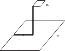
Figure 1: The connected correlator given in Eq. (1) between the plaquette $U_{P}$ and the Wilson loop (subtraction in $\rho_{W}^{\rm conn}$ not explicitly drawn).

The quark-antiquark field strength tensor is given by [1, 10]:

$$F_{\mu\nu}(x)=\sqrt{\frac{1}{g^{2}}}\,\rho_{W}^{\rm conn}(x)\;,$$ (2)

where $g$ is the gauge coupling. In previous studies [11, 4, 6, 7, 8, 12] color flux tubes made up of chromoelectric field directed along the line joining a static quark-antiquark pair have been investigated, in the cases of SU(2) and SU(3) pure gauge theories at zero temperature.
In this paper we study the profile of color flux tubes in pure SU(3) gauge theory and in QCD with (2+1) flavors and present some new preliminary results with sources at distances up to 1.14 fm.
The dual superconductor model [13, 14] of the QCD vacuum is, at least, a very useful phenomenological frame to interpret the vacuum dynamics and the formation of color flux tubes in the QCD vacuum. In Refs. [7, 8] it has been suggested that lattice data for chromoelectric flux tubes can be analyzed by exploiting the results presented in Ref. [15], where, from the assumption of a simple variational model for the magnitude of the normalized order parameter of an isolated vortex, an analytic expression is derived for magnetic field and supercurrent density, that solves the Ampere’s law and the Ginzburg-Landau equations. As a consequence, the transverse distribution of the chromoelectric flux tube can be described, according to [7, 8, 12], by

$$E_{l}(x_{t})=\frac{\phi}{2\pi}\frac{1}{\lambda\xi_{v}}\frac{K_{0}(R/\lambda)}{K_{1}(\xi_{v}/\lambda)}\;,\qquad R=\sqrt{x_{t}^{2}+\xi_{v}^{2}}$$ (3)

where $\xi_{v}$ is a variational core-radius parameter. Equation (3) can be rewritten as

$$E_{l}(x_{t})=\frac{\phi}{2\pi}\frac{\mu^{2}}{\alpha}\frac{K_{0}[(\mu^{2}x_{t}^{2}+\alpha^{2})^{1/2}]}{K_{1}[\alpha]}\;,\quad\mu=\frac{1}{\lambda}\,,\quad\frac{1}{\alpha}=\frac{\lambda}{\xi_{v}}\,.$$ (4)

By fitting Eq. (4) to flux-tube data, one can get both the penetration length $\lambda$ and the ratio of the penetration length to the variational core-radius parameter, $\lambda/\xi_{v}$. Moreover, the Ginzburg-Landau $\kappa$ parameter can be obtained by

$$\kappa=\frac{\lambda}{\xi}=\frac{\sqrt{2}}{\alpha}\left[1-K_{0}^{2}(\alpha)/K_{1}^{2}(\alpha)\right]^{1/2}\,.$$ (5)

Finally, the coherence length $\xi$ is determined by combining Eqs. (4) and (5).

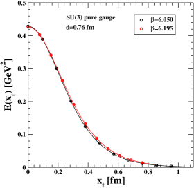
Figure 2: (left) SU(3) pure gauge: the chromoelectric field $E_{l}(x_{t})$ in physical units versus the transverse distance $x_{t}$ measured for two different values of the gauge coupling for a distance $d=0.76\,\,{\rm fm}$ between sources. Full lines are the fits using Eq. (4). (right) QCD (2+1) flavors: as for left figure.

2 Lattice setup and numerical results

Both for the cases of pure gauge SU(3) and QCD with (2+1) flavors we performed simulations on a $32^{4}$ lattice. We have made use of the publicly available MILC code [16], which has been suitably modified by us in order to introduce the relevant observables.

2.1 SU(3) pure gauge

Table 1: SU(3) pure gauge. The results of the fit to the chromoelectric field Eq. (4) at several distances $d$ between the sources, together with the square root width of the flux tube Eq. (8) and the square root of the energy in the flux tube per unit lenght normalized to the flux $\phi$, Eq. (9).

$\beta$	$d$ [fm]	$\phi$	$\lambda$ [fm]	$\kappa=\lambda/\xi$	$\xi$ [fm]	$\sqrt{w^{2}}$ [fm]	$\sqrt{\varepsilon}/\phi$ [GeV]
6.050	0.76	5.143(39)	0.164(5)	0.348(208)	0.472(283)	0.458(17)	0.133(5)
6.195	0.76	5.485(56)	0.173(7)	0.369(229)	0.469(293)	0.476(24)	0.128(7)
6.050	0.95	5.932(114)	0.169(16)	0.229(103)	0.738(339)	0.517(59)	0.116(14)
6.050	1.14	6.254(617)	0.166(95)	0.174(65)	0.953(651)	0.542(386)	0.109(82)

We measure on the lattice the chromoelectric field generated by a quark-antiquark pair at distances up to 1.14 fm. The scale is fixed using the parameterization [17]:

$$\left(a\,\sqrt{\sigma}\right)(g) = f_{{\rm{SU(3)}}}(g^{2})\left\{1+0.2731\,\hat{a}^{2}(g)\right.$$

$$- 0.01545\,\hat{a}^{4}(g)+0.01975\,\hat{a}^{6}(g)\left.\right\}/0.01364\;,$$

$$\hat{a}(g)=\frac{f_{{\rm{SU(3)}}}(g^{2})}{f_{{\rm{SU(3)}}}(g^{2}(\beta=6))}\;,\;\beta=\frac{6}{g^{2}}\,,\;\;\;5.6\leq\beta\leq 6.5\;,$$

with

$$f_{{\rm{SU(3)}}}(g^{2})=\left({b_{0}g^{2}}\right)^{-b_{1}/2b_{0}^{2}}\,\exp\left(-\frac{1}{2b_{0}g^{2}}\right)\;,\;\;\;b_{0}\,=\,\frac{11}{(4\pi)^{2}}\;\;,\;\;b_{1}\,=\,\frac{102}{(4\pi)^{4}}\,.$$ (7)

In the following, we assumed for the string tension the standard value of $\sqrt{\sigma}=420$ MeV.
We measured the connected correlator given in Eq. (1) at the middle of the line connecting the static color sources, for various values of the distance between the sources and for integer transverse distances. In order to reduce the ultraviolet noise, we applied to the operator in Eq. (1) one step of HYP smearing [18] to temporal links, with smearing parameters $(\alpha_{1},\alpha_{2},\alpha_{3})=(1.0,0.5,0.5)$, and $N_{\rm APE}$ steps of APE smearing [19] to spatial links, with smearing parameter $\alpha_{\rm APE}=0.40$. Here $\alpha_{\rm APE}$ is the ratio between the weight of one staple and the weight of the original link.

We fitted our data for the transverse shape of the longitudinal chromoelectric field to Eq. (4). Remarkably, we found that Eq. (4) is able to reproduce the transverse profile of the longitudinal chromoelectric field.

We checked that our lattice results are consistent with continuum scaling. To do this we measured the longitudinal chromoelectric field generated by sources at distance $8a$ and $10a$ (($a$ is the lattice spacing) for two values of the gauge couplings $\beta=6.050$ and $\beta=6.195$. According to the scale given in Eq. (2.1) this amounts to a distance of $0.76{\rm fm}$ in physical units. The result in Fig. 2 seems to display an almost perfect scaling. Having selected the gauge coupling region where continuum scaling holds, we measured the the longitudinal chromoelectric field at distances $10a$ and $12a$ at $\beta=6.050$ which corresponds respectively to distances $0.95{\rm fm}$ and $1.14{\rm fm}$ in physical units. In Fig. 3 we display the results. Now, using Eq. (4) and the values of the parameters obtained by fitting Eq. (4) to the numerical value for the longitudinal chromoelectric field, we are able to estimate the mean square root width of the flux tube:

$$\sqrt{w^{2}}=\sqrt{\frac{\int d^{2}x_{t}\,x_{t}^{2}E_{l}(x_{t})}{\int d^{2}x_{t}\,E_{l}(x_{t})}}=\sqrt{\frac{2\alpha}{\mu^{2}}\frac{K_{2}(\alpha)}{K_{1}(\alpha)}}$$ (8)

and the square root of the energy in the flux tube per unit length, normalized to the flux $\phi$:

$$\frac{\sqrt{\varepsilon}}{\phi}=\frac{1}{\phi}\sqrt{\int d^{2}x_{t}\,\frac{E_{l}(x_{t})^{2}}{2}}=\sqrt{\frac{\mu^{2}}{8\pi}\,\left(1-\left(\frac{K_{0}(\alpha)}{K_{1}(\alpha)}\right)^{2}\right)}$$ (9)

The results are given in Table 1. We can argue that the penetration length $\lambda$ is almost stable within errors at varying the distance between the sources. While there is a hint of slow increasing for $\xi$ and $\sqrt{w^{2}}$.

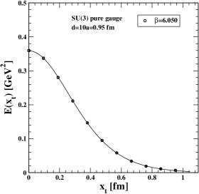
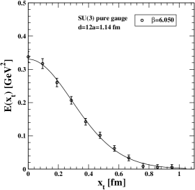
Figure 3: SU(3) pure gauge: the chromoelectric field $E_{l}(x_{t})$ in physical units versus the transverse distance $x_{t}$ measured for distance $d=0.95\,\,{\rm fm}$ (left) and distance $d=1.14\,\,{\rm fm}$ (right) between sources. Full lines are the fits using Eq. (4).

2.2 QCD (2+1) flavors

In this section we present results obtained for QCD with (2+1) flavors. Highly improved staggered quark action with tree level improved Symanzik gauge action (HISQ/tree) has been adopted (see ref.()). We work on the line of constant physics determined by fixing the strange quark mass to its physical value $m_{s}$ at each value of the gauge coupling. The light-quark mass has been fixed at $m_{l}=m_{s}/20$. This correspond to a pion mass $M_{\pi}=160\,\,{\rm MeV}$. The lattice spacing has been determined using results of Ref. [20]. As in the case of pure gauge SU(3) theory in order to measure the correlator Eq. (1) we perform one HYP smearing on temporal links and several APE smearings on spatial links. To check the continuum scaling we considered two different values of the gauge couplings $\beta=6.743$ and $\beta=6.885$ and measured the chromoelectric field produced by sources at distances $7a$ and $8a$ respectively. This amounts to have a distance of $0.76\,\,{\rm fm}$ between sources. The result displayed in Fig. 2 indicates a almost perfect scaling (see also Table 2 for the parameters obtained in fitting the data to Eq. (4). Then we measure the field produced for two other distances between the sources. Namely at gauge coupling $\beta=6.885$ we consider the distances $10a$ and $12a$ corresponding to $0.95\,\,{\rm fm}$ and $1.14\,\,{\rm fm}$. The results are displayed in Fig. 4. At variance with respect to the pure SU(3) gauge (see Fig. 3) the measurements for the chromoelectric field at distance $d=1.14\,{\rm fm}$ versus the the transverse distance seems to fluctuate around zero, although with large errors. This circumstance could suggest that, in presence of dynamical fermions and for a sufficiently large distance between sources, the flux tube structure disappears.

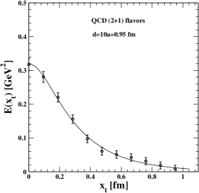
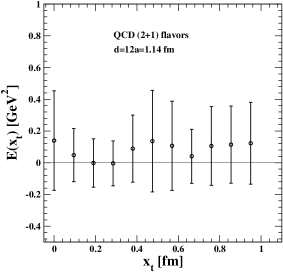
Figure 4: QCD (2+1) flavors: the chromoelectric field $E_{l}(x_{t})$ in physical units versus the transverse distance $x_{t}$ measured for distance $d=0.95\,\,{\rm fm}$ (left) and distance $d=1.14\,\,{\rm fm}$ (right) between sources. Full lines are the fits using Eq. (4).

Table 2: QCD (2+1) flavors. The results of the fit to the chromoelectric field Eq. (4) at several distances $d$ between the sources, together with the square root width of the flux tube Eq. (8) and the square root of the energy in the flux tube per unit lenght normalized to the flux $\phi$, Eq. (9).

$\beta$	$\Delta$ [fm]	$\phi$	$\lambda$ [fm]	$\kappa=\lambda/\xi$	$\xi$ [fm]	$\sqrt{w^{2}}$ [fm]	$\sqrt{\varepsilon}/\phi$ [GeV]
6.743	0.76	4.366(48)	0.139(8)	0.264(131)	0.526(263)	0.411(29)	0.146(11)
6.885	0.76	4.251(67)	0.147(10)	0.342(203)	0.429(256)	0.411(33)	0.148(13)

References

- [1] A. Di Giacomo, M. Maggiore, and S. Olejnik, Confinement and Chromoelectric Flux Tubes in Lattice QCD, Nucl. Phys. B347 (1990) 441–460.
- [2] P. Cea and L. Cosmai, Lattice investigation of dual superconductor mechanism of confinement, Nucl. Phys. Proc. Suppl. 30 (1993) 572–575.
- [3] Y. Matsubara, S. Ejiri, and T. Suzuki, The (dual) Meissner effect in SU(2) and SU(3) QCD, Nucl. Phys. Proc. Suppl. 34 (1994) 176–178, [hep-lat/9311061].
- [4] P. Cea and L. Cosmai, Dual superconductivity in the SU(2) pure gauge vacuum: A Lattice study, Phys. Rev. D52 (1995) 5152–5164, [hep-lat/9504008].
- [5] G. S. Bali, K. Schilling, and C. Schlichter, Observing long color flux tubes in SU(2) lattice gauge theory, Phys. Rev. D51 (1995) 5165–5198, [hep-lat/9409005].
- [6] M. S. Cardaci, P. Cea, L. Cosmai, R. Falcone, and A. Papa, Chromoelectric flux tubes in QCD, Phys.Rev. D83 (2011) 014502, [arXiv:1011.5803].
- [7] P. Cea, L. Cosmai, and A. Papa, Chromoelectric flux tubes and coherence length in QCD, Phys.Rev. D86 (2012) 054501, [arXiv:1208.1362].
- [8] P. Cea, L. Cosmai, F. Cuteri, and A. Papa, Flux tubes in the SU(3) vacuum: London penetration depth and coherence length, Phys. Rev. D89 (2014), no. 9 094505, [arXiv:1404.1172].
- [9] N. Cardoso, M. Cardoso, and P. Bicudo, Inside the SU(3) quark-antiquark QCD flux tube: screening versus quantum widening, Phys. Rev. D88 (2013) 054504, [arXiv:1302.3633].
- [10] D. S. Kuzmenko and Y. A. Simonov, Field distributions in heavy mesons and baryons, Phys. Lett. B494 (2000) 81–88, [hep-ph/0006192].
- [11] P. Cea and L. Cosmai, Dual Meissner effect and string tension in SU(2) lattice gauge theory, Phys. Lett. B349 (1995) 343–347, [hep-lat/9404017].
- [12] P. Cea, L. Cosmai, F. Cuteri, and A. Papa, Flux tubes at finite temperature, JHEP 06 (2016) 033, [arXiv:1511.01783].
- [13] G. ’t Hooft, The confinement phenomenon in quantum field theory, in High Energy Physics, EPS International Conference, Palermo, 1975 (A. Zichichi, ed.), 1975.
- [14] S. Mandelstam, Vortices and quark confinement in non Abelian gauge theories, Phys. Rept. 23 (1976) 245.
- [15] J. R. Clem, Simple model for the vortex core in a type ii superconductor, Journal of Low Temperature Physics 18 (1975) 427–434. 10.1007/BF00116134.
- [16] http://physics.utah.edu/~detar/milc.html.
- [17] R. G. Edwards, U. M. Heller, and T. R. Klassen, Accurate scale determinations for the Wilson gauge action, Nucl. Phys. B517 (1998) 377–392, [hep-lat/9711003].
- [18] A. Hasenfratz and F. Knechtli, Flavor symmetry and the static potential with hypercubic blocking, Phys. Rev. D64 (2001) 034504, [hep-lat/0103029].
- [19] M. Falcioni, M. Paciello, G. Parisi, and B. Taglienti, Again on su(3) glueball mass, Nuclear Physics B 251 (1985), no. 0 624 – 632.
- [20] A. Bazavov et al., The chiral and deconfinement aspects of the QCD transition, Phys. Rev. D85 (2012) 054503, [arXiv:1111.1710].