Heavy-traffic approximations for a layered network with limited resources

Abstract

Motivated by a web-server model, we present a queueing network consisting of two layers. The first layer incorporates the arrival of customers at a network of two single-server nodes. We assume that the inter-arrival and the service times have general distributions. Customers are served according to their arrival order at each node and after finishing their service they can re-enter at nodes several times (as new customers) for new services. At the second layer, active servers act as jobs which are served by a single server working at speed one in a Processor-Sharing fashion. We further assume that the degree of resource sharing is limited by choice, leading to a Limited Processor-Sharing discipline. Our main result is a diffusion approximation for the process describing the number of customers in the system. Assuming a single bottleneck node and studying the system as it approaches heavy traffic, we prove a state-space collapse property. The key to derive this property is to study the model at the second layer and to prove a diffusion limit theorem, which yields an explicit approximation for the customers in the system.

Keywords: Layered queueing network, limited processor sharing, fluid model, diffusion approximation, heavy traffic

1 Introduction

We consider a network with a two-layered architecture. The first layer models the processing of customers by a network of two nodes. Each node can have multiple (but finitely many) servers. Customers are served according to their order of arrival and after finishing their service, they can re-enter at nodes several times for new services. The servers of the first layer act as jobs in the second layer, where they are simultaneously served by a common server working at speed one according to Processor-Sharing (PS) with rates depending on the number of customers in the system. Our goal is to derive an explicit approximation of the process describing the number of customers in the system.

We analyze the system as it approaches heavy traffic. Under the assumption that there is a single bottleneck, we derive explicit results for the joint distribution of the number of customers in the system by proving a diffusion limit theorem. To achieve this, we look at the system in the second layer. In this way, we can aggregate the whole system since the total workload of the system (including the future workload due to customers re-entering the queues) acts as if were that of a single server queue with two independent renewal inputs.

To derive our diffusion limit theorem, we carry out a program inspired by the work of Barmson [1] and Williams [14], which consists of two main steps. First, we consider a critical fluid model, which can be thought of as a formal law of large numbers approximation under appropriate scaling. We identify the invariant states for the critical fluid model and we study the convergence to equilibrium of critical fluid model solutions as time goes to infinity. Our analysis has some similarities with the head-of-the-line processor sharing discipline as studied in [1], but there are differences. In particular, as the degree of resource sharing at each node is finite in our case, we need to define appropriate spatial regions in which the fluid model solutions have qualitatively different behavior. Our main result is to show that a solution of the fluid model converges to equilibrium uniformly (in terms of the initial condition) on compact sets. To achieve this, we perform a time change that facilitates our analysis.

The second main step is to show a state-space collapse property for the joint queue length vector process in heavy traffic. For an appropriately defined sequence of stochastic processes, we show that the difference between this vector and an appropriate deterministic mapping of the one-dimensional total workload process vanishes. The latter process is shown to converge to a one-dimensional reflected Brownian motion.

Our work can be seen as a partial network extension of the limited processor sharing (LPS) queue, of which fluid, diffusion, and steady-state heavy traffic limit theorems have been derived [18]–[20]. In our model, we assume that the inter-arrival and the service times have general distributions, but we consider that only one customer at each node can receive service at any time. In case that the inter-arrival and the service times are exponential, the service discipline at each station becomes irrelevant. An extension in the direction of general service times, using processor sharing at each node would require measure valued processes and is beyond the scope of the present paper. A mostly heuristic description of the results in this paper has appeared in [11]. In the classical applied probability literature, a version of our model has been investigated in a steady-state setting using boundary value techniques [6]; the solution in that paper may be used for numerical purposes, and is complementary to our heavy traffic limit, which yields explicit formulae, both for time-dependent as well as steady-state results.

In addition, our work is a contribution to the performance analysis of layered queueing networks. These are queueing networks where some entities in the system have a dual role (e.g., servers become customers to a higher-layer). In such systems, the dynamics in layers are correlated and the service speeds vary over time. Layered queueing networks can be characterised by separate layers (see [8] and [15]) or simultaneous layers. In the first case, customers receive service with some delay. An application where layered networks with separate layers appear is the manufacturing systems e.g., [3] and [4]. On the other hand, in layered networks with simultaneous layers, customers receive service from the different layers simultaneously. Layered networks with simultaneous layers have applications in communications networks. An application example where layered networks with simultaneous layers (such as our model) appear naturally are web-based multi-tiered system architectures. In such environments, different applications compete for access to shared infrastructure resources, both at the software level (e.g., mutex and database locks, thread-pools) and at the hardware level (e.g., bandwidth, processing power, disk access). For background, see [9] and [10].

The paper is organized as follows. We provide a detailed model description in Section 2 and we introduce the systems dynamics. In Section 3, we derive the fluid model and analyze it under the assumption of a single bottleneck and heavy traffic in the network. As we see, the assumption of the single bottleneck allows us to prove a State Space Collapse (SSC) property. Then, we show that a fluid model solution converges to equilibrium uniformly on compact sets. The main result of this paper is contained in Section 4. Namely, we provide a diffusion limit theorem for the joint customer population process for this two-layered queueing network. First, we prove that the diffusion scaled total workload process converges in distribution to a reflected Brownian motion. This result together with results in [1], lead to the main theorem..

2 Model

We assume a network with two layers. In layer 1, there are $2$ single-server nodes indexed by $i$. Customers arrive at node $i\in\{1,2\}$ randomly one by one and have a random service requirement. A customer completing service at node $i$ may be routed at node $l$, $l\in\{1,2\}$ for another service. It is assumed that customers are served according to their arrival order at each node; i.e., First In First Out. Only the first customer at each node can receive service at any time; i.e., the network is a Head of the Line network (HL).

In layer 2, there is a single server working at speed one. The servers of layer 1 are served by this single server simultaneously and at a rate which depends on the number of customers in the system. The model is illustrated in the following figure.

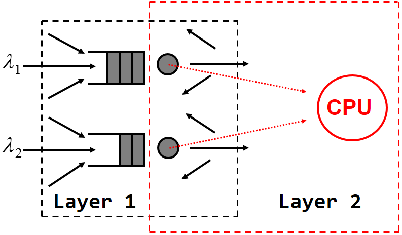
Figure 1: A two-layered network with $2$ single-server nodes and routing.

In Section 2.1, we give a formal description of the model and in Section 2.2, we introduce the dynamics describing the model. In the sequel, we use the subscript $i$ to refer to processes or quantities pertaining to each node and by convention, we omit the subscript to denote the 2-dimensional vector of these processes or quantities.

2.1 Preliminaries and model description

In this section, we give a formal model description. Let $(\Omega,\mathcal{F},\mathbb{P})$ be a probability space. For $T>0,$ let $\mathcal{D}[0,T]^{2}$ be the Skorokhod space; i.e., the space of 2-dimensional real-valued functions on $[0,T]$ that are right continuous with left limits endowed with the $J_{1}$ topology (as all candidate limit objects we consider are continuous, we actually only need to work with the uniform topology); cf. [2]. We denote by $\mathcal{B}(\mathcal{D}[0,T]^{2})$ the Borel $\sigma-$algebra of $\mathcal{D}[0,T]^{2}$. All the processes are defined from $(\Omega,\mathcal{F},\mathbb{P})$ to $(\mathcal{B}(\mathcal{D}[0,T]^{2}),\mathcal{D}[0,T]^{2}).$ For a process $X(t),$ we denote the uniform norm by $\|X(t)\|_{T}=\sup_{0\leq t\leq T}|X(t)|$, where $|X(\cdot)|=\max_{i}|X_{i}(\cdot)|.$ We adopt the convention that all mentioned vectors are 2-dimensional columns and use $a^{T}$ to denote the transpose of a vector or a matrix $a$. We use $A^{-1}$ to denote the inverse of a square matrix $A$, $A^{k}$ its $k^{\text{th}}$ power, and $\|A\|$ the maximum element of $A$. Furthermore, $I$ represents the identity matrix and $e$ and $e_{0}$ are the vectors consisting of 1’s and 0’s, respectively, the dimensions of which are clear from the context. Also, $e_{i}$ is the vector whose $i^{\text{th}}$ element is 1 and the rest are all 0. Last, for a real number $x$, its integer part is represented by $[x]$.

We start by describing the first layer. Let $u_{i}(j)$ for $j=2,3,\ldots$, be the time between the $(j-1)^{\text{th}}$ and $j^{\text{th}}$ external arrival at node $i$ and $u_{i}(1)>0$ be the residual arrival time of the first customer entering at node $i$ after time 0. We assume that the sequence $\{u_{i}(j)\}$ for $i=1,2$ and $j=2,3,\ldots$ is a sequence of positive i.i.d. random variables with mean $1/\lambda_{i}$, $\lambda_{i}>0,$ and that $u_{i}(1)$ is independent of this sequence but sampled from an arbitrary distribution with the same mean. For $i=1,2$, define the cumulative arrival time process $U_{i}(\cdot)$, as follows: $U_{i}(0)\mathrel{\mathop{\mathchar 58\relax}}=0$ and $U_{i}(m)\mathrel{\mathop{\mathchar 58\relax}}=\sum_{j=1}^{m}u_{i}(j)$ for $m\in\mathbb{N}$. The number of the external arrivals at node $i$ until time $t>0$ is given by the external arrival process

$$E_{i}(t)\mathrel{\mathop{\mathchar 58\relax}}=\max\{m\geq 0\mathrel{\mathop{\mathchar 58\relax}}U_{i}(m)\leq t\}.$$

In order to be able to define the total workload process in the system, including future service requirements due to routing, we need to introduce a sequence of random variables for any customer $j.$ For any fixed time $t\geq 0$ and $j>1$, let $v_{ii}^{(1)}(j),$ be the immediate service requirement of the $j^{\text{th}}$ customer (external or routed) at node $i.$ Also, we define $v_{il}^{(k+1)}(j)$ to be the service requirement of the $j^{\text{th}}$ customer (external or routed) at node $i$ at the $k^{\text{th}}$ future time he visits node $l,$ for $i,l\in\{1,2\}$ and $j,k\in\mathbb{N}.$ The sequence $\{v_{il}^{(k)}(j)\}$, indexed by $j$, is a sequence of i.i.d. random variables for any fixed $i,l,k$ and for $j>1$ and has mean $\beta_{l}\mathrel{\mathop{\mathchar 58\relax}}=1/\mu_{l},$ $\mu_{l}>0.$ The random variable $v_{ii}^{(1)}(1)$ denotes the residual service time for the first customer being served at node $i$ at time 0; it is independent of the sequence $\{v_{il}^{(k)}(j)\}$ but sampled from an arbitrary distribution with the same mean. In addition, we assume that all the above-mentioned random variables have finite second moments (more precisely, we need a Lindeberg-type condition to hold to make sure that the exogenous input processes satisfy a functional central limit theorem; see Section 4 for more details). We define the cumulative service time process as $V_{i}(0)\mathrel{\mathop{\mathchar 58\relax}}=0$ and for $m\in\mathbb{N}$,

$$V_{i}(m)\mathrel{\mathop{\mathchar 58\relax}}=\sum_{j=1}^{m}v_{ii}^{(1)}(j)\qquad i=1,2,$$

and the counting process

$$S_{i}(t)\mathrel{\mathop{\mathchar 58\relax}}=\max\{m\geq 0\mathrel{\mathop{\mathchar 58\relax}}V_{i}(m)\leq t\}.$$ (2.1)

We shall use the random variables $\{v_{il}^{(k+1)}(j)\}$ to count the future workload in the system at time $t$. For a fixed $t>0$, $v_{il}^{(k+1)}(j)$ represents the $k^{\text{th}}$ future service requirement of the $j^{\text{th}}$ customer waiting to being served at node $i$ and routed at node $l.$ This event will occur after time $t$ and after the completion of his service at node $i.$

Customers can move between queues according to Markovian routing. To describe the routing process, we define the following quantities. Let $P$ be the (square) routing matrix of dimension $2$. It is assumed that it is substochastic with a spectral radius less than one; i.e., its largest eigenvalue is less than one. In other words, the network is open, so the following relations hold:

$(I-P^{T})^{-1}=I+\sum_{k=1}^{\infty}(P^{T})^{k}$ and $\lim_{k\rightarrow\infty}(P^{T})^{k}=0.$

For any customer $j$ at node $i$ (external or routed), we define the random variables $\varphi^{(k)}_{il}(j)=1$ if the $j^{\text{th}}$ departing customer from node $i$ is routed to node $l$ in $k$ steps. The probability of this event is given by

$$\mathbb{P}(\varphi^{(k)}_{il}(j)=1)=p^{(k)}_{il},$$

where $p^{(k)}_{il}$ denotes the $(i,l)^{\text{th}}$ element of the matrix $P^{k}$. For $i=1,2$, we define the 2-dimensional random vector

$$\varphi^{(k)}_{i}(j)\mathrel{\mathop{\mathchar 58\relax}}=(\varphi^{(k)}_{i1}(j),\varphi^{(k)}_{i2}(j))^{T}.$$

Note that $\varphi^{(k)}_{i}(j)$ can take values in the set $\{e_{0},e_{1},e_{2}\}$, where $\varphi^{(k)}_{i}(j)=e_{0}$ means that the $j^{\text{th}}$ customer leaves the system. Let $\bar{p}^{(k)}_{i}$ be the $i^{\text{th}}$ column of the matrix $(P^{T})^{k}$. The expectation and the covariance matrix of $\varphi^{(k)}_{i}(j),$ for $i=1,2,$ are given by

$\mathbb{E}(\varphi^{(k)}_{i}(j))=\bar{p}^{(k)}_{i}$  and $\mathbb{C}(\varphi^{(k)}_{i}(j))=\begin{bmatrix}p^{(k)}_{i1}(1-p^{(k)}_{i2})&-p^{(k)}_{i1}p^{(k)}_{i2}\\ -p^{(k)}_{i1}p^{(k)}_{i2}&p^{(k)}_{i2}(1-p^{(k)}_{i1})\end{bmatrix}.$

Now, we can define the routing process, which counts the number of customers who are routed from node $l$ to node $i$ as

$$\Phi_{li}(m)\mathrel{\mathop{\mathchar 58\relax}}=\sum_{j=1}^{m}\varphi_{li}^{(1)}(j),\quad i,l=1,2,\ m\in\mathbb{N}.$$

The total arrival rate at node $i$, $\gamma_{i}$, is given by the solution of the following traffic equations

$$\gamma_{i}=\lambda_{i}+\sum_{l=1}^{2}p_{li}^{(1)}\gamma_{l},\ i=1,2.$$

In vector form, this can be written as

$$\gamma=(I-P^{T})^{-1}\lambda.$$ (2.2)

It is shown in [2, Theorem 7.3] that under the assumptions described above, (2.2) has a unique solution $\gamma=(\gamma_{1},\gamma_{2})^{T}$. The traffic intensity of node $i$ is $\rho_{i}\mathrel{\mathop{\mathchar 58\relax}}=\gamma_{i}/\mu_{i}.$

Now, we describe the service discipline at the second layer. Here, there is a single server. The servers of layer 1 become jobs at layer 2 in the sense they are served by the server of layer 2 simultaneously and at a rate that depends on the number of customers in layer 1 (at any time). The rate that each node receives is given by the service allocation function $R(\cdot)\mathrel{\mathop{\mathchar 58\relax}}\mathbb{R}_{+}^{2}\rightarrow\mathbb{R}_{+}^{2}$, with $R(\cdot)\mathrel{\mathop{\mathchar 58\relax}}=(R_{1}(\cdot),R_{2}(\cdot))^{T}$ and for $i=1,2,$

$$R_{i}(q)\mathrel{\mathop{\mathchar 58\relax}}=\left\{\begin{array}[]{ll}\frac{\min\{{q_{i}},{K_{i}}\}}{\sum_{j=1}^{2}\min\{{q_{j}},{K_{j}}\}}&\mbox{if }q_{i}\neq 0,\\ 0&\mbox{if }q_{i}=0.\end{array}\right.$$ (2.3)

The quantity $q_{i}$ represents the number of customers at node $i.$ The $2$-dimensional vector $K=(K_{1},K_{2})^{T}$ is constant and we call it the degree of resource sharing. We assume that it is always finite and the user can choose it as a parameter of the system. Observe that $K$ in this service allocation function guarantees a minimum service rate for each customer in the system. Also, note that the above function is Lipschitz continuous for $q\neq(0,0).$

We make the additional assumption that there exists a unique bottleneck in our system, which w.l.o.g. we let it be node 1. The definition of bottleneck is given below.

Definition 2.1 (Bottleneck).

Node $i$ is a bottleneck if $i=\arg\min_{j}\frac{\mu_{j}K_{j}}{\gamma_{j}},\ j=1,2.$

By the previous definition, a straightforward inequality follows

$$\frac{\rho_{1}}{K_{1}}>\frac{\rho_{2}}{K_{2}}.$$ (2.4)

Observe that, if $K_{1}=K_{2},$ an intuitive explanation of the above definition is that the average occupancy of the server at node 1 is strictly greater than the server at node 2. In case of multi-server nodes where $K_{i}$ represents the number of servers an node $i,$ the fraction $\frac{\rho_{i}}{K_{i}}$ is the average occupancy of a server at node $i.$

2.2 System dynamics

In this section, we introduce the dynamics that describe our model. We denote by $Q_{i}(t)$ the number of customers at node $i$ at time $t$. This is given by

$$Q_{i}(t)=Q_{i}(0)+E_{i}(t)+\sum_{l=1}^{2}\Phi_{li}\Big{(}S_{l}\big{(}T_{l}(t)\big{)}\Big{)}-S_{i}\big{(}T_{i}(t)\big{)},$$ (2.5)

where $Q_{i}(0)$ denotes the number of customers initially at node $i.$ We define the cumulative service time of the server at node $i$ as

$$T_{i}(t)=\int_{0}^{t}R_{i}(Q(s))ds.$$ (2.6)

This quantity can be viewed as the effort that the server of node $i$ has put in processing customers during $[0,t].$ Note that as the allocation function might be less than one, the above process is not necessarily equal to the amount of time that the server at node $i$ is busy during $[0,t].$ In case the other node is empty during $[0,t],$ (2.6) coincides with the busy time at node $i$. Recall that $E_{i}(t)$ is the number of external arrivals at node $i$ up to time $t.$ Observe that $S_{i}\big{(}T_{i}(t)\big{)},$ which is a composition of the renewal process (2.1) and the process $T_{i}(t)$, represents the number of departures at node $i$ until time $t$. Furthermore, the total arrival process is given by

$$A_{i}(t)=E_{i}(t)+\sum_{l=1}^{2}\Phi_{li}\Big{(}S_{l}(T_{l}(t))\Big{)}.$$ (2.7)

The amount of time that both servers at the nodes are idle during $[0,t]$ is given by the 1-dimensional process

$$Y_{L_{2}}(t)=t-\sum_{i=1}^{2}T_{i}(t).$$ (2.8)

Alternatively, we can see this quantity as the idle time of the server in layer 2 during $[0,t]$. Further, the immediate workload at node $i$ at time $t$ is defined as

$$W_{i}(t)=V_{i}\Big{(}Q_{i}(0)+A_{i}(t)\Big{)}-T_{i}(t).$$ (2.9)

Observe that $W_{i}(t)$ is nonnegative for any $t\geq 0$. Last, due to the work-conserving property in layer 2, the following relation holds:

$$Y_{L_{2}}(t)\textrm{ increases }\Rightarrow W_{1}(t)+W_{2}(t)=0,\qquad t\geq 0,\ i=1,2.$$ (2.10)

Recall that when we omit the subscript $i$, we refer to the 2-dimensional column vector of the corresponding process/quantity; for example $A(\cdot)=(A_{1}(\cdot),A_{2}(\cdot))^{T}$ and $W(\cdot)=(W_{1}(\cdot),W_{2}(\cdot))^{T}.$ All the essential information of the evolution of the system is contained is the following 6-tuple

$$\mathfrak{X}(\cdot)\mathrel{\mathop{\mathchar 58\relax}}=(A(\cdot),S(\cdot),Q(\cdot),T(\cdot),Y_{L_{2}}(\cdot),W(\cdot)).$$

In addition, the total (immediate and future) workload of the system plays a key role in our analysis. First, we define the remaining service requirement of the $j^{\text{th}}$ customer waiting to be served at node $i=1,2$ as

$$s_{i}(j)\mathrel{\mathop{\mathchar 58\relax}}=v_{ii}^{(1)}(j)+s^{\prime}_{i}(j),$$ (2.11)

where

$$s^{\prime}_{i}(j)\mathrel{\mathop{\mathchar 58\relax}}=\sum_{l=1}^{2}\sum_{k=1}^{\infty}\varphi^{(k)}_{il}(j)v_{il}^{(k+1)}(j)$$

is the future service requirement of the above-mentioned customer. Observe that, for an external arrival, $s_{i}(j)$ is the total service requirement. The first and the second moments of (2.11) are given (in vector form) by

$$\tau\mathrel{\mathop{\mathchar 58\relax}}=\mathbb{E}(s(j))=(I-P)^{-1}\beta$$ (2.12)

and

$$\tau^{(2)}\mathrel{\mathop{\mathchar 58\relax}}=\mathbb{E}(s^{2}(j))=(I-P)^{-1}(\mathbb{E}(v^{2}(j))+2\beta(P\tau)).$$ (2.13)

Now, we can define the (1-dimensional) total workload of the system as

$$W_{Tot}(t)\mathrel{\mathop{\mathchar 58\relax}}=\sum_{i=1}^{2}W_{i}(t)+\sum_{i=1}^{2}\sum_{j=S_{i}\big{(}T_{i}(t)\big{)}+1}^{Q_{i}(0)+A_{i}(t)}s^{\prime}_{i}(j).$$ (2.14)

In case that $S_{i}\big{(}T_{i}(t)\big{)}=Q_{i}(0)+A_{i}(t)$, i.e., there are no customers at node $i$, we understand the second sum of the last equation as zero. Obviously, the total workload is not a Markov process as it is dependent on future service requirements. In Section 4.1, we shall see that under an appropriate scaling (i.e., the diffusion scaling) the dependence of the total workload on the future vanishes.

Last, as our network is HL, only one customer can be in service at node $i$ at any time. This property gives an upper and a lower bound for the cumulative service time (2.6) at node $i,$ which is given in [1, Inequality 2.13]; namely

$$V_{i}(S_{i}(T_{i}(t)))\leq T_{i}(t)<V_{i}(S_{i}(T_{i}(t))+1).$$ (2.15)

We have so far defined the system dynamics for the above-mentioned two layered network and stated all the assumptions we need for our analysis. We are now ready to study the fluid model of this network, which is the first essential step to show a SSC property.

3 Fluid analysis

In this section, we study a critical fluid model, which is a deterministic model and can be thought of as a formal law of large numbers approximation under appropriate scaling. We shall give a rigorous proof of the last statement in the next section.

The main goal is to prove uniform convergence (w.r.t. the initial condition) on compact sets for the fluid model under the critical loading assumption; i.e., the traffic intensity of the network is one. First, we find the invariant points (or equilibrium states) and define an appropriate lifting map which describes these points. Then, we define a time-changed version of the original fluid model and we show that it is enough to prove the convergence for the time-changed function. As the time-changed function is given by a piece-wise linear ODE, we are able to find the solution and to show the convergence. Because the degree of resource sharing (the vector $K$) is finite we need to separate the state space in suitable regions and to distinguish cases depending on initial conditions.

3.1 Definition and invariant points

The traffic intensity of the network is given by $\rho\mathrel{\mathop{\mathchar 58\relax}}=\beta^{T}\gamma=\sum_{i=1}^{2}\rho_{i}.$ We make the critical loading assumption, i.e.,

$$\rho=\rho_{1}+\rho_{2}=1.$$ (3.1)

To derive the fluid model equations we replace any random quantity in (2.5)–(2.10) with its mean. The fluid model equations are given by

$$\bar{Q}_{i}(t)=\bar{Q}_{i}(0)+\lambda_{i}t+\sum_{l=1}^{2}p_{li}\mu_{l}\bar{T}_{l}(t)-\mu_{i}\bar{T}_{i}(t),$$ (3.2)

$$\bar{T}_{i}(t)=\int_{0}^{t}R_{i}(\bar{Q}(s))ds,$$ (3.3)

$$\sum_{i=1}^{2}\bar{T}_{i}(t)+\bar{Y}_{L_{2}}(t)=t,$$ (3.4)

$$\bar{W}_{i}(t)=\beta_{i}\Big{(}\lambda_{i}t+\sum_{l=1}^{2}p_{li}\mu_{l}\bar{T}_{l}(t)+\bar{Q}_{i}(0)\Big{)}-\bar{T}_{i}(t),$$ (3.5)

$$\bar{Y}_{L_{2}}(t)\textrm{ increases }\Rightarrow\bar{W}_{1}(t)+\bar{W}_{2}(t)=0,\qquad t\geq 0,\ i=1,2.$$ (3.6)

We can show that the immediate workload in the fluid model can be written as $\bar{W}_{i}(t)=\beta_{i}\bar{Q}_{i}(t).$

Definition 3.1 (Fluid model).

We say that a $2$-dimensional vector $\bar{Q}(\cdot)$ with non-negative components is a solution of the fluid model if it is continuous and satisfies (3.2)–(3.6) for $t\in[0,\delta)$, and $Q(t)=0$ for $t\geq\delta$, with $\delta=\inf\{t\mathrel{\mathop{\mathchar 58\relax}}Q(t)=0\}$.

We define an auxiliary quantity, which can be interpreted as the total workload in the fluid model. It is defined by function $\bar{Q}(\cdot)$ as follows:

$$\begin{split}\bar{W}_{Tot}(t)=\beta^{T}\bar{Q}(t)+\sum_{k=1}^{\infty}\sum_{i=1}^{2}\beta^{T}\bar{p}^{(k)}_{i}\bar{Q}_{i}(t)&=\beta^{T}\bar{Q}(t)+\sum_{k=1}^{\infty}\beta^{T}(P^{T})^{k}\bar{Q}(t)\\ &=\beta^{T}(I-P^{T})^{-1}\bar{Q}(t)=\tau^{T}\bar{Q}(t).\end{split}$$

A useful result in our analysis is that the fluid total workload in the system remains constant under the critical loading assumption.

Proposition 3.1.

For any fluid model solution $\bar{Q}(\cdot)$, we have that

$$\bar{W}_{Tot}(t)=\beta^{T}(I-P^{T})^{-1}\bar{Q}(t)=\bar{W}_{Tot}(0).$$

Proof.

If $\bar{Q}(0)=0,$ then $\bar{W}_{Tot}(t)\equiv 0,$ for $t\geq 0.$ Let $\bar{Q}(0)>0.$ Assume now $\bar{Q}(0)=0$. By definition, $\bar{Q}(t)$ is continuous, so let $t$ be such that $\bar{Q}(t)$ is positive in a neighborhood of $t$. Calculating the derivative of the total workload at time $t$, we derive

$$\begin{split}\bar{W}_{Tot}^{\prime}(t)=&\beta^{T}(I-P^{T})^{-1}\bar{Q}^{\prime}(t)=\beta^{T}(I-P^{T})^{-1}(\lambda-(I-P^{T})(\mu\circ R(\bar{Q}(t))\\ =&\beta^{T}\gamma-\beta^{T}(\mu\circ R(\bar{Q}(t)))=\beta^{T}\gamma-\sum_{i=1}^{2}R_{i}(\bar{Q}(t))=0.\end{split}$$

The last equation holds due to (3.1) and the property of the service allocation function; i.e. $\sum_{i=1}^{2}R_{i}(\bar{Q}(t))=1.$ It follows that $\bar{W}_{Tot}(t)=\bar{W}_{Tot}(0)$ for $t\geq 0.$ Thus, $\bar{W}_{Tot}(t)$ is constant on $[0,\delta]$. Combining this with the continuity of $\bar{Q}(t)$, we see that, necessarily, $\delta=\infty$. Thus, the result extends to all positive $t$. ∎

In the following lemma, we show that there exists a solution to the fluid model equations for all non-zero initial states and it is unique.

Lemma 3.2 (Existence and uniqueness).

For any $\bar{Q}(0)\in\mathbb{R}_{+}^{2}\backslash\{0\}$ there exists a unique solution to the fluid model equations.

Proof.

Let $\bar{Q}(0)>0$. A by-product of the previous lemma is that $\delta=\infty$. Thus, we can discard the origin and define the function $\Psi(\cdot)\mathrel{\mathop{\mathchar 58\relax}}\mathbb{R}_{+}^{2}\backslash\{0\}\rightarrow\mathbb{R}_{+}^{2}$ as

$$\Psi(\cdot)\mathrel{\mathop{\mathchar 58\relax}}=\lambda-(I-P^{T})(\mu\circ R(\cdot)),$$ (3.7)

where $\mu\circ R(\cdot)$ indicates the Hadamard product; i.e., $\mu\circ R(\cdot)=(\mu_{1}R_{1}(\cdot),\mu_{2}R_{2}(\cdot))^{T}$. This function is Lipschitz continuous because $R(\cdot)$ is. Now, note that (3.2) can be written as

$$\bar{Q}^{\prime}(t)=\Psi(\bar{Q}(t)),\quad t\geq 0,$$ (3.8)

where the prime denotes the derivative with respect to time. The existence and uniqueness follows directly by [12, Section 10, Theorem IV]. ∎

Now, we characterize the invariant points $x\in\mathbb{R}^{2}_{+}$ of the fluid model. Before we state our result, we first proceed in an informal manner. Equate the total rate into node $i$ with the total rate out of node $i$. That is,

$$\gamma_{i}=\mu_{i}R_{i}(x).$$ (3.9)

Thus, we have that for the points on the invariant manifold (i.e. the set of the invariant points), $\rho_{i}=R_{i}(x)$. Using the definition of a bottleneck and keeping in mind that we assume node 1 to be the bottleneck, we now describe the invariant points. We know by (2.4) that $\frac{\rho_{1}}{K_{1}}>\frac{\rho_{2}}{K_{2}}$, which yields

$$\frac{K_{1}}{K_{2}}<\frac{\rho_{1}}{\rho_{2}}=\frac{R_{1}(x)}{R_{2}(x)}.$$

Thus, by combining the last inequality and the definition of the service allocation function (2.3), we have that the following inequality holds

$$\min\{{x_{2}},{K_{2}}\}<\frac{K_{2}}{K_{1}}\min\{{x_{1}},{K_{1}}\}\leq K_{2}.$$

The last inequality implies that for all invariant points $x=(x_{1},x_{2})$ of the fluid model, we have that $x_{2}<K_{2}.$ Thus, solving (3.9) for $x_{2}$ now yields $x_{2}=\frac{\rho_{2}}{\rho_{1}}\min\{{x_{1}},{K_{1}}\}.$ The invariant manifold is thus given by

$$\mathcal{I}=\bigg{\{}x\in\mathbb{R}^{2}_{+}\mathrel{\mathop{\mathchar 58\relax}}x_{2}=\frac{\mu_{1}}{\gamma_{1}}\frac{\gamma_{2}}{\mu_{2}}\min\{{x_{1}},{K_{1}}\}\bigg{\}}.$$ (3.10)

We make the previous arguments rigorous by showing that a sufficient and necessary condition of the fluid queue length to remain constant in time is the initial state lies on the invariant manifold.

Proposition 3.3.

Let $\bar{Q}(t)$ be a solution of (3.8). Then, $\bar{Q}(t)=\bar{Q}(0)$ for all $t\geq 0$ if and only if $\bar{Q}(0)\in\mathcal{I}.$

Proof.

The definition of the invariant manifold of an ODE is the set of all initial states such that the function remains constant; i.e., $\{\bar{Q}(0)\in\mathbb{R}^{2}_{+}\mathrel{\mathop{\mathchar 58\relax}}\bar{Q}(t)=\bar{Q}(0),t\geq 0\}$. Suppose now that $\bar{Q}(0)\in\mathcal{I}$. In this case, by the definition of an invariant point, $\bar{Q}(t)$ should be constant. So, $\bar{Q}(t)=\bar{Q}(0)\in\mathcal{I}.$

Now, supposing that $\bar{Q}(t)=\bar{Q}(0)\in\mathbb{R}_{+}^{2}$ for all $t\geq 0,$ then it follows from the previous discussion that $\bar{Q}(0)\in\mathcal{I}$.

∎

Having found the invariant (or equilibrium) points of the fluid model, we now turn to its stability property, namely the convergence of the solutions of fluid model equations to the invariant manifold as time goes to infinity.

3.2 Convergence to the invariant manifold for the fluid model

Let $x^{\ast}$ be the critical point in the invariant manifold where $x_{1}^{\ast}=K_{1}$, which means that $x^{\ast}_{2}=\frac{\mu_{1}}{\gamma_{1}}\frac{\gamma_{2}}{\mu_{2}}K_{1}$. For this point, we define the critical workload as (cf. (3.1))

$$w^{\ast}\mathrel{\mathop{\mathchar 58\relax}}=\beta^{T}(I-P^{T})^{-1}x^{\ast}=\tau^{T}x^{\ast}.$$ (3.11)

In order to prove a SSC property based on the critical workload level $w^{\ast},$ we define a lifting map, $\Delta\mathrel{\mathop{\mathchar 58\relax}}\mathbb{R}_{+}\rightarrow\mathbb{R}_{+}^{2},$ as follows:

$$\Delta_{1}(w) \mathrel{\mathop{\mathchar 58\relax}}=\frac{\min\{w,w^{\ast}\}}{w^{\ast}}K_{1}+\frac{\max\{w-w^{\ast},0\}}{\tau_{1}},$$ (3.12)

$$\Delta_{2}(w) \mathrel{\mathop{\mathchar 58\relax}}=\frac{\min\{w,w^{\ast}\}}{w^{\ast}}\frac{\rho_{2}K_{1}}{\rho_{1}}.$$

Note that the lifting map is Lipschitz continuous with constant $C_{1}=\max\{2\frac{K_{1}}{w^{\ast}}+\mu_{1},2C_{2}\}$ where $C_{2}=\frac{\mu_{1}K_{1}}{\lambda_{1}w^{\ast}}\max_{i}\frac{\lambda_{i}}{\mu_{i}}$. In the sequel, we show that fluid model solution converges to the invariant manifold as $t$ goes to infinity.

Theorem 3.4 (Convergence to the invariant manifold for the fluid model).

If $\bar{Q}(0)=(\bar{Q}_{1}(0),\bar{Q}_{2}(0))\in[0,M]^{2}$ for some $M>0,$ then for any $\epsilon>0,$ there exists a $t_{0}\geq 0$ (independent of $M$) such that

$$\sup_{\bar{Q}(0)\in[0,M]^{2}}|\bar{Q}(t)-\Delta\bar{W}_{Tot}(0)|\leq\epsilon,$$ (3.13)

for $t>t_{0}$ and $\Delta\bar{W}_{Tot}(0)$ is an invariant state.

Sketch of proof.

Here, we give a sketch of the proof. The complete proof is extended in the rest of this section. The first step is to define a function $y(\cdot)$ and a function $G(\cdot),$ and to show that $y(\cdot)$ can be interpreted as a time-change of $\bar{Q}(t),$ namely $\bar{Q}(t)=y(G(t)).$ Then, we show that the convergence of the time changed version implies the convergence of the original function $\bar{Q}(\cdot).$ To this end, let $\Xi=\{\xi_{ij}\}$, $i,j\in\{1,2\}$ be the matrix

$$\Xi=\begin{bmatrix}\lambda_{1}+\mu_{1}p_{11}-\mu_{1}&\lambda_{1}+\mu_{2}p_{21}\\ \lambda_{2}+\mu_{1}p_{12}&\lambda_{2}+\mu_{2}p_{22}-\mu_{2}\end{bmatrix}.$$

Define a function $y(\cdot)\mathrel{\mathop{\mathchar 58\relax}}[0,\infty)\rightarrow[0,\infty)^{2}$ such that $y_{i}(0)=\bar{Q}_{i}(0)$ and

$$y^{\prime}(t)=\Xi\Big{(}\min\{y_{1}(t),K_{1}\},\min\{y_{2}(t),K_{2}\}\Big{)}^{T}.$$ (3.14)

We shall show that the above-defined function can be interpreted as a time-change of $\bar{Q}(t).$ Let $G(\cdot)\mathrel{\mathop{\mathchar 58\relax}}[0,\infty)\rightarrow[0,\infty)$ be the solution of

$$G^{\prime}(t)=\frac{1}{\sum_{i=1}^{2}\min\{y_{i}(G(t)),K_{i}\}}.$$

Note that $G(\cdot)$ is continuous and that

$$G(t)=\int_{0}^{t}\frac{1}{\sum_{i=1}^{2}\min\{y_{i}(G(s)),K_{i}\}}ds\geq\frac{1}{\sum_{i=1}^{2}K_{i}}t.$$

This means that the function $G(\cdot)$ is strictly increasing and unbounded in time, which implies that $G(\cdot)$ is also invertible. The original function $\bar{Q}(t)$ can be interpreted as $\bar{Q}_{i}(t)=y_{i}(G(t)),$ for $t>0.$ To see this,

$$\begin{split}\bar{Q}^{\prime}(t)=y^{\prime}(G(t))G^{\prime}(t)&=\Xi\Big{(}\min\{y_{1}(G(t)),K_{1}\},\min\{y_{2}(G(t)),K_{2}\}\Big{)}^{T}\frac{1}{\sum_{i=1}^{2}\min\{y_{i}(G(t)),K_{i}\}}\\ &=\Xi\Big{(}R_{1}(\bar{Q}(t)),R_{2}(\bar{Q}(t))\Big{)}^{T}=\Psi(\bar{Q}(t)),\end{split}$$

where the function $\Psi(\cdot)$ is defined in (3.7).

The idea now is to prove (3.13) by showing that $y(t)$ converges as $t\rightarrow\infty.$ We will formally do so in the remainder of Section 3. Assuming that $y(t)$ converges, we now show that $\bar{Q}(t)$ converges. To see this, if for any $\epsilon>0$ there exists $t_{0}$ (independent of $M$) such that

$$\sup_{y(0)\in[0,M]^{2}}|y(t)-\Delta\bar{W}_{Tot}(0)|\leq\epsilon,{\hskip 25.0pt}t>t_{0}$$ (3.15)

then

$$\begin{split}\sup_{\bar{Q}(0)\in[0,M]^{2}}|\bar{Q}(t)-\Delta\bar{W}_{Tot}(0)|=&\sup_{y(0)\in[0,M]^{2}}|y(G(t))-\Delta\bar{W}_{Tot}(0)|=\sup_{y(0)\in[0,M]^{2}}|y(u)-\Delta\bar{W}_{Tot}(0)|,\end{split}$$

where $u=G(t).$ For $u>G^{-1}(t_{0}),$ the last term becomes smaller that $\epsilon.$ ∎

The remainder of the current section is devoted to the proof of (3.15). To do it, we first define appropriate spatial regions in which the fluid model solutions have qualitatively different behavior and we solve (3.14) in these regions. This is done in Section 3.3. In Section 3.4, these solutions are used to show that both $y_{1}(t)$ and $y_{2}(t)$ are monotone in $t$. A crucial observation is that we only need to look at $y_{2}(t)$, as $\tau_{1}y_{1}(t)+\tau_{2}y_{2}(t)=\bar{W}_{Tot}(0)$ by Proposition 3.1. This paves the way for a global convergence analysis of $y(t)$, also establishing the desired uniformity. This is done in Section 3.5.

3.3 Explicit local solutions of time-changed ODE

Because we assume that the degree of resource sharing $K$ is finite, the form of (3.14) depends on the value of $y(t).$ For this reason, we need to define the following regions. For $x=(x_{1},x_{2})\in\mathbb{R}_{+}^{2},$ we define

$$\varPi_{1}=\{(x_{1},x_{2})\in\mathbb{R}^{2}\mathrel{\mathop{\mathchar 58\relax}}x_{1}\leq K_{1},x_{2}\geq K_{2}\},\qquad\varPi_{2}=\{(x_{1},x_{2})\in\mathbb{R}^{2}\mathrel{\mathop{\mathchar 58\relax}}x_{1}\geq K_{1},x_{2}\geq K_{2}\},$$

$$\varPi_{3}=\{(x_{1},x_{2})\in\mathbb{R}^{2}\mathrel{\mathop{\mathchar 58\relax}}x_{1}\geq K_{1},x_{2}\leq K_{2}\},\qquad\varPi_{4}=\{(x_{1},x_{2})\in\mathbb{R}^{2}\mathrel{\mathop{\mathchar 58\relax}}x_{1}\leq K_{1},x_{2}\leq K_{2}\}.$$

The following picture shows these regions and the invariant manifold as defined in (3.10).

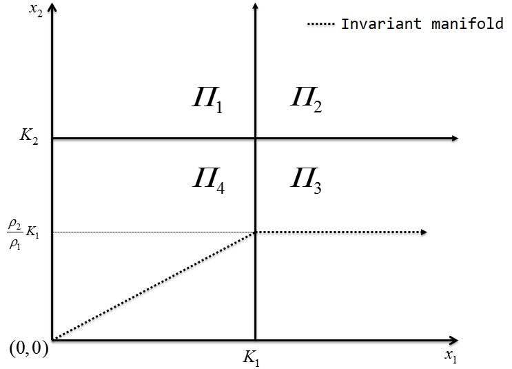
Figure 2: The regions $\varPi_{i}$ and the invariant manifold.

Let $y(0)=(y_{1}(0),y_{2}(0))^{T}\in\mathbb{R}_{+}^{2}.$ We solve the time-changed ODE, which is given by (3.14), in regions $\varPi_{3}$ and $\varPi_{4}$ (considering these two regions only is sufficient for our purposes). It is useful to observe the relations between the coefficients of matrix $\Xi$ in (3.14), which we use later. We know by the definition of the total arrival rate that

$$\rho_{2}(1-p_{22})=\frac{\lambda_{2}}{\mu_{2}}+\frac{p_{12}\gamma_{1}}{\mu_{2}}.$$ (3.16)

The constant $\xi_{22}$ can be expressed as

$$\begin{split}\xi_{22}=\lambda_{2}+\mu_{2}(p_{22}-1)\overset{\eqref{eq:arrival rate 2}}{=}\lambda_{2}-\frac{1}{\rho_{2}}(\lambda_{2}+p_{12}\gamma_{1})=-\frac{\rho_{1}}{\rho_{2}}\xi_{21}<0.\end{split}$$ (3.17)

In a similar way, we can obtain

$$\xi_{11}=-\frac{\rho_{2}}{\rho_{1}}\xi_{12}<0.$$ (3.18)

By definition (2.12), $\tau_{2}$ can be written as $\tau_{2}(1-p_{22})=\beta_{2}+p_{21}\tau_{1}.$ Also, by (2.2) and (2.12), we have that $\tau^{T}\lambda=\beta^{T}(I-P^{T})^{-1}\lambda=\beta^{T}\gamma=1.$ Combining the previous two equations, we get

$$\xi_{12}=-\frac{\tau_{2}}{\tau_{1}}\xi_{22}.$$

Last, by (3.17) and (3.18) we have that

$$\xi_{21}=-\frac{\tau_{1}}{\tau_{2}}\xi_{11}.$$

3.3.1 Solution in region $\varPi_{3}$

Assuming that $y(s)$ is in region $\varPi_{3}$ for $s\in[0,t]$, we can directly solve the second equation of system (3.14) since it is independent of $y_{1}(t)$:

$$y_{2}^{\prime}(t)=\xi_{21}K_{1}+\xi_{22}y_{2}(t).$$

Then, by using (3.17), the solution is given by

$$y_{2}(t)=(y_{2}(0)-\frac{\rho_{2}}{\rho_{1}}K_{1})\exp\{\xi_{22}t\}+\frac{\rho_{2}}{\rho_{1}}K_{1}.$$

Now, we can easily obtain the solution of the first equation of system (3.14). By the relations between the coefficients of (3.14), this solution is given by

$$y_{1}(t)=-\frac{\tau_{2}}{\tau_{1}}(y_{2}(0)-\frac{\rho_{2}}{\rho_{1}}K_{1})\exp\{\xi_{22}t\}+\frac{\bar{W}_{Tot}(0)-w^{*}}{\tau_{1}}+K_{1}.$$ (3.19)

3.3.2 Solution in region $\varPi_{4}$

Assuming that $y(s)$ is in region $\varPi_{4}$ for $s\in[0,t]$, the system given by (3.14) can be written as

$$y^{\prime}(t)=\Xi y(t)^{T}.$$ (3.20)

The eigenvalues of $\Xi$ are $\alpha_{1}=0$ and $\alpha_{2}=\xi_{11}+\xi_{22}=\lambda_{1}+\mu_{1}(p_{11}-1)+\lambda_{2}+\mu_{2}(p_{22}-1)<0.$ Let $V_{1}$, $V_{2}$ be the corresponding eigenvectors; i.e., $V_{1}=\begin{pmatrix}1\\ -\frac{\xi_{11}}{\xi_{12}}\end{pmatrix}$ and $V_{2}=\begin{pmatrix}1\\ \frac{\alpha_{2}-\xi_{11}}{\xi_{12}}\end{pmatrix}=\begin{pmatrix}1\\ \frac{\xi_{21}}{\xi_{11}}\end{pmatrix}.$
Using the relations between the coefficients of matrix $\Xi$, the solution of (3.20) is given by

$$y_{1}(t)= c_{2}+c_{2}^{\prime}\exp\{\alpha_{2}t\},$$ (3.21)

$$y_{2}(t)= c_{2}\frac{\rho_{2}}{\rho_{1}}-c_{4}^{\prime}\frac{\tau_{1}}{\tau_{2}}\exp\{\alpha_{2}t\},$$

with $c_{2}=\frac{\bar{W}_{Tot}(0)}{w^{*}}K_{1}$ and $c_{2}^{\prime}=-\Big{[}y_{2}(0)-\frac{\rho_{2}}{\rho_{1}}y_{1}(0)\Big{]}\Big{[}\frac{\tau_{2}\rho_{1}}{\tau_{1}\rho_{1}+\tau_{2}\rho_{2}}\Big{]}.$

Having found the solution of (3.14) in each region $\varPi_{3}$ and $\varPi_{4}$, we observe that the 2-dimensional equation can be reduced to a 1-dimensional equation since $\bar{W}_{Tot}(0)=\tau_{1}y_{1}(t)+\tau_{2}y_{2}(t),$ for $t\geq 0.$ Now, it is enough to show the convergence of this equation. To see this, define $x(\cdot)$ as

$$x(t)\mathrel{\mathop{\mathchar 58\relax}}=y_{2}(t)=\frac{\bar{W}_{Tot}(0)}{\tau_{2}}-\frac{\tau_{1}y_{1}(t)}{\tau_{2}},$$ (3.22)

and its derivative as

$$x^{\prime}(t)=-\frac{\tau_{1}y^{\prime}_{1}(t)}{\tau_{2}}.$$ (3.23)

Using the observation that we can reduce the dimension by one and the solutions to system (3.14), we show that the fluid model solutions converge to an equilibrium state uniformly for all initial states within a compact set. First, we find the sign of the derivative of the above reduced equation. Then, as the limiting point depends on the sign of the quantity $\bar{W}_{Tot}(0)-w^{*},$ we have to distinguish between the following three cases: the total workload in the fluid model is i) greater than, ii) less than or iii) equal to the critical workload.

3.4 Local analysis: establishing monotonicity

By (3.22), it is clear that we need to study only the behaviour of $y_{1}(t).$ In the sequel, we find the sign of (3.23) in each region $\varPi_{i},$ for $i=1,\ldots,4$.

In region $\varPi_{1}$, we know that $y_{1}(t)\leq K_{1}$. By (3.14) and (3.18), we have that

$$\begin{split}x^{\prime}(t)&=-\frac{\tau_{1}y^{\prime}_{1}(t)}{\tau_{2}}=-\frac{\tau_{1}}{\tau_{2}}(\xi_{11}y_{1}(t)+\xi_{12}K_{2})=-\frac{\tau_{1}}{\tau_{2}}\xi_{12}(-\frac{\rho_{2}}{\rho_{1}}y_{1}(t)+K_{2})\\ &\leq-\frac{\tau_{1}}{\tau_{2}}\xi_{12}(-\frac{\rho_{2}}{\rho_{1}}K_{1}+K_{2})=-\epsilon_{1}<0,\end{split}$$

where $\epsilon_{1}=\frac{\tau_{1}}{\tau_{2}}\xi_{12}(-\frac{\rho_{1}}{\rho_{2}}K_{1}+K_{2}),$ which is strictly positive by (2.4) and the fact that $\xi_{12}>0$. Therefor we conclude that the derivative of $x(t)$ is strictly negative in region $\varPi_{1}.$

In region $\varPi_{2},$ by (3.14) and (3.18), we have that

$$\begin{split}x^{\prime}(t)=-\frac{\tau_{1}}{\tau_{2}}(\xi_{11}K_{1}+\xi_{12}K_{2})=-\frac{\tau_{1}\xi_{12}}{\tau_{2}}(-\frac{\rho_{2}}{\rho_{1}}K_{1}+K_{2})=-\epsilon_{1}<0.\end{split}$$

Thus, the derivative of $x(t)$ is strictly negative for all $y_{1}(0)$ in regions $\varPi_{1}$ and $\varPi_{2}.$ In other words, the trajectory of $x(t)$ leaves regions $\varPi_{1}$ and $\varPi_{2}$ after a finite time. Now, we move to the regions where the invariant points lie, i.e., $\varPi_{3}$ and $\varPi_{4}$.

In region $\varPi_{3}$, by (3.11) and (3.19), we obtain

$$\begin{split}x^{\prime}(t)=\frac{\tau_{1}}{\tau_{2}}\xi_{22}(\frac{\bar{W}_{Tot}(0)}{\tau_{1}}-y_{1}(0)-\frac{\tau_{2}}{\tau_{1}}\frac{\rho_{2}}{\rho_{1}}K_{1})\exp\{\xi_{22}t\}=\frac{\tau_{1}}{\tau_{2}}\xi_{22}(\frac{\bar{W}_{Tot}(0)-w*}{\tau_{1}}+K_{1}-y_{1}(0))\exp\{\xi_{22}t\}.\end{split}$$

We saw in (3.17) that $\xi_{22}<0$. We therefore have that in $\varPi_{3}$,

$$x^{\prime}(t)=\left\{\begin{array}[]{ll}>0&\mbox{if }y_{1}(0)>\frac{\bar{W}_{Tot}(0)-w*}{\tau_{1}}+K_{1},\\ <0&\mbox{if }y_{1}(0)<\frac{\bar{W}_{Tot}(0)-w*}{\tau_{1}}+K_{1},\end{array}\right.$$ (3.24)

and $x^{\prime}(t)=0$ if $y_{1}(0)=\frac{\bar{W}_{Tot}(0)-w*}{\tau_{1}}+K_{1}.$

In region $\varPi_{4},$ by (3.11) and (3.21), we have that

$$\begin{split}x^{\prime}(t)&=-\frac{\tau_{1}y^{\prime}_{1}(t)}{\tau_{2}}=-\frac{\tau_{1}}{\tau_{2}}c_{4}^{\prime}\alpha_{2}\exp\{\alpha_{2}t\},\end{split}$$

where

$$\begin{split}c_{4}^{\prime}=-\Big{[}\frac{\bar{W}_{Tot}(0)}{\tau_{2}}-\frac{\tau_{1}}{\tau_{2}}y_{1}(0)-\frac{\rho_{2}}{\rho_{1}}y_{1}(0)\Big{]}\Big{[}\frac{\tau_{2}\rho_{1}}{\tau_{1}\rho_{1}+\tau_{2}\rho_{2}}\Big{]}&=-\Big{[}\frac{\bar{W}_{Tot}(0)}{\tau_{2}}-\frac{\tau_{1}\rho_{1}+\tau_{2}\rho_{2}}{\tau_{2}\rho_{1}}y_{1}(0)\Big{]}\Big{[}\frac{\tau_{2}\rho_{1}}{\tau_{1}\rho_{1}+\tau_{2}\rho_{2}}\Big{]}\\ &=-\Big{[}\bar{W}_{Tot}(0)-\frac{w^{*}}{K_{1}}y_{1}(0)\Big{]}\Big{[}\frac{\rho_{1}}{\tau_{1}\rho_{1}+\tau_{2}\rho_{2}}\Big{]}.\end{split}$$

Recall that from Section 3.3.2, we have that $\alpha_{2}<0$ and thus in $\varPi_{4}$,

$$x^{\prime}(t)=\left\{\begin{array}[]{ll}>0&\mbox{if }y_{1}(0)>\frac{\bar{W}_{Tot}(0)}{w*}K_{1},\\ <0&\mbox{if }y_{1}(0)<\frac{\bar{W}_{Tot}(0)}{w*}K_{1},\end{array}\right.$$ (3.25)

and $x^{\prime}(t)=0$ if $y_{1}(0)=\frac{\bar{W}_{Tot}(0)}{w*}K_{1}.$

Combining (3.24) and (3.4), and keeping in mind that $\Delta_{1}(w)=\frac{\min\{w,w^{\ast}\}}{w^{\ast}}K_{1}+\frac{\max\{w-w^{\ast},0\}}{\tau_{1}}$ we have that in $\varPi_{3}\cup\varPi_{4}$,

$$x^{\prime}(t)=\left\{\begin{array}[]{ll}>0&\mbox{if }y_{1}(0)>\Delta_{1}(\bar{W}_{Tot}(0)),\\ <0&\mbox{if }y_{1}(0)<\Delta_{1}(\bar{W}_{Tot}(0)),\end{array}\right.$$

and $x^{\prime}(t)=0$ if $y_{1}(0)=\Delta_{1}(\bar{W}_{Tot}(0)).$

3.5 Global analysis: convergence to Invariant Manifold

We are now ready to connect all pieces. From the previous section, we know that $x(t)=y_{2}(t)$ must be smaller than $K_{2}$ after a finite time, thus exiting regions $\Pi_{1}$ and $\Pi_{2}$. Therefore, we can focus on the remaining two regions. In order to do so, we need to consider whether $y_{1}(t)$ will eventually be larger than, smaller than, or equal to $K_{1}$. This leads to three cases, treated separately in the remainder of this section.

Case 1: $\bar{W}_{Tot}(0)-w^{*}>0$.

In this case the invariant point (limiting point) lies in region $\varPi_{3}.$ If $y_{1}(0)\in\varPi_{3},$ then we know that $y_{1}(0)\geq K_{1}.$ By (3.19), we have that

$$\begin{split}y_{1}(t)=&-\frac{\tau_{2}}{\tau_{1}}(\frac{\bar{W}_{Tot}(0)}{\tau_{2}}-\frac{\tau_{1}y_{1}(0)}{\tau_{2}}-\frac{\rho_{2}}{\rho_{1}}K_{1})\exp\{\xi_{22}t\}+\frac{\bar{W}_{Tot}(0)-w^{*}}{\tau_{1}}+K_{1}\\ \geq&(-\frac{\bar{W}_{Tot}(0)}{\tau_{1}}+K_{1}+\frac{\tau_{2}\rho_{2}}{\tau_{1}\rho_{1}}K_{1})\exp\{\xi_{22}t\}+\frac{\bar{W}_{Tot}(0)-w^{*}}{\tau_{1}}+K_{1}\\ \geq&(-\frac{\bar{W}_{Tot}(0)}{\tau_{1}}+K_{1}+\frac{w*}{\tau_{1}}-K_{1})\exp\{\xi_{22}t\}+\frac{\bar{W}_{Tot}(0)-w^{*}}{\tau_{1}}+K_{1}\\ \geq&\frac{\bar{W}_{Tot}(0)-w*}{\tau_{1}}(1-\exp\{\xi_{22}t\})+K_{1}\geq K_{1}.\end{split}$$

If $y_{1}(0)\in\varPi_{4},$ then $y_{1}(0)\leq K_{1}.$ Also, by the assumption that $\bar{W}_{Tot}(0)-w^{*}>0$ and the definition of the lifting map (3.12), we have that $y_{1}(0)\leq K_{1}<\Delta_{1}\bar{W}_{Tot}(0).$ This implies that $x(0)\geq\frac{\bar{W}_{Tot}(0)}{\tau_{2}}-\frac{\tau_{1}K_{1}}{\tau_{2}}$ and $x(t)$ is strictly decreasing. In the sequel, we show that there exists a time $t^{*}$ such that $y_{1}(t^{*})=K_{1}.$ This means that the function $x(t)$ lies in region $\varPi_{3}$ after that time. It is enough to prove that the equation $y_{1}(t)=K_{1},$ has a positive solution. Note that by (3.21), we have that

$$\begin{split}y_{1}(t)&=\frac{\bar{W}_{Tot}(0)}{w^{*}}K_{1}-\Big{[}\bar{W}_{Tot}(0)-\frac{w^{*}}{K_{1}}y_{1}(0)\Big{]}\Big{[}\frac{\rho_{1}}{\tau_{1}\rho_{1}+\tau_{2}\rho_{2}}\Big{]}\exp\{\alpha_{2}t\}.\end{split}$$

Now, setting $y_{1}(t)=K_{1},$ the previous equation becomes

$$\begin{split}\frac{\bar{W}_{Tot}(0)}{w^{*}}K_{1}-K_{1}&=\Big{[}\bar{W}_{Tot}(0)-\frac{w^{*}}{K_{1}}y_{1}(0)\Big{]}\Big{[}\frac{\rho_{1}}{\tau_{1}\rho_{1}+\tau_{2}\rho_{2}}\Big{]}\exp\{\alpha_{2}t\}.\end{split}$$ (3.26)

We argue that (3.26) is satisfied by a $t\geq 0$ as follows. Observe that by (3.11) the quantity $\frac{\rho_{1}}{\tau_{1}\rho_{1}+\tau_{2}\rho_{2}}$ is equal to $\frac{K_{1}}{w^{*}},$ and by the assumption that $y_{1}(0)\in\varPi_{4}$, we have that $y_{1}(0)\leq K_{1}$. Now, we can obtain the following inequality

$$\Big{[}\bar{W}_{Tot}(0)-\frac{w^{*}}{K_{1}}y_{1}(0)\Big{]}\Big{[}\frac{\rho_{1}}{\tau_{1}\rho_{1}+\tau_{2}\rho_{2}}\Big{]}\geq\Big{[}\frac{\bar{W}_{Tot}(0)}{w^{*}}K_{1}-K_{1}\Big{]},$$

which proves the statement. Note that if the total workload is equal to the critical workload, then (3.26) does not have a positive solution since (3.26) would imply that $\exp\{\alpha_{2}t\}=0$. It would only be satisfied by $t=0$. This means, that if $y_{1}(0)\in\varPi_{4}$ and $\bar{W}_{Tot}(0)-w^{*}=0,$ then the function $x(t)$ remains in region $\varPi_{4}$ for ever. Since in this first case $\bar{W}_{Tot}(0)-w^{*}>0$, we have that $\frac{\bar{W}_{Tot}(0)}{w^{*}}K_{1}-K_{1}>0$. Thus, by combining the fact that $y_{1}(0)\leq K_{1}$ and the previous display, we have shown that $\bar{W}_{Tot}(0)-\frac{w^{*}}{K_{1}}y_{1}(0)>\bar{W}_{Tot}(0)-w^{*}>0.$ Combining these arguments leads to the conclusion that the equation $y_{1}(t^{*})=K_{1}$ has a (unique) positive solution, say $t^{*}$. Therefore, $y(t)\in\varPi_{3}$ for $t>t^{*}$. In other words, it is enough to prove that for $\bar{W}_{Tot}(0)-w^{*}>0$, the function $x(t)$ converges to a point in region $\varPi_{3}$.

We now show that it converges to the invariant manifold in region $\varPi_{3}$. By (3.12), we have that $\Delta_{2}\bar{W}_{Tot}(0)=\frac{\rho_{2}}{\rho_{1}}K_{1}.$ By (3.19) and (3.22),

$$|x(t)-\Delta_{2}\bar{W}_{Tot}(0)|\leq\big{|}(\frac{\bar{W}_{Tot}(0)}{\tau_{2}}-\frac{\tau_{1}y_{1}(0)}{\tau_{2}}-\frac{\rho_{2}}{\rho_{1}}K_{1})\big{|}\exp\{\xi_{22}t\}$$

and recall that $\xi_{22}<0.$ Also, for any closed and bounded interval of the form $[0,M]$ for $M>0$, we have that the quantity $|(\frac{\bar{W}_{Tot}(0)}{\tau_{2}}-\frac{\tau_{1}y_{1}(0)}{\tau_{2}}-\frac{\rho_{2}}{\rho_{1}}K_{1})|$ is uniformly bounded by $\sup_{y_{1}(0)\in[0,M]}|(\frac{\bar{W}_{Tot}(0)}{\tau_{2}}-\frac{\tau_{1}y_{1}(0)}{\tau_{2}}-\frac{\rho_{2}}{\rho_{1}}K_{1})|.$ That is, the convergence is uniform for any initial state in a compact set.

Case 2: $\bar{W}_{Tot}(0)-w^{*}<0.$

Adapting the previous case, we first show that if $\bar{W}_{Tot}(0)-w^{*}<0$ and $y_{1}(0)\in\varPi_{4},$ the the function $x(t)$ remains for ever in region $\varPi_{4}.$ To see this, by (3.21) we have that

$$\begin{split}y_{1}(t)&=\frac{\bar{W}_{Tot}(0)}{w^{*}}K_{1}-\Big{[}\bar{W}_{Tot}(0)-\frac{w^{*}}{K_{1}}y_{1}(0)\Big{]}\frac{K_{1}}{w^{*}}\exp\{\alpha_{2}t\}.\end{split}$$

Observing that $y_{1}(0)\leq K_{1}$ in $\varPi_{4}$, we derive the following inequality

$$\begin{split}y_{1}(t)\leq\frac{\bar{W}_{Tot}(0)}{w^{*}}K_{1}+\Big{[}(1-\frac{\bar{W}_{Tot}(0)}{w^{*}})K_{1}\Big{]}\exp\{\alpha_{2}t\}.\end{split}$$

Note that the term $(1-\frac{\bar{W}_{Tot}(0)}{w^{*}})$ is positive by the assumption $\bar{W}_{Tot}(0)-w^{*}<0$ and that $\exp\{\alpha_{2}t\}\leq 1$. Combining these three facts, we have that $y_{1}(t)\leq K_{1}$.

Now, we show that if the process starts in region $\varPi_{3}$ and $\bar{W}_{Tot}(0)-w^{*}<0,$ then there exists a finite time $t^{**}$ such that $x(t)\in\varPi_{4}$ after that time. Again, here we prove that the equation $y_{1}(t^{*})=K_{1}$ has a positive solution. Then, the result follows by observing that $y_{1}(0)\geq K_{1}>\Delta_{1}\bar{W}_{Tot}(0),$ and in that case $x(t)$ is an increasing function. By (3.19), we have that

$$\begin{split}y_{1}(t)&=-\frac{\tau_{2}}{\tau_{1}}(\frac{\bar{W}_{Tot}(0)}{\tau_{2}}-\frac{\tau_{1}y_{1}(0)}{\tau_{2}}-\frac{\rho_{2}}{\rho_{1}}K_{1})\exp\{\xi_{22}t\}+\frac{\bar{W}_{Tot}(0)-w^{*}}{\tau_{1}}+K_{1}\\ &=-\big{(}\frac{\bar{W}_{Tot}(0)-w^{*}}{\tau_{1}}+K_{1}-y_{1}(0)\big{)}\exp\{\xi_{22}t\}+\frac{\bar{W}_{Tot}(0)-w^{*}}{\tau_{1}}+K_{1}.\end{split}$$

Setting $y_{1}(t)=K_{1},$ we obtain

$$\begin{split}\frac{\bar{W}_{Tot}(0)-w^{*}}{\tau_{1}}&=\big{(}\frac{\bar{W}_{Tot}(0)-w^{*}}{\tau_{1}}+K_{1}-y_{1}(0)\big{)}\exp\{\xi_{22}t\}.\end{split}$$ (3.27)

To show that the previous equation has a positive solution, it is enough to show that

$$\begin{split}\frac{\tau_{1}}{\bar{W}_{Tot}(0)-w^{*}}\big{(}\frac{\bar{W}_{Tot}(0)-w^{*}}{\tau_{1}}+K_{1}-y_{1}(0)\big{)}\geq 1.\end{split}$$

Recall that $y_{1}(0)\geq K_{1}$ and that$\bar{W}_{Tot}(0)-w^{*}<0$. We can now derive the previous inequality by observing that

$$\begin{split}\frac{\tau_{1}}{\bar{W}_{Tot}(0)-w^{*}}\big{(}\frac{\bar{W}_{Tot}(0)-w^{*}}{\tau_{1}}+K_{1}-K_{1}\big{)}\geq 1.\end{split}$$

Analogously with the previous case, we note that if the total workload is equal to the critical workload, (3.27) does not have a positive solution. This means, that if $y_{1}(0)\in\varPi_{3}$ and $\bar{W}_{Tot}(0)-w^{*}=0,$ then the function $x(t)$ remains in region $\varPi_{3}$ for ever.

For the convergence to the invariant manifold, we have that $\Delta_{2}\bar{W}_{Tot}(0)=\frac{\rho_{2}}{\rho_{1}}\frac{\bar{W}_{Tot}(0)}{w^{*}}K_{1}$ by (3.12). Moreover, (3.21) and (3.22) lead to

$$|x(t)-\Delta_{2}\bar{W}_{Tot}(0)|\leq\big{|}\frac{\tau_{1}}{\tau_{2}}(\frac{\bar{W}_{Tot}(0)w^{*}}{w^{*}K_{1}}-y_{1}(0))\big{|}\exp\{\alpha_{2}t\}$$

and recall that $\alpha_{2}<0$. The uniform convergence in a compact set for any initial state follows for the same reason as in previous case.

Case 3: $\bar{W}_{Tot}(0)-w^{*}=0.$

In this case, the convergence follows from the comments we made in the previous two cases. If $\bar{W}_{Tot}(0)-w^{*}=0,$ then the function $x(\cdot)$ always stays in the region where $y_{1}(0)$ lies (see comments after (3.26) and (3.27)). As we see, the function converges in regions $\varPi_{3}$ and $\varPi_{4}.$

This concludes the proof of Theorem 3.4, which will be applied to prove a diffusion theorem for the queue length process in the next section.

4 Diffusion approximations

The main objective in this section is to show a state-space collapse property (SSC) for the diffusion queue length process. This yields a diffusion limit theorem for the diffusion-scaled process. To do it, we follow the strategy set up in [1]. Let us consider a family of single-server systems indexed by $n\in\mathbb{N},$ where $n$ tends to infinity, with the same basic structure as that of the network described in Section 2. To indicate the position in the sequence of networks, a superscript $n$ will be appended to the network parameters and processes. Diffusion (or central limit theorem) scaling is indicated by placing a hat over a process. Thus, the well-known diffusion scaling is given by $\widehat{\mathfrak{X}}^{n}(\cdot)=\frac{1}{n}\mathfrak{X}^{n}(n^{2}\cdot).$ Let $\rho^{n}=\sum_{i=1}^{2}\rho_{i}^{n}=(\gamma^{n})^{T}\beta$. We set $\gamma^{n}=(I-P^{T})^{-1}\lambda^{n}$, $\lambda^{n}=\lambda(1-\frac{\theta}{n})$, $\mu^{n}\equiv\mu$, $P^{n}\equiv P$, and $K_{i}^{n}=nK_{i},$ where $\theta$ is a positive real number. Thus, we have that $\rho^{n}=1-\frac{\theta}{n}.$ It is clear that under the critical loading assumption, $\lambda^{n}\rightarrow\lambda$ and $n(1-\rho^{n})\rightarrow\theta,$ as $n\rightarrow\infty$. These are our heavy traffic assumptions. Furthermore, we assume that $\bar{Q}^{n}(0)=\frac{1}{n}Q^{n}(0)\rightarrow\bar{Q}(0),$ where $\bar{Q}(0)$ is a positive constant. The service allocation function for the $n^{\text{th}}$ model is given by

$$R^{n}_{i}(q)=\left\{\begin{array}[]{ll}\frac{\min_{i}\{{q_{i}},{nK_{i}}\}}{\sum_{j=1}^{I}\min\{{q_{j}},{nK_{j}}\}}&\mbox{if }q_{i}\neq 0,\\ 0&\mbox{if }q_{i}=0,\end{array}\right.$$

where we observe that $R^{1}_{i}(\cdot)=R_{i}(\cdot)$. Recall that $R(\cdot)$ is a Lipschitz-continuous function on $\mathbb{R}^{2}_{+}\backslash\{0\}$ and observe that the following scaling property holds: $R^{n}(n\cdot)=R(\cdot)$. In the sequel, we state the technical assumptions that allow us to apply the functional central limit theorem and Bramson’s weak law estimates. We assume that for $i=1,2$,

$$\frac{u_{i}^{n}(1)}{n}\rightarrow 0\quad\text{and}\quad\frac{v^{(1),n}_{ii}(1)}{n}\rightarrow 0,$$

in probability as $n\rightarrow\infty$. In addition, we assume that there exists a function $\eta(\cdot),$ with zero limit at infinity such that for $j>1,$ $i,l\in\{1,2\}$ and $k\in\mathbb{N},$

$$\mathbb{E}(u_{i}^{n}(j)^{2}\mathds{1}_{\{u_{i}^{n}(j)>a\}})\leq\eta(a)\quad\text{and}\quad\mathbb{E}(v^{(k),n}_{il}(j)^{2}\mathds{1}_{\{v^{(k),n}_{il}(j)>a\}})\leq\eta(a).$$

More details about these assumption can be found in [1] and [17]. In the rest of this section, we assume that the previous assumptions are satisfied without refer to them again. The main result in this section is the following

Theorem 4.1.

Assume that the diffusion-scaled initial state converges in distribution as $n\to\infty$, i.e. $\widehat{Q}^{n}(0)\overset{d}{\rightarrow}\Delta\widehat{W}_{Tot}(0),$ where “$\overset{d}{\rightarrow}$” denotes convergence in distribution. Then, the diffusion-scaled stochastic process converges in distribution as $n\to\infty$, i.e.

$$\widehat{Q}^{n}(\cdot)\overset{d}{\rightarrow}\Delta\widehat{W}_{Tot}(\cdot),$$

where $\widehat{W}_{Tot}(t)$ is a 1-dimensional Brownian motion with drift $-\theta$ and variance $\sigma^{2}=\sum_{i=1}^{2}\lambda_{i}\sigma_{s_{i}}^{2}+\tau_{i}^{2}\lambda_{i}c_{u_{i}}^{2},$ where $\sigma_{s_{i}}^{2}$ denotes the variance of $s_{i}(j)$ and $c_{u_{i}}$ denotes the coefficient of variation of $u_{i}(j).$

The proof of this theorem is given in the end of this section. This theorem can be applied to develop heavy traffic approximations for the joint queue length process, as they are both a piece-wise linear function of a one-dimensional RBM, of which the time-dependent distribution can be expressed in closed form (in terms of the Gaussian cdf and pdf); cf. [2]. To see this, note that the functions $\Delta_{1}$ and $\Delta_{2}$ are invertible with inverses

$$\begin{split}\Delta_{1}^{-1}(w)&=\left\{\begin{array}[]{ll}\frac{ww^{*}}{K_{1}}&\mbox{if }w<w^{*},\\ \tau_{1}(w-K_{1})+w^{*}&\mbox{if }w\geq w^{*},\end{array}\right.\\ \Delta_{2}^{-1}(w)&=\left\{\begin{array}[]{ll}\frac{\rho_{1}ww^{*}}{\rho_{2}K_{1}}&\mbox{if }w<w^{*},\\ \infty&\mbox{if }w\geq w^{*}.\end{array}\right.\end{split}$$

We know that $\widehat{W}_{Tot}(t)$ is a RBM$(-\theta,\sigma^{2}).$ Let $\widehat{Q}(\cdot)$ be the diffusion limit. We have that for $x,y\geq 0,$

$$\begin{split}\mathbb{P}{(\widehat{Q}_{1}(t)>x,\widehat{Q}_{2}(t)>y)}=\mathbb{P}{(\Delta_{1}\widehat{W}_{Tot}(t)>x,\Delta_{2}\widehat{W}_{Tot}(t)>y)}=&\mathbb{P}{(\widehat{W}_{Tot}(t)>\Delta_{1}^{-1}(x),\widehat{W}_{Tot}>\Delta_{2}^{-1}(y))}\\ =&\mathbb{P}{(\widehat{W}_{Tot}(t)>z)},\end{split}$$

where $z=\max\{\Delta_{1}^{-1}(x),\Delta_{2}^{-1}(y)\}.$ The last expression can be written in terms of the Gaussian cdf and pdf; cf. [2]. Also, using a similar coupling argument as in [20], it can be shown that one can interchange the steady-state and heavy traffic limits in this case. For space considerations we will leave this as detail to the reader.

The rest of this section is devoted to a proof of Theorem 4.1. It is organized as follows.

1. We first prove a heavy traffic limit theorem for the total workload process.

2. After that, we define a family of shifted fluid-scaled processes in Section 4.2 and we show that they are stochastically bounded in Section 4.3.

3. In Section 4.4, we establish some technical auxiliary estimates and tightness of these families. Moreover, we establish that limit points of these fluid scaled processes, which are called fluid limits, are in fact fluid model solutions as defined in Section 3. The development in this section is very similar to those in Bramson [1] and is therefore kept concise.

4. In Section 4.5, we establish a similar tightness property for a family of shifted fluid-scaled workload processes.

5. The proof is then completed by showing a state-space collapse result in Section 4.6.

4.1 Convergence of the total workload

Lemma 4.2.

Under the critical loading assumption, the diffusion-scaled total workload, $\widehat{W}^{n}_{Tot}(t)=\frac{1}{n}\widehat{W}^{n}_{Tot}(n^{2}t)$, converges in distribution to a RBM$(-\theta,\sigma^{2})$.

Proof.

By (2.11) for $i,l=1,2$ and $i\neq l,$ we have that the total service requirement of the $j^{\text{th}}$ external customer (including customers who already are in queue $i$ at time zero) who enter at queue $i$ is given by

$$s_{i}(j)=v_{ii}^{(1)}(j)+\sum_{k=1}^{\infty}\varphi^{(k)}_{ii}(j)v_{ii}^{(k+1)}(j)+\varphi^{(k)}_{il}(j)v_{il}^{(k+1)}(j).$$

We define the following process

$$W_{G}(t)\mathrel{\mathop{\mathchar 58\relax}}=\sum_{i=1}^{2}\sum_{j=1}^{Q_{i}(0)+E_{i}(t)}s_{i}(j)-\int_{0}^{t}\mathds{1}_{\{W_{G}(s)>0\}}ds.$$ (4.1)

We recall that $E_{i}(\cdot)$ denotes the external arrivals at queue $i$ and by construction of the model, $\{s_{i}(j)\}_{j=1}^{\infty}$ is a sequence of positive i.i.d. random variables for $i=1,2$. The process given in (4.1) represents the workload of a single queue with input given by two independent renewal process that have independent service requirements from each other. The busy time of this system is $\int_{0}^{t}\mathds{1}_{\{W_{G}(s)>0\}}ds=T_{1}(t)+T_{2}(t)$, and it represents the busy time of server in layer 2. Note that the busy time is zero if and only if both queues are empty. The diffusion-scaled process (after subtracting and adding the means of the random quantities in (4.1)), is given by

$$\begin{split}\widehat{W}^{n}_{G}(t)&=\sum_{i=1}^{2}\frac{1}{n}\Big{(}\sum_{j=1}^{n^{2}(\bar{Q}^{n}_{i}(0)+\bar{E}^{n}_{i}(t))}s^{n}_{i}(j)-\tau_{i}n^{2}(\bar{Q}^{n}_{i}(0)+\bar{E}^{n}_{i}(t))\Big{)}\\ &{\hskip 5.0pt}+\tau_{i}(\widehat{E}^{n}_{i}(t)-\lambda^{n}_{i}nt)+\tau_{i}\bar{Q}^{n}_{i}(0)+\tau_{i}\lambda^{n}_{i}nt-nt+\widehat{Y}^{n}(t),\end{split}$$

where $\widehat{Y}^{n}(t)=\int_{0}^{t}\mathds{1}_{\{\widehat{W}^{n}_{G}(s)=0\}}ds$. By the time change theorem in [13] and the functional central limit theorem (also see [2, Theorem 6.8]), we have that $\widehat{W}^{n}_{G}(\cdot)\overset{d}{\rightarrow}\widehat{W}_{G}(\cdot),$ as $n\rightarrow\infty$. Furthermore, the limit can be described as

$$\begin{split}\widehat{W}_{G}(t)=\sum_{i=1}^{2}\tau_{i}\bar{Q}_{i}(0)-\theta t+\sqrt{\lambda_{1}\sigma_{s_{1}}^{2}}\mathcal{W}_{1}(t)+\sqrt{\lambda_{2}\sigma_{s_{2}}^{2}}\mathcal{W}_{2}(t)+\tau_{1}\sqrt{\lambda_{1}c_{u_{1}}^{2}}\mathcal{W}_{3}(t)+\tau_{2}\sqrt{\lambda_{2}c_{u_{2}}^{2}}\mathcal{W}_{4}(t)+\widehat{Y}(t),\end{split}$$

where $\mathcal{W}_{i}(t),$ $1\leq i\leq 4$ are independent 1-dimensional standard Brownian motions and $\widehat{Y}(t)$ can be increased only if $\widehat{W}_{G}(t)=0.$ Thus, the process $\widehat{W}_{G}(t)$ satisfies a 1-dimensional Skorokhod problem. That is, $\widehat{W}_{G}(t)$ is a reflected Brownian motion starting at point $\sum_{i=1}^{2}\tau_{i}\bar{Q}_{i}(0)$ with drift $-\theta$ and variance $\sigma^{2}$ which is given by $\sigma^{2}=\sum_{i=1}^{2}\lambda_{i}\sigma_{s_{i}}^{2}+\tau_{i}^{2}\lambda_{i}c_{u_{i}}^{2},$ where $\sigma_{s_{i}}^{2}$ denotes the variance of $s_{i}(j)$ and $c_{u_{i}}$ denotes the coefficient of variation of $u_{i}(j)$. The second moment of the random variables $s_{i}(j)$ is given by (2.13). In case of Poisson external arrivals, this result is reduced to the well-known heavy-traffic limit (see e.g. [7, Theorem 2.3]).

Now, we shall prove that

$$W_{Tot}(t)=W_{G}(t),{\hskip 10.0pt}t\geq 0.$$ (4.2)

We do it by showing that we can change the label of how we count the service requirements of the customers in the system. Counting the total service requirements of the external arrivals until time $t$ is the same as counting the immediate and remaining service requirements of the total arrivals in the system until time $t$. Recall that $s_{i}(j)=v_{ii}^{(1)}(j)+s^{\prime}_{i}(j)$ for $i=1,2$, where $s^{\prime}_{i}(j)$ are the future service requirements. If $t=0,$ then we have nothing to prove as $E_{i}(0)=A_{i}(0)=0$. If $t>0$ and $\Phi_{li}\Big{(}S_{l}\big{(}T_{l}(t)\big{)}\Big{)}=0$ for $l,i\in\{1,2\},$ then (4.2) holds as all the departures until time $t$ leave the system and so $s^{\prime}_{i}(j)=0$ for $j=1,\ldots,S_{i}\big{(}T_{i}(t)\big{)}$ and $E_{i}(t)=A_{i}(t)$.

For the general case, we first assume that all customers are routed only one time until the time $t.$ The right-hand side in (4.1) can be written as

$$\begin{split}\sum_{i=1}^{2}\sum_{j=1}^{Q_{i}(0)+E_{i}(t)}v_{ii}^{(1)}(j)+\sum_{j=S_{i}\big{(}\mu_{i}T_{i}(t)\big{)}+1}^{Q_{i}(0)+E_{i}(t)}s^{\prime}_{i}(j)+\sum_{j=1}^{S_{i}\big{(}T_{i}(t)\big{)}}s^{\prime}_{i}(j).\end{split}$$ (4.3)

In order to separate the customers who depart form node $i$ (if they are routed or leave the system), we define the following sets for $i,l\in\{1,2\}$ and $i\neq l,$ $\mathcal{A}^{i}=\{j\mathrel{\mathop{\mathchar 58\relax}}1\leq j\leq S_{i}\big{(}T_{i}(t)\big{)}\},$ which includes all the customers who depart from node $i.$ Customers can be routed at the same node and we denote this set by $\mathcal{A}^{i}_{1}=\{j\in\mathcal{A}^{i}\mathrel{\mathop{\mathchar 58\relax}}\varphi_{ii}(j)=1\}$ or to the other node and we denote this set by $\mathcal{A}^{i}_{2}=\{j\in\mathcal{A}^{i}\mathrel{\mathop{\mathchar 58\relax}}\varphi_{il}(j)=1\}.$ Last, we define the following set $\mathcal{A}^{i}_{3}=\mathcal{A}^{i}\setminus(\mathcal{A}^{i}_{1}\cup\mathcal{A}^{i}_{2}),$ which represents all customers who leave the system. If $j\in\mathcal{A}^{i}_{1},$ then there exist natural numbers $k_{j}^{i}$ such that $S_{i}\big{(}T_{i}(t)\big{)}\leq k_{j}^{i}\leq A_{i}(t)-1$ and

$$s^{\prime}_{i}(j)=v_{ii}^{(1)}(k_{j}^{i}+1)+s^{\prime}_{i}(k_{j}^{i}+1).$$

Similarly, if $j\in\mathcal{A}^{i}_{2}$, then for $i\neq l$ there exist $h_{j}^{i},$ such that $S_{l}\big{(}T_{l}(t)\big{)}\leq h_{j}^{i}\leq A_{l}(t)-1$ and

$$s^{\prime}_{i}(j)=v_{ll}^{(1)}(h_{j}^{i}+1)+s^{\prime}_{l}(h_{j}^{i}+1).$$

Last, $j\in\mathcal{A}^{i}_{3}$ means that the $j^{\text{th}}$ customer leaves the system after his first service and so $s^{\prime}_{i}(j)=0$. The quantities $k_{j}^{i}$ and $h_{j}^{i}$ denote the number of customers in node $i=1,2$ (including that one in service) who the $j^{\textrm{th}}$ customer meets after his departure from node $l=1,2$. Therefore, (4.3) can be written as

$$\begin{split}\sum_{i=1}^{2}\sum_{j=1}^{Q_{i}(0)+A_{i}(t)}v_{ii}^{(1)}(j)+\sum_{j=S_{i}\big{(}T_{i}(t)\big{)}+1}^{Q_{i}(0)+A_{i}(t)}s^{\prime}_{i}(j).\end{split}$$

Now, let $k_{0}^{i}(j)$ be the number of routes at node $i,$ for $1\leq j\leq Q_{i}(0)+E_{i}(t)$ until time $t.$ Also, we define the number $k_{0}^{i}=\max_{j}k_{0}^{i}(j),$ and the number of maximum routes for any external arrival in the system until time $t,$ $k_{0}=\max_{i=1,2}\{k_{0}^{i}\}.$ Observe that for any $t\geq 0,$ $k_{0}\in\mathbb{N}$ and it is finite because we assume Markov routing. Take the following partition $[0,t]=\bigcup_{m=0}^{k_{0}}[t_{m},t_{m+1}],$ where $t_{0}=0$ and $t_{{k_{0}+1}}=t$. We take the previous partition in such way, so that in each interval $[t_{m},t_{m+1}],$ any customer in the system can be routed only one time and so that in the interval $[t_{k_{0}},t]$ there is no routing. Now, we can write the right-hand side of (4.1) as

$$\begin{split}\sum_{i=1}^{2}\sum_{j=1}^{Q_{i}(0)+E_{i}(t)}v_{ii}^{(1)}(j)+\sum_{j=S_{i}\big{(}T_{i}(t_{1})\big{)}+1}^{Q_{i}(0)+E_{i}(t)}s^{\prime}_{i}(j)+\sum_{j=1}^{S_{i}\big{(}T_{i}(t_{1})\big{)}}s^{\prime}_{i}(j).\end{split}$$

Applying the previous idea where customers are routed only one time per interval, we have that the above quantity can be written as

$$\begin{split}\sum_{i=1}^{2}\sum_{j=1}^{Q_{i}(0)+E_{i}(t)+\sum_{l=1}^{2}\Phi_{li}\big{(}S_{l}(T_{l}(t_{1}))\big{)}}v_{ii}^{(1)}(j)+\sum_{j=S_{i}\big{(}T_{i}(t_{1})\big{)}+1}^{Q_{i}(0)+E_{i}(t)+\sum_{l=1}^{2}\Phi_{li}\big{(}S_{l}(T_{l}(t_{1}))\big{)}}s^{\prime}_{i}(j)\end{split}$$

Split again the last term of the previous quantity until time $t_{2},$ and apply the previous idea when customers are routed only one time to obtain

$$\begin{split}\sum_{i=1}^{2}\sum_{j=1}^{Q_{i}(0)+E_{i}(t)+\sum_{l=1}^{2}\Phi_{li}\big{(}S_{l}(T_{l}(t_{2}))\big{)}}v_{ii}^{(1)}(j)+\sum_{j=S_{i}\big{(}T_{i}(t_{2})\big{)}+1}^{Q_{i}(0)+E_{i}(t)+\sum_{l=1}^{2}\Phi_{li}\big{(}S_{l}(T_{l}(t_{2}))\big{)}}s^{\prime}_{i}(j).\end{split}$$

Adapting the previous steps until time $t_{k_{0}},$ and recalling that the total arrival process is given by (2.7), we derive (4.2). ∎

In the sequel, this result plays a key role. The next step is to define the so-called shifted fluid-scaled processes and to show that they are stochastically bounded.

4.2 Shifted fluid-scaled processes

We introduce the shifted fluid scaling, which is an extension of the classical fluid scaling. Let $T>0$ and $m\leq nT$. We define

$$\bar{A}_{i}^{n,m}(t)=\frac{1}{n}\Big{(}A_{i}^{n}(nm+nt)-A_{i}^{n}(nm)\Big{)},$$

and the analogous scaling for the processes $T(\cdot)$, $Y_{L_{2}}(\cdot)$, and $E(\cdot)$. For the departure process, the cumulative service time process, and the routing process we have that

$$\bar{S}_{i}^{n,m}(t)=\frac{1}{n}\Big{(}S_{i}^{n}\big{(}nt+T_{i}^{n}(nm)\big{)}-S_{i}^{n}\big{(}T_{i}^{n}(nm)\big{)}\Big{)},$$

$$\bar{V}^{n,m}_{i}(k)=\frac{1}{n}\Big{(}V_{i}^{n}\big{(}nk+S_{i}^{n}(T_{i}^{n}(nm))\big{)}-T_{i}^{n}(nm)\Big{)},$$

$$\bar{\Phi}_{li}^{n,m}(k)=\frac{1}{n}\Phi^{n}_{li}\Big{(}nk+S_{l}^{n}\big{(}T_{l}^{n}(nm)\big{)}\Big{)}-\frac{1}{n}\Phi^{n}_{li}\Big{(}S_{l}^{n}\big{(}T_{l}^{n}(nm)\big{)}\Big{)}.$$

Last, the queue length process is scaled as follows $\bar{Q}_{i}^{n,m}(t)=\frac{1}{n}Q_{i}^{n}(nm+nt)$ and analogously for the scaling of the immediate and total workload. The system dynamics (2.5)–(2.10) under the shifted fluid scaling become

$$\bar{Q}^{n,m}_{i}(t)=\bar{Q}^{n,m}_{i}(0)+\bar{E}^{n,m}_{i}(t)+\sum_{l=1}^{2}\bar{\Phi}_{li}^{n,m}\Big{(}\bar{S}^{n,m}_{l}\Big{(}\bar{T}^{n,m}_{l}(t)\Big{)}\Big{)}-\bar{S}^{n,m}_{i}\Big{(}\bar{T}^{n,m}_{i}(t)\Big{)},$$ (4.4)

$$\bar{T}^{n,m}_{i}(t)=\int_{0}^{t}R^{n}_{i}(n\bar{Q}^{n,m}(s))ds=\int_{0}^{t}R_{i}(\bar{Q}^{n,m}(s))ds,$$ (4.5)

$$\bar{W}^{n,m}_{i}(t)=\bar{V}^{n,m}_{i}\bigg{(}\bar{Q}^{n,m}_{i}(0)+\bar{E}^{n,m}_{i}(t)+\sum_{l=1}^{2}\bar{\Phi}_{li}^{n,m}\Big{(}\bar{S}^{n,m}_{l}\Big{(}\bar{T}^{n,m}_{l}(t)\Big{)}\Big{)}\bigg{)}-\bar{T}^{n,m}_{i}(t),$$ (4.6)

$$\sum_{i=1}^{2}\bar{T}_{i}^{n,m}(t)+\bar{Y}^{n,m}_{L_{2}}(t)=t,$$ (4.7)

$$\bar{Y}^{n,m}_{L_{2}}(t)\textrm{ increases }\Rightarrow\bar{W}_{1}^{n,m}(t)+\bar{W}_{2}^{n,m}(t)=0,\qquad t\geq 0,\ i=1,2.$$

In the sequel, we shall be referring to shifted fluid scaling, and shifted fluid process as shifted scaling, and shifted process for simplicity. The main step of SSC is to show the shifted process can be approximated by a solution of the fluid model. This is done in Section 4.4. We first need to prove that the shifted workload and shifted queue length are bounded at zero, which we do in the following section. Using these bounds and some properties of the cumulative service time (2.6), we can apply the results in [1, Sections 4 and 5].

4.3 Bounding the shifted processes

First, we find the relation between the diffusion scaling and the shifted scaling. Although this relation is easily obtained and is already known in the literature (e.g. [19]), we provide it here for completeness. Fix $L>1$ and define the shifted fluid processes on $[0,L]$. The interval $[0,n^{2}T]$ can be covered by $[nt]+1$ overlapping intervals as follows. For $t\in[0,n^{2}T],$ there exist $s\in[0,L]$ and $m\in\{0,1,\ldots,[nt]\}$ such that

$$n^{2}t=nm+ns.$$

We can write the relation between the diffusion scaling and the shifted scaling as follows. For $s\leq L,$

$$\bar{Q}^{n,m}(s) =\widehat{Q}^{n}\big{(}\frac{nm+ns}{n^{2}}\big{)},$$ (4.8)

$$\bar{W}^{n,m}_{Tot}(s) =\widehat{W}^{n}_{Tot}\big{(}\frac{nm+ns}{n^{2}}\big{)}.$$ (4.9)

By Lemma 4.2 and (4.9), it follows that for any $\epsilon>0$ there exists a constant $B_{1}>0$ such that

$$\liminf_{n\rightarrow\infty}\mathbb{P}(\max_{m\leq nT}\bar{W}^{n,m}_{Tot}(0)\leq B_{1})\geq 1-\epsilon.$$ (4.10)

We denote the event $\{\omega\in\Omega\mathrel{\mathop{\mathchar 58\relax}}\max_{m\leq nT}\bar{W}^{n,m}_{Tot}(0)\leq B_{1}\}$ by $\mathcal{G}_{1}^{n}(B_{1}).$ Using now (4.10), it can be shown that the shifted queue length process is stochastically bounded at zero.

Lemma 4.3.

Let $T>0.$ For any $\epsilon>0$ there exists a constant $B_{2}>0$ such that

$$\liminf_{n\rightarrow\infty}\mathbb{P}(\max_{m\leq nT}\bar{Q}^{n,m}_{i}(0)\leq B_{2})\geq 1-\epsilon,{\hskip 5.0pt}i=1,2.$$ (4.11)

We denote the event $\{\omega\in\Omega\mathrel{\mathop{\mathchar 58\relax}}\max_{m\leq nT}\bar{Q}^{n,m}_{i}(0)\leq B_{2}\}$ by $\mathcal{G}^{n}_{2}(B_{2})$.

Proof.

We prove the result by deriving a contradiction, so suppose that (4.11) does not hold. Thus, assume there exists at least one $i$ such that $Q_{i}^{n,m}(0)$ is not stochastically bounded. In other words, there exists a $\delta>0$ such that for any $B>0$,

$$\liminf_{n\rightarrow\infty}\mathbb{P}\big{(}\max_{m\leq nT}Q_{i}^{n}(nm)>Bn\big{)}>\delta.$$ (4.12)

Suppose that $m_{n}$ is such that it optimises the quantity $\max_{m\leq nT}Q_{i}^{n}(nm)$. We can choose in (4.10), $\epsilon=\frac{\delta}{3}$ and a (large enough) constant $B_{1}$. Also, we choose a constant $B$ such that $B>2\frac{B_{1}}{\beta_{i}}$. By the definition of the total workload (2.14) and (2.15), we have that

$$\max_{m\leq nT}W^{n}_{Tot}(nm) \geq\sum_{j=1}^{S_{i}^{n}(T^{n}_{i}(nm_{n}))+1}v_{ii}^{(1)}(j)-T^{n}_{i}(nm_{n})+\sum_{j=S_{i}^{n}(T^{n}_{i}(nm_{n}))+2}^{S_{i}^{n}(T^{n}_{i}(nm_{n}))+Q_{i}^{n}(nm_{n})}v_{ii}^{(1)}(j)$$

$$\geq\sum_{j=S_{i}^{n}(T^{n}_{i}(nm_{n}))+2}^{S_{i}^{n}(T^{n}_{i}(nm_{n}))+Q_{i}^{n}(nm_{n})}v_{ii}^{(1)}(j).$$

We know that $v_{ii}^{(1)}(j)$ are i.i.d. with mean $\beta_{i}$. Also, in the previous summation $j>S_{i}^{n}(T^{n}_{i}(nm_{n}))$, which means that $v_{ii}^{(1)}(j)$ are independent of the process $S_{i}^{n}(T^{n}_{i}(nm_{n}))$. Define the the following event

$$\mathcal{G}^{n}=\{\omega\in\Omega\mathrel{\mathop{\mathchar 58\relax}}\big{|}\frac{1}{Bn}\sum_{j=S_{i}^{n}(T^{n}_{i}(nm_{n}))+2}^{S_{i}^{n}(T^{n}_{i}(nm_{n}))+Bn}v_{ii}^{(1)}(j)-\beta_{i}\big{|}<\frac{\beta_{i}}{2}\}.$$ (4.13)

By the weak law of large numbers (which we can apply due to the independence of the $v_{ii}^{(1)}(j)$ and $S_{i}^{n}(T^{n}_{i}(nm_{n}))$), we have that for large $n$, $\mathbb{P}(\mathcal{G}^{n})\geq 1-\frac{\delta}{3}$. In the sequel, we assume that $\omega\in\mathcal{G}^{n}\cap\mathcal{G}_{1}^{n}(B_{1})\cap(\mathcal{G}_{2}^{n}(B))^{c}$, and note that $\mathbb{P}{(\mathcal{G}^{n}\cap\mathcal{G}_{1}^{n}(B_{1})\cap(\mathcal{G}_{2}^{n}(B))^{c})}\geq\frac{\delta}{3}$. Applying (4.12) and dividing by $n$ we derive

$$B_{1}\geq\max_{m\leq nT}\bar{W}^{n,m}_{Tot}(0)\geq\frac{B}{Bn}\sum_{j=S_{i}^{n}(T^{n}_{i}(nm_{n}))+2}^{S_{i}^{n}(T^{n}_{i}(nm_{n}))+Bn}v_{ii}^{(1)}(j).$$

By (4.13) and the last inequality, we obtain for sufficiently large $n$, $B_{1}\geq B(\beta_{i}-\frac{\beta_{i}}{2})>2\frac{B_{1}}{2}$. This yields a contradiction. ∎

Having proved that the shifted processes are bounded, we can show that the shifted processes can be approximated by a solution of the fluid model. This is the topic of next section, in which we use a very similar approach as is Bramson [1, Sections 4 and 5].

4.4 Uniform fluid approximation

By [1, Proposition 5.1], we have that for any $\epsilon>0$,

$$\mathbb{P}(\max_{m<nT}\|\bar{E}^{n,m}(\cdot)-\lambda^{n}\cdot\|_{L}>\epsilon)\leq\epsilon.$$ (4.14)

Also, by [1, Proposition 5.2] it is known that the shifted arrival process is almost Lipschitz continuous, which means that for some $N_{1}>0,$

$$\mathbb{P}(\sup_{t_{1},t_{2}\in[0,L]}{|\bar{{E}}^{n,m}(t_{2})-\bar{{E}}^{n,m}(t_{1})|>N_{1}|t_{2}-t_{1}|}+\epsilon\ for\ some\ m<nT)\leq\epsilon.$$

Furthermore, using the definition of the cumulative service time (2.6), the property $\sum_{i=1}^{2}R_{i}^{n}(q)=1$, and the observation that $Y^{n}_{L_{2}}(\cdot)$ and $T^{n}(\cdot)$ are increasing functions in time, we conclude that the shifted process, $T^{n,m}(\cdot),$ and the shifted idle time are Lipschitz continuous with constant equal to 1.

Proposition 4.4.

Let $\epsilon>0$. Then, for an appropriate large $n$, and for $i=1,2$,

$$\mathbb{P}(\max_{m<nT}\|\bar{S}_{i}^{n,m}(\bar{T}_{i}^{n,m}(\cdot))-\mu_{i}\bar{T}_{i}^{n,m}(\cdot)\|_{L}>\epsilon)<\epsilon,$$ (4.15)

$$\mathbb{P}(\max_{m<nT}\|\sum_{l=1}^{2}\bar{\Phi}_{li}^{n,m}\Big{(}\bar{S}^{n,m}_{l}\big{(}\bar{T}^{n,m}_{l}(\cdot)\big{)}\Big{)}-\sum_{l=1}^{2}\mu_{l}p_{li}\bar{T}_{l}^{n,m}(\cdot)\|_{L}>\epsilon)<\epsilon,$$ (4.16)

$$\begin{split}&\mathbb{P}(\max_{m<nT}\|\bar{V}^{n,m}_{i}\bigg{(}\bar{Q}^{n,m}_{i}(0)+\bar{E}^{n,m}_{i}(\cdot)+\sum_{l=1}^{2}\bar{\Phi}_{li}^{n,m}\Big{(}\bar{S}^{n,m}_{l}\big{(}\bar{T}^{n,m}_{l}(\cdot)\big{)}\Big{)}\bigg{)}\\ &\qquad\qquad\qquad-\beta_{i}(\bar{Q}_{i}^{n,m}(0)+\lambda_{i}^{n}\cdot+\sum_{l=1}^{2}p_{li}\bar{T}_{l}^{n,m}(\cdot))\|_{L}>\epsilon)<\epsilon,\\ \end{split}$$ (4.17)

Proof.

It is shown in [1] that for a renewal process $S(\cdot)$,

$$\mathbb{P}\big{(}\sup_{m\leq nT}\sup_{t\leq L}|\frac{1}{n}(S_{i}^{n}((nm+nt))-S_{i}^{n}(nm))-\mu t|_{L}\geq\epsilon)<\epsilon,$$

which is equivalent to (the process can start anywhere in the interval $[0,n^{2}T]$)

$$\mathbb{P}\big{(}\sup_{u\in[0,n^{2}T]}\sup_{t\leq L}|\frac{1}{n}(S_{i}^{n}((u+nt))-S_{i}^{n}(u))-\mu_{i}t|\geq\epsilon)<\epsilon.$$ (4.18)

Let $t^{\prime}=\bar{T}_{i}^{n,m}(t)=\frac{1}{n}(T_{i}^{n}(nm+nt)-T_{i}^{n}(nm))\in[0,L]$ and $u=T_{i}^{n}(nm)\leq n^{2}T$, for $m\leq nT$. By (4.18) we obtain

$$\mathbb{P}\big{(}\sup_{u\in[0,n^{2}T]}\sup_{t^{\prime}\leq L}|\frac{1}{n}(S_{i}^{n}((u+nt^{\prime}))-S_{i}^{n}(u))-\mu_{i}t^{\prime}|\geq\epsilon\big{)}<\epsilon,$$

for each $i=1,2$. Then, (4.15) follows.

By the Lipschitz continuity of the departure process in Proposition 4.5, which we can prove only using (4.15), we know that $\|S_{i}(T_{i}(\cdot))\|_{L}\leq N_{2}Ln$. Using [1, Proposition 4.2], we derive

$$\mathbb{P}(\max_{m<nT}\|\sum_{l=1}^{2}\bar{\Phi}_{li}^{n,0}\Big{(}\bar{S}^{n,0}_{l}\big{(}\bar{T}^{n,0}_{l}(\cdot)\big{)}\Big{)}-\sum_{l=1}^{2}p_{li}\bar{S}_{l}^{n,0}(\bar{T}^{n,0}(\cdot))\|_{L}>N_{2}L\epsilon)<\frac{\epsilon}{n}.$$

Furthermore, using the conclusion of the proof of [1, Proposition 5.19], we obtain

$$\mathbb{P}(\max_{m<nT}\|\sum_{l=1}^{2}\bar{\Phi}_{li}^{n,m}\Big{(}\bar{S}^{n,m}_{l}\big{(}\bar{T}^{n,m}_{l}(\cdot)\big{)}\Big{)}-\sum_{l=1}^{2}p_{li}\bar{S}_{l}^{n,m}(\bar{T}^{n,m}(\cdot))\|_{L}>N_{2}L\epsilon)<\frac{\epsilon}{n}.$$

Applying (4.15) to the last inequality we obtain (4.16).

To prove (4.17), we know by Lemma 4.3, that for some $B_{2}>0$, $|Q^{n}(0)|\leq B_{2}n.$ Using (4.14), (4.17), and applying [1, Proposition 4.2], the result follows. ∎

In the following proposition, we show that all the shifted processes are almost Lipschitz continuous.

Proposition 4.5.

Let $\bar{{X}}^{n,m}(\cdot)$ be any of the processes $\bar{S}^{n,m}(\cdot),$ $\bar{Q}^{n,m}(\cdot)$ and $\bar{W}^{n,m}(\cdot).$ Then for large $n,$ for $\epsilon>0$ and some $N>0,$ we have that

$$\mathbb{P}(\sup_{t_{1},t_{2}\in[0,L]}{|\bar{{X}}^{n,m}(t_{2})-\bar{{X}}^{n,m}(t_{1})|>N|t_{2}-t_{1}|}+\epsilon\ \textrm{for some}\ m<nT)\leq\epsilon.$$ (4.19)

Proof.

For the departure process and by using (4.15), we have for $i=1,2$ that

$$|\bar{S_{i}}^{n,m}(T_{i}^{n,m}(t_{2}))-\bar{S_{i}}^{n,m}(\bar{T}_{i}^{n,m}(t_{1}))|\leq|\bar{S_{i}}^{n,m} (\bar{T}_{i}^{n,m}(t_{2}))-\mu_{i}\bar{T}_{i}^{n,m}(t_{2})|+|\bar{S_{i}}^{n,m}(\bar{T}_{i}^{n,m}(t_{1}))-\mu_{i}\bar{T}_{i}^{n,m}(t_{1})|$$

$$+|\mu_{i}\bar{T}_{i}^{n,m}(t_{2})-\mu_{i}\bar{T}_{i}^{n,m}(t_{1})|\leq N_{2}|t_{2}-t_{1}|+2\epsilon,$$

where $N_{2}=\max_{i}\mu_{i}$. Using (4.14), (4.17), and the Lipschitz continuity of the cumulative service time (2.6), $T(\cdot),$ it is easy to show that the shifted total arrival process, $\bar{A}^{n,m}(\cdot),$ is almost Lipschitz continuous with $N_{3}=N_{1}+\|P\|N_{2}$, where $N_{1}=\max_{i}\lambda_{i}$.

Combining the almost Lipschitz continuity for the shifted arrival and the shifted departure process, $\bar{A}^{n,m}(\cdot),$ $\bar{S}^{n,m}(T(\cdot)),$ the result for the shifted queue length process, $\bar{Q}^{n,m}(\cdot),$ follows with the constant $N_{4}=N_{3}+N_{2}$. Using the same idea and (4.17), we obtain the same result for the shifted immediate workload process, $\bar{W}^{n,m}(\cdot),$ with $N_{5}=\frac{N_{1}}{\min_{i}{\mu_{i}}}+\|P\|.$ ∎

Remark 4.1.

Adapting the techniques in [1] we can replace $\epsilon$ in the propositions above by $\epsilon(n)$ such that $\epsilon(n)\rightarrow 0.$ Let $\mathcal{G}_{i}^{n}\subseteq\Omega$, $1\leq i\leq 5$, be the “good events” such that the complements of inequalities (4.14), (4.15), (4.16), (4.17) and (4.19) hold if we replace $\epsilon$ by $\epsilon(n)$. Also, let $\mathcal{G}_{1}^{n}(B)$ and $\mathcal{G}_{2}^{n}(B)$ be as in (4.10) and (4.11) with $B=\max\{B_{1},B_{2}\}.$ Denote by $\mathcal{G}_{0}^{n}(B)$ the intersection of the previous events. Because $\omega\in\mathcal{G}_{0}^{n}(B)$, we know that $|\bar{\mathfrak{X}}^{n,m}(t_{2})-\bar{\mathfrak{X}}^{n,m}(t_{1})|\leq N|t_{2}-t_{1}|+\epsilon.$ Also, by Lemmas 4.2, 4.3, and by the definition of the shifted processes (4.4)–(4.7), we have that $|\bar{\mathfrak{X}}^{n,m}(0)|\leq B,$ for some positive constant B. In addition, if we replace the bound in [1, Inequality 4.6], by a general real number, we can again show that the set of Lipschitz functions with this property is compact; see [16, Lemma 6.3].

By Remark 4.1, all the requirements in [1, Section 4.1] hold. Thus, we can find a Lipschitz-continuous function $\widetilde{\mathfrak{X}}(\cdot)$, such that for $\epsilon(n)\to 0,$

$$\|\bar{\mathfrak{X}}^{n,m}(\cdot,\omega)-\widetilde{\mathfrak{X}}(\cdot)\|_{L}\leq\epsilon(n),{\hskip 15.0pt}\forall\ \omega\in\mathcal{G}^{n}_{0}(B),\ \forall\ m\leq nT.$$ (4.20)

Proposition 4.6.

The function $\widetilde{\mathfrak{X}}(\cdot)$ is a solution to the fluid model equations on $[0,L]$.

Proof.

We shall show that $\widetilde{\mathfrak{X}}(\cdot)$ verifies the fluid model’s equations (3.2)–(3.6). To do this, let $\delta>0$. As $\epsilon(n)\rightarrow 0,$ we can find large a $n$ such that $\epsilon(n)<\delta.$ It is known by (4.20) that for large $n,$

$$\|\bar{\mathfrak{X}}^{n,m}(\cdot)-\widetilde{\mathfrak{X}}(\cdot)\|_{L}<\delta.$$

Thus, from the heavy traffic assumption, we conclude that $|\lambda^{n}-\lambda|<\delta.$ Using the above inequalities, (4.14), Proposition 4.4, and the triangle inequality it can be proved in the same way as in [1, Proposition 6.2] that all the functions $\widetilde{\mathfrak{X}}(\cdot),$ except for $\widetilde{T}(\cdot),$ verify the fluid model’s equations. To prove that $\widetilde{T}(\cdot)$ satisfies (3.3), we need to use the following two properties of the service allocation function: i) $R^{n}(nq)=R(q)$ and ii) $R(\cdot)$ is a Lipschitz continuous function on $\mathbb{R}^{2}_{+}\backslash\{0\}$; i.e., there exists a constant $C,$ such that for $q_{1},q_{2}\in\mathbb{R}^{2}_{+}\backslash\{0\}$

$$|R(q_{2})-R(q_{1})|\leq C|q_{2}-q_{1}|.$$

Now, using (4.5), and the above properties of the service allocation function, we can show that $\widetilde{T}(\cdot)$ satisfies (3.3) and is thus a solution to the fluid model:

$$\begin{split}|\widetilde{T}(t)-\int_{0}^{t}R(\widetilde{Q}(s))ds|&=|\widetilde{T}(t)-\bar{T}^{n,m}(t)+\int_{0}^{t}R(\bar{Q}^{n,m}(s))ds-\int_{0}^{t}R(\widetilde{Q}(s))ds|\\ &\leq|\widetilde{T}(t)-\bar{T}^{n,m}(t)|+\int_{0}^{t}|R(\bar{Q}^{n,m}(s))-R(\widetilde{Q}(s))|ds\\ &\leq\delta+\int_{0}^{t}C|\bar{Q}^{n,m}(s)-\widetilde{Q}(s)|\leq\delta+\int_{0}^{t}C\delta\leq\delta+CL\delta.\end{split}$$

∎

4.5 The scaled shifted total workload process

In this section, we see that we can approximate the scaled shifted total workload process by a solution to the fluid model. We begin with a preliminary result.

Proposition 4.7.

For appropriately large $n\in\mathbb{N}$ and $\epsilon>0,$ we have that

$$\begin{split}&\mathbb{P}\Big{(}\max_{m<nT}\Big{\|}\sum_{i=1}^{2}\frac{1}{n}\sum_{j=Z^{n,m}_{i}(\cdot)}^{B^{n,m}_{i}(\cdot)}s^{\prime}_{i}(j)-\sum_{k=1}^{\infty}\beta^{T}(P^{T})^{k}\bar{Q}^{n,m}(\cdot)\Big{\|}_{L}>\epsilon\Big{)}<\epsilon,\end{split}$$ (4.21)

where

$$\begin{split}Z^{n,m}_{i}(\cdot)&=n\bar{S}^{n,m}_{i}\big{(}\bar{T}^{n,m}_{i}(\cdot)\big{)}+S^{n}_{i}\big{(}T^{n}_{i}(nm)\big{)}+1,\\ B^{n,m}_{i}(\cdot)&=Q^{n}_{i}(0)+n\bar{A}^{n,m}_{i}(\cdot)+A^{n}_{i}(nm).\end{split}$$

Proof.

The random variables $s^{\prime}_{i}(j)$ depend on $n$, but to keep the notation simple we omit the index $n$. Note that (4.21) can be written as

$$\begin{split}&\mathbb{P}\Big{(}\max_{m<nT}\Big{\|}\sum_{i=1}^{2}\frac{1}{n}\sum_{j=Z^{n,m}_{i}(\cdot)}^{B^{n,m}_{i}(\cdot)}s^{\prime}_{i}(j)-\sum_{k=1}^{\infty}\beta^{T}\bar{p}_{i}^{(k)}\bar{Q}_{i}^{n,m}(\cdot)\Big{\|}_{L}>\epsilon\Big{)}<\epsilon,\\ \end{split}$$

where $\beta^{T}\bar{p}^{(k)}_{i}=\beta_{1}p^{(k)}_{i1}+\beta_{2}p^{(k)}_{i2}.$ We have that

$$\begin{split}&\mathbb{P}\Big{(}\max_{m<nT}\Big{\|}\sum_{i=1}^{2}\frac{1}{n}\sum_{j=Z^{n,m}_{i}(\cdot)}^{B^{n,m}_{i}(\cdot)}s^{\prime}_{i}(j)-\sum_{k=1}^{\infty}\beta^{T}\bar{p}_{i}^{(k)}\bar{Q}_{i}^{n,m}(\cdot)\Big{\|}_{L}>\epsilon\Big{)}\\ &\quad\leq\sum_{i=1}^{2}\mathbb{P}\Big{(}\max_{m<nT}\Big{\|}\frac{1}{n}\sum_{j=Z^{n,m}_{i}(\cdot)}^{B^{n,m}_{i}(\cdot)}s^{\prime}_{i}(j)-\sum_{k=1}^{\infty}\beta^{T}\bar{p}_{i}^{(k)}\bar{Q}_{i}^{n,m}(\cdot)\Big{\|}_{L}>\frac{\epsilon}{2}\Big{)},\end{split}$$

so it is enough to show that the last term is sufficiently small for $i=1,2$. First, we shall prove it for $m=0.$ We know by Proposition 4.5 that the shifted queue length process is Lipschitz continuous and by Proposition 4.3 that the shifted queue length process at zero is stochastically bounded; i.e., for $t\leq L$, $|Q_{i}^{n}(t)|\leq(N_{4}+B_{2})Ln$. By [1, Proposition 4.2], we derive

$$\begin{split}\mathbb{P}\Big{(}\Big{\|}\sum_{j=S^{n}_{i}\big{(}T^{n}_{i}(\cdot)\big{)}}^{Q^{n}_{i}(0)+A^{n}_{i}(\cdot)}s^{\prime}_{i}(j)-\sum_{k=1}^{\infty}\beta^{T}\bar{p}_{i}^{(k)}Q_{i}^{n}(\cdot)\Big{\|}_{N_{4}Ln}>\frac{\epsilon(N_{4}+B_{2})Ln}{2}\Big{)}\leq\frac{\epsilon}{2(N_{4}+B_{2})Ln},\end{split}$$

which leads to

$$\begin{split}\mathbb{P}\Big{(}\Big{\|}\frac{1}{n}\sum_{j=Z^{n,0}_{i}(\cdot)}^{B^{n,0}_{i}(\cdot)}s^{\prime}_{i}(j)-\sum_{k=1}^{\infty}\beta^{T}\bar{p}_{i}^{(k)}\bar{Q}_{i}^{n,0}(\cdot)\Big{\|}_{L}>\frac{\epsilon(N_{4}+B_{2})L}{2}\Big{)}\leq\frac{\epsilon}{2(N_{4}+B_{2})n},\end{split}$$

where $B^{n,0}_{i}(\cdot)-Z^{n,0}_{i}(\cdot)=\bar{Q}_{i}^{n,0}(\cdot).$ Multipling the error bounds by the number of processes $[nT]+1$ and choosing a suitable $\epsilon$ we derive

$$\begin{split}\mathbb{P}\Big{(}\Big{\|}\frac{1}{n}\sum_{j=Z^{n,0}_{i}(\cdot)}^{B^{n,m}_{i}(\cdot)}s^{\prime}_{i}(j)-\sum_{k=1}^{\infty}\beta^{T}\bar{p}_{i}^{(k)}\bar{Q}_{i}^{n,m}(\cdot)\Big{\|}_{L}>\frac{\epsilon}{2}\Big{)}\leq\frac{\epsilon}{2}.\end{split}$$

∎

Adapting Remark 4.1, we can replace $\epsilon$ in the proposition above $\epsilon$ by $\epsilon(n)$ such that $\epsilon(n)\rightarrow 0$ as $n\rightarrow\infty.$ This will be done in the next result, where we combine all technical estimates so far to construct a “good” event.

Proposition 4.8.

Let $\epsilon>0$ and $\mathcal{G}_{0}^{n}\subseteq\Omega$ be as in Remark 4.1. Let $\mathcal{G}_{6}^{n}\subseteq\Omega$ be the event such that the complement of (4.21) holds if we replace $\epsilon$ by $\epsilon(n)$. Define the event $\mathcal{G}^{n}(B)=\mathcal{G}_{0}^{n}(B)\cap\mathcal{G}_{6}^{n}.$ Then

$$\lim_{n\rightarrow\infty}\mathbb{P}{\big{(}\mathcal{G}^{n}(B)\big{)}}\geq 1-\epsilon.$$

Proof.

Note that $\mathcal{G}^{n}(B)=\bigcap_{i=1}^{6}\mathcal{G}_{i}^{n}\cap\mathcal{G}_{1}^{n}(B)\cap\mathcal{G}_{2}^{n}(B).$ We denote $(\mathcal{G}_{i})^{c}$ the complement of the event $\mathcal{G}_{i}.$ For $1\leq i\leq 6$, we have by construction that $\mathbb{P}{((\mathcal{G}_{i}^{n})^{c})}\leq\epsilon(n).$ Also, by (4.10) and (4.11) we can choose a constant $B$ such that for $i=1,2$

$$\lim_{n\rightarrow\infty}\mathbb{P}{\big{(}\mathcal{G}_{i}^{n}(B)\big{)}}\geq 1-\frac{\epsilon}{2}.$$

Combining the above inequalities, we obtain as $n\rightarrow\infty,$

$$\begin{split}\mathbb{P}{(\mathcal{G}^{n}(B))}=\mathbb{P}{\Big{(}\Big{(}\bigcup_{i=1}^{6}(\mathcal{G}_{i}^{n})^{c}\cup(\mathcal{G}_{1}^{n}(B))^{c}\cup(\mathcal{G}_{2}^{n}(B))^{c}\Big{)}^{c}\Big{)}}=&1-\mathbb{P}{\Big{(}\bigcup_{i=1}^{6}(\mathcal{G}_{i}^{n})^{c}\cup(\mathcal{G}_{1}^{n}(B))^{c}\cup(\mathcal{G}_{2}^{n}(B))^{c}\Big{)}}\\ \geq&1-6\epsilon(n)-\epsilon\rightarrow 1-\epsilon.\end{split}$$

∎

In the sequel, we assume that $\omega\in\mathcal{G}^{n}(B).$ In other words, Proposition 4.8 allows us to use a sample-path approach. As a final step towards proving state-space collapse, we use this approach to show that there exists a fluid approximation for the total workload of the system.

Proposition 4.9.

There exists a solution of the fluid model equations, $\widetilde{W}_{Tot}(\cdot)$, such that for $m\leq nT$

$$\|\bar{W}^{n,m}_{Tot}(\cdot,\omega)-\widetilde{W}_{Tot}(\cdot)\|_{L}\leq\epsilon(n){\hskip 15.0pt}\forall\ \omega\in\mathcal{G}^{n}(B).$$

Proof.

Take $\epsilon>0$ and let $\omega\in\mathcal{G}^{n}(B)$ as defined in Proposition 4.8. Let the functions $\widetilde{Q}(t)$ and $\widetilde{W}(t)$ be such so that they satisfy (4.20). Define the function

$$\widetilde{W}_{Tot}(t)=\beta^{T}(I-P^{T})^{-1}\widetilde{Q}(t),$$

which is a solution to the fluid model equations because $\widetilde{Q}(t)$ is. Omitting again the index $n$ in the quantity $s^{\prime}_{i}(j),$ by the definition of the total workload, we have that

$$\bar{W}^{n,m}_{Tot}(t)=\sum_{i=1}^{2}\bar{W}^{n,m}_{i}(t)+\sum_{i=1}^{2}\frac{1}{n}\sum_{j=Z_{i}^{n,m}(t)}^{B_{i}^{n,m}(t)}s^{\prime}_{i}(j),$$

where the quantities $Z_{i}^{n,m}(t)$ and $B_{i}^{n,m}(t)$ are defined in Proposition 4.7. Using the triangular inequality, we thus have that

$$\begin{split}\Big{\|}\bar{W}_{Tot}^{n,m}(\cdot)-\widetilde{W}_{Tot}(\cdot)\Big{\|}_{L}\leq&\sum_{i=1}^{2}\Big{\|}\bar{W}_{i}^{n,m}(\cdot)-\widetilde{W}_{i}(\cdot)\Big{\|}_{L}+\Big{\|}\sum_{i=1}^{2}\frac{1}{n}\sum_{j=Z_{i}(t)}^{B_{i}(\cdot)}s^{\prime}_{i}(j)-\sum_{k=1}^{\infty}\beta^{T}(P^{T})^{k}\bar{Q}^{n,m}(\cdot)\Big{\|}_{L}\\ &\quad+\Big{\|}\sum_{k=1}^{\infty}\beta^{T}(P^{T})^{k}(\bar{Q}^{n,m}(\cdot)-\widetilde{Q}(\cdot))\Big{\|}_{L}.\end{split}$$

By (4.20) and (4.21), $\Big{\|}\bar{W}_{Tot}^{n,m}(\cdot)-\widetilde{W}_{Tot}(\cdot)\Big{\|}_{L}\leq(2+1+\max_{i}{(\tau_{i}-\beta_{i})})\epsilon(n).$ ∎

4.6 State-space collapse

Now, we can state and prove SSC for the diffusion queue length process.

Theorem 4.10 (SSC).

Assume that

$$|\widehat{Q}^{n}(0)-\Delta\widehat{W}_{Tot}^{n}(0)|\to 0{\hskip 15.0pt}\textrm{in probability,}$$ (4.22)

as $n\to\infty$. Then for any $T>0$,

$$\|\widehat{Q}^{n}(\cdot)-\Delta\widehat{W}_{Tot}^{n}(\cdot)\|_{T}\to 0{\hskip 15.0pt}\textrm{in probability,}$$ (4.23)

as $n\to\infty$.

Proof.

Take $\epsilon>0$ and let $\omega\in\mathcal{G}^{n}(B)$ as defined in Proposition 4.8. By Theorem 3.4, we know that there exists a constant $L^{\ast}$, such that for $t\geq L^{\ast},$

$$|\widetilde{Q}(t)-\Delta\widetilde{W}_{Tot}(t)|\leq\epsilon.$$ (4.24)

Fix $L>L^{\ast}+1$. It is known that

$$[0,n^{2}T]\subseteq[0,nL^{\ast}]\bigcup_{m=0}^{[nT]}[n(m+L^{\ast}),n(m+L)].$$

So, it suffices to show that

$$\max_{m\leq nT}\sup_{t\in[L^{\ast},L]}|\bar{Q}^{n,m}(t)-\Delta\bar{W}_{Tot}^{n,m}(t)|<\epsilon$$ (4.25)

and

$$\sup_{t\in[0,L^{\ast}]}|\bar{Q}^{n,0}(t)-\Delta\bar{W}_{Tot}^{n,0}(t)|<\epsilon.$$ (4.26)

Then, by using (4.8) and (4.9), we derive (4.23). To prove (4.25), we know that by (4.20) and Proposition 4.9, for $t\leq L,$

$$|\bar{Q}^{n,m}(t)-\widetilde{Q}(t)|<\epsilon$$ (4.27)

and

$$|\bar{W}_{Tot}^{n,m}(t)-\widetilde{W}_{Tot}(t)|<\epsilon.$$ (4.28)

Recall that the lifting map is Lipschitz continuous with constant $C_{1}$. Combining this with (4.24), (4.27), and (4.28), we get (4.25).

To prove (4.26), we have by (4.20) that for $t\leq L$,

$|\bar{Q}^{n,0}(t)-\widetilde{Q}(t)|<\epsilon$ and $|\bar{W}_{Tot}^{n,0}(t)-\widetilde{W}_{Tot}(t)|<\epsilon.$

Also, by Assumption (4.22) we obtain $|\bar{Q}^{n,0}(0)-\Delta\bar{W}_{Tot}^{n,0}(0)|<\epsilon.$ By the last three inequalities and Proposition 3.3, we can apply [1, Lemma 6.1] and derive $|\widetilde{Q}(t)-\Delta\widetilde{W}_{Tot}(t)|<\epsilon$ for $0\leq t\leq L^{\ast}.$ In a similar way as before, we get (4.26). ∎

Now, we are ready to prove Theorem 4.1, which is a result of Lemma 4.2, Theorem 4.10, and the continuous mapping theorem.

Proof of Theorem 4.1.

By Lemma 4.2, we know that $\widehat{W}^{n}(\cdot)\overset{d}{\rightarrow}\widehat{W}_{Tot}(\cdot).$ Also, the lifting map, $\Delta$ is continuous. Applying the continuous mapping theorem [5, Theorem 1.2], we have that $\widehat{W}^{n}(\cdot)\overset{d}{\rightarrow}\Delta\widehat{W}_{Tot}(\cdot).$ Now, the result follows by Theorem 4.10 and the converging together lemma in [5, Lemma 1.3]. ∎

References

- [1] M. Bramson. State space collapse with application to heavy traffic limits for multiclass queueing networks. Queueing Systems, 30(1-2):89–140, 1998.
- [2] H. Chen and D. D. Yao. Fundamentals of Queueing Networks: Performance, Asymptotics, and Optimization, volume 46. New York: Springer-Verlag, 2001.
- [3] J. L. Dorsman, O. J. Boxma, and M. Vlasiou. Marginal queue length approximations for a two-layered network with correlated queues. Queueing Systems, 75(1):29–63, 2013.
- [4] J. L. Dorsman, M. Vlasiou, and B. Zwart. Heavy-traffic asymptotics for networks of parallel queues with markov-modulated service speeds. Queueing Systems, 79(3-4):293–319, 2015.
- [5] R. Durrett. Stochastic calculus: a practical introduction, volume 6. CRC press, 1996.
- [6] G. Fayolle, P. King, and I. Mitrani. The solution of certain two-dimensional markov models. Advances in applied probability, pages 295–308, 1982.
- [7] H. C. Gromoll. Diffusion approximation for a processor sharing queue in heavy traffic. Annals of Applied Probability, pages 555–611, 2004.
- [8] J. A. Rolia and K. C. Sevcik. The method of layers. IEEE transactions on software engineering, 21(8):689–700, 1995.
- [9] R. D. van der Mei, R. Hariharan, and P. Reeser. Web server performance modeling. Telecommunication Systems, 16(3-4):361–378, 2001.
- [10] W. van der Weij, S. Bhulai, and R. van der Mei. Dynamic thread assignment in web server performance optimization. Performance Evaluation, 66(6):301–310, 2009.
- [11] M. Vlasiou, J. Zhang, B. Zwart, and R. Van der Mei. Separation of timescales in a two-layered network. In Proceedings of the 24th International Teletraffic Congress, page 32. International Teletraffic Congress, 2012.
- [12] W. Walter. Ordinary differential equations, ser. Graduate Texts in Mathematics, volume 182. New York: Springer-Verlag, 1998.
- [13] W. Whitt. Some useful functions for functional limit theorems. Mathematics of operations research, 5(1):67–85, 1980.
- [14] R. J. Williams. Diffusion approximations for open multiclass queueing networks: sufficient conditions involving state space collapse. Queueing systems, 30(1-2):27–88, 1998.
- [15] M. Woodside, J. E. Neilson, D. C. Petriu, and S. Majumdar. The stochastic rendezvous network model for performance of synchronous client-server-like distributed software. IEEE Transactions on Computers, 44(1):20–34, 1995.
- [16] H.-Q. Ye, J. Ou, and X.-M. Yuan. Stability of data networks: Stationary and bursty models. Operations Research, 53(1):107–125, 2005.
- [17] H.-Q. Ye and D. D. Yao. A stochastic network under proportional fair resource control-diffusion limit with multiple bottlenecks. Operations Research, 60(3):716–738, 2012.
- [18] J. Zhang, J. Dai, and B. Zwart. Law of large number limits of limited processor-sharing queues. Mathematics of Operations Research, 34(4):937–970, 2009.
- [19] J. Zhang, J. Dai, and B. Zwart. Diffusion limits of limited processor sharing queues. The Annals of Applied Probability, 21(2):745–799, 2011.
- [20] J. Zhang and B. Zwart. Steady state approximations of limited processor sharing queues in heavy traffic. Queueing Systems, 60(3-4):227–246, 2008.