The planetary accretion shock:
I. Framework for radiation-hydrodynamical simulations and first results

Abstract

The key aspect determining the post-formation luminosity of gas giants has long been considered to be the energetics of the accretion shock at the planetary surface. We use one-dimensional radiation-hydrodynamical simulations to study the radiative loss efficiency and to obtain post-shock temperatures and pressures and thus entropies. The efficiency is defined as the fraction of the total incoming energy flux which escapes the system (roughly the Hill sphere), taking into account the energy recycling which occurs ahead of the shock in a radiative precursor. We focus here on a constant equation of state to isolate the shock physics but use constant and tabulated opacities. While robust quantitative results will require a self-consistent treatment including hydrogen dissocation and ionization, the results presented here show the correct qualitative behavior and can be understood semi-analytically. The shock is found to be isothermal and supercritical for a range of conditions relevant to core accretion (CA), with Mach numbers ${\mathcal{M}}\gtrsim 3$. Across the shock, the entropy decreases significantly, by a few entropy units (${k_{\textnormal{B}}}/\mbox{baryon}$). While nearly 100 percent of the incoming kinetic energy is converted to radiation locally, the efficiencies are found to be as low as roughly 40 percent, implying that a meaningful fraction of the total accretion energy is brought into the planet. For realistic parameter combinations in the CA scenario, a non-zero fraction of the luminosity always escapes the system. This luminosity could explain, at least in part, recent observations in the young LkCa 15 and HD 100546 systems.

1 Introduction

Starting with the discovery of planetary and low-mass companions to 2M 1207, 1RXS 1609, HR 8799, and $\beta$ Pic in the last decade (Chauvin et al., 2004; Lafrenière et al., 2008; Marois et al., 2008; Lagrange et al., 2009), photometric and spectroscopic direct observations of several dozen young ($\lesssim 20$–100-Myr-old) objects have challenged and enriched our knowledge about exoplanets, providing access to their theirmodynamic state, chemically complex atmospheres, and otherwise unobtainable information on the outer ($\gtrsim 20$ au) architecture of planetary systems. One major limitation, however, has been the difficulty of determining the masses of these objects, which is of particular importance in the light of recent or upcoming surveys expected to detect several young objects (e.g., LEECH, SPHERE, GPI, Project 1640, CHARIS; see Skemer et al. 2014; Zurlo et al. 2014; Macintosh et al. 2014; Oppenheimer et al. 2012; Peters-Limbach et al. 2013 and references therein) as they seek to provide constraints on the mass distribution of planetary or very-low-mass companions (e.g. Biller et al., 2013; Brandt et al., 2014; Clanton & Gaudi, 2015).

While the uncertainty on the age of the parent star often remains considerable, it is, to first order, presumably random. However, the conversion of a luminosity to a mass entails a theoretical, probably systematic uncertainty: that of the luminosity of a planet or low-mass object at the end of its formation, as it enters into the evolutionary ‘cooling’ phase. This is a major source of uncertainty (Bowler, 2016). Indeed, at those young ages, cooling has not yet erased traces of the formation process, as reflected in a planet’s luminosity and radius (and thus also spectrum); this happens on the Kelvin–Helmholtz timescale $t_{\rm KH}\equiv G{M_{\textnormal{p}}}^{2}/RL\sim 10^{7}$–$10^{9}$ yr. Formation models up to now (e.g., Marley et al., 2007; Mordasini et al., 2012) have only made predictions in the limiting cases of ‘hot’ and ‘cold starts’, as discussed below, without however attempting to model the shock in detail.

What is thought to be the key process setting the entropy of the gas is the accretion shock in the runaway gas accretion phase (Marley et al., 2007; Spiegel & Burrows, 2012). This accretion shock is traditionally associated with core accretion but it might also occur in some circumstances in the context of gravitational instability (see the discussion in Section 8.1 of Mordasini et al., 2012). When the planet becomes massive enough, it detaches from the local disk and gas falls freely onto it. The question is usually put in terms of what happens to the kinetic energy of the gas, namely whether it is radiated away at the shock or whether it gets added as thermal energy to the planet. The extreme outcome of full radiative loss leads to ‘cold starts’, while the limiting case of no radiative loss leads to ‘hot starts’, as the resulting planets are then respectively colder or hotter (Marley et al., 2007).

Mordasini (2013) found that the mass of the solid core (in the core-accretion framework) correlates with post-formation luminosity but, as explained there, this is due to a self-amplifying process based on the shock. Thus the shock (or at least its computational treatment in formation calculations) is crucial is setting the post-formation radius and luminosity.

It has been shown (Marleau & Cumming, 2014) how to place joint constraints on the mass and initial entropy of an object from a luminosity and age measurement. Now, however, we take a first step towards predicting this initial entropy by presenting simulations of the shock efficiency, considering snapshots of the formation process.

In this first paper, we focus on the physics at the accretion shock and the upstream region. Since ionization and dissociation act as energy sinks (Zel’dovich & Raizer, 1967), we focus on an ideal-gas equation of state (EOS) with constant heat capacity and mean molecular weight to isolate the shock physics from the microphysics. However, we use both constant and more realistic opacities. Also to simplify the analysis, we assume here that the gas and the radiation couple perfectly and therefore use ‘one-temperature’ (1-$T$) radiation transport (discussed below). A forthcoming paper will be concerned with the effects of dissociation and ionization and will also address the importance of 2-$T$ radiation transport. Finally, a subsequent work will also discuss how the shock results can be used in formation calculations and perform this coupling. Only with this will it be possible to predict directly post-formation entropies and thus the luminosities and radii of young gas giants.

2 Model

2.1 Physical picture

Each simulation is meant as a snapshot of the accretion process when the planet is at a radius ${R_{\textnormal{p}}}={r_{\rm shock}}$, the shock radius. To follow gas accretion onto a growing planet which is detached from the nebula, we let our simulation box extend from the top-most layers of the planet to a large fraction of its accretion radius ${R_{\textnormal{acc}}}$, defined through (Bodenheimer et al., 2000)

$$\frac{1}{{R_{\textnormal{acc}}}}=\frac{1}{{k_{\textnormal{Lissauer}}}{R_{\textnormal{Hill}}}}+\frac{1}{{R_{\textnormal{Bondi}}}},$$ (1)

where

$${R_{\textnormal{Hill}}}=a\left(\frac{{M_{\textnormal{p}}}}{3{M_{*}}}\right)^{1/3},\;\;\;{R_{\textnormal{Bondi}}}=\frac{G{M_{\textnormal{p}}}}{{c_{\infty}}^{2}}$$ (2)

are the Hill and Bondi radii, respectively, with $a$ the semi-major axis of the planet of mass ${M_{\textnormal{p}}}$ around a star of mass ${M_{*}}$ and $c_{\infty}$ the sound speed in the disk at the planet’s location. The factor ${k_{\textnormal{Lissauer}}}=1/3$ accounts for the findings of Lissauer et al. (2009) that only the inner part of the material in the planet’s Roche lobe is bound to it, most of the gas in the volume flowing with the material in the disk (Mordasini et al., 2012). The sphere of radius ${R_{\textnormal{acc}}}$ is thus the approximate region where gas should become bound to the planet, both in terms of gravitational force compared to that from the star (${R_{\textnormal{Hill}}}$) and thermal energy compared to the planet’s potential energy (${R_{\textnormal{Bondi}}}$). In the runaway phase, the ${R_{\textnormal{Hill}}}$ term usually (though marginally) dominates.

While global and local disk simulations have shown that the accretion onto the protoplanet is highly three-dimensional (Ayliffe & Bate, 2009; Tanigawa et al., 2012; D’Angelo & Bodenheimer, 2013; Ormel et al., 2015; Fung et al., 2015; Szulágyi et al., 2016) and possibly affected by magnetic fields in the gap and protoplanetary disk (e.g., Uribe et al., 2013; Keith & Wardle, 2015), we take a first step here by using a spherically-symmetric set-up and neglecting magnetic fields. This allows us to model in detail the last stages of the accretion process on small scales around the proto-planetary object ($r\lesssim 30~{}{R_{\textnormal{J}}}$). This stages should remain similar in more complex geometries.

Note that, in the detached runaway phase, the continued accretion of solids (dust and planetesimals) by the planet is important for setting the final mass of the core (Mordasini, 2013). However, this accretion rate of solids is several orders of magnitude smaller than that of gas and is therefore neglected here.

2.2 Methods

For our one-temperature radiation hydrodynamics simulations, we use the static-grid version of the modular (magneto-)hydrodynamics code PLUTO (version 3; Mignone et al., 2007, 2012) combined with the grey, 1-$T$ flux-limited diffusion (FLD) radiation transport module Makemake described and tested in Kuiper et al. (2010) and Kuiper & Klessen (2013), without ray tracing. We use the HLL hydrodynamical solver and the flux limiter $\lambda$ from Levermore & Pomraning (1981) given by

$$\lambda(R)=\frac{2+R}{6+3R+R^{2}},$$ (3)

where the radiation parameter $R$ is defined through

$${F_{\rm rad}} =-{D_{\textnormal{F}}}\mathbf{\nabla}{E_{\textnormal{rad}}},$$ (4a)

$${D_{\textnormal{F}}} \equiv\frac{\lambda(R)c}{{\kappa_{\textnormal{R}}}\varrho},$$ (4b)

$$R \equiv\frac{\|\mathbf{\nabla}\ln{E_{\textnormal{rad}}}\|}{{\kappa_{\textnormal{R}}}\,\varrho},$$ (4c)

where ${F_{\rm rad}}$ and ${E_{\textnormal{rad}}}$ are the radiation flux and energy density, respectively, ${\kappa_{\textnormal{R}}}$ the Rosseland mean opacity, $\rho$ the density, and $c$ the speed of light. There is some freedom in the choice of the flux limiter’s functional form but it is required to behave asymptotically as (Levermore, 1984)

$$\lambda(R)\rightarrow\begin{cases}\frac{1}{3},&R\ll 1~{}~{}~{}\textnormal{(diffusion limit)}\\ \frac{1}{R},&R\gg 1~{}~{}~{}\textnormal{(free-streaming limit)}\end{cases}$$ (5)

to recover the limiting regimes of pure diffusion, where ${F_{\rm rad}}=\frac{1}{3}c\nabla{E_{\textnormal{rad}}}/{\kappa_{\textnormal{R}}}\rho$, and free-streaming, where ${F_{\rm rad}}=c{E_{\textnormal{rad}}}$ in the direction opposite to the ${E_{\textnormal{rad}}}$ gradient.

The local radiation quantity $R(\varrho,T,{E_{\textnormal{rad}}})$ defined in Equation (4c) compares the photon mean free path ${\lambda_{\rm phot}}=1/\kappa\varrho$ to the ‘radiation energy density scale height’ ${H_{{E_{\textnormal{rad}}}}}={E_{\textnormal{rad}}}/(\partial{E_{\textnormal{rad}}}/\partial r)$; in spherical coordinates it is given by

$$R =\frac{1}{\kappa\varrho{E_{\textnormal{rad}}}}\left|\frac{\partial{E_{\textnormal{rad}}}}{\partial r}\right|=\left|\frac{\partial\ln{E_{\textnormal{rad}}}}{\partial\tau}\right|$$ (6a)

$$=\frac{{\lambda_{\rm phot}}}{{H_{{E_{\textnormal{rad}}}}}}.$$ (6b)

Large $R$ values mean that the radiation energy density—and thus, in the 1-$T$ approximation, the temperature—changes over a shorter distance than photons get absorbed and re-emitted.

2.3 Set-up

We use a semi-open box fixed at some height in the atmosphere of the planet, with a closed left, inner edge (towards the centre of the planet) at $r={r_{\rm min}}$, and start with an atmosphere of some arbitrary small height (e.g., 0.5 ${R_{\textnormal{J}}}$), onto which gas falls from the outer edge of the grid at ${r_{\rm max}}$. For the initial set-up, we calculate an atmosphere in hydrostatic equilibrium with a constant luminosity ${L_{\textnormal{p}}}=10^{-3}~{}{L_{\odot}}$ using the usual equations of stellar structure (but Equation (7d) as appropriate for an atmosphere):

$$\frac{{\rm d}m_{r}}{{\rm d}r} =4\pi r^{2}\varrho,$$ (7a)

$$\frac{{\rm d}T}{{\rm d}r} ={\nabla_{\!\textnormal{act}}}\frac{T}{P}\frac{{\rm d}P}{{\rm d}r},$$ (7b)

$$\frac{{\rm d}P}{{\rm d}r} =-\varrho\frac{Gm_{r}}{r^{2}},$$ (7c)

$$\frac{{\rm d}L}{{\rm d}r} =\frac{{\rm d}m_{r}}{{\rm d}r}\left(\varepsilon-T\frac{{\rm d}S}{{\rm d}r}\right),$$

$$=0,$$ (7d)

where $m_{r}$ is the mass interior to $r$ (dominated by ${M_{\textnormal{p}}}$), $P$, $T$, and $S$ are respectively the pressure, the temperature, and the entropy per mass, $L=4\pi r^{2}{F_{\rm rad}}$ is the luminosity, $G$ the universal gravitational constant, and $\varepsilon$ the energy generation rate. The actual, adiabatic, and radiative gradients are given respectively by

$${\nabla_{\!\textnormal{act}}} =\min({\nabla_{\!\textnormal{ad}}},{\nabla_{\!\textnormal{rad}}})$$ (8a)

$${\nabla_{\!\textnormal{ad}}} =\frac{\gamma-1}{\gamma},$$ (8b)

$${\nabla_{\!\textnormal{rad}}} =\frac{3LP\kappa}{64\pi{\sigma}Gm_{r}T^{4}}.$$ (8c)

Equation (8a) is the Schwarzschild criterion. (Note that convection therefore plays a role only in the initial profile; in the radiation-hydrodynamical simulations proper there is no convection because of the assumption of spherical symmetry.) We use an adaptive step size for the integration to resolve accurately the pressure and temperature gradients. This atmosphere is then smoothly joined onto a calculated accretion flow for $\varrho$ and $v$. (See Equations (11ff) below.) The goal of these efforts is (i) to provide a numerically sufficiently smooth initial profile while (ii) beginning with a certain atmospheric mass to speed up the computation.

The grid is uniform from ${r_{\rm min}}$ to ${r_{\rm min}}+\Delta r$ and has a high resolution to resolve sufficiently well the pressure gradient in the innermost part, using by default $\Delta r=0.5~{}{R_{\textnormal{J}}}$ and $N=500$ cells there. The other grid patch is a stretched segment out to ${r_{\rm max}}$, with usually also $N=500$, i.e., a much smaller resolution. This has proven to be stable and accurate.

As gas is added to the simulation domain, quasi-hydrostatic equilibrium establishes below the shock. The shock position ${r_{\rm shock}}$ defining the top of the planet’s atmosphere is simply given by the location where the gas pressure is equal to the ram pressure. The shocks moves in time as gas is added (inward or outward depending on the simulation), usually at a negligible speed, i.e., $d{r_{\rm shock}}/dt\ll{v_{\rm shock}}$, where ${v_{\rm shock}}$ is the pre-shock velocity. Nevertheless, we always take this term into account when calculating mass or energy fluxes; this possibly leads to slightly non-nominal effective accretion rates but allows for a more accurate verification of energy conservation. We consider only data from after an early adjustment phase, once the lab-frame accretion rate at the shock is equal to the one set through the outer boundary conditions, described below.

2.4 Boundary conditions

For the hydrodynamics, reflective (zero-gradient) boundary conditions are used at ${r_{\rm min}}$ in the density, pressure, and velocity, i.e.,

$$\frac{{\rm d}P}{{\rm d}r}=\frac{{\rm d}\rho}{{\rm d}r}=\frac{{\rm d}v}{{\rm d}r}=0$$ (9)

Since the condition ${\rm d}v/{\rm d}r=0$ ensures that no mass flows over the boundary, it is not necessary to enforce hydrostatic equilibrium at ${r_{\rm min}}$. In the radiation transport also, we prevent the flow of energy over ${r_{\rm min}}$ by using

$$\frac{{\rm d}{E_{\textnormal{rad}}}}{{\rm d}r}=0.$$ (10)

The outer edge of the grid ${r_{\rm max}}$ is set well outside of the atmosphere and away from the shock. For the hydrodynamics, we choose an accretion rate and approximate the velocity as the free-fall velocity:

$$v(r)={v_{\textnormal{ff}}}({r_{\rm max}})=\sqrt{2G{M_{\textnormal{p}}}\left(\frac{1}{{r_{\rm max}}}-\frac{1}{{R_{\textnormal{acc}}}}\right)},$$ (11)

with ${R_{\textnormal{acc}}}$ defined in Equation (1). Mass conservation then determines the ‘free-fall density’:

$${\varrho_{\textnormal{ff}}}({r_{\rm max}})=\frac{{\dot{M}}}{4\pi r^{2}|v({r_{\rm max}})|}.$$ (12)

The pressure gradient here too is required to vanish:

$$\left.\frac{{\rm d}P}{{\rm d}r}\right|_{r_{\rm max}}=0.$$ (13)

We considered for some simulations a Dirichlet boundary condition with $P=P({\varrho_{\textnormal{ff}}}({r_{\rm max}}),$ ${T_{\textnormal{neb}}})$ for a nebula temperature ${T_{\textnormal{neb}}}$, taken as ${T_{\textnormal{neb}}}=150$ K (e.g., Mizuno, 1980). This did not change the results significantly.

Finally, the radiation outer boundary condition is usually set to the flux-divergence-free condition

$$\frac{\partial r^{2}{E_{\textnormal{rad}}}}{\partial r}=0,$$ (14)

which corresponds to a constant luminosity if the reduced flux ${f_{\textnormal{red}}}$, defined in Section 3.2, is sufficiently close to 1. However, even when the flux at the outer edge is rather in the diffusion regime, we obtain similar results for a simple Dirichlet boundary condition on the radiation temperature.

2.5 Microphysics

To isolate the shock physics, we consider in this work a constant equation of state (EOS). The EOS enters into the radiation-hydrodynamical simulations through the effective heat capacity ratio $\gamma\equiv{c_{\textnormal{p}}}/{c_{\textnormal{v}}}=P/{E_{\textnormal{int}}}+1$, where ${E_{\textnormal{int}}}$ is the internal energy per volume, and through the mean molecular weight $\mu$. Estimates presented in Appendix A suggest that the hydrogen will be in molecular or atomic form at the shock. Accordingly, $\gamma=1.44$ and $\gamma=1.1$ bracket the expected range, while $\mu$ varies from $2.353$ to $1.23$ (see Figure 4).

We consider both constant and tabulated opacities. The contribution of the dust to the opacity dominates below approximately 1400–1600 K, at which temperature the refractory components (olivine, silicates, pyroxene, etc.) evaporate (Pollack et al., 1994; Semenov et al., 2003). The standard opacity tables we use are the smoothed Bell & Lin (1994, hereafter BL94) tables. We can also make use of the Malygin et al. (2014) gas opacities combined with the dust opacities from Semenov et al. (2003) and compare these in Figure 1.

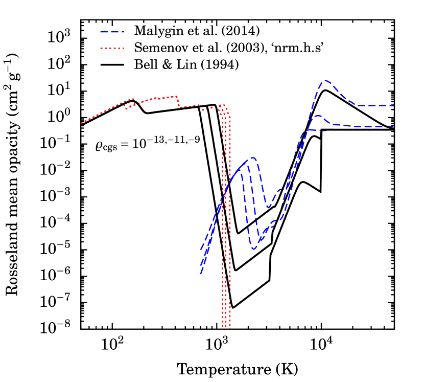
Figure 1: Gas, dust, and total Rosseland mean opacities from Malygin et al. (2014), BL94, and Semenov et al. (2003). Three densities are shown: $\varrho=10^{-13,-11,-9}$ g cm^-3. For the Semenov et al. (2003) opacities, we use their ‘nrm.h.s’ model, with dust grains made of ‘normal silicates’ ([Fe/(Fe+Mg$)]=0.4$) as homegeneous spheres. The Malygin et al. (2014) opacities are kept constant above the table limit of $T=2\times 10^{4}$ K.

Note that the Bell & Lin (1994) lacks water opacity lines just above the dust destruction temperatures (M. Malygin, priv. comm.; see also Figure 1 of Arras & Bildsten, 2006); as a consequence, their opacities reach down to ${\kappa_{\textnormal{R}}}\sim 10^{-6}$ cm² g^-1 for $\rho=10^{-11}$ g cm^-3, where ${\kappa_{\textnormal{R}}}$ is the Rosseland mean, some four orders of magnitude smaller than in more recent calculations (Freedman et al., 2008; Malygin et al., 2014).

Figure 4 shows that for low masses and accretion rates, the shock temperature should be ${T_{\textnormal{s}}}\lesssim 1500$ K, in which case the dust is not destroyed and the opacity is relatively high. When higher temperatures are reached, the opacity is lower by orders of magnitude, so that the total (gas and dust) Rosseland opacities range from ${\kappa_{\textnormal{R}}}\sim 10^{-2}$ to 10 cm² g^-1 overall. This provides approximate values when considering constant opacities. Since 1-$T$ requires only the Rosseland mean, the subscript on ${\kappa_{\textnormal{R}}}$ will be dropped hereafter.

2.6 Quantities to be measured

2.6.1 Efficiencies

The main goal of this study is to determine the radiative loss efficiency of the accretion shock. There are several ways of defining this. The classical definition, $\eta^{\rm kin}$, indicates what fraction of the inward-directed kinetic energy flux is converted into a jump in outgoing radiative flux (e.g., Hartmann et al., 1997; Baraffe et al., 2012; Zhu, 2015). This kinetic-energy luminosity is at most

$${L_{\rm acc,~{}max}} =4\pi{R_{\textnormal{p}}}^{2}\frac{1}{2}\varrho v^{3}=\frac{1}{2}{\dot{M}}v^{2}$$ (15)

$$\approx\frac{G{M_{\textnormal{p}}}{\dot{M}}}{{R_{\textnormal{p}}}},$$ (16)

where ${\dot{M}}=4\pi r^{2}\varrho v$ is the mass accretion rate (neglecting the sign of $v$) and the last expression is valid for free fall from a large radius. Therefore, the energy actually radiated away at the shock is written as

$${L_{\rm acc}}=\eta^{\rm kin}\frac{G{M_{\textnormal{p}}}{\dot{M}}}{{R_{\textnormal{p}}}}$$ (17)

and it is usually assumed that $\eta^{\rm kin}=100$ percent (i.e., full loss). This is called ‘cold accretion’. Note that this $\eta^{\rm kin}$ corresponds to the quantity $(1-\eta)$ of Spiegel & Burrows (2012), $\alpha_{\rm h}$ of Mordasini et al. (2012), $(1-\alpha)$ of Hartmann et al. (1997), and $X$ of Commerçon et al. (2011).

We present here and use a second definition based on the total energy available. This efficiency $\eta^{\rm phys}$ measures what fraction of the total energy flowing towards the planet actually remains below the shock, i.e., is absorbed by the embryo:

$$\eta^{\rm phys}\equiv\frac{{\dot{E}}({r_{\rm max}})-{\dot{E}}({r_{\rm shock}}^{-})}{{\dot{E}}({r_{\rm max}})},$$ (18)

where ${r_{\rm shock}}^{-}$ is immediately downstream of the shock and the outer edge of the computation domain ${r_{\rm max}}$ is used as a proxy for the accretion radius ${R_{\textnormal{acc}}}$ corresponding to the location of the nebula. The material-energy flow rate is defined as

$${\dot{E}}(r)\equiv-|{\dot{M}}|\left[{e_{\textnormal{kin}}}(r)+h(r)+\Delta\Phi(r,{r_{\rm shock}})\right],$$ (19)

where ${e_{\textnormal{kin}}}=\frac{1}{2}v^{2}$, ${e_{\textnormal{int}}}$, and $h={e_{\textnormal{int}}}+P/\rho$ are respectively the kinetic energy, internal energy density, and the enthalpy per unit mass and $\Phi$ the external potential. The $\Delta\Phi$ term in Equation (19) accounts for the work done by the potential on the gas down to the shock, with the potential difference from $r_{0}$ to $r$ given by

$$\Delta\Phi(r,r_{0})=-G{M_{\textnormal{p}}}\left(\frac{1}{r}-\frac{1}{r_{0}}\right).$$ (20)

Thus $\eta^{\rm phys}$ measures how much of the incoming energy flow ${\dot{E}}({r_{\rm max}})$ in the gas is still flowing inward once it has passed through the shock; if both are equal (${\dot{E}}({r_{\rm shock}}^{-})={\dot{E}}({r_{\rm max}})$), $\eta^{\rm phys}=0$ and the accretion would be thought of as ‘hot’. If in the other extreme case none of the energy traverses the shock, $\eta^{\rm phys}=100$ percent, implying that the energy must have been entirely converted to outward-traveling radiation. This therefore automatically reflects the fact that the (non-)heating of the planet is determined by the imbalance between the amount of kinetic energy converted to internal energy and the re-emitted radiation.

By energy conservation, the numerator of $\eta^{\rm phys}$ should be equal to the difference ${\dot{E}}({r_{\rm shock}}^{+})-{\dot{E}}({r_{\rm shock}}^{-})$ between the material energy flow rate directly across the shock. This is true for a zero-temperature gas (infinite Mach number), for which the potential energy is entirely converted in kinetic energy by the external potential. For finite temperatures, however, a (small) pressure gradient builds up ahead of the shock; in this case, only part of the change in potential energy serves to increase the kinetic energy, the remainder going into internal energy and thus, outside of phase transitions, into pressure.

Also by energy conservation, $\Delta{\dot{E}}({r_{\rm shock}}^{\pm})$ measured in the shock frame should be equal (up to a sign) to the change in the luminosity $\Delta L$ across the shock. However, in the case that the radiative precursor (Zel’dovich & Raizer, 1967) is contained within the accretion region—roughly the Hill sphere—, it is not true anymore that ${\dot{E}}({r_{\rm shock}}^{+})={\dot{E}}({r_{\rm max}})$. In fact, the luminosity upstream of the precursor can be smaller than downstream (i.e., the planet is invisible, at least in the grey approximation), which would lead to a negative efficiency if using $\Delta L$. Thus, $\Delta{\dot{E}}$ is a more useful numerator because it is intuitive and applicable both when the precursor reaches to ${r_{\rm max}}$ and not.

Note finally that the definition of Equation (18) takes into account the fact that even if the entire kinetic energy is converted to luminosity, the net efficiency can still be zero if this radiation is absorbed by the incoming material. This was seen by Vaytet et al. (2013a) in the case of Larson’s second core and estimated by Baraffe et al. (2012) to be the case at high accretion rates in the context of magnetospheric accretion onto stars.

Thus, we will focus in this study on the efficiencies as defined above: on the classical, ‘kinetic’ efficiency $\eta^{\rm kin}$, which makes a direct statement about the energy conversion at the shock, with $\eta^{\rm kin}<100$ percent for either an isothermal shock at Mach number ${\mathcal{M}}\lesssim 2.5$ (Commerçon et al., 2011) or an non-isothermal shock; and on the ‘physical’ efficiency $\eta^{\rm phys}$, which indicates how much the upstream gas is able to recycle the energy liberated at the shock (Drake, 2006).

2.6.2 Post-shock entropy

The post-shock temperature and thus entropy depend on the thermal profile of the layers below the shock, which are expected to adjust to carry the luminosity from deeper down (Paxton et al., 2013). Since however we do not attempt to predict this luminosity accurately with our set-up of a truncated atmosphere, the reported temperature values will serve only as an indication. Moreover, there is a non-trivial relationship between the post-shock entropy values and their influence on the entropy of the planet’s deep adiabat; in particular, the post-shock material does not simply set, weigthed by mass, the interior entropy. This question is the subject of separate studies (Berardo et al., 2016, Marleau et al., in prep.), which however require the obtained post-shock entropies as boundary conditions.

3 Results: radial profiles and efficiencies

We have performed a large number of simulations, varying physical parameters (mass, radius, accretion rate) but also computational or numerical settings (technique for accreting gas into the domain, outer temperature boundary condition, resolution, Courant number, etc.). For the latter, we select the most stable set-up (as described in Section 2.2 above), and present results for a typical combination relevant to core accretion formation calculations (Bodenheimer et al., 2000; Mordasini et al., 2012). We look at the properties of the accretion shock for ${M_{\textnormal{p}}}=1.3~{}{M_{\textnormal{J}}}$, ${\dot{M}}=10^{-2}~{}{M_{\oplus}}\,\rm{yr}^{-1}$, and ${r_{\rm shock}}\approx 1.8~{}{R_{\textnormal{J}}}$. The Bondi, Hill, and resulting accretion radius according to Equation (1) are ${R_{\textnormal{Bondi}}}\approx 4200~{}{R_{\textnormal{J}}}$, ${R_{\textnormal{Hill}}}\approx 800~{}{R_{\textnormal{J}}}$, and ${R_{\textnormal{acc}}}\approx 250~{}{R_{\textnormal{J}}}$ (for ${T_{\textnormal{neb}}}=150$ K and a solar-mass star, which however does not affect ${R_{\textnormal{acc}}}$ strongly). Figure 2 shows the detailed structure of the accretion flow near the shock for $\kappa=10^{-2}$ and 1 cm² g^-1, as well as with the Bell & Lin (1994) opacities. For the EOS, we consider a hydrogen–helium mixture with a helium mass fraction $Y=0.25$ and cases where hydrogen is everywhere molecular ($\mu=2.353$, $\gamma=1.44$) or atomic ($\mu=1.23$, $\gamma=1.1$). The radial structures are as expected and show a number of typical features, which we discuss in the following.

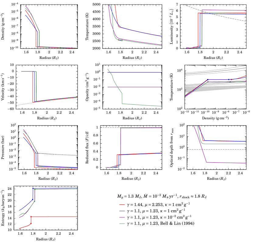
Figure 2: Detailed shock profiles for simulations with ${M_{\textnormal{p}}}=1.3~{}{M_{\textnormal{J}}}$, ${r_{\rm shock}}\approx 1.8~{}{R_{\textnormal{J}}}$, and ${\dot{M}}=10^{-2}~{}{M_{\oplus}}\,\rm{yr}^{-1}$ using a constant equation of state and constant opacities or the Bell & Lin (1994) opacities (see legend). The simulation grids extend to 0.7 of the accretion radius ${R_{\textnormal{acc}}}\approx 250~{}{R_{\textnormal{J}}}$ but only the inner region is shown. The axis labels describe the quantities shown, and only a few comments are needed: The temperature panel also shows the lower bound estimate of Equation (28b; filled dots); in the luminosity panel, the maximal accretion luminosity ${L_{\rm acc,~{}max}}(r)=\frac{1}{2}{\dot{M}}v(r)^{2}\approx G{M_{\textnormal{p}}}{\dot{M}}/r$ is shown at every radius (gray dashed curve); the velocity panel also displays the free-fall velocity from ${R_{\textnormal{acc}}}$ (the same for all simulations; grey dotted line); in the opacity panel, simulations with constant opacity overlap; in the temperature–density phase diagram, the solid dots mark the up- and downstream conditions of shock, the solid lines show contours of 10, 50, and 90 percent atomic hydrogen (relative to the hydrogen species), and the grey region hightlights where the dust is being destroyed, with $\kappa\sim 1$ cm² g^-1 below and $\kappa\sim 10^{-6}$–10^-3 cm² g^-1 above; the pressure panel also displays the ram pressure $P_{\rm ram}=\rho v^{2}$, the same for all simulations (dashed curve); and the entropy is computed self-consistently from Equation (29).

3.1 Density, velocity, and pressure

The density and velocity reveal gas almost exactly free-falling onto a nearly hydrostatic atmosphere abruptly cut off at the shock. The mass in the total domain, dominated by the post-shock region, is typically $\Delta M\sim 10^{-4}~{}{M_{\oplus}}$, making perfectly justified the neglect of the self-gravity of the gas. The density jumps at the shock by a factor $\rho_{2}/\rho_{1}\sim 200$, where $\rho_{2}$ and $\rho_{1}$ are the post- and pre-shock density. Thanks to the transport of energy by radiation, this is a much larger compression than the infinite-Mach number limit for a hydrodynamical shock, where $\rho_{2}/\rho_{1}=(\gamma+1)/(\gamma-1)\approx 4$ to 20 for $\gamma=\frac{5}{3}$ to 1.1 (e.g., Mihalas & Mihalas, 1984; Commerçon et al., 2011). As it falls deeper in the potential well of the planet, the gas slows down to slightly sub-free-fall speeds due to the pressure gradient caused by the increasing temperature and density.

The post-shock pressure is given very accurately by the ram pressure of the incoming gas,

$$P_{\rm post}=P_{\rm ram}=\varrho v^{2}.$$ (21)

This differs slightly from the strong-shock (high-Mach-number), non-radiating case where $P_{\rm post}=2/(\gamma+1)\varrho v^{2}$ (Drake, 2006, his Equation 4.18), as we verified with a simulation using a higher $\gamma=5/3$ to increase the difference.

3.2 Optical depth, reduced flux, and radiation regime

We begin by discussing the reduced flux. The reduced flux

$${f_{\textnormal{red}}}\equiv{F_{\rm rad}}/(c{E_{\textnormal{rad}}})$$ (22)

is a local measure of the extent to which radiation is streaming freely (${f_{\textnormal{red}}}\rightarrow 1$) or diffusing (${f_{\textnormal{red}}}\rightarrow 0$). This is thus the more correct, physical measure of what is often loosely termed the optical depth, as discussed below. The reduced flux, radiation quantity $R$, and flux limiter $\lambda$ are related in general by ${f_{\textnormal{red}}}=\lambda(R)R$. Note that the effective speed of propagation of the photons is ${c_{\textnormal{eff}}}={f_{\textnormal{red}}}c$.

Next, we consider the optical depth. For a free-fall profile with ${R_{\textnormal{acc}}}\gg{r_{\rm shock}}$ (so that $\rho\propto r^{-3/2}$) and a radially sufficiently constant opacity ($\kappa\propto r^{\alpha}$ with $|\alpha|\ll\frac{1}{2}$), the optical depth to the shock is

$$\Delta\tau =\int_{r_{\rm shock}}^{\infty}\kappa(r)\rho(r){\rm d}r$$ (23a)

$$=2\kappa\rho{r_{\rm shock}}~{}~{}~{}\textnormal{(const.~{}$\kappa$)},$$ (23b)

where $\kappa\rho$ is evaluated at the shock. For the data of Figure 2, $\rho=1.5\times 10^{-10}$ g cm^-3 upstream of the shock, so that $\Delta\tau=3.9\left(\kappa/1~{}\mbox{cm${}^{2}$\,g${}^{-1}$}\right)$. This agrees very well with the actual optical depths (measured from ${r_{\rm max}}=0.7{R_{\textnormal{acc}}}\approx 250~{}{R_{\textnormal{J}}}$) in the constant-opacity cases. For the simulation with the Bell & Lin (1994) opacities, the estimate is moderately accurate, if one takes for $\kappa$ not the actual pre-shock value ($\kappa\sim 10^{-5}$ cm² g^-1, set by the gas) but rather a typical value ($\kappa\sim 1$ cm² g^-1) in the outer regions ($r\gtrsim 40~{}{R_{\textnormal{J}}}$), where the dust is not destroyed. Also for non-constant opacities, then, the optical depth to the shock will be roughly given by

$$\Delta\tau\sim 3\left(\frac{\kappa}{1~{}\mbox{cm${}^{2}$\,g${}^{-1}$}}\right) \left(\frac{{\dot{M}}}{10^{-2}~{}{M_{\oplus}}\,{\rm yr}^{-1}}\right)$$

$$\times\sqrt{\left(\frac{1~{}{M_{\textnormal{J}}}}{{M_{\textnormal{p}}}}\right)\left(\frac{2~{}{R_{\textnormal{J}}}}{{r_{\rm shock}}}\right)},$$ (24)

using that ${\dot{M}}=4\pi r^{2}\rho v$. Since the nebula should always be at temperatures lower than the dust destruction temperature ${T_{\textnormal{dest}}}\approx 1500$ K, the high opacity of the dust will always contribute to the optical depth. Therefore, independently of whether dust is destroyed in the inner parts of the flow, close to the shock, the opacity to insert in Equation (24) should be of order $\kappa\sim 1$ cm² g^-1.

Secondly, writing ${E_{\textnormal{rad}}}={F_{\rm rad}}/(c{f_{\textnormal{red}}})\propto L/(r^{2}{f_{\textnormal{red}}})$, it is clear that when $L/{f_{\textnormal{red}}}$ is locally spatially constant ($L/{f_{\textnormal{red}}}\propto r^{\beta}$ with $|\beta|\ll 2$), the radiation quantity $R=1/(\kappa\rho)\left|\partial\ln{E_{\textnormal{rad}}}/\partial r\right|$ is given by $R\approx 2/(\kappa\rho r)$ where $\kappa\rho$ and $r$ are evaluated locally. This result applies in general, independently of the radiation regime (diffusion or free streaming).

Combining these observations leads to the result that, in the case of constant opacity and $L/{f_{\textnormal{red}}}$, the reduced flux upstream of the shock is

$${f_{\textnormal{red}}}({r_{\rm shock}}^{+}) =\lambda\left(\frac{4}{\Delta\tau}\right)\times\frac{4}{\Delta\tau}$$ (25a)

$$\approx\left(\frac{3}{4}\Delta\tau+1\right)^{-1},$$ (25b)

where the second line would be an equality for the simple flux limiter $\lambda=1/(3+R)$ (LeBlanc & Wilson, 1970; Levermore, 1984; Ensman, 1994). We will return to this result in Section 3.3. For a non-constant opacity, Equation (25) provides in fact an approximate lower bound of ${f_{\textnormal{red}}}({r_{\rm shock}}^{+})$ given $\Delta\tau$ or vice versa: indeed, a low opacity in front of the shock will drive down ${f_{\textnormal{red}}}$ (compared to the prediction of Equation (25)) but without decreasing much the total optical depth. This highlights the conceptual independence between the (non-local) optical depth and the (local) radiation transport regime (free-streaming or diffusion).

The optical depths from the shock out to ${r_{\rm max}}\approx{R_{\textnormal{acc}}}$ are $\Delta\tau\approx 2$–5 for all except the $\kappa=10^{-2}$ cm² g^-1 simulation, which has $\Delta\tau\approx 3\times 10^{-2}$. (A comparison run with the dust opacities of Semenov et al. (2003) and the gas opacities of Malygin et al. (2014) yielded very similar profiles and optical depths.) In the $\kappa\neq 10^{-2}$ cm² g^-1 simulations, the shock would therefore be called ‘optically thick’. However, the effective speed of light ${c_{\textnormal{eff}}}={f_{\textnormal{red}}}c\gtrsim 0.3c$ throughout the flow (see below), which is still orders of magnitude larger than the gas flow speed $v\sim 10^{-4}c$. This is the regime Mihalas & Mihalas (1984) term ‘static diffusion’. Therefore, the radiation is able to diffuse into the incoming gas, heating it up out to the edge of the computation grid, near the accretion radius. In other words, the shock precursor is larger than the Hill radius, which implies that the radiation should be able to escape from the system to at least the local disk. In this sense, the shock for these parameter values is an optically thick–thin shock (down- and upstream, respectively) in the classification of Drake (2006). That despite the somewhat high optical depth the shock is not equivalent to a hydrodynamical shock is already hinted at by the large compression ratio pointed out in Section 3.1.

3.3 Temperature

3.3.1 Shock temperature

For all choices of $\kappa$ and the EOS ($\gamma$, $\mu$), the temperatures immediately up- and downstream of the shock are essentially equal, i.e., there is no jump in the temperature. This is thus a supercritical shock (Zel’dovich & Raizer, 1967), in which the downstream gas is able to pre-heat the incoming gas up to the post-shock temperature. Note that the 1-$T$ approach to the radiation transport used here cannot reveal the Zel’dovich spike expected in the gas temperature. This feature of radiation-hydrodynamical shocks consists of a sharp increase of the gas temperature immediately behind the shock, followed by a quick decrease in a ‘radiative relaxion region’, while the radiation temperature remains essentially constant (Zel’dovich & Raizer, 1967; Mihalas & Mihalas, 1984; Stahler et al., 1980; see Drake 2007 and Vaytet et al. 2013b for a more detailed description). However, this is not of concern since this spike is very thin both spatially (physically, a few molecular mean free paths, broadened in simulations to a few grid cells; e.g., Ensman, 1994; Vaytet et al., 2013b; Marleau et al. in prep.) and in optical depth, and below the Zel’dovich spike, the matter and radiation equilibrate again. Therefore, the Zel’dovich spike should affect neither the post-shock temperature or entropy nor the shock efficiency. A possible disequilibrium in temperatures just upstream of the shock will be explored in a forthcoming publication.

We find shock temperatures of ${T_{\rm shock}}\approx 2500$ K for the cases with a low pre-shock opacity ($\kappa=10^{-2}$ cm² g^-1 or with Bell & Lin (1994)), but ${T_{\rm shock}}\approx 3500$ K for the other two cases, both with $\kappa=1$ cm² g^-1. These temperature values (and their relatively large difference of 1000 K) can be understood from an analytical estimate, presented next. Firstly, one can always write

$$F({r_{\rm shock}}^{+})=F({r_{\rm shock}}^{-})+\eta^{\rm kin}\frac{1}{2}\rho{v_{\rm shock}}^{3},$$ (26)

where here $\rho$ is the density just ahead of the shock, ${v_{\rm shock}}$ is the velocity at the same location, and $\eta^{\rm kin}$ is the ‘kinetic-energy loss efficiency’, discussed in Section 3.6. In general, the flux on either side of the flux is $F({r_{\rm shock}}^{\pm})={f_{\textnormal{red}}}^{\pm}caT^{4}({r_{\rm shock}}^{\pm})$, where ${f_{\textnormal{red}}}^{\pm}\equiv{f_{\textnormal{red}}}({r_{\rm shock}}^{\pm})$ and $a$ is the radiation constant, related to the Stefan–Boltzmann constant ${\sigma}$ by $ac=4{\sigma}$. Note that here ${f_{\textnormal{red}}}={F_{\rm rad}}/c{E_{\textnormal{rad}}}$ should be negative (one usually implicitly takes the norm) if the downstream radiation is flowing inward (${F_{\rm rad}}<0$). For an isothermal shock at ${T_{\rm shock}}$, Equation (26) then implies that

$${\sigma}{T_{\rm shock}}^{4}=\frac{\eta^{\rm kin}}{4\Delta{f_{\textnormal{red}}}}\frac{\rho{v_{\rm shock}}^{3}}{2},$$ (27)

where $\Delta{f_{\textnormal{red}}}\equiv{f_{\textnormal{red}}}^{+}-{f_{\textnormal{red}}}^{-}$. Combining with Equations (24) and (25) yields the estimates for an isothermal shock

$${T_{\rm shock}}(\Delta\tau\ll 1)\approx ~{}2315~{}{\rm K}\left(\frac{{r_{\rm shock}}}{2~{}{R_{\textnormal{J}}}}\right)^{-3/4}$$

$$\left(\frac{{\dot{M}}}{10^{-2}~{}{M_{\oplus}}\,{\rm yr}^{-1}}\right)^{1/4}\left(\frac{M}{1~{}{M_{\textnormal{J}}}}\right)^{1/4}$$ (28a)

$${T_{\rm shock}}(\Delta\tau\gg 1)\approx ~{}2710~{}{\rm K}\left(\frac{{r_{\rm shock}}}{2~{}{R_{\textnormal{J}}}}\right)^{7/8}\left(\frac{\kappa}{1~{}{\rm cm}^{2}\,{\rm g}^{-1}}\right)^{1/4}$$

$$\left(\frac{{\dot{M}}}{10^{-2}~{}{M_{\oplus}}\,{\rm yr}^{-1}}\right)^{1/2}\left(\frac{M}{1~{}{M_{\textnormal{J}}}}\right)^{1/8},$$ (28b)

where a $\left({\eta^{\rm kin}}\right)^{1/4}$ factor was left out on the right-hand sides since we find it is $\approx 1$ (see Section 3.6). The first expression used that, by Equation (25), $\Delta\tau\ll 1$ implies ${f_{\textnormal{red}}}^{+}\approx 1$, and further took ${f_{\textnormal{red}}}^{-}\ll{f_{\textnormal{red}}}^{+}$. The second case is somewhat crude for non-constant opacities. This assumes a constant luminosity in the shock’s near upstream vicinity. Since the post-shock region is very dense, ${f_{\textnormal{red}}}^{-}$ is small; this is equivalent to neglecting the downstream luminosity, which is related in a non-trivial way to the interior luminosity of the planet (Berardo et al., 2016; Marleau et al., in prep.).

The filled circles in Figure 2 show the lower bound of Equation (28b). The simulations with a low pre-shock opacity ($\kappa=10^{-2}$ cm² g^-1 or with Bell & Lin (1994)) have ${f_{\textnormal{red}}}\approx 1$ upstream of the shock and indeed have a temperature given by Equation (28b), whereas in the other cases a higher temperature is needed to carry a similar luminosity. The difference is quite large and nearly 1000 K. One way of thinking about this is that the effective speed of light is lower than $c$, so that ${E_{\textnormal{rad}}}$ must increase in order to reach the same ${F_{\rm rad}}=c_{\rm eff}{E_{\textnormal{rad}}}$.

Interestingly, the molecular- and atomic-hydrogen cases lead to a very similar temperature ${T_{\rm shock}}=3500$ K. The phase diagram indicates that the atomic-hydrogen simulation with $\kappa=1$ cm² g^-1 is self-consistent, but that the case with atomic hydrogen and detailed opacities leads to temperatures and densities where the dissociation process (and thus a varying $\mu$ and $\gamma$) would be important. One can already anticipate the result that, for an isothermal shock, the hydrogen should recombine in part through the shock (Marleau et al., in prep.) since at fixed temperature the abundance of H₂ increases with density.

Note that Stahler et al. (1980, their Equation 24) present an estimate similar to Equation (27) in the context of stellar accretion. Their assumptions about the reprocessing of shock photons imply that, when ${F_{\rm rad}}({r_{\rm shock}}^{-})\ll{F_{\rm rad}}({r_{\rm shock}}^{+})$ and neglecting their $T_{d}$ term, $\Delta{f_{\textnormal{red}}}\approx{f_{\textnormal{red}}}^{+}\approx 1/3$ automatically. Commerçon et al. (2011, their Equation 22 or 53) give a formula similar to Equation (27) in the limiting case $\eta^{\rm kin}=1$ but do not include the factor $1/(4\Delta{f_{\textnormal{red}}})$. This is because they equate the temperature at the shock with the effective temperature needed to radiate away the kinetic energy, increasing the temperature estimate by $\approx 40$ % (a factor $4^{1/4}\approx 1.4$), or $\approx 1200$ K for ${T_{\textnormal{s}}}\approx 3000$ K.

3.3.2 Temperature profile

Equation (22) implies that, if the luminosity and the reduced flux are radially roughly constant, $T\propto r^{-1/2}$ since $L=4\pi r^{2}{F_{\rm rad}}$, independently of the optical depth to the shock. This is the case for the constant-$\kappa$ simulations but not so for the tabulated opacities (at larger radial distances than shown).

Note that if the temperature increased solely due to adiabatic compression, i.e., at constant entropy in the absence of radiation transport, we would have $T\propto\varrho^{\gamma-1}\propto r^{-1.5(\gamma-1)}$, i.e., $T\propto r^{-0.15}$ or $T\propto r^{-0.66}$ for $\gamma=1.1$ or $1.44$, respectively. Thus, when $T\propto r^{-1/2}$, entropy decreases inward if $\gamma>4/3\approx 1.33$.

3.4 Entropy

To compute the entropy, we use the Sackur–Tetrode equation (e.g., Marleau & Cumming, 2014; Berardo et al., 2016, and references therein) for an ideal gas composed of H₂ and He or H and He:

$$S_{\textrm{H}_{2}\mbox{--}\textrm{He}}= \,8.80+3.38\log_{10}\left(\frac{T}{1000~{}{\rm K}}\right)$$

$$-1.01\log_{10}\left({P\over 1\ {\rm bar}}\right),$$ (29a)

$$S_{\textrm{H}\mbox{--}\textrm{He}}= \,13.47+4.68\log_{10}\left(\frac{T}{1000~{}{\rm K}}\right)$$

$$-1.87\log_{10}\left({P\over 1\ {\rm bar}}\right),$$ (29b)

respectively, using $Y=0.243$, and where the entropies are in units of Boltzmann’s constant per baryon, ${k_{\textnormal{B}}}/\mbox{baryon}$. In Figure 2, we see that the entropy decreases across the shock by $|\Delta S|\approx 2.5$ and 4.0 ${k_{\textnormal{B}}}/\mbox{baryon}$ for the molecular and atomic case, respectively. (In general but for constant $\gamma$ and $\mu$, the jump in entropy at an isothermal shock is $\Delta S=-2.303/\mu\times\log_{10}(\gamma{\mathcal{M}}^{2})$ in units of ${k_{\textnormal{B}}}/\mbox{baryon}$.) That the entropy decreases through this shock is actually in agreement with the statement that entropy increases across a hydrodynamical shock. Indeed, once it arrives at the radiative shock found here, the gas has already seen its entropy increase from the value far outside of the precursor. (In the case that the precursor is larger than the simulation domain, as applies for these simulations, this ‘far-field’ value cannot be obtained directly. However, already at ${r_{\rm max}}$ is the entropy much lower than downstream of the shock.) Thus the radiative shock which is the subject of this work can be thought as being embedded in a usual hydrodynamical shock, a ‘shock within a shock’ (Mihalas & Mihalas, 1984), or a hydrodynamical shock as being a radiative shock with an infinitely or unresolved thin precursor. Separate test simulations with extremely high opacity values ($\kappa=10^{2}$ cm² g^-1), such that the precursor is contained in the simulation domain, confirm that the post-shock entropy is higher than the entropy far away from the shock.

The post-shock entropies are respectively $S\approx 12$ and 20 ${k_{\textnormal{B}}}/\mbox{baryon}$ for the molecular and atomic cases. Compared to the range of entropies seen for cold starts to hot starts ($S\approx 8$–14 ${k_{\textnormal{B}}}/\mbox{baryon}$; Marley et al., 2007; Spiegel & Burrows, 2012; Mordasini, 2013), this is an extremely large difference, which is due mostly to the different mean molecular weights. Moreover, it highlights the importance of using a self-consistent EOS which follows in particular the dissociation of hydrogen. However, the entropy values do not depend sensitively on the precise opacity (see Figure 2).

Finally, it is important to remember that these entropy values are meant to be rather indicative at this stage. First of all, they are not entirely self-consistent with the probable state of the hydrogen in all parts of the domain (see the phase diagram in Figure 2). Second of all, what they actually imply for the post-formation entropy needs to be worked out separately, with a study of the post-shock settling region and its coupling to the planet interior (Berardo et al., 2016, Marleau et al., in prep.).

3.5 Luminosity

The luminosity increases from the imposed $L=0$ value at ${r_{\rm min}}$ to the shock where it jumps by a finite amount $\Delta L$, then decreasing with radius. The value of $L$ downstream of the shock reflects in part the cooling of the layers below it, and is set in reality also by (inefficient) convective energy transport, which we do not attempt to include in these simulations. Thus the post-shock gas will probably have a different thermal history than if the layers were allowed to sink further down into the planet instead of stopping at most at ${r_{\rm min}}$. Nevertheless, the obtained immediate post-shock luminosities are roughly ${L_{\rm downstr}}\approx 3\times 10^{-4}~{}{L_{\odot}}$ and thus have values comparable to the (rough) internal luminosities of accreting planets (Mordasini et al., submitted). Therefore, the inclusion of convection or similar changes to the temperature structure should not lead to very different values for the post-shock region.

A general feature of these shock simulations is that $L$ decreases radially outward. This is not due to absorption of the light with optical depth according to $L\propto\exp{(-\Delta\tau)}$, as one might naively expect, but rather reflects energy conservation. To derive this, we start with the total energy equation (e.g., Kuiper et al., 2010),

$$\frac{d{E_{\textnormal{tot}}}}{dt}+\nabla\cdot([{E_{\textnormal{kin}}}+H]v+{F_{\rm rad}})=\varrho v\cdot g,$$ (30)

where the total energy volume density is ${E_{\textnormal{tot}}}={E_{\textnormal{kin}}}+H$, with ${E_{\textnormal{kin}}}=\frac{1}{2}\rho v^{2}$, and the enthalpy is $H={E_{\textnormal{int}}}+P$ for an internal energy density ${E_{\textnormal{int}}}$. For a constant EOS, ${E_{\textnormal{int}}}=\rho{c_{\textnormal{v}}}T=\rho/(\gamma-1)\times{k_{\textnormal{B}}}T/(\mu{m_{\textnormal{H}}})=1/(\gamma-1)\times P$, where ${c_{\textnormal{v}}}$ is the heat capacity. It is easy to verify that the thermal timescales are much shorter than the dynamical timescales, so that the flow is in steady state and the time derivative $d{E_{\textnormal{tot}}}/dt$ can be neglected. Also, ${\dot{M}}$ is constant radially. Remembering that $\nabla\cdot F=1/r^{2}d/dr(r^{2}F)$ for a vector $F$, Equation (30) becomes

$$\frac{dL}{dr}={\dot{M}}\frac{dh}{dr}+{\dot{M}}\frac{d}{dr}\left(\frac{1}{2}v^{2}-\frac{G{M_{\textnormal{p}}}}{r}\right),$$ (31)

where $h=H/\rho$ is the specific enthalpy per mass and is $h=\gamma/(\gamma-1){k_{\textnormal{B}}}T/(\mu{m_{\textnormal{H}}})$ for a constant EOS. The accretion rate ${\dot{M}}$ was taken to be positive here, i.e., ${\dot{M}}=|4\pi r^{2}\rho v|$, and one can trivially replace $G{M_{\textnormal{p}}}/r$ by $G{M_{\textnormal{p}}}\left(1/r-1/{R_{\textnormal{acc}}}\right)$. If the second term on the righthand side of Equation (31) is small, Equation (31) shows that the radial decrease in $L$ is mostly due to the inward increase in enthalpy. Therefore, it is not an explicit function of the optical depth, although $T(r)$ and thus $h(T)$ are indirectly set by the opacity. Note that this derivation is valid for a general EOS (with variable effective $\gamma$) and also does not depend on the opacity being constant.

Equation (31) can be integrated to yield, when the second term on the righthand side of Equation (31) is negligible,

$$L(r)-{L_{\rm downstr}}=\Delta L({r_{\rm shock}})\left[1-\frac{{\dot{M}}\Delta h(r)}{\Delta L({r_{\rm shock}})}\right],$$ (32)

where $\Delta L({r_{\rm shock}})=\eta^{\rm kin}{L_{\rm acc,~{}max}}$ is the jump in luminosity at the shock, and $\Delta h(r)\equiv h({r_{\rm shock}})-h(r)$ is the change in enthalpy relative to the shock, with $\Delta h>0$ for outwards decreasing enthalpy. This result seems plausible: the inward enthalpy flux is comparable to the outward radiation flux only when the infalling gas absorbs a significant fraction of the radiation and thus decreases $L$. The maximal drop in luminosity occurs for $h({r_{\rm max}})\ll h({r_{\rm shock}})$, i.e., when the effective nebula temperature ${T_{\textnormal{neb}}}\ll{T_{\rm shock}}$. This leads to $L({r_{\rm max}})-L({r_{\rm shock}}^{+})=-{\dot{M}}h({T_{\rm shock}})$.

3.6 Efficiencies

Next we show in Figure 3 the main result for the examples of Figure 2, the loss efficiency $\eta^{\rm phys}$ of the accretion shock. We recall that $\eta^{\rm phys}=0$ would correspond to all the kinetic energy of the gas being absorbed by the planet and the gas being accreted, while $\eta^{\rm phys}=100$ percent would correspond to the entire kinetic energy being radiated away when going out to the accretion radius ${R_{\textnormal{acc}}}$, roughly the Hill sphere (here approximated by the outer radius near ${R_{\textnormal{acc}}}$). Contrary to $\eta^{\rm kin}$, $\eta^{\rm phys}$ takes into account the energy recycling which occurs due to the incoming gas absorbing the radiation liberated at the shock (see Equation (18) and the discussion below Equation (20)). We find that they are $\eta^{\rm phys}\approx 85$ percent for the atomic-hydrogen cases with different opacities, and $\eta^{\rm phys}\approx 95$ percent for the molecular case. Thus, a fraction $1-\eta^{\rm phys}\approx 5$–15 percent of the total incoming energy is added to the planet. How significant this is for the energy budget of the planet can be assessed by comparing $(1-\eta^{\rm phys}){\dot{E}}({r_{\rm max}})$ to the internal luminosity of the planet. For these simulations, both are typically of the same order of magnitude, implying that the accreting gas is able to heat the downstream region. As mentioned above, how this then affects the entropy and luminosity of the planet and their evolution will have to be studied separately.

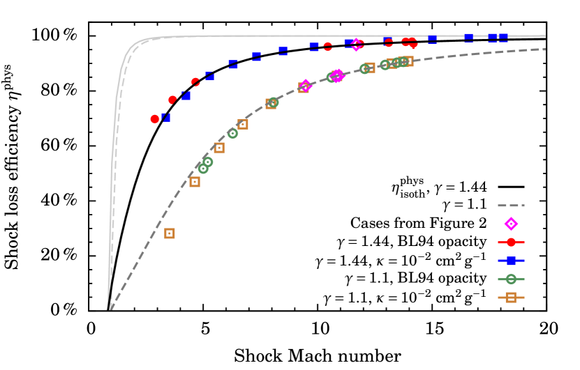
Figure 3: Physical loss efficiency $\eta^{\rm phys}$ of the radiative accretion shock (see Equation (18)). The limit $\eta^{\rm phys}=0$ corresponds to all the incoming energy being absorbed (no loss), while $\eta^{\rm phys}=100$ percent means that the kinetic energy of the gas entirely leaves the accretion flow onto the planet; see Section 2.6.1. The diamonds display the efficiency for the cases shown in Figure 2. The other points come from considering a range of accretion rates ${\dot{M}}=10^{-5}$–$10^{-2}~{}{M_{\oplus}}\,{\rm yr}^{-1}$, masses ${M_{\textnormal{p}}}\approx 0.3$–10 ${M_{\textnormal{J}}}$, and shock locations ${r_{\rm shock}}\approx 1$–$20~{}{R_{\textnormal{J}}}$. Both constant and tabulated opacities are used as indicated in the legend. The last four groups of points (see legend) all take $\mu=2.353$. The results match the analytical result for an isothermal shock at the measured Mach number (Equation (34, from Commerçon et al., 2011), for $\gamma=1.44$ and $\gamma=1.1$ (solid black and dashed dark gray curves, respectively). Theoretical curves for the ‘kinetic efficiency’ $\eta^{\rm kin}_{\textrm{isoth}}$ for an isothermal shock are shown for comparison (pale grey curves).

We show also the efficiencies from simulations covering a range of accretion rates ${\dot{M}}=10^{-5}$–$10^{-2}~{}{M_{\oplus}}\,{\rm yr}^{-1}$, masses ${M_{\textnormal{p}}}\approx 0.3$–10 ${M_{\textnormal{J}}}$, and shock locations ${r_{\rm shock}}\approx 1$–$20~{}{R_{\textnormal{J}}}$, and varying again the opacity. At the largest radii, efficiencies down to almost 20 percent are reached, and to 99 percent at the other extreme.

By contrast, the ‘kinetic efficiency’ is $\eta^{\rm kin}\approx 100$ percent (up to the numerical accuracy of the code given the resolution) for all simulations shown in Figure 3, with $(1-\eta^{\rm kin}){E_{\textnormal{tot}}}$ smaller by orders of magnitude than ${L_{\textnormal{p}}}$. In other words, the entire kinetic energy is converted to an immediate jump in the luminosity as the gas is brought to subsonic speeds through the shock. However, a significant fraction does get reabsorbed in the accretion flow, leading to the lower $\eta^{\rm phys}$ values. Nevertheless, we find generally that the precursor is greater than the accretion radius, which is of order of the Hill radius. The optical depths from the shock to the Hill sphere are at most $\Delta\tau\sim 30$, and using a variable equation of state (which would yield other temperatures) should not change this significantly. We therefore expect the radiation to always be able to escape from the shock to the local disk (the nebula).

These numerical results can be compared to analytical theory for radiative shocks. Drake (2006, his equation 7.82) derived that the kinetic efficiency of a shock in which radiation pressure is negligible is in general given by

$$\eta^{\rm kin}\equiv\frac{\Delta F}{\frac{1}{2}\varrho_{-}{v_{-}}^{3}}=1+\frac{2}{(\gamma-1){{\mathcal{M}}}^{2}}\frac{\mathfrak{r}-1}{\mathfrak{r}}+\frac{\gamma+1}{\gamma-1}\frac{1}{\mathfrak{r}^{2}}.$$ (33)

where $\mathfrak{r}\equiv\rho_{2}/\rho_{1}$ is the ratio of the post-shock to the pre-shock density. For isothermal shocks (as we find here), $\mathfrak{r}=\gamma{\mathcal{M}}^{2}$, and Commerçon et al. (2011) show that the efficiency is then

$$\eta^{\rm kin}_{\textrm{isoth}}=1-\frac{1}{\gamma^{2}{\mathcal{M}}^{4}}.$$ (34)

Thus a higher Mach number leads to a higher fraction of the incoming kinetic energy being converted to radiation for an isothermal shock. Since the total energy flux is

$$\varrho v{e_{\textnormal{tot}}} =\varrho v\left(\frac{1}{2}v^{2}+h\right)$$ (35a)

$$=\frac{1}{2}\varrho v^{3}\left(1+\frac{2}{\gamma-1}\frac{1}{{\mathcal{M}}^{2}}\right),$$ (35b)

we can derive that the physical efficiency, as measured by $\Delta L$ at the shock, is

$$\eta^{\rm phys}_{\textrm{isoth}}=\eta^{\rm kin}_{\textrm{isoth}}\times\left(1+\frac{2}{\gamma-1}\frac{1}{{\mathcal{M}}^{2}}\right)^{-1}.$$ (36)

Therefore, the physical efficiency is lower than the kinetic since the former considers the heating of the radiative precursor. In other words, not all radiation liberated at the shock can leave the planet, and therefore gets incorporated in the planet’s entropy. Note that naively, one might expect in strongly supersonic flows (${\mathcal{M}}=v/{c_{\rm s}}\gg 1$) the internal energy (measured by ${c_{\rm s}}^{2}$) to be negligible compared to the kinetic energy (measured by $v^{2}$), but the $2/(\gamma-1)$ factor can make this assumption cruder than expected, especially for low $\gamma$ values; for instance, when $\gamma=1.1$ and even with a high Mach number ${\mathcal{M}}=10$, the factor $2/{\mathcal{M}}^{2}(\gamma-1)$ is $0.2$, i.e., a 20 per cent contribution.

The Mach numbers range from ${\mathcal{M}}\approx 3$–20, and the $\eta^{\rm phys}_{\textrm{isoth}}$ curve is compared to the data in Figure 3 for $\gamma=1.1$ and $\gamma=1.44$. The agreement is excellent. The deviation from the theoretical curve, seen for a few simulations, is possibly due to small measurement errors related to the identification of the shock region, and to inaccuracies in the measurement of the velocity at which the shock is spreading; this speed becomes somewhat important (at the several-percent level) at low Mach numbers. However, the overall agreement is excellent, independent of the opacity and optical depth in the flow (not shown).

At least for the constant EOS used here, these simulations and other tests indicate that extreme parameter values (e.g., ${\dot{M}}>10^{-1}~{}{M_{\oplus}}\,{\rm yr}^{-1}$ or $\kappa>100$ cm² g^-1) would be needed to obtain a shock with a Mach number ${\mathcal{M}}\lesssim 2$, in which $\eta^{\rm kin}$ would clearly be lower than 100 percent. Note that, while ${v_{\textnormal{ff}}}\propto\sqrt{{M_{\textnormal{p}}}}$, very small masses are not sufficient to obtain a lower Mach number since ${\mathcal{M}}\propto v/\sqrt{T}$; at lower masses, the temperature in the pre-shock region too is smaller, which does not let ${\mathcal{M}}$ get much lower than about 3.

4 Discussion and Summary

We have studied spherically symmetric gas accretion onto a gas giant during the detached runaway phase, when the gas falls freely from the accretion radius (of order of the Hill radius) onto the planet, where it shocks. We determine the radiative efficiency of the shock at the planet’s surface and argue that this should be defined with the total incoming energy flux, i.e., taking both the kinetic but also the internal energy into account. Even if, at a Mach number ${\mathcal{M}}=4$, an isothermal shock converts 100 percent of the incoming kinetic energy into radiation, only 77 percent (40 percent) for $\gamma=1.44$ ($\gamma=1.1$) ultimately escape, with 23 percent (60 percent) absorbed by the infalling gas and therefore reaccreted to the system. This efficiency has direct observational consequences as it controls the amount of radiation which leaves the planet and is possibly observable. The efficiency is also important since the complementary fraction is carried through the shock into the settling region, where the gas is being incorporated to the planet. To the best of our knowledge, the energetics of the shock have not yet been studied in detail as we have done, yet are thought to be key in determining the post-formation thermal state of gas giants, with several orders of magnitude of difference in the resulting luminosity between the two extreme cases, hot and cold starts.

We have considered both constant and tabulated opacities (Bell & Lin, 1994) but have only used a constant equation of state to concentrate on the shock physics. Therefore, the numerical results are rather illustrative in a quantitative sense, but the qualitative behavior of the radial profiles and the derived results revealed a number of interesting features. We find the following:

1. The shock was observed always to be isothermal, which corresponds in the classical terminology to a supercritical shock (Stahler et al., 1980; Mihalas & Mihalas, 1984).

2. The effective speed of light of the escaping photons is always much larger than the gas flow speed, so that the upstream region is in the ‘static diffusion’ regime (Mihalas & Mihalas, 1984).

3. Our radiation-hydrodynamics simulations confirm, over a large range of Mach numbers, the theoretical expression for the efficiency given by Commerçon et al. (2011, our Equation 34).

4. Unrealistically high constant opacity values were separately verified to be needed to cause the luminosity generated at the shock to be completely absorbed in the precursor, ahead of the shock region. For reasonable constant or tabulated opacities, all luminosity profiles are qualitatively similar, decreasing by some amount with increasing distance and with a non-zero value at the outer edge (see last point below). An analytical formula is derived for the drop based on energy conservation and shows that, roughly, the decrease in luminosity is significant only if the incoming gas carries a significant amount of energy compared to the accretion luminosity.

5. We generally find higher shock temperatures then predicted by the usual estimate of the shock temperature, Equation (28b). We show analytically that this is a lower bound. The shock temperature being higher is due to the radiation of the pre-shock matter. (The difference between the actual and estimated temperature can be large—near 1000 K in our examples—, enough to possibly change the state of the gas significantly, from molecular to atomic.) This leads to lower Mach numbers and thus overall lower efficiencies of the shock.

6. The entropy was seen to decrease across the shock since it is in fact the radiative shock embedded in the hydrodynamical shock; over the latter, the entropy does increase as expected. The decrease $\Delta S$ was found to be large, with $\Delta S\approx 1.5$–4 ${k_{\textnormal{B}}}/\mbox{baryon}$ for the examples considered. Thus the shock is very efficient in radiating away the entropy of the shocked gas. The post-shock values were seen to be clearly high ($S>12~{}{k_{\textnormal{B}}}/\mbox{baryon}$), with the choice for the EOS making a significant difference. We however point out that the obtained densities and temperatures were not consistent with the assumed (constant) mean molecular weight and heat capacity. Therefore the entropy values, while consistent within the parameter choices for the simulations, should in general be expected to be different when using a non-constant complete equation of state. This will be the subject of Paper II.

7. For most of the formation parameter space, nearly all of the kinetic energy is radiated away at the shock, i.e., $\eta^{\rm kin}\approx 100$ per cent. This is in agreement with the analytical formula of Drake (2006) and Commerçon et al. (2011), which predicts $\eta^{\rm kin}\approx 100$ percent for sufficiently high upstream Mach numbers (${\mathcal{M}}\gtrsim 3$). However, it is important to remember that the Mach number itself depends on the shock temperature, which is an outcome of the simulations and can at best only be estimated beforehand.

8. However, most importantly, we found that the physical (or “planet-heating”) efficiency is usually smaller than 100 percent, with values down to $\eta^{\rm phys}\approx 20$ percent for a reasonable range of parameter values. This energy flux coming into the planet is often comparable to or in fact much higher than its internal luminosity, suggesting that the accretion process can play an important role also energetically. The complementary fraction of the accretion luminosity should reach at least the Hill sphere, and may even have already been detected for a few low-mass objects in the form of H $\alpha$ emission (Close et al., 2014; Quanz et al., 2015; Sallum et al., 2015).

The next steps will be to extend our analysis to cases of a non-constant EOS to obtain realistic values for the efficiencies, and to verify the assumption of perfect gas–radiation coupling (the 1-$T$ assumption) with 2-$T$ radiation transport calculations. Then, we will couple these efficiency results to formation calculations, especially in the framework of population synthesis, to make predictions of the post-formation luminosity of gas giants.

Beyond this, due to the generality of our approach, we can easily perform these shock calculations not only in the context of core accretion but also more generally. Indeed, these calculations apply also to magnetospheric accretion (Koenigl, 1991; Lovelace et al., 2011), where high-density accretion columns hit the surface of the star; a similar accretion geometry is a possibility in the context of planet formation (Katarzyński et al., 2016; Marleau et al., in prep.). Also we could easily adapt the parameters (mass, shock radius) to values appropriate for the flow geometry revealed by global three-dimensional simulations (D’Angelo et al., 2003; Tanigawa et al., 2012; Szulágyi et al., 2016), where gas falls from high latitudes and shocks on the circumplanetary disk.

Appendix A Relevant parameter space

Here we estimate the temperature and density values relevant for the shock by using the ${M_{\textnormal{p}}}$, ${R_{\textnormal{p}}}$, ${\dot{M}}$, and ${L_{\textnormal{p}}}$ values from the population synthesis of Mordasini et al. (2012). (These data and many more are available on the Data Analysis Centre for Exoplanets (DACE) platform at https://dace.unige.ch/evolution/index.) Figure 4 shows the lower bound to the shock temperature for an isothermal shock (Equation (28b)) using the free-fall velocity (Equation (11)), and the pre-shock density, given by Equation (12). We consider ${M_{\textnormal{p}}}\approx 0.2$–$30~{}{M_{\textnormal{J}}}$ and ${\dot{M}}\approx 10^{-4}$–10${}^{-2}~{}{M_{\oplus}}\,{\rm yr}^{-1}$, with ${r_{\rm shock}}\approx 1$–30 ${R_{\textnormal{J}}}$. Comparing to the contours of constant $\gamma$ and the rough $\varrho$–$T$ region were dust is destroyed and the opacity drops from $\sim 1$ to $\sim 10^{-2}$ cm² g^-1, one can expect for ${\dot{M}}\lesssim 10^{-5}~{}{M_{\oplus}}\,{\rm yr}^{-1}$ the hydrogen to remain molecular and dust to be only partially destroyed. At higher accretion rates, however, i.e., for most of the parameter space of interest here, both dissociation and dust destruction are expected to play a role.

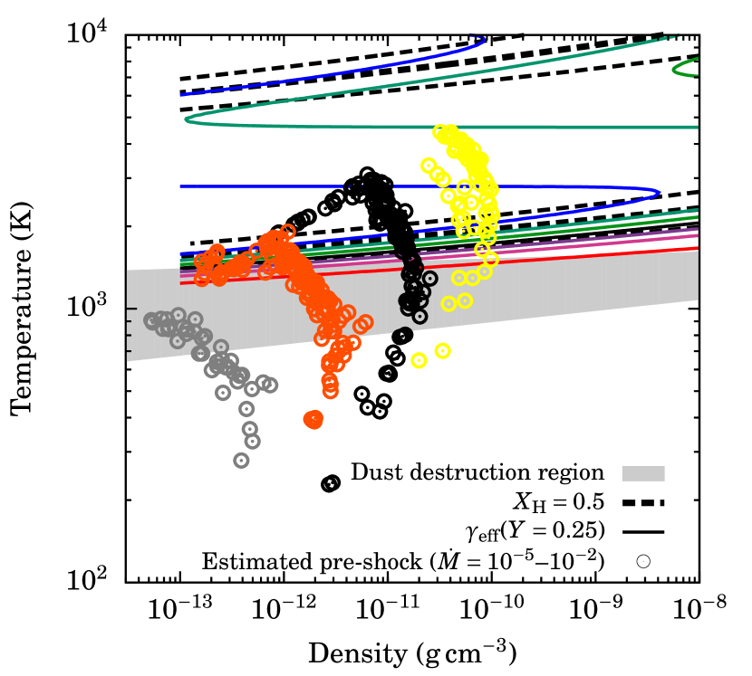
Figure 4: Estimate of the shock temperature and upstream density made by assuming $\eta^{\rm kin}=1$ (an isothermal shock), ${f_{\textnormal{red}}}=1$ upstream, and $L({r_{\rm shock}}^{-})\ll L({r_{\rm shock}}^{+})$, which leads to $4\pi{R_{\textnormal{p}}}^{2}caT_{\rm shock}^{4}\approx G{M_{\textnormal{p}}}{\dot{M}}/{R_{\textnormal{p}}}$ (see Equation (27)), with $\varrho$ given by the free-fall density (Equation (12)). Shown are contours of $\gamma=1.10$–1.40 in steps of 0.05 (blue through green to red) with $\gamma\approx 1.4$ from $\approx 100$ to 1000 K, as well as of the ionization or dissociation fraction for hydrogen of ${X_{\textnormal{H}}}=0.1$, 0.5, and 0.9 (black dashed lines), and the region of dust destruction in BL94 (grey band), with $\kappa$ of order 1 cm² g^-1 at lower $T$. The groups of points are, from left to right, for $\log{\dot{M}}/({M_{\oplus}}\,{\rm yr}^{-1})=-5$, $-4$, $-3$, and $-2$.

References

- Arras & Bildsten (2006) Arras, P., & Bildsten, L. 2006, ApJ, 650, 394
- Ayliffe & Bate (2009) Ayliffe, B. A., & Bate, M. R. 2009, MNRAS, 393, 49
- Baraffe et al. (2012) Baraffe, I., Vorobyov, E., & Chabrier, G. 2012, ApJ, 756, 118
- Bell & Lin (1994) Bell, K. R., & Lin, D. N. C. 1994, ApJ, 427, 987
- Berardo et al. (2016) Berardo, D., Cumming, A., & Marleau, G.-D. 2016, ArXiv e-prints, arXiv:1609.09126 [astro-ph.EP]
- Biller et al. (2013) Biller, B. A., Liu, M. C., Wahhaj, Z., et al. 2013, ApJ, 777, 160
- Bodenheimer et al. (2000) Bodenheimer, P., Hubickyj, O., & Lissauer, J. J. 2000, Icarus, 143, 2
- Bowler (2016) Bowler, B. P. 2016, ArXiv e-prints, arXiv:1605.02731 [astro-ph.EP]
- Brandt et al. (2014) Brandt, T. D., McElwain, M. W., Turner, E. L., et al. 2014, ApJ, 794, 159
- Chauvin et al. (2004) Chauvin, G., Lagrange, A.-M., Dumas, C., et al. 2004, A&A, 425, L29
- Clanton & Gaudi (2015) Clanton, C., & Gaudi, B. S. 2015, ArXiv e-prints, arXiv:1508.04434 [astro-ph.EP]
- Close et al. (2014) Close, L. M., Follette, K. B., Males, J. R., et al. 2014, ApJ, 781, L30
- Commerçon et al. (2011) Commerçon, B., Audit, E., Chabrier, G., & Chièze, J.-P. 2011, A&A, 530, A13
- D’Angelo & Bodenheimer (2013) D’Angelo, G., & Bodenheimer, P. 2013, ApJ, 778, 77
- D’Angelo et al. (2003) D’Angelo, G., Kley, W., & Henning, T. 2003, ApJ, 586, 540
- Drake (2006) Drake, R. P. 2006, High-Energy-Density Physics: Fundamentals, Inertial Fusion, and Experimental Astrophysics (Springer)
- Drake (2007) —. 2007, Physics of Plasmas, 14, 043301
- Ensman (1994) Ensman, L. 1994, ApJ, 424, 275
- Freedman et al. (2008) Freedman, R. S., Marley, M. S., & Lodders, K. 2008, ApJS, 174, 504
- Fung et al. (2015) Fung, J., Artymowicz, P., & Wu, Y. 2015, ArXiv e-prints, arXiv:1505.03152 [astro-ph.EP]
- Hartmann et al. (1997) Hartmann, L., Cassen, P., & Kenyon, S. J. 1997, ApJ, 475, 770
- Katarzyński et al. (2016) Katarzyński, K., Gawroński, M., & Goździewski, K. 2016, MNRAS
- Keith & Wardle (2015) Keith, S. L., & Wardle, M. 2015, MNRAS, 451, 1104
- Koenigl (1991) Koenigl, A. 1991, ApJ, 370, L39
- Kuiper et al. (2010) Kuiper, R., Klahr, H., Dullemond, C., Kley, W., & Henning, T. 2010, A&A, 511, A81
- Kuiper & Klessen (2013) Kuiper, R., & Klessen, R. S. 2013, A&A, 555, A7
- Lafrenière et al. (2008) Lafrenière, D., Jayawardhana, R., & van Kerkwijk, M. H. 2008, ApJ, 689, L153
- Lagrange et al. (2009) Lagrange, A.-M., Gratadour, D., Chauvin, G., et al. 2009, A&A, 493, L21
- LeBlanc & Wilson (1970) LeBlanc, J. M., & Wilson, J. R. 1970, ApJ, 161, 541
- Levermore (1984) Levermore, C. D. 1984, J. Quant. Spec. Radiat. Transf., 31, 149
- Levermore & Pomraning (1981) Levermore, C. D., & Pomraning, G. C. 1981, ApJ, 248, 321
- Lissauer et al. (2009) Lissauer, J. J., Hubickyj, O., D’Angelo, G., & Bodenheimer, P. 2009, Icarus, 199, 338
- Lovelace et al. (2011) Lovelace, R. V. E., Covey, K. R., & Lloyd, J. P. 2011, AJ, 141, 51
- Macintosh et al. (2014) Macintosh, B., Graham, J. R., Ingraham, P., et al. 2014, Proceedings of the National Academy of Science, 111, 12661
- Malygin et al. (2014) Malygin, M. G., Kuiper, R., Klahr, H., Dullemond, C. P., & Henning, T. 2014, A&A, 568, A91
- Marleau & Cumming (2014) Marleau, G.-D., & Cumming, A. 2014, MNRAS, 437, 1378
- Marley et al. (2007) Marley, M. S., Fortney, J. J., Hubickyj, O., Bodenheimer, P., & Lissauer, J. J. 2007, ApJ, 655, 541
- Marois et al. (2008) Marois, C., Macintosh, B., Barman, T., et al. 2008, Science, 322, 1348
- Mignone et al. (2007) Mignone, A., Bodo, G., Massaglia, S., et al. 2007, ApJS, 170, 228
- Mignone et al. (2012) Mignone, A., Zanni, C., Tzeferacos, P., et al. 2012, ApJS, 198, 7
- Mihalas & Mihalas (1984) Mihalas, D., & Mihalas, B. W. 1984, Foundations of radiation hydrodynamics (Oxford University Press)
- Mizuno (1980) Mizuno, H. 1980, Prog. Th. Phys., 64, 544
- Mordasini (2013) Mordasini, C. 2013, A&A, 558, A113
- Mordasini et al. (2012) Mordasini, C., Alibert, Y., Klahr, H., & Henning, T. 2012, A&A, 547, A111
- Oppenheimer et al. (2012) Oppenheimer, B. R., Beichman, C., Brenner, D., et al. 2012, in Society of Photo-Optical Instrumentation Engineers (SPIE) Conference Series, Vol. 8447, Society of Photo-Optical Instrumentation Engineers (SPIE) Conference Series, 20
- Ormel et al. (2015) Ormel, C. W., Shi, J.-M., & Kuiper, R. 2015, MNRAS, 447, 3512
- Paxton et al. (2013) Paxton, B., Cantiello, M., Arras, P., et al. 2013, ApJS, 208, 4
- Peters-Limbach et al. (2013) Peters-Limbach, M. A., Groff, T. D., Kasdin, N. J., et al. 2013, in Society of Photo-Optical Instrumentation Engineers (SPIE) Conference Series, Vol. 8864, Society of Photo-Optical Instrumentation Engineers (SPIE) Conference Series, 1
- Pollack et al. (1994) Pollack, J. B., Hollenbach, D., Beckwith, S., et al. 1994, ApJ, 421, 615
- Quanz et al. (2015) Quanz, S. P., Amara, A., Meyer, M. R., et al. 2015, ApJ, 807, 64
- Sallum et al. (2015) Sallum, S., Follette, K. B., Eisner, J. A., et al. 2015, Nature, 527, 342
- Semenov et al. (2003) Semenov, D., Henning, T., Helling, C., Ilgner, M., & Sedlmayr, E. 2003, A&A, 410, 611
- Skemer et al. (2014) Skemer, A. J., Hinz, P., Esposito, S., et al. 2014, in Society of Photo-Optical Instrumentation Engineers (SPIE) Conference Series, Vol. 9148, Society of Photo-Optical Instrumentation Engineers (SPIE) Conference Series, 12
- Spiegel & Burrows (2012) Spiegel, D. S., & Burrows, A. 2012, ApJ, 745, 174
- Stahler et al. (1980) Stahler, S. W., Shu, F. H., & Taam, R. E. 1980, ApJ, 241, 637
- Szulágyi et al. (2016) Szulágyi, J., Masset, F., Lega, E., et al. 2016, MNRAS, 460, 2853
- Tanigawa et al. (2012) Tanigawa, T., Ohtsuki, K., & Machida, M. N. 2012, ApJ, 747, 47
- Uribe et al. (2013) Uribe, A. L., Klahr, H., & Henning, T. 2013, ApJ, 769, 97
- Vaytet et al. (2013a) Vaytet, N., Chabrier, G., Audit, E., et al. 2013a, A&A, 557, A90
- Vaytet et al. (2013b) Vaytet, N., González, M., Audit, E., & Chabrier, G. 2013b, J. Quant. Spec. Radiat. Transf., 125, 105
- Zel’dovich & Raizer (1967) Zel’dovich, Y. B., & Raizer, Y. P. 1967, Physics of shock waves and high-temperature hydrodynamic phenomena (Academic Press)
- Zhu (2015) Zhu, Z. 2015, ApJ, 799, 16
- Zurlo et al. (2014) Zurlo, A., Vigan, A., Mesa, D., et al. 2014, A&A, 572, A85