LISA Detection of Binary Black Holes in the Milky Way Galaxy
Abstract
Using the black hole merger rate inferred from LIGO, we calculate the abundance of tightly bound binary black holes in the Milky Way galaxy. Binaries with a small semimajor axis () originate at larger separations through conventional formation mechanisms and evolve as a result of gravitational wave emission. We find that LISA could detect
them in the Milky Way. We also identify possible X-ray signatures of such binaries.
keywords:
Gravitational waves – (stars:) binaries: general – X-rays: binaries – stars: black holes1 Introduction
The Laser Interferometer Gravitation-Wave Observatory (LIGO) discovered gravitational waves from binary black holes (Abbott et al., 2016a, c), composed of black holes with masses .
Two stars in an isolated binary can evolve to produce the progenitors of the LIGO sources. To possess the observed parameters of the LIGO sources, these binaries must have progenitors with high masses () and low metallicities (Belczynski et al., 2016). The binary evolution could be initially affected by mass transfer through a common envelope phase.
However, in the chemically homogeneous evolution model (de Mink and Mandel, 2016; Mandel and de Mink, 2016), two massive stars in a near contact binary spin rapidly due to tidal spin-orbit coupling. The rapid rotation of a star mixes its interior, allowing transport of hydrogen from the envelope to the core and metals from the core to the envelope (Maeder, 1987). In contrast to the standard binary evolution model, the stars do not follow a common envelope phase, due to their contraction within their Roche lobes.
Regardless of the formation mechanism, none of the progenitor systems could directly produce two black holes at arbitrarily small separations. Here we focus on tight binary black holes with a semimajor axis smaller than could feasibly be created directly by conventional stellar evolution mechanisms. These binary black holes were born at a larger semimajor axis through standard evolution, and then migrated to smaller separations via gravitational wave emission. Most of these binary black holes reside in an intermediate regime, where their coalescence time is shorter than the Hubble time but longer than the LIGO operation lifetime before they become detectable in the LIGO frequency band.
We focus our analysis on binary black holes within the Milky Way galaxy. While most of our equations could be applied to binaries at arbitrary distances, the signatures of the systems under consideration are not observable outside of the Milky Way. We will assume circular orbits, as the detected LIGO binaries are constrained to possess low eccentricities (Abbott et al., 2016a). This means that we neglect binary black hole production via many body encounters and strong interactions in globular clusters (Sigurdsson and Hernquist, 1993; Rodriguez et al., 2015). Aside from these assumptions, we will remain agnostic as to the specific mechanism producing the binaries.
Recently, Seto (2016) used an estimate of the population of Galactic binary black holes to predict that LISA will have the sensitivities required to detect binaries like GW150914. In this article, we used a more sophisticated population analysis to show that the result can be generalized to more complicated population models. Furthermore, we extend the calculation to black hole populations with varying masses and take into account the black hole mass function.
In section 2 we perform a population analysis of tight binary black holes in the Milky Way. In section 3 we show that the gravitational wave signatures of these tight binaries are observable by LISA. In section 4 we examine possible X-ray signatures of these binaries. Finally, section 5 summarizes our conclusions.
2 Population analysis
The number of binary black holes at a given time with semimajor axis between and can be written as,
| (1) |
Assuming that their dynamical evolution is dominated by the emission of gravitational radiation, obeys a simple advection equation,
| (2) |
where and are the masses of the two black holes, is a source term that parameterizes the production of binaries at a semimajor axis , and is given by,
In the simple case of , the solution of equation (2) is given by
| (3) |
where is some arbitrary function. The simplest solution can be obtained in a steady state, where equation (2) reduces to
| (4) |
Integrating this equation gives
| (5) |
where is an arbitrary constant. This is a special case of the solution in equation (3), with .
The inferred merger rate from LIGO for two black holes is between and Gpc-3 yr-1 (Abbott et al., 2016b) in comoving units. We can estimate the Galactic merger rate by adopting the number of Milky Way-like galaxies to be per comoving Mpc3 (Montero-Dorta and Prada, 2009). Adopting Gpc-3 yr-1 as a fiducial LIGO inferred merger rate gives the LIGO Galactic merger rate to be mergers per galaxy per year.
A merger is detected by LIGO when the semimajor axis of the binary is small enough that it enters the LIGO frequency band. Denoting this critical semimajor axis as , the merger rate is equal to the flux in -space at ,
| (6) |
Therefore,
| (7) |
where we have substituted from equation (6). Using the inferred Galactic merger rate and specializing to binary black holes of mass , we can integrate over to obtain the number of Galactic binary black holes with semimajor axis ,
| (8) |
where is the solar radius and is the rate in units of .
2.1 Source functions with a minimum injection scale
Next, we generalize the population analysis to cases with a source function. Most formation mechanisms cannot produce binaries that are very tight. We model this situation with a source function that is proportional to a step function, , where is the minimum binary separation for the formation mechanism, is the Heavyside step function, and is an arbitrary function.
Given this source function, the general solution is,
| (9) |
as long as the function is not singular at . For example, a power law source with normalization and index , , admits the general solution,
| (10) |
Note also that in the case of a delta function source injected at , the solution is given by,
| (11) |
The most important feature of equation (9) is that the solution below the injection point, is unchanged from the sourceless case. This implies that as long as we restrict our analysis to , we can simply use the sourceless solution. Our results will therefore be robust due to its insensitivity to the particular binary black hole production mechanism.
2.2 Power-law source functions with a maximum injection scale
For the sake of generality, we also consider a source function without a minimum scale, namely with positive that extends all the way to . In principle, is related to the power law index of the binary separation of massive stars (Sana et al., 2012). However, as not all massive binaries evolve into binary black holes, the mapping between the two indices is unknown. Since binaries are not produced up to arbitrarily high semimajor axis, we truncate our source function at high values of by an exponential factor,
| (12) |
where , is some large semimajor axis above which binary black holes are rarely produced. This source function corresponds to a mechanism that produces binaries over a broad range of , where instead of a minimum injection scale, , we now have a maximum injection scale, . At large semimajor axes, this distribution corresponds to the end states of binary star evolution, whereas at small it corresponds to more exotic processes such as direct collapse (Loeb, 2016).
The binary population with this source term obeys
| (13) |
where and are constants that in principe can be constrained by observations. The general solution to this equation is given by,
| (14) |
where is an arbitrary function and is the incomplete Gamma function. As before, we can look for a steady state solution by setting the function to be a constant , giving
| (15) |
In this case, the merger rate equals the flux in -space at plus a term corresponding to the source,
| (16) |
where is the rate of binary black holes created with , given by,
| (17) |
Since , we get,
| (18) |
The number density of binary black holes is then given by,
| (19) |
where in the second equality we used the fact that both and are much smaller than unity. This result shows that in the case of a power law source function, the scaling of the sourceless solution remains valid even if the source function does not have a minimum scale as long as there is a maximum injection scale. The case of a power law with neither a maximum or minimum injection scale is treated in the Appendix.
2.3 Population analysis for varying black hole masses
In the previous sections, the abundance of binaries was derived for a given value of . In reality, the black hole population spans a range of masses with a probability given by the black hole mass function. Thus, the binaries possess varying values of . In this section we incorporate this diversity of values. Note that there is a single advection equation for every value of , i.e. there are many copies of equation (2), each for a different value of . To make explicit its dependence on , we label the density in equation (2) as . The total number of binary black holes per semimajor axis is given in terms of by,
| (20) |
where is the probability of finding a binary black hole with a particular value of . As is a function of the two black hole masses, its probability distribution is determined by the mass functions of the first and second black holes, and , respectively. For simplicity, we adopt , and the distribution can be obtained from by a series of convolutions. Adopting a phenomenological power-law relation, with an index and a normalization,
| (21) |
we can derive the normalization constant in terms of . Theoretically, the minimum value is obtained when both black holes are at the limit imposed by the Tolman-Oppenheimer-Volkoff equation of a Chandrasekhar-Landau mass () each. However, there is evidence that there exists a mass gap under (Ozel et al, 2010; Farr et al, 2011; Kreidberg et al., 2012). We thereby chose the minimum to be that when both black holes are each.
For our phenomenological model with , the integral converges and can be solved to give,
| (22) |
The merger rate is given by the sum over all masses of the fluxes in -space,
| (23) |
For the sourceless steady-state solution, , we can find in the phenomenological model by noting that,
| (24) |
For , this integral converges to
| (25) |
which implies that for ,
| (26) |
The number of binary black holes per unit semimajor axis is therefore given by,
| (27) |
The number of Galactic binary black holes with semimajor axis is given by
| (28) |
Aside from numerical factors of order unity the only change from the single case is that appears in the denominator in place of . Since is times smaller than the for two solar mass black holes, this number is of order larger than in equation (8).
2.4 Population analysis for varying black hole masses: Chabrier/Kroupa IMF
Next, we proceed beyond the phenomenological toy model for assuming that the black hole mass function follows the power-law dependence of massive stars, (Chabrier, 2003), where is a constant. We define the quantity,
| (29) |
so that the respective distribution follows,
| (30) |
If the masses and are independently distributed, can be derived from as follows. We first switch from the random variables and to and , where and,
| (31) |
where the positive root was chosen since , , and are positive definite. The distribution function is then given by,
| (32) |
where the determinant of the Jacobian of the transformation,
| (33) |
The marginal distribution is therefore,
| (34) |
which for the assumed mass function is given by,
| (35) |
Here, corresponds to the minimum and maximum black hole masses; in particular, is again chosen to be and , respectively.
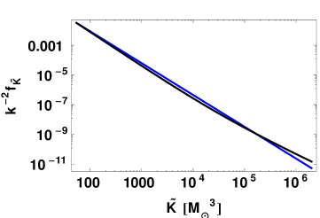
Although the integral in equation (35) could only be solved numerically, the distribution is well represented by a power law form between and with a negative index (see Figure 1). In order to simplify the analysis, we will therefore adopt,
| (36) |
where . This gives
| (37) | ||||
| (38) |
We proceed analogously to the previous section, where the main difference is that we now have an upper cutoff on black hole masses at .
For the steady state solution, , the rate of binary black holes entering the LIGO band is given by,
| (39) |
In equation (2.4), the integration limits refer to the maximum and minimum black hole masses that LIGO is sensitive to. The assumption that LIGO is sensitive to all black hole masses available in the black hole mass function translates to substituting and as these limits. Note that as the IMF is dominated by low mass black holes, our result is only weakly dependent on the exact value of . Using to eliminate the constant yields,
| (40) |
The abundance of binaries is therefore given by,
| (41) |
The number of binary black holes with semimajor axis is then,
| (42) | ||||
| (43) |
While this result is derived by assuming that the black hole mass function follows the power-law mass function of massive stars, simulations indicate that not all massive stars form black holes, and that stars above blow off too much of their mass to produce black holes (Sukhbold, 2016). These complications could lower the abundance of black holes relative to that predicted by equation (42). This means that our prediction should be interpreted as an upper bound to the number of binary black holes in the Galaxy.
2.5 Comparison with population synthesis models
In order to compare our result to population synthesis models, we first transform our variable from to the frequency . The number of binary black holes with semimajor axis is equal to the number of binary black holes with frequency , where is the orbital period of the smallest black holes in the population with separation .
For the systems under consideration, and the smallest black hole mass is , resulting in a minimum frequency of Hz. Equation (42) therefore predicts binary black holes in the Galaxy with frequency greater than Hz.
The population synthesis model A of Belczynski et al. (2010) predicts thousands of binary black holes with frequencies greater than Hz. Noting that the LIGO rate ranges from to , this is consistent with our result. An earlier calculation by Nelemans et al. (2001) predicts a number that is an order of magnitude larger than model A of Belczynski et al. (2010), which is still consistent with our result.
3 Gravitational wave signal from Milky Way binaries
Most of the Galactic binary black holes with orbital separation , will not enter the LIGO bandpass in a short enough time for them to be observed by LIGO. For example, the timescale for two black holes to coalesce from a few is thousands of years. These binaries, however, will be observable by LISA111http://www.elisascience.org which is sensitive to lower frequencies than LIGO.
Focusing on the case of two black holes, we find from equation (8) that the tightest binary black hole in our Galaxy has . For such a binary consisting of two black holes, the gravitational wave frequency is Hz, which is within the LISA bandpass (Farmer and Phinney, 2003). The angular-averaged gravitational wave strain for the mode is given by (Peters and Mathews, 1963; Seto, 2016),
| (44) |
where is the chirp mass. Integrating the signal over an observational period , the signal to noise ratio becomes (Seto, 2016),
| (45) |
where is the LISA instrumental noise, with a value of at mHz (Amaro-Seoane et al., 2012). Scaling the noise with frequency as the power law (Seto, 2016), the signal to noise ratio becomes,
| (46) |
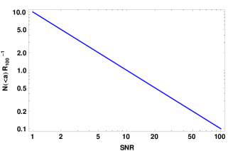
For observations across the Milky Way with kpc, we find,
| (47) |
Figure 2 shows the expected number of such Milky Way binaries as a function of their SNR.
3.1 Confusion with cosmological sources
A supermassive binary black hole at cosmological distances can possess similar values of strain amplitude and frequency to a Galactic binary black hole, thus masquerading as a Galactic source. However, this confusion can be eliminated by measuring the change in gravitational wave frequency as a function of time, .
The time derivative of the gravitational wave frequency is given by (Cutler and Flanagan, 1994)
| (48) |
Supermassive binary black holes possess chirp masses that are much greater than that of Galactic binaries. As such, their frequency changes at a much faster pace than Galactic binaries.
4 Electromagnetic flag
4.1 Binary black hole accretion in a hierarchical triple system
A binary black hole could accrete gas if it resides in a hierarchical triple system, where the third object is a main sequence star. The wind of the third star would lead to accretion at the Bondi-Hoyle-Lyttleton rate (Hoyle and Lyttleton, 1939; Bondi and Hoyle, 1944),
| (49) |
where , the mass density of the stellar wind, the wind speed, and is the sound speed, with be the wind temperature. Scaling the wind parameters to solar values at a distance of AU and assuming an efficiency of for converting rest mass into radiation, the luminosity produced by the binary where both black holes are solar masses is,
| (50) |
where is the separation of the star from the binary. The maximum luminosity is given by the Eddington limit,
| (51) |
Due to the orbital motion of the black holes around the center of mass, the observed flux would be modulated by Doppler beaming. Assuming that the emitted flux, scales with frequency as , the Doppler modulation is given by
| (52) |
where is the observed flux, and is the Doppler factor. To first order, the flux modulation is given by (D’Orazio, Haiman, and Schiminovich, 2015),
| (53) |
where is the orbital phase and the inclination.
At the Eddington luminosity, the amplitude of the flux modulation of two binary, is given by,
| (54) |
where is the distance to the object and we have assumed (Sobolewska et al., 2011; D’Orazio, Haiman, and Schiminovich, 2015). Given the flux sensitivity of XRM-Newton of , for a semimajor axis of , the flux modulation of these objects will be observable out to Mpc.
Realistically, it is unlikely for such binaries to emit at the Eddington luminosity. For general Bondi-Hoyle-Lyttleton accretion, the flux modulation depends on the binary and stellar wind parameters,
| (55) |
Substituting the solar wind parameters at AU and the XRM-Newton sensitivity for yields for the observer distance of pc at which a pair of black holes will be detectable. The X-ray surveyor222http://wwwastro.msfc.nasa.gov/xrs/, a next generation x-ray observatory with a flux sensitivity of , will be able to detect this flux modulation out to a distance of kpc, which allows their detection throughout the entirety of the Milky Way galaxy.
Owing to the fact that most massive stars are in multiple systems (Raghavan et al., 2010; Tokovinin, 2014), and that there is precedent for X-ray binaries in triple systems (Grindlay et al, 1988; Thorsett et al, 1999; Chou and Grindlay, 2001; Zdziarski et al., 2007; Prodan and Murray, 2015), most binary black holes will likely possess a third companion. Further evidence of this comes from observations of superorbital modulations in high-mass X-ray binary systems, which could be caused by a third companion (Farrell, Sood, and O’Neill, 2006; Corbet and Krimm, 2013). However, only a fraction of binary black holes in a hierarchical triplet would host companions in the relevant mass range for accretion to be efficient. Since only companions with masses and above generates sufficient luminosity to be observed throughout the Milky Way, the percentage of observable systems is
| (56) |
where is the stellar IMF, yr is the Hubble time, and is the main sequence lifetime of the companion star, given by the broken power law (Laughlin, Bodenheimer and Adams, 1997; Salaris and Cassisi, 2006; Loeb, Batista, and Sloan, 2016)
| (57) |
where for stars less massive than and for more massive stars. The ratio in equation (56) takes into account both the stellar IMF and the fact that more massive stars live a shorter amount of time. Substituting the Chabrier IMF for , we obtain,
| (58) |
This implies that out of the black holes with predicted by equation (8), only a few systems would host the appropriate companion to be observable throughout the entirety of the Milky Way. This number is further diminished by the fact that only a fraction of all triple systems have the stars at a close enough distance, as the signal scales as . We therefore conclude that the most efficient method to detect these binaries is through their gravitational wave emission with LISA.
4.2 Tidal disruption flares from planets and asteroids
Another source of electromagnetic activity could be associated with the tidal disruption of planets and asteroids by the black holes. White dwarfs and neutron stars are known to host rocky debris around them (Vanderburg et al., 2015; Zuckerman et al., 2010; Farihi et al, 2009; Koester et al., 2014; Wolszczan and Frail, 1992; Podsiadlowski, 1993; Phinney and Hansen, 1993). Orbits around binary black holes can be chaotic and are subject to Kozai-Lidov oscillations, leading to an enhanced tidal disruption rate (Ivanov et al., 2005; Chen et al., 2009; Li et al., 2015).
For a planet or asteroid of mass and radius being tidally disrupted by a black hole of mass , the length of the flare is defined as the time it takes for the emission to drop under the Eddington limit. This is given by (Ulmer, 1998),
| (59) |
where the pericenter distance and the tidal radius. Assuming a Neptune-like planet with g and cm, the flare time becomes years.
Since this timescale is much longer than the orbital timescale, lightcurves from these events will possess amplitude modulation due to the Doppler effect, as described in section 4.1. The Doppler modulation of such systems is bright enough to be detectable from throughout the Milky Way by existing telescopes such as the XMM-Newton and the Chandra X-ray Observatory. As the number of sources in the sky per unit time will depend on the duty cycle of such flares, a monitoring campaign of a large patch of the sky is required to find such flaring sources. Confusion with other sources would make the identification of such binaries difficult.
5 Conclusions
By calibrating the population of binary black holes based on the merger rate infered by LIGO, we have found that LISA could detect a handful of such binaries in the Milky Way galaxy (see Figure 2). A lack of detections will set constraints on the binary production mechanisms.
We also considered electromagnetic flags of these tight binary black holes in the Milky way, and found them to have weaker observational prospects. Gravitational wave signals could be leveraged to provide both the system’s masses and semimajor axis.
6 Acknowledgements
The authors thank Josh Grindlay for comments on the manuscript. This work was supported in part by the Black Hole Initiative at Harvard University, funded by the John Templeton Foundation.
References
- Abadie et al. (2010) Abadie et al., The LIGO Scientific Collaboration and the Virgo Collaboration, 2010, Classical and Quantum Gravity, 27, 17, 173001
- Abbott et al. (2016a) Abbot et al., The LIGO Scientific Collaboration and the Virgo Collaboration, 2016, Physical Review Letters, 116, 6, 061102
- Abbott et al. (2016b) Abbot et al., The LIGO Scientific Collaboration and the Virgo Collaboration, 2016, arXiv:1602.03842
- Abbott et al. (2016c) Abbot et al., The LIGO Scientific Collaboration and the Virgo Collaboration, 2016, Physical Review Letters, 116, 241103
- Amaro-Seoane et al. (2012) Amaro-Seoane P., et al., 2012, Classical Quantum Gravity, 29, 124016
- Belczynski et al. (2016) Belczynski, K. and Holz, D.E. and Bulik, T. and O’Shaughnessy, R., 2016, Nature, 534, 512-515
- Belczynski et al. (2010) Belczynski, K., Benacquista, E., and Bulik, T., 2010, ApJ, 725, 816-823
- Bondi and Hoyle (1944) Bondi, H. and Hoyle, F. 1944, MNRAS, 104, 273
- Chabrier (2003) Chabrier, G., 2003, Publications of the Astronomical Society of the Pacific, 115, 763-795
- Chen et al. (2009) Chen, X., Madau, P., Sesana, A., and Liu, F. K., Astrophysical Journal, 697, L149-L152
- Chou and Grindlay (2001) Chou, Y and Grindlay, J. E., ApJ, 563, 934-940
- Corbet and Krimm (2013) Corbet, Robin H. D.; Krimm, Hans A., 2013, ApJ, 778, 45C
- Cutler and Flanagan (1994) Curt Cutler and anna E. Flanagan, 1994, Phys. Rev. D 49, 2658
- de Mink and Mandel (2016) de Mink, S.E. and Mandel, I., 2016, MNRAS, 460, 3545-3553
- D’Orazio, Haiman, and Schiminovich (2015) D’Orazio, D. J.; Haiman, Z.; Schiminovich, D., 2015, Nature, 525, 351-353
- Farmer and Phinney (2003) Farmer, A. J. and Phinney, E. S., 2003, MNRAS, 346, 1197-1214
- Farr et al (2011) Farr, W. M., Sravan, N., Cantrell, A., et al. 2011, ApJ, 741, 103
- Farrell, Sood, and O’Neill (2006) Farrell, S. A.; Sood, R. K.; O’Neill, P. M., 2006, MNRAS,367,1457
- Farihi et al (2009) Farihi, J., Jura, M. & Zuckerman, B., 2009, Astrophys. J. 694, 805-819.
- Grindlay et al (1988) Grindlay, J. E.; Bailyn, C. D.; Cohn, H.; Lugger, P. M.; Thorstensen, J. R.; Wegner, G., ApJ, 334, L25-L29
- Hoyle and Lyttleton (1939) Hoyle, F. and Lyttleton, R. A., 1939, Proceedings of the Cambridge Philosophical Society, 35, 405
- Ivanov et al. (2005) Ivanov P.B., Polnarev, A. G. and Saha P., 2005, MNRAS, 358, 1361
- Koester et al. (2014) Koester, D., G nsicke, B. T. & Farihi, J., 2014, Astron. & Astrophys. 566, A34 (2014).
- Kreidberg et al. (2012) Kreidberg, L., Bailyn, C. D., Farr, W. M., & Kalogera, V. 2012, ApJ, 757, 36
- Li et al. (2015) Gongjie, Li., Naoz, S., Kocsis, B., and Loeb, A., MNRAS, 451, 1341-1349
- Laughlin, Bodenheimer and Adams (1997) G. Laughlin, P. Bodenheimer and F. C. Adams, 1997, The Astrophysical Journal, 482, 420-432
- Montero-Dorta and Prada (2009) Montero-Dorta, A.D., and Prada, F., 2009, MNRAS, 399, 1106
- Loeb, Batista, and Sloan (2016) Loeb, A., Batista, R.A., and Sloan D., 2016, JCAP, 8, 40
- Loeb (2016) Loeb, A., 2016, ApJ, 819, L21
- Maeder (1987) Maeder, A., 1987, Astronomy and Astrophysics, 178, 159
- Mandel and de Mink (2016) Mandel, I. and de Mink, S.E., 2016, MNRAS, 458, 2634-2647
- Maeder (1987) Maeder, A., 1987, Astronomy and Astrophysics, 178, 159
- Nelemans et al. (2001) Nelemans, G., Yungelson, L. R, and Portegeis Zwart, S. F., 2001, Astronomy and Astrophysics, 375, 890-898
- Ozel et al (2010) Ozel, F., Psaltis, D., Narayan, R., & McClintock, J. E. 2010, ApJ, 725, 1918
- Peters and Mathews (1963) Peters P.C. and Mathews J., 1963, Phys. Rev., 131, 435
- Phinney and Hansen (1993) Phinney, E. S., and Hansen, B.M.S., 1993, ASP Conf. Ser., 36, 371
- Podsiadlowski (1993) Podsiadlowski, P., 1993, ASP Conf. Ser., 36, 149
- Prodan and Murray (2015) Prodan, Snezana; Murray, Norman, 2015, ApJ, 798, 117
- Salaris and Cassisi (2006) M. Salaris and S. Cassisi, 2006, Evolution of Stars and Stellar Populations
- Sana et al. (2012) Sana, H., de Mink, S. E., de Koter, A., Langer, N., Evans, C.J., et al., 2012, Science, 337, 444
- Seto (2016) Seto, N., 2016, MNRAS, 460, L1-L4
- Sigurdsson and Hernquist (1993) Sigurdsson, S., and Hernquist, L. ,1993, Nature, 364, 423
- Sobolewska et al. (2011) Sobolewska, M.A., Siemiginowska, A., Gierlinski, M., 2011, MNRAS, 413, 2259-2268
- Sukhbold (2016) Sukhbold, T., Ertl, T., Woolsley, S. E., Brown, J. M., and Janka, H. T., 2016, ApJ, 821, 38
- Raghavan et al. (2010) Raghavan, D., McAlister, H. A., Henry, T. J., Latham, D. W., Marcy, G. W.,Mason, B. D., Gies, D. R., White, R. J., and ten Brummelaar, T. A. 2010,ApJS, 190, 1
- Rodriguez et al. (2015) Rodriguez, C. L., Morscher, M., Pattabiraman, B., Chatterjee, S., Haster, C.-J., and Rasio, F. A. 2015, Physical Review Letters, 115, 051101
- Thorsett et al (1999) Thorsett, S. E.; Arzoumanian, Z.; Camilo, F.; Lyne, A. G., ApJ, 523, 763-770
- Tokovinin (2014) Tokovinin, A. 2014, AJ, 147, 87
- Ulmer (1998) Ulmer, A., 1998, American Institute of Physics Conference Series, 431, 141-144
- Vanderburg et al. (2015) Vanderburg, A., Johnson, J.A., Rappaport, S., Bieryla, A., Irwin, J., et al., 2015, Nature, 526, 546-549
- Wolszczan and Frail (1992) Wolszczan, A. and Frail, D., 1992, Nature, 355, 145
- Zdziarski et al. (2007) Zdziarski, Andrzej A.; Wen, Linqing; Gierli?ski, Marek, 2007, MNRAS. J. 377, 1006-1016
- Zuckerman et al. (2010) Zuckerman, B., Melis, C., Klein, B., Koester, D. & Jura, M., 2010 Astrophys. J. 722, 725 736
7 Appendix
7.1 Power law source functions without a minimum or maximum scale
Consider a nonzero, time-independent power-law source term that extends all the way from to . Unlike the example considered in the main text, we consider a case without a smallest injection scale or an upper cutoff scale. The binary black hole population with this source term obeys
| (60) |
where and are constants that in principe can be either derived or estimated from observations. The general solution to this equation is given by
| (61) |
where is an arbitrary function. As before, we search for a steady state solution by setting the function to be the constant , giving
| (62) |
In this case, the merger rate is equal to the flux in -space at plus a term corresponding to the source term,
| (63) |
where is the rate of binary black holes created per year with semimajor axis , given by
| (64) |
In this case,
| (65) |
which allows us to deduce that . Therefore, the number of Galactic binary black holes with semimajor axis is given by
| (66) | ||||
| (67) |
where is the number of Galactic binary black holes in the source-less case. Note that when we set the source term to zero by using , we will recover the sourceless solution. The effect of such a source term with , i.e. where there is a higher rate of binary black hole production at large semimajor axis, is paradoxically a suppression of the number of binary black holes in the steady state solution due to the requirement that the rate be kept unchanged. Since a source function that does not have a maximum injection scale is unphysical, the solution we obtain is also unphysical. In this case, there is a scale, , above which becomes negative. This calculation should be viewed only as a pedagogical toy model to illustrate an example of the ramifications of modifying one of our assumptions.
7.2 Population analysis for varying black hole masses: Power law source
We can repeat the analysis for the case of a power law source term. In this case we have,
| (68) |
where, inspired by our previous solutions, we have explicitly written out the dependency of so that it is now a constant with respect to . The merger rate is therefore given by,
| (69) |
which converges when to
| (70) |
Here is again the rate of binary black holes created per year with semimajor axis . However, in order to be consistent with our choice of the black hole mass function, we need to take into account the fact that different amounts of binary black holes are created for different black hole masses. Equivalently, binary black holes with different ’s are produced at different abundances. As a result, has to include an extra integral over ,
| (71) |
When , this integral converges to,
| (72) |
Following through, this gives the number of binary black holes per unit semimajor axis to be,
| (73) |
when . Note that when we set the source term to zero through , we will recover the sourceless solution. The number of binary black holes per unit semimajor axis is therefore,
| (74) |
where is the solution in the sourceless case and the number of binary black holes with semimajor axis is given by,
| (75) |
where as before is the sourceless solution. This solution is again pathological due to the presence of a critical semimajor axis above which becomes negative.