A Novel Quantum Image Compression Method Based on JPEG

Abstract

Quantum image processing has been a hot topic. The first step of it is to store an image into qubits, which is called quantum image preparation. Different quantum image representations may have different preparation methods. In this paper, we use GQIR (the generalized quantum image representation) to represent an image, and try to decrease the operations used in preparation, which is also known as quantum image compression. Our compression scheme is based on JPEG (named from its inventor: the Joint Photographic Experts Group) — the most widely used method for still image compression in classical computers. We input the quantized JPEG coefficients into qubits and then convert them into pixel values. Theoretical analysis and experimental results show that the compression ratio of our scheme is obviously higher than that of the previous compression method.

1 Introduction

Recently, quantum image processing has attracted a lot of attention. In general, it has three steps as Fig. 1 shows: 1) store the image into a quantum system, which is also known as preparation; 2) process the quantum image; and 3) obtain the result by measurement. In this paper, we will focus on quantum image preparation and focus on increasing preparation efficiency.

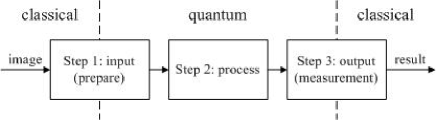
Figure 1: The processing steps of quantum image processing.

Quantum preparation is related to how an image is stored in a quantum system, which is known as quantum representation. Different quantum image representations may have different preparation methods. Researchers have proposed a number of quantum image representation schemes, such as Qubit Lattice [1], Real Ket [2], Entangled Image [3], FRQI (the flexible representation of quantum images) [4], MCQI (the RGB multi-channel representation for quantum images) [5], NEQR (the novel enhanced quantum representation of digital images) [6], QUALPI (the quantum representation for log-polar images) [7], QSMC$\&$QSNC (quantum states for $M$ colors and quantum states for $N$ coordinates) [8], NAQSS (the normal arbitrary quantum superposition state) [9], INEQR (the improved NEQR) [10], GQIR (the generalized quantum image representation)[11], and etc. A number of papers have summarized and compared them [11-12].

In this paper, we discuss GQIR’s compression. GQIR is developed from FRQI. FRQI, NEQR, INEQR and GQIR belong to one class. They are approbated and used more commonly. Their feature is that they use two entangled state sequences to represent color information and location information respectively. Fig. 2 gives the development and the inheritance of this class of representation.

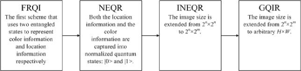
Figure 2: The development and the inheritance of the main class of quantum image representation.

GQIR uses $h=\lceil\log_{2}H\rceil$ qubits for $Y$-coordinate and $w=\lceil\log_{2}W\rceil$ qubits for $X$-coordinate to represent a $H\times W$ image. Both the location information and the color information are captured into normalized quantum states: $|0\rangle$ and $|1\rangle$. Hence, an GQIR image can be written as

$$|I\rangle=\frac{1}{\sqrt{2}^{h+w}}\left(\sum_{Y=0}^{H-1}\sum_{X=0}^{W-1}|C_{YX}\rangle|YX\rangle\right)$$ (1)

$$|YX\rangle=|Y\rangle|X\rangle=|y_{h-1}y_{h-2}\ldots y_{0}\rangle|x_{w-1}x_{w-2}\ldots x_{0}\rangle,\ y_{i},x_{i}\in\{0,1\}$$

$$|C_{YX}\rangle=|C^{q-1}_{YX}C^{q-2}_{YX}\ldots C^{0}_{YX}\rangle,C^{i}_{YX}\in\{0,1\}$$

where, $q$ is the color depth, and

$$h=\left\{\begin{array}[]{ll}\lceil\log_{2}H\rceil,&H>1\\ 1,&H=1\end{array}\right.$$

$$w=\left\{\begin{array}[]{ll}\lceil\log_{2}W\rceil,&W>1\\ 1,&W=1\end{array}\right.$$

$|YX\rangle$ is the location information and $|C_{YX}\rangle$ is the color information. It needs $h+w+q$ qubits to represent a $H\times W$ image with gray range $2^{q}$. Note that GQIR can represent not only gray scale images but also color images because the color depth $q$ is a variable. In most cases, when $q=2$, it is a binary image; when $q=8$, it is a gray scale image; and when $q=24$, it is a color image.

We choose GQIR procedure because:

1. It fully exploits the physical properties of qubits (entanglement and superposition) and reduces the number of qubits used to store an image.

2. It resolves the real-time computation problem of image processing and provides a flexible method to process any part of a quantum image by using controlled quantum logic gates.

3. It can represent a quantum image with any size.

4. It is close to the classical image representation. Hence, it is easier for researchers to understand and to transplant classical image processing algorithm into quantum system.

There are also some researchers believe that measurement is a fatal shortcoming of GQIR because measuring the quantum image one time, only one pixel is retrieved and the qubits collapse to the pixel, i.e., other pixels are disappeared. If a user want to retrieve the whole image, one must prepare, process and measure the image many, many times. However, we believe this is due to the wrong use, rather than GQIR itself. It is suitable to solve the problems with small amount output and can not be solved efficiently in classical computers. In Ref. [13-14], we have given a more detailed exposition and two example algorithms about this issue.

Quantum image compression is the procedure that reduces the quantum resources used to prepare quantum images [4]. The main resource in quantum preparation is the number of quantum gates instead of the number of qubits, because as stated previously, the number of qubits used in quantum images (i.e., $h+w+q$) has been very fewer than the number of bits used in classical images (i.e., $HWq$). Furthermore, the number of quantum gates can be used to indicate the network time complexity because in quantum network, each quantum gate is an operation which needs a certain amount of time to do it. Hence, in this paper, we only study network time complexity and simply refer to as network complexity, or complexity in the following. Therefore, the main task of quantum image compression is to reduce the number of gates used during quantum image preparation.

In Ref. [4] and [6], the minimization of Boolean expressions is used to compress the image preparation. We call it Boolean expression compression (BEC) method and will introduce it in detail in Section 2.1. However, BEC has some defects that prompt us to give a new compression scheme: 1) it needs a time-consuming preprocessing; and 2) the compression ratio is unstable.

Hence, this paper gives a new compression scheme. The new one is based on JPEG which is the most widely used method for still image compression in classical computers. We call the new one as quantum image JPEG compression, or the JPEG scheme. It inputs the quantized JPEG coefficients into qubits and then convert them into pixel values. Since the data amount of the JPEG coefficients are significantly less than that of the pixel values, the JPEG scheme can compress an image. Theoretical analysis and experimental results show that the compression ratio of our scheme is obviously higher than that of BEC.

The rest of the paper is organized as follows. Sect. 2 presents related works about BEC, JPEG and two quantum modules used in our scheme. Our scheme is discussed in Sect. 3 including the basic ideas and the scheme steps. Sect. 4 gives the theoretical analysis and experimental results. Sect. 5 gives the conclusion.

2 Related works

2.1 GQIR preparation and compression

A GQIR’s preparation is composed of $h+w$ Hadamard gates and some ($h+w$)-CNOT gates (CNOT gates with ($h+w$) control qubits). $h+w$ Hadamard gates are used to let state $|0\rangle$ and state $|1\rangle$ appear with equal probability in $|YX\rangle$, and ($h+w$)-CNOT gates are used to set the color information and entangle the color information and location information.

In Fig. 3 (a)-(c), an image with 4 pixels is given as an example to explain GQIR representation and preparation. In (a), one square indicates one pixel and the number in each square is the decimal pixel value. In (b), the number in $|\ \rangle$ before each $\otimes$ is the binary pixel value and the number in $|\ \rangle$ after each $\otimes$ is the binary location information. There are 4 such formulas superposed because the image has 4 pixels. In (c), 2 Hadamard gates generate the 4 location information $|00\rangle,|01\rangle,|10\rangle,|11\rangle$ and 10 2-CNOT gates are used to set the color information. Since all of the color qubits’ initial state is $|0\rangle$, the number of CNOT gates is equal to the number of “1” in the color information.

BEC method has been used to compress GQIR, which is based on the minimization of Boolean expressions. If $x$ is a Boolean variable and the value of it is 1 then the lateral $x$ is used in the minterm, otherwise the lateral $\overline{x}$ is used. Then, for example, a Boolean expression

$$e=x_{2}\overline{x_{1}}x_{0}+x_{2}x_{1}x_{0}$$

is minimized as

$$e=x_{2}x_{0}.$$

That is to say, if two CNOT gates operate the same color qubit and only one of their control qubits is different, the two CNOT gates can be combined into one gate. For example, in Fig. 3(b), the subspace

$$\begin{split}|C^{7}y_{0}x_{0}\rangle&=\frac{1}{2}(|0\rangle\otimes|00\rangle+|1\rangle\otimes|01\rangle+|1\rangle\otimes|10\rangle+|1\rangle\otimes|11\rangle)\\ &=\frac{1}{2}(|0\rangle\otimes|00\rangle+|1\rangle\otimes|01\rangle+|1\rangle\otimes|1\rangle(|0\rangle+|1\rangle))\end{split}$$

In the first line, $C^{7}$ has three $|1\rangle$, i.e., three CNOT gates are needed; in the second line, because the last two items are combined, $C^{7}$ has two $|1\rangle$ and only two CNOT gates are needed. Fig. 3(d) compresses the whole example image. It can be seen that BEC drops the number of CNOT gates from 10 to 6.

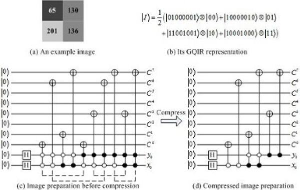
Figure 3: GQIR representation, preparation and compression.

However, the BEC method has some defects:

1. In fact, BEC has two steps: 1) preprocess: determining which CNOT gates can be combined; and 2) input: using Hadamard gates and CNOT gates to input the image into quantum system. The time complexity of BEC is

   $$C_{\text{BEC}}=C_{\text{p}}+C_{\text{i}}$$ (2)

   where $C_{\text{p}}$ is the complexity of preprocessing and $C_{\text{i}}$ is the complexity of inputting. The preprocessing is time consuming because we have to look over all the CNOT gates $C_{YX}^{i}$ before compression one pair by one pair. The looking over algorithm is shown below.

   Algorithm 1 The looking over algorithm

   1:  for all $i=0$ to $(q-1)$ do

   2:     for all $Y_{1}X_{1}=0$ to $(2^{2n}-1)$ do

   3:        for all $Y_{2}X_{2}=Y_{1}X_{1}+1$ to $(2^{2n}-1)$ do

   4:           if $C_{Y_{1}X_{1}}^{i}=C_{Y_{2}X_{2}}^{i}=1$ and only one bit of the binary $Y_{1}X_{1}$ and the binary $Y_{2}X_{2}$ is different then

   5:              Combine the two CNOT gate $C_{Y_{1}X_{1}}^{i}=1$ and $C_{Y_{2}X_{2}}^{i}=1$ to one;

   6:           end if;

   7:        end for;

   8:     end for;

   9:  end for;

   Hence, the complexity of the looking over algorithm is $O(q\cdot 2^{4n})$.

   Moreover, looking over one round is not enough because two combined gates may be combined further. Combining two CNOT gate one time, the number of control qubits will reduce one. Hence, the looking over process should be executed $2n$ round. Therefore, to a $2^{n}\times 2^{n}$ image, the complexity of preprocessing is

   $$C_{\text{p}}=O(2n\cdot q\cdot 2^{4n}).$$ (3)

   It is a very high complexity, and in most application scenarios, it is intolerable. Moreover, it is even much higher than the complexity before compression: $O(q2^{2n})$. Hence, even assuming that $C_{\text{i}}$ is 0, BEC method increases the complexity instead of playing the role of compression.

2. The compression ratio of this method is influenced by the bit planes. It is difficult to give an equation to calculate the compression ratio. Sometimes, the compression ratio is high (for an extreme example, all the pixels have the same color); and sometimes, maybe, no one CNOT gate can be compressed. That is to say, $C_{\text{i}}$ has no exact value.

For more information about GQIR, please refer Ref. [11].

2.2 JPEG compression [15-16]

JPEG is a commonly used method of lossy compression for digital still images. The degree of compression can be adjusted, allowing a selectable tradeoff between storage size and image quality. The typically compression ratio is 10:1 with little perceptible loss in image quality. The term “JPEG” is an acronym for the Joint Photographic Experts Group, which created the standard.

2.2.1 JPEG compression

The JPEG encoding process consists of the following steps (taking a gray scale image as an example):

1. Discrete cosine transform

   The image is split into blocks of $8\times 8$ pixels, and each block (denoted as $f(i,j)$, $i=0,1,\cdots,7$, $j=0,1,\cdots,7$) undergoes the discrete cosine transform (DCT) to get frequency spectrum $F(u,v)$.

   $$F(u,v)=c(u)c(v)\sum_{i=0}^{7}\sum_{j=0}^{7}\left\{f(i,j)\cos\left[\frac{(i+0.5)\pi}{8}u\right]\cos\left[\frac{(j+0.5)\pi}{8}v\right]\right\}$$ (4)

   where $u=0,1,\cdots,7$, $v=0,1,\cdots,7$, and

   $$c(u)=\left\{\begin{array}[]{c}\frac{1}{2\sqrt{2}},u=0\\ \frac{1}{2},u\neq 0\\ \end{array}\right.$$

   $F(0,0)$ is the direct-current coefficient, and the bigger $u$ and $v$, the higher frequency components $F(u,v)$.

2. Quantization

   The human eye is good at seeing small differences in brightness over a relatively large area, but not so good at distinguishing the exact strength of a high frequency brightness variation. This allows one to greatly reduce the amount of information in the high frequency components. This is done by simply dividing each component in the frequency domain by a constant for that component, and then rounding to the nearest integer. This rounding operation is the only lossy operation in the whole process if the DCT computation is performed with sufficiently high precision. As a result of this, it is typically the case that many of the higher frequency components are rounded to zero, and many of the rest become small positive or negative numbers, which take many fewer bits to represent. The elements in the quantization matrix control the compression ratio, with larger values producing greater compression. A typical quantization matrix is as follows:

   $$Q=\left[\begin{array}[]{ccccccccccccccc}16&&11&&10&&16&&24&&40&&51&&61\\ 12&&12&&14&&19&&26&&58&&60&&55\\ 14&&13&&16&&24&&40&&57&&69&&56\\ 14&&17&&22&&29&&51&&87&&80&&62\\ 18&&22&&37&&56&&68&&109&&103&&77\\ 24&&35&&55&&64&&81&&104&&113&&92\\ 49&&64&&78&&87&&103&&121&&120&&101\\ 72&&92&&95&&98&&112&&100&&103&&99\\ \end{array}\right]$$ (5)

   The quantized DCT coefficients are computed with

   $$F_{Q}(u,v)=round\left(\frac{F(u,v)}{Q(u,v)}\right)$$ (6)

3. Zigzag

   Because so many coefficients in the DCT image are truncated to zero values during the coefficient quantization stage, the zeros are handled differently than non-zero coefficients. They are coded using a Run-Length Encoding (RLE) algorithm. RLE gives a count of consecutive zero values in the image, and the longer the runs of zeros, the greater the compression. One way to increase the length of runs is to reorder the coefficients in the zigzag sequence shown in Fig. 4. This way, coefficients 0 are omitted and a terminator “EOF” is used.

   

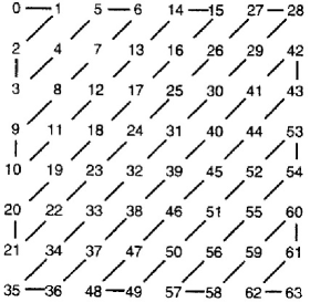
   Figure 4: Zigzag.

2.2.2 JPEG decompression

If we want to resume the pixel values, for example if we want to display the image on the screen, the inverse process is executed:

1. Rearrange the compressed data to $8\times 8$ blocks.

2. Multiply each $8\times 8$ block with the quantization matrix $Q$.

   $$F^{\prime}(u,v)=F_{Q}(u,v)\times Q(u,v)$$ (7)

3. Do inverse DCT (IDCT) to each $8\times 8$ block to get the recovered pixel value $f^{\prime}(i,j)$:

   $$f^{\prime}(i,j)=\sum_{u=0}^{7}\sum_{v=0}^{7}\left\{c(u)c(v)F^{\prime}(u,v)\cos\left[\frac{(i+0.5)\pi}{8}u\right]\cos\left[\frac{(j+0.5)\pi}{8}v\right]\right\}$$ (8)

   where $i=0,1,\cdots,7$, $j=0,1,\cdots,7$, and

   $$c(u)=\left\{\begin{array}[]{c}\frac{1}{2\sqrt{2}},u=0\\ \frac{1}{2},u\neq 0\\ \end{array}\right.$$

Fig. 5 shows the JPEG compression of two blocks and the JPEG decompression of one block in image “Lena”. Fig. 5 tells us that the recovered block is not the same as the original block. Hence, JPEG compression is a kind of lossy compression.

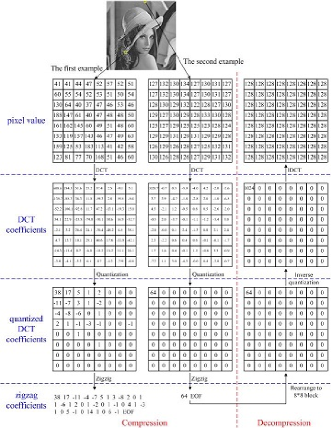
Figure 5: Two examples about the JPEG compression.

2.3 Quantum multiplier and quantum adder

Section 2.2 tells us that two operations: multiplication and addition are used in JPEG compression and decompression. Hence, we use the quantum multiplier [17] and the quantum adder [18] to realize them respectively.

The quantum multiplier and the quantum adder are both quantum networks, which can calculate the product or the sum of two numbers which are stored in two $n$-qubit quantum registers $|a\rangle$ and $|b\rangle$, where $a=|a_{n-1}a_{n-2}\cdots a_{0}\rangle$ and $b=|b_{n-1}b_{n-2}\cdots b_{0}\rangle$.

The quantum multiplication operation $M$ is

$$M(|a\rangle,|b\rangle,|0\rangle^{\otimes 2n})=(|a\rangle,|b\rangle,|a\times b\rangle)$$ (9)

and the quantum addition operation $A$ is

$$A(|a\rangle,|b\rangle)=(|a\rangle,|a+b\rangle)$$ (10)

where, $|a\times b\rangle$ is a $2n$-qubit quantum register and $|a+b\rangle$ is a $(n+1)$-qubit quantum register.

In the following, we use “MULER” and “ADDER” to represent the quantum multiplier and the quantum adder respectively as shown in Fig. 6.

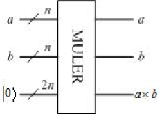
(a) The quantum multiplier

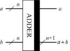
(b) The quantum adder

Figure 6: The quantum multiplier and the quantum adder.

According to Ref. [17] and [18], the complexity of MULER is

$$\begin{split}&n^{2}\text{ (2)-CNOT gates}+\sum_{l=1}^{\log_{2}n}\text{the complexity of Stage }l\\ =&n^{2}+\sum_{l=1}^{\log_{2}n}(4n+4l+4\cdot 2^{l-1}-10)\\ =&n^{2}+4n-4+(4n-8+2\log_{2}n)\log_{2}n\end{split}$$ (11)

The complexity of ADDER is

$$\begin{split}&(2n-1)\text{ Carry modules}+n\text{ Sum modules}+1\text{ CNOT gate}\\ =&3(2n-1)+2n+1\\ =&8n-2\end{split}$$ (12)

Note that

1. In Fig. 6(b), there has a thick black bar on the right-hand side of the quantum adder. A network with a bar on the left side represents the reversed sequence of elementary gates embedded in the same network with the bar on the right side. If the action of the quantum adder is reversed with the input $(a,b)$, the output will output $(a,b-a)$ when $b\geq a$. When $b<a$, the output is $(a,2^{n}-(a-b))$.

2. Ref. [17] said that Stage $l$ had $\frac{n}{2^{l}}$ ripple quantum adders with size $n+l+2^{l-1}-2$ in parallel. Since the $\frac{n}{2^{l}}$ ripple quantum adders work at the same time, the time required to run all the $\frac{n}{2^{l}}$ ripple quantum adders is equal to the run time of one ripple quantum adder. That is to say the time complexity of State $l$ is equal to one ripple quantum adder.

3. The ripple quantum adder is different from the quantum adder given in Ref. [18]. The time complexity of a ripple quantum adder with size $n$ is $4n-2$. Hence, the complexity of a ripple quantum adder with size $n+l+2^{l-1}-2$ is $4n+4l+4\cdot 2^{l-1}-10$.

4. Due to the length limitation of this paper, to get more details about MULER and ADDER, please refer to Ref. [17] and [18].

3 Quantum JPEG image compression

3.1 Basic idea

Unlike the existed schemes that store pixel values in quantum computers directly, the basic idea of our scheme is to store quantized DCT coefficients into qubits and then transform them into pixel values. Due to the volume of DCT coefficients is obviously smaller than the volume of pixel values, the complexity of preparation is decreased, i.e., the quantum image is compressed. Fig. 7 gives a schematic diagram to contrast our scheme with traditional schemes.

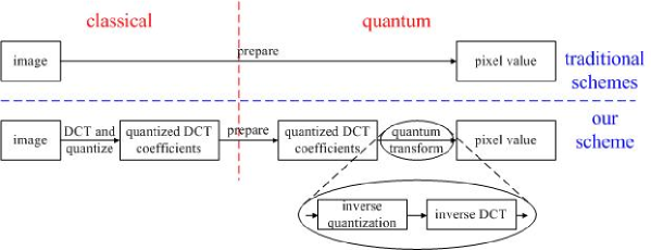
Figure 7: The basic idea of our scheme and the contrast with traditional schemes.

Note that the zigzag step is no longer needed in our scheme because the quantized coefficients are input into quantum computers in the form of $8\times 8$ blocks directly.

Section 2.2.2 tells us that when transform the quantized DCT coefficients into pixel values, it needs two steps: multiply each $8\times 8$ block with the quantization matrix $Q$ (inverse quantization), and do inverse DCT (IDCT) to each $8\times 8$ block to get the recovered pixel value $f^{\prime}(i,j)$.

Based on the unitarity of quantum algorithms, quantum IDCT can be realized by simply reverse the order of logic gates in quantum DCT algorithms. However the existed quantum DCT algorithms [19-20] is not suitable to our scheme because their data storage format is different from ours:

1. Ref. [19-20] use $d=Uc$ to do quantum DCT, where $c=[c_{0}\ c_{1}\ \cdots\ c_{2^{n}-1}]^{\text{T}}$ is the space domain data (i.e., the original pixel values), $d=[d_{0}\ d_{1}\ \cdots\ d_{2^{n}-1}]^{\text{T}}$ is the frequency domain data (i.e., the DCT coefficients), and $U$ is the quantum DCT transformation. Hence, the pixels and the coefficients are stored as the probability of basic states.

2. Our scheme converts the pixel values and the coefficients to binary strings and use the corresponding basic states to represent them. The probabilities of all the corresponding basic states are the same.

Hence, the quantum DCT and IDCT method proposed in Ref. [19-20] can not be utilized in this paper. We will give a new way to realize quantum IDCT and describe it in the next subsection.

3.2 Quantum JPEG image compression algorithm

For the sake of simplicity, we assume that the size of the image is $2^{n}\times 2^{n}$.

1. DCT and quantize.

It is a preprocessing step done in classical computers as described in Step 1 and 2 of Section 2.2.1.

1. Store the quantized DCT coefficients into quantum systems.

It is similar to the GQIR preparation stated in Section 2.1.

Initially, $q+2n$ qubits are prepared and set to $|0\rangle$. The initial state can be expressed as in

$$|\Psi_{0}\rangle=|0\rangle^{\otimes q+2n}$$ (13)

Then, $q$ identity gates and $2n$ Hadamard gates are used to construct a $2^{n}\times 2^{n}$ blank image. The identity matrix and the Hadamard matrix are shown below.

$$I=\left[\begin{array}[]{cc}1&0\\ 0&1\end{array}\right]\ \ \ \ H=\frac{1}{\sqrt{2}}\left[\begin{array}[]{cc}1&1\\ 1&-1\end{array}\right]$$ (14)

The whole quantum operation in this step can be expressed as $U_{2.1}$:

$$U_{2.1}=I^{\otimes q}\otimes H^{\otimes 2n}$$ (15)

$U_{2.1}$ transforms the initial state $|\Psi_{0}\rangle$ to the state $|\Psi_{1}\rangle$.

$$\begin{split}|\Psi_{1}\rangle&=U_{2.1}(|\Psi_{0}\rangle)=(I|0\rangle)^{\otimes q}\otimes(H|0\rangle)^{\otimes 2n}\\ &=\frac{1}{2^{n}}|0\rangle^{\otimes q}\otimes\sum_{i=0}^{2^{2n}-1}|i\rangle\\ &=\frac{1}{2^{n}}\sum_{Y=0}^{2^{n}-1}\sum_{X=0}^{2^{n}-1}|0\rangle^{\otimes q}|YX\rangle\end{split}$$ (16)

In simple terms, the effect of identity gate is maintaining the qubit’s original state unchanged and the effect of Hadamard gate is letting state $|0\rangle$ and state $|1\rangle$ appear with equal probability. Note that because identity gates $I$ remain qubit’s state unchanged, they can be omitted. After $U_{2.1}$, the blank $2^{n}\times 2^{n}$ image is gained.

Next, store the quantized DCT coefficients. It is divided into $2^{n-3}\times 2^{n-3}\times 64=2^{2n}$ sub-operations and each sub-operation stores one quantized DCT coefficient, where $2^{n-3}\times 2^{n-3}$ is the number of $8\times 8$ blocks and 64 indicates that there are 64 coefficients to be stored in each block. We still use $X$ and $Y$ to distinguish sub-operations. For the $(u,v)$th sub-operation in block $(i,j)$, we have

$$\begin{split}&X=8j+v\\ &Y=8i+u\end{split}$$ (17)

In general, in each block, $F_{Q}(0,0)$ is the biggest coefficient of all $F_{Q}(u,v)$, $u=0,\cdots,7$, $v=0,\cdots,7$. Due to

$$F_{Q}(0,0)=round\left(\frac{F(0,0)}{Q(0,0)}\right)=round\left(\frac{1}{16}\times\frac{1}{8}\sum_{i=0}^{7}\sum_{j=0}^{7}f(i,j)\right)$$

and $f(i,j)$ does not exceed $2^{q}-1$,

$$F_{Q}(0,0)<round\left(\frac{1}{16}\times\frac{1}{8}\times 64\left(2^{q}-1\right)\right)=2^{q-1}.$$

Note that there is a special item. When all $f(i,j)=2^{q}-1$,

$$round\left(\frac{1}{16}\times\frac{1}{8}\times 64\left(2^{q}-1\right)\right)=round(2^{q-1}-0.5)=2^{q-1}.$$

However, JPEG compression defines that the quantization result of the special item is $2^{q-1}-1$.

Hence, $q-1$ qubits are enough to store $F_{Q}(u,v)$. However, sometimes, $F_{Q}(u,v)$ may be a negative number. The most significant qubit is used as the sign position: if $F_{Q}(u,v)$ is a negative number, the most significant qubit is set to state $|1\rangle$; and if $F_{Q}(u,v)$ is a positive number, the most significant qubit remains state $|0\rangle$.

The quantum sub-operation $U_{YX}$ is shown below.

$$U_{YX}=\left(I\otimes\sum_{ji\neq YX}|ji\rangle\langle ji|\right)+\Omega_{YX}\otimes|YX\rangle\langle YX|$$ (18)

where $\Omega_{YX}$ is the quantum operation to transform the value of pixel $(Y,X)$ from $|0\rangle^{\otimes q}$ to the desired quantized DCT coefficient as shown in Eq. (19). Hence, the function of $U_{YX}$ is change pixel $(Y,X)$ and others remain unchanged.

$$\Omega_{YX}=\bigotimes_{i=0}^{q-1}\Omega_{YX}^{i}$$ (19)

The function of $\Omega_{YX}^{i}$ is setting the value of the $i$th qubit of pixel $(Y,X)$’s quantized DCT coefficient.

$$\Omega_{YX}^{i}:|0\rangle\rightarrow|0\oplus C_{YX}^{i}\rangle$$ (20)

where $\oplus$ is the XOR operation. If $C_{YX}^{i}=1$, $\Omega_{YX}^{i}:|0\rangle\rightarrow|1\rangle$ is a $2n$-CNOT gate (a CNOT gate with $2n$ control qubits). Otherwise, $\Omega_{YX}^{i}:|0\rangle\rightarrow|0\rangle$ is a quantum identity gate which will do nothing on the quantum state. Hence,

$$\Omega_{YX}|0\rangle^{\otimes q}=\bigotimes_{i=0}^{q-1}(\Omega_{YX}^{i}|0\rangle)=\bigotimes_{i=0}^{q-1}|0\oplus C_{YX}^{i}\rangle=\bigotimes_{i=0}^{q-1}|C_{YX}^{i}\rangle=|C_{YX}\rangle$$ (21)

Act $U_{YX}$ on $|\Psi_{1}\rangle$

$$\begin{split}U_{YX}(|\Psi_{1}\rangle)&=U_{YX}\left(\frac{1}{2^{n}}\sum_{j=0}^{2^{n}-1}\sum_{i=0}^{2^{n}-1}|0\rangle^{\otimes q}|ji\rangle\right)\\ &=\frac{1}{2^{n}}U_{YX}\left(\sum_{ji\neq YX}|0\rangle^{\otimes q}|ji\rangle+|0\rangle^{\otimes q}|YX\rangle\right)\\ &=\frac{1}{2^{n}}\left(\sum_{ji\neq YX}|0\rangle^{\otimes q}|ji\rangle+\Omega_{YX}|0\rangle^{\otimes q}|YX\rangle\right)\\ &=\frac{1}{2^{n}}\left(\sum_{ji\neq YX}|0\rangle^{\otimes q}|ji\rangle+|C_{YX}\rangle|YX\rangle\right)\end{split}$$ (22)

$U_{YX}$ only sets the quantized DCT coefficient of its corresponding pixel. In order to set all the $2^{n}\times 2^{n}$ pixels, a quantum operation $U_{2.2}$ is defined below.

$$U_{2.2}=\prod_{\begin{subarray}{c}X=0,\cdots,2^{n}-1\\ Y=0,\cdots,2^{n}-1\end{subarray}}U_{YX}$$ (23)

Act $U_{2.2}$ to $|\Psi_{1}\rangle$

$$|\Psi_{2}\rangle=U_{2.2}(|\Psi_{1}\rangle)=\frac{1}{2^{n}}\sum_{\begin{subarray}{c}X=0,\cdots,2^{n}-1\\ Y=0,\cdots,2^{n}-1\end{subarray}}|C_{YX}\rangle|YX\rangle$$ (24)

In simple terms, the effect of Step 2 is using $2n$ Hadamard gates and $2n$-CNOT gates to store the quantized DCT coefficients to a quantum system. The number of $2n$-CNOT gates is equal to the number of “1” in binary coefficients plus the number of negative coefficients.

1. Store the quantization matrix.

This step uses the similar method as the previous step to store the quantization matrix $Q$ (shown in Eq. (5)) into qubits: 1) $(q-1)+6=q+5$ qubits are prepared and set to $|0\rangle$. 2) 6 Hadamard gates are used to construct a $8\times 8$ blank matrix. 3) Some 6-CNOT gates are used to set the value of $Q$.

Due to $Q$ is a $8\times 8$ matrix, the CNOT gates used in this step have 6 control qubits. After Step 3, the quantum quantization matrix is:

$$\begin{split}|Q\rangle=&\sum_{Y_{Q}=0}^{7}\sum_{X_{Q}=0}^{7}|Q_{Y_{Q}X_{Q}}\rangle\otimes|Y_{Q}X_{Q}\rangle\\ =&|16\rangle|000000\rangle+|11\rangle|000001\rangle+|10\rangle|000010\rangle+|16\rangle|000011\rangle\\ &+\cdots+\\ &+|112\rangle|111100\rangle+|100\rangle|111101\rangle+|103\rangle|111110\rangle+|99\rangle|111111\rangle\end{split}$$ (25)

where, in the second to fourth line, $Q_{Y_{Q}X_{Q}}$ is given in decimal and $Y_{Q}X_{Q}$ is given in binary.

1. Inverse quantization.

We use MULER to multiply each $8\times 8$ block with the quantization matrix $|Q\rangle$ as Eq. (7) shows. The multiplication is element-by-element: only when $|Y_{Q}X_{Q}\rangle=|Y_{2}Y_{1}Y_{0}X_{2}X_{1}X_{0}\rangle$, MULER is used to multiply the coefficient block and the quantization matrix, where $Y_{Q}X_{Q}$ is the location information of the quantization matrix and $Y_{2}Y_{1}Y_{0}X_{2}X_{1}X_{0}$ is part of the location information of the DCT coefficient. That is to say, each element in the quantization matrix is multiplied with the corresponding DCT coefficients in each $8\times 8$ block.

Step 4 can be broken down into the following steps.

1. Judge whether $|Y_{Q}X_{Q}\rangle=|Y_{2}Y_{1}Y_{0}X_{2}X_{1}X_{0}\rangle$.

   Define

   $$U_{4.1}^{i,T}:|T_{Qi},T_{i}\rangle\rightarrow|T_{Qi}\oplus T_{i},T_{i}\rangle$$ (26)

   where $T\in\{Y,X\}$, $i\in\{0,1,2\}$. That is to say, $U_{4.1}^{i,T}$ is a CNOT gate: if $T_{Qi}=T_{i}$, $T_{Qi}$ is changed to 0; otherwise, $T_{Qi}$ is changed to 1. Hence, by acting

   $$U_{4.1}=\bigotimes_{\begin{subarray}{c}i=0,1,2\\ T=Y,X\end{subarray}}U_{4.1}^{i,T}$$ (27)

   to state $|\Psi_{2}\rangle\otimes|Q\rangle$, we can align $8\times 8$ blocks with $|Q\rangle$, i.e., if all the $|T_{Qi}\oplus T_{i}\rangle$ is equal to $|0\rangle$, each element in the quantization matrix finds its corresponding DCT coefficients in each $8\times 8$ block. For the sake of simplicity, when no ambiguity is possible, we still use $|T_{Qi}\rangle$ to substitute $|T_{Qi}\oplus T_{i}\rangle$.

2. If the condition is satisfied (i.e., all the $|T_{Qi}\rangle$ is equal to $|0\rangle$), change the state of a auxiliary qubit $|g\rangle$ with initial state $|0\rangle$ to $|1\rangle$.

   A transform $U_{4.2}$ is defined.

   $$U_{4.2}:|g=0\rangle\rightarrow|g=1\rangle\text{, if }|Y_{Q}X_{Q}\rangle=|000000\rangle$$ (28)

   where, $U_{4.2}$ is a 6-CNOT gate.

3. If $|g=1\rangle$, multiply.

   $|g\rangle$ is the deliverable of Step 4.1 and 4.2. Hence, $|Y_{Q}X_{Q}\rangle$ has no use in the following and $|g\rangle$ substitutes them. If $|g=1\rangle$, we use MULER to multiply each $8\times 8$ block with the quantization matrix $|Q\rangle$ as Eq. (7) shows. We use $U_{4.3}$ to denote the operation.

   $$U_{4.3}:|F,Q,0\rangle\rightarrow|F,Q,F^{\prime}=F\times Q\rangle\text{, if }|g\rangle=|1\rangle$$ (29)

   Since the quantization matrix and the DCT coefficients are stored superposedly, one MULER is enough to multiply them parallel.

4. Transform the sign position.

   Define

   $$U_{4.4}:|F^{\prime 2(q-1)-1},F^{q-1}\rangle\rightarrow|F^{\prime 2(q-1)-1}\oplus F^{q-1},F^{q-1}\rangle\text{, if }|g\rangle=|1\rangle$$ (30)

   Hence, $U_{4.4}$ is a 2-CNOT gate: if $|g\rangle=|1\rangle$ and $|F^{q-1}\rangle=|1\rangle$, the sign position $|F^{\prime 2(q-1)-1}\rangle$ in $|F^{\prime}\rangle$ is changed to $|1\rangle$.

Fig. 8 gives the circuit of Step 4. When $|g\rangle=|1\rangle$, the subspace $|F^{\prime}\rangle\otimes|YX\rangle$ stores the recovered DCT coefficients.

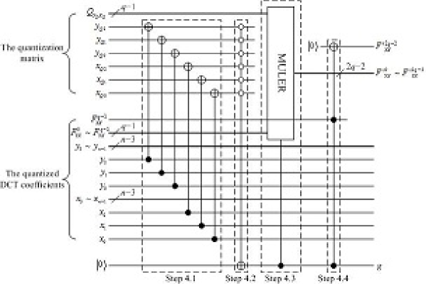
Figure 8: Step 4: inverse quantization.

1. Inverse DCT.

In Eq. (8), $c(u)$, $c(v)$, $\cos\left[\frac{(i+0.5)\pi}{8}u\right]$ and $\cos\left[\frac{(j+0.5)\pi}{8}v\right]$ are independent from image. We see them as a whole. Hence, Eq. (8) can be changed into

$$\begin{split}f^{\prime}(i,j)=&\sum_{u=0}^{7}\sum_{v=0}^{7}\left\{c(u)c(v)F^{\prime}(u,v)\cos\left[\frac{(i+0.5)\pi}{8}u\right]\cos\left[\frac{(j+0.5)\pi}{8}v\right]\right\}\\ =&\sum_{u=0}^{7}\sum_{v=0}^{7}\left\{F^{\prime}(u,v)\times C_{ij}(u,v)\right\}\end{split}$$ (31)

where $C_{ij}(u,v)=c(u)c(v)\cos\left[\frac{(i+0.5)\pi}{8}u\right]\cos\left[\frac{(j+0.5)\pi}{8}v\right]$.

Therefore, this step is divided into two main parts: multiply $F^{\prime}(u,v)$ with $C_{ij}(u,v)$ and add all the 64 products up.

1. Store $C_{ij}(u,v)$.

   This step uses the similar method as Step 2 to store $C$ into qubits: 1) $64(q+4)+6=64q+262$ qubits are prepared and set to $|0\rangle$. 2) 6 Hadamard gates are used to construct $i$ and $j$. 3) Some 6-CNOT gates are used to set the value of $C$.

   Although $|F^{\prime}_{YX}\rangle\otimes|YX\rangle$ use $2q-1$ qubits to represent the value of DCT coefficients, only $q+4$ qubits works. That is because in a $8\times 8$ block, the max value of $F^{\prime}(u,v)$ is $F^{\prime}(0,0)$, and

   $$F^{\prime}(0,0)=F_{Q}(0,0)\times Q(0,0)=16F_{Q}(0,0)<16\cdot 2^{q-1}=2^{q+3}$$

   Therefore we only take the first $q+3$ qubits ($F_{YX}^{{}^{\prime}q-5}\sim F_{YX}^{{}^{\prime}2q-3}$) to participate in the following steps. $F_{YX}^{{}^{\prime}2q-2}$ still is the sign. In order to multiply $F^{\prime}$ with $C$ using MULER, we also use $q+3$ qubits to store the value of $C_{ij}(u,v)$ and $C_{ij}^{q+3}(u,v)$ is the sign position.

   $C_{ij}(u,v)$ has up to $8^{4}=4096$ values because $i,j,u,v\in\{0,1,\cdots,6,7\}$. By calculating all of them, we find that

   $$-0.2405\leq C_{ij}(u,v)\leq 0.2405$$ (32)

   Hence, except the sign qubit $C_{ij}^{q+3}(u,v)$, other $q+3$ qubits store the fractional part of the absolute value.

   That is to say, each $C_{ij}(u,v)$ uses $q+4$ qubits to store. However, because $u,v\in\{0,1,2,3,4,5,6,7\}$, $64(q+4)$ qubits are needed to store all $C_{ij}(u,v)$.

2. Multiply the absolute value of $F^{\prime}(u,v)$ with $C_{ij}(u,v)$.

   Define

   $$\begin{split}U_{5.2}^{u,v}:&|F^{\prime}(u,v),C_{ij}(u,v)\rangle\\ \rightarrow&|P^{2q+5}_{ij}(u,v)\cdots P^{0}_{ij}(u,v)\rangle=|F^{\prime}(u,v)\times C_{ij}(u,v)\rangle\end{split}$$ (33)

   It is a quantum multiplier MULER with 6 control qubits: $|y_{2}y_{1}y_{0}\rangle$ and $|x_{2}x_{1}x_{0}\rangle$ are the control qubits, and if the binary values $y_{2}y_{1}y_{0}=u$ and $x_{2}x_{1}x_{0}=v$, MULER works. Due to the absolute values of $F^{\prime}(u,v)$ and $C_{ij}(u,v)$ both occupy $q+3$ qubits, the result occupies $2q+6$ qubits.

   Use 64 MULERs

   $$U_{5.2}=\bigotimes_{\begin{subarray}{c}u=0,\cdots,7\\ v=0,\cdots,7\end{subarray}}U_{5.2}^{u,v}$$ (34)

   to multiply all $F^{\prime}(u,v)$ with $C_{ij}(u,v)$.

   Symbol $P_{ij}(u,v)$ is used to denote the product of $F^{\prime}(u,v)$ and $C_{ij}(u,v)$. Since $F^{\prime}(u,v)$ is a $(q+3)$-qubit integer and $C_{ij}(u,v)$ is a $(q+3)$-qubit pure decimal, the higher $q+3$ qubits of $P_{ij}(u,v)$ are the integer part and the lower $q+3$ qubits are the fractional part.

3. Set the sign position.

   Define

   $$\begin{split}U_{5.3}^{u,v}:&|0\rangle\rightarrow|1\rangle\text{, if }y_{2}y_{1}y_{0}=u\text{ and }x_{2}x_{1}x_{0}=v\\ &\text{ and }((F^{{}^{\prime}2q-2}(u,v)=1\text{ and }C^{q+3}_{ij}(u,v)=0)\\ &\text{ or }(F^{{}^{\prime}2q-2}(u,v)=0\text{ and }C^{q+3}_{ij}(u,v)=1))\end{split}$$ (35)

   It is a 8-CNOT gate: if the sign position of $F^{\prime}(u,v)$ is different with the sign position of $C_{ij}(u,v)=1$, and $y_{2}y_{1}y_{0}=u$ and $x_{2}x_{1}x_{0}=v$, change the new sign position $|P^{2q+6}_{ij}(u,v)\rangle$ from $|0\rangle$ to $|1\rangle$.

   Define

   $$U_{5.3}=\bigotimes_{\begin{subarray}{c}u=0,\cdots,7\\ v=0,\cdots,7\end{subarray}}U_{5.3}^{u,v}$$ (36)

   to set all the 64 sign positions.

4. Add the 64 $|P_{ij}(u,v)\rangle$.

   According to Eq. (31), all the 64 $|P_{ij}(u,v)\rangle$ should be added together. We use 64 ADDER to realize it. Firstly, $|P^{2q+5}_{ij}(0,0)\cdots P^{0}_{ij}(0,0)\rangle$ and $|0\rangle^{\otimes 2q+6}$ are added. Then, $|P^{2q+5}_{ij}(u,v)\cdots P^{0}_{ij}(u,v)\rangle$ and the sum of the previous addition are added.

   However, there is a sign position $|P^{2q+6}_{ij}(u,v)\rangle$. If it is $|0\rangle$, $|P^{2q+5}_{ij}(u,v)$ $\cdots P^{0}_{ij}(u,v)\rangle$ should be added; if it is $|1\rangle$, $|P^{2q+5}_{ij}(u,v)\cdots P^{0}_{ij}(u,v)\rangle$ should be subtracted. Hence, $|P^{2q+6}_{ij}(u,v)\rangle$ is used as a control qubit: when $|P^{2q+6}_{ij}(u,v)\rangle=|0\rangle$, the thick black bar is on the right-hand hand of ADDER; otherwise, the thick black bar is on the left-hand hand of ADDER.

   The output of the last ADDER is the regained color information. It is denoted as $|f^{\prime 2q+5}\cdots f^{\prime 0}\rangle$ and the higher $q+3$ qubits are the integer part and the lower $q+3$ qubits are the fractional part. However, GQIR only uses $q$ qubits to represent color. Hence, only the lower $q$ qubits of the integer part is useful. It is $|f^{\prime 2q+2}\cdots f^{\prime q+3}\rangle$.

Fig. 9 gives the circuit of Step 5. The useful output of Step 5 is $|f^{\prime 2q+2}\cdots$ $f^{\prime q+3}\rangle\otimes|y_{n-1}\cdots y_{3}i_{2}i_{1}i_{0}x_{n-1}\cdots x_{3}j_{2}j_{1}j_{0}\rangle$ and it is the GQIR image. $|f^{\prime 2q+2}\cdots$ $f^{\prime q+3}\rangle$ is the color information and $|y_{n-1}\cdots y_{3}i_{2}i_{1}i_{0}x_{n-1}\cdots x_{3}j_{2}j_{1}j_{0}\rangle$ is the location information.

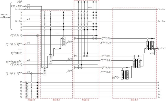
Figure 9: Step 5: inverse DCT.

4 Network complexity and compression ratio

In this section, we will compare our scheme with GQIR preparation and BEC method to highlight the advantages of our scheme. However, our scheme and BEC have a preprocessing step done in classical computers. As we all know, classical computers and quantum computers have different physical principles. Hence, we will compare the quantum part and the classical part separately.

4.1 Quantum part

The network complexity depends very much on what is considered to be an elementary gate. This is a problem about gate granularity. For example, one Toffoli gate (a NOT gate with 2 control qubits) can be simulated by six Control-NOT gates (a NOT gate with 1 control qubits) [18]. However, in this paper, we take one gate can be drawn in a quantum circuit as an elementary gate, no matter how many control qubits it has and what function it finishes.

The GQIR preparation is done in quantum computers. From Section 2.1, we know that the complexity of the GQIR preparation is equal to the number of bit 1 in all the pixels. By assuming that every bit has equal probability to be 0 or 1, then the GQIR preparation complexity before compression is

$$C=\frac{1}{2}2^{n}\times 2^{n}\times q=\frac{q}{2}2^{2n}$$ (37)

We will give our scheme’s complexity based on $C$.

To our scheme, only Step 2-5 are analyzed because the scope of Section 4.1 is quantum part.

The complexity of Step 2 (The number of gates used in Step 2) in our scheme is equal to the number of bit 1 plus the number of negatives in all the coefficients. We define it as

$$r_{J}\cdot C$$ (38)

where,

$$\begin{split}r_{J}&=\frac{\text{(The number of bit 1}+\text{the number of negatives) in all the coefficients}}{\text{The number of bit 1 in all the pixels}}\\ &=\frac{\text{The complexity after compression}}{\text{The complexity before compression}}\end{split}$$ (39)

is called JPEG compression ratio. We use statistical method to gain $r_{J}$. 800 images obtained from Washington University [21], University of South California [22] and Pixabay [23] are used, including people, animals, streetscape, buildings, natural beauty, remote sensing, texture, man-made pattern, and so on. These images almost cover all common image types. Fig. 10 gives some samples.

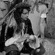
(a) people

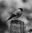
(b) animal

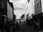
(c) streetscape

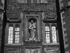
(d) building

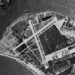
(e) remote sensing

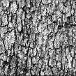
(f) texture

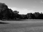
(g) natural beauty

(h) man-made pattern

Figure 10: Samples from the image database (the 800 images) which contains a large range of image types.

We calculate each image’s compression ratio $r_{J}$ and show it in Fig. 11. The maximum value is 0.2364, the minimum value is 0.0148, the average value is 0.0934, and the variance is only 0.0014. Hence, in the following, we set

$$r_{J}=0.1$$ (40)

and the complexity of Step 2 is

$$C_{2}=0.1\cdot\frac{q}{2}2^{2n}=\frac{q}{20}2^{2n}$$ (41)

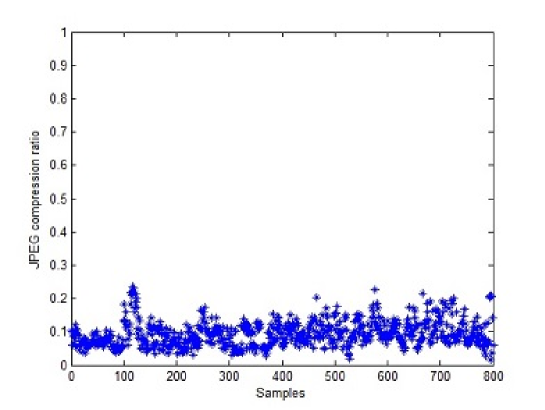
Figure 11: The statistical JPEG compression ratio of the 800 images.

Step 3 is used to store the quantization matrix. Since the quantization matrix is fixed as Eq. (5) shows, the complexity of Step 3 (The number of gates used in Step 3) is also fixed. It is equal to the number of bit 1 in all the quantization values. Hence,

$$C_{3}=208$$ (42)

The complexity of Step 4 (The number of gates used in Step 4) is also fixed.

$$\begin{split}C_{4}=&\text{6 CNOT gates}+\text{1 (6)-CNOT gate}+\text{1 MULERs}+\text{1 (2)-CNOT gate}\\ =&6+1+(q-1)^{2}+4(q-1)+4+\left(4(q-1)-8+2\log_{2}(q-1)\right)\log_{2}(q-1)\\ &+1\\ =&q^{2}+2q+9+\left(4q-12+2\log_{2}(q-1)\right)\log_{2}(q-1)\end{split}$$ (43)

The complexity of Step 5 (The number of gates used in Step 5) is

$$\begin{split}C_{5}=&\text{The number of bit 1 in all }C_{ij}(u,v)+\text{64 MULERs}\\ &+\text{128 (8)-CNOT gates}+\text{128 ADDERs}\\ =&\frac{q+4}{2}64+64\left[(q+3)^{2}+4(q+3)-4\right.\\ &\left.+\left(4(q+3)-8+2\log_{2}(q+3)\right)\log_{2}(q+3)\right]+128+128(8(2q+6)-2)\\ =&64q^{2}+2720q+7232+64(4q+4+2\log_{2}(q+3))\log_{2}(q+3)\end{split}$$ (44)

Note that the first item in the third line in Eq. (44) is $\frac{q+4}{2}64$. That is because: 1) $C_{ij}(0,0),\cdots,C_{ij}(7,7)$ have 64 components; 2) each $C_{ij}(u,v)$ is composed by $q+4$ qubits; and 3) each qubit has equal probability to be 0 and 1.

Hence, the complexity of compressed preparation is

$$\begin{split}&C_{2}+C_{3}+C_{4}+C_{5}\\ =&\frac{2^{2n}}{20}q+65q^{2}+2722q+7449+(4q-12+2\log_{2}(q-1))\log_{2}(q-1)\\ &+64(4q+4+2\log_{2}(q+3))\log_{2}(q+3)\end{split}$$ (45)

If our scheme compresses the image preparation,

$$C_{2}+C_{3}+C_{4}+C_{5}<C$$

i.e.,

$$\begin{split}&\frac{2^{2n}}{20}q+65q^{2}+2722q+7449+(4q-12+2\log_{2}(q-1))\log_{2}(q-1)\\ &+64(4q+4+2\log_{2}(q+3))\log_{2}(q+3)<\frac{q}{2}2^{2n}\end{split}$$

Hence, when

$$n>\frac{1}{2}\log_{2}\frac{65q^{2}+2722q+7449+A+B}{0.45q},$$ (46)

where $A=(4q-12+2\log_{2}(q-1))\log_{2}(q-1)$ and $B=64(4q+4+2\log_{2}(q+3))\log_{2}(q+3)$, our scheme can compress the quantum image preparation.

Assume that

$$m=\frac{1}{2}\log_{2}\frac{65q^{2}+2722q+7449+A+B}{0.45q}$$

is a function of $q$. The function image is shown in Fig. 12, in which $q$ is ranged from 4 to 40 to cover almost all the color depth used in JPEG compression.

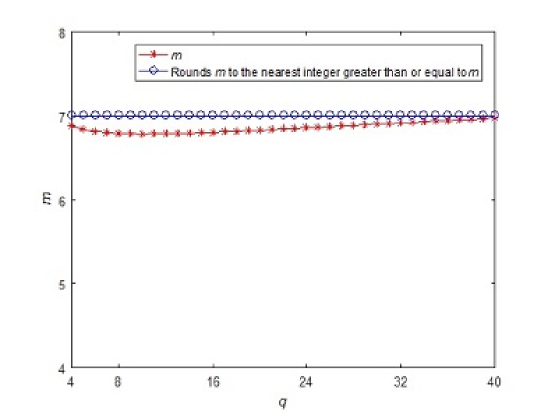
Figure 12: The relationship between the color depth $q$ and the $m$. Because $n$ is a positive integer, we also round $m$ to the nearest integer greater than or equal to $m$. That is to say, the line with small circles gives the lowest value of $n$.

Fig. 12 tells us that as long as the image size is bigger than $2^{7}\times 2^{7}=128\times 128$, our scheme can compress the image. It is a easy to achieve requirement because most of the common image sizes are bigger than $128\times 128$.

Definition 1

Quantum image compression ratio

$$r=1-\frac{\text{The number of operations after compression}}{\text{The number of operations before compression}}$$

Due to

$$r=1-\frac{C_{2}+C_{3}+C_{4}+C_{5}}{C},$$

the compression ratio of our scheme is

$$r=1-\frac{\frac{2^{2n}}{20}q+65q^{2}+2722q+7449+A+B}{\frac{q}{2}2^{2n}}$$ (47)

Fig. 13 gives the $r$ changed with $n$ and $q$. It tells us that:

1. No matter how much the value of $q$, when $n\geq 10$, i.e., the image size is equal to or bigger than $1024\times 1024$, $r$ is approximately 0.9. That is to say, the JPEG complexity is only $\frac{1}{10}$ of the original complexity.

2. The bigger the $n$, the higher the compression ratio $r$.

The reason to these two items is that

$$r=1-\frac{C_{2}+C_{3}+C_{4}+C_{5}}{C}=0.9-\frac{C_{3}+C_{4}+C_{5}}{\frac{q}{2}2^{2n}}$$

and $C_{3}$, $C_{4}$ and $C_{5}$ are independent of $n$, hence as $n$ increases, $r$ increases rapidly and the limit is 0.9.

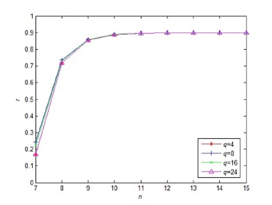
Figure 13: The quantum image compression ratio $r$ is changed with the image size $n$ and color depth $q$.

We also compare the compression ratio of our scheme with BEC in Table 1. However, as stated in Section 2.1, if the preprocessing is taken into account, BEC’s complexity is too high to bear. Hence, we only test 3 $256\times 256$ images with $q=8$. It can be seen that our scheme’s compression ratio is higher than that of BEC scheme.

Table 1: The compression ratio (not include preprocessing).

Image	Compression ratio		The number of operations after/before compression (GQIR)
	our scheme (JPEG)	BEC	our scheme (JPEG)	BEC
Cameraman	84.66%	69.07%	37638/245366	75901/245366
Lena	85.09%	66.17%	38450/257833	87217/257833
Baboon	67.58%	66.00%	89911/277344	94307/277344

4.2 Classical part

Our scheme and BEC have a preprocessing step done in classical computers.

From Eq. (4) and (6), it is obvious that the complexity of DCT and quantization are both $O(2^{2n})$. Hence, the preprocessing complexity of our scheme is $O(2\cdot 2^{2n})$. From Eq. (3), the preprocessing complexity of BEC is $O(2n\cdot q\cdot 2^{4n})$.

$$O(2n\cdot q\cdot 2^{4n})\gg O(2\cdot 2^{2n})$$

Furthermore, there are fast algorithms for DCT which can improve the efficiency [24]. Fast DCT has been widely used in classical image compression. When you use your phone to take a picture, you do DCT one time because the picture has been compressed and its filename extension is “jpg”. We do not plane to describe fast DCT theoretically as the length limit of the paper. However, some data are given to compare our scheme and BEC intuitively (see Table 2). The experiment environment is a desktop with Intel(R) Core(TM) i5-4590 CPU 3.3GHz, 8GB Ram equipped with MATLAB R2016b.

Table 2: The preprocessing time ($q=8$).

image name	$n$	image size	our scheme	BEC
Cameraman	8	$256\times 256$	0.176 second	—
Lena	8	$256\times 256$	0.164 second	5.54 hour
Baboon	8	$256\times 256$	0.164 second	—
Cameraman	9	$512\times 512$	0.516 second	—
Lena	9	$512\times 512$	0.505 second	more than 3 days
Baboon	9	$512\times 512$	0.505 second	—

Note: 1) “—” indicates that we do not do that experiment. 2) “more than 3 days” because the experiment has been done for 3 days but has not been finished, so we stopped it.

It is obviously that our scheme is faster than BEC.

5 Visual effects

Unlike GQIR preparation and BEC, our scheme is a lossy method which may affect the quality of the image. However, JPEG can help us to ensure the visual quality of the images. In this section, some examples are given to display the visual effects.

Due to the condition that the physical quantum hardware is not affordable for us to execute our protocol, we just make the simulations on the classical computer mentioned in Section 4.2.

Fig. 14 gives the visual effects of our scheme.

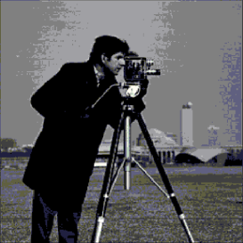
(a) uncompressed cameraman

(b) compressed cameraman

(c) uncompressed Lena

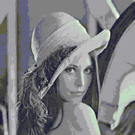
(d) compressed Lena

(e) uncompressed baboon

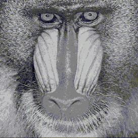
(f) compressed baboon

Figure 14: Visual effects of our scheme. Images in the left are uncompressed and images in the right are compressed.

The peak-signal-to-noise ratio (PSNR), being one of the most used quantity in classical for comparing the fidelity of two images, will be used to evaluate the quality of the compressed images. By assuming $I$ and $I^{\prime}$ are two $2^{n}\times 2^{n}$ images, the PSNR is defined by

$$\text{PSNR}=20\log_{10}\left(\frac{MAX_{I}}{\sqrt{\frac{1}{2^{4n}}\sum_{i=0}^{2^{n}-1}\sum_{j=0}^{2^{n}-1}[I(i,j)-I^{\prime}(i,j)]}}\right)$$

where, $MAX_{I}$ is the maximum possible pixel value of the image. Table 3 gives the PSNR between images before and after compression.

Table 3: The PSNR values between images before and after compression.

image	PSNR
Cameraman	38.0683
Lena	35.7164
Baboon	27.9511

From Fig. 14 and Table 3, we can see that our scheme does not affect the images’ visual effect, and the PSNR is acceptable.

6 Conclusion

This paper focuses on quantum image preparation and gives a new quantum image compression scheme based on JPEG to prepare a GQIR image. Compared with BEC, our scheme has the following advantages:

1. Its preprocessing (DCT and quantization) is simple and fast.

2. As long as Eq. (46) is satisfied, its compression ratio is higher than that of BEC. Moreover, Eq. (46) is a loose condition because it requires that the size of the image is only bigger than or equal to $128\times 128$.

- (1) Venegas-Andraca S.E., Bose, S. Storing, processing and retrieving an image using quantum mechanics. Proceedings of the SPIE conference on Quantum Information and Computation, pp. 137-147 (2003)
- (2) Latorre, J.I.: Image compression and entanglement. arXiv:quant-ph/0510031 (2005)
- (3) Venegas-Andraca S.E., Ball J.L.: Processing images in entangled quantum systems. Quantum Information Processing 9(1), 1-11 (2010)
- (4) Le, P.Q., Dong, F.Y., Hirota, K.: A flexible representation of quantum images for polynomial preparation, image compression and processing operations. Quantum. Inf. Process. 10(1), 63-84 (2011)
- (5) Sun, B., Iliyasu, A.M., Yan, F., Dong, F.Y., Hirota, K.: An RGB multi-channel representation for images on quantum computers. Journal of Advanced Computational Intelligence and Intelligent Informatics. 17(3), 404-417 (2013)
- (6) Zhang, Y., Lu, K., Gao, Y.H., Wang, M.: NEQR: a novel enhanced quantum representation of digital images. Quantum Inf. Process. 12(12), 2833-2860 (2013)
- (7) Zhang, Y., Lu, K., Gao, Y.H., Xu, K.: A novel quantum representation for log-polar images. Quantum Inf. Process. 12(9), 3103-3126 (2013)
- (8) Li, H.S., Zhu, Q.X., Lan, S., Shen, C.Y., Zhou, R.G., Mo, J.: Image storage, retrieval, compression and segmentation in a quantum system. Quantum Inf. Process, 12(6), 2269-2290 (2013)
- (9) Li, H.S., Zhu, Q.X., Zhou, R.G., Lan, S., Yang, X.J.: Multi-dimensional color image storage and retrieval for a normal arbitrary quantum superposition state. Quantum Inf. Process, 13(4), 991-1011 (2014)
- (10) Jiang, N., Wang, L.: Quantum image scaling using nearest neighbor interpolation. Quantum Inf. Process, 14(5), 1559-1571 (2015)
- (11) Jiang, N., Wang, J., Mu, Y.: Quantum image scaling up based on nearest-neighbor interpolation with integer scaling ratio. Quantum Inf. Process, 14(11), 4001-4026 (2015)
- (12) Yan, F., Iliyasu, A.M., Venegas-Andraca S.E.: A survey of quantum image representations. Quantum Inf. Process, 15(1), 1-35 (2016)
- (13) Jiang, N., Dang, Y.J., Wang, J.: Quantum image matching. Quantum Inf. Process, 15(9), 3543-3572 (2016)
- (14) Jiang, N., Dang, Y.J., Zhao, N.: Quantum image location. International Journal of Theoretical Physics, 55(10), 4501-4512 (2016)
- (15) Gonzalez, R.,Woods, R.: Digital Image Processing. Pearson/Prentice Hall, Upper Saddle River (2008)
- (16) https://cs.stanford.edu/people/eroberts/courses/soco/projects/data-compression/lossy/jpeg/lossless.htm
- (17) Saurabh Kotiyal, Himanshu Thapliyal, Nagarajan Ranganathan. Circuit for reversible quantum multiplier based on binary tree optimizing ancilla and garbage bits. 27th International Conference on VLSI Design and 13th International Conference on Embedded Systems: 545-550 (2014)
- (18) Vlatko, V., Adriano, B., Artur, E.: Quantum networks for elementary arithmetic operations. Phys. Rev. A 54(1), 147-153 (1996)
- (19) Klappenecker, A., Roetteler, M. Discrete cosine transforms on quantum computers. Proceedings of the 2nd International Symposium on Image and Signal Processing and Analysis, 464-468 (2001)
- (20) Tseng, C., Hwang, T. Quantum circuit design of discrete cosine transform using its fast computation flow graph. IEEE International Symposium on Circuits and Systems, 1: 828-831 (2005)
- (21) http://imagedatabase.cs.washington.edu/ (2016)
- (22) http://sipi.usc.edu/services/database/index.html (2016)
- (23) https://pixabay.com (2016)
- (24) Ephraim Feig, Shmuel Winograd. Fast algorithms for the discrete Cosine transform. IEEE Transactions on Signal Processing, 40(9): 2174-2193 (1992)