Quark orbital dynamics in the proton from Lattice QCD – from Ji to Jaffe-Manohar orbital angular momentum

Abstract

Given a Wigner distribution simultaneously characterizing quark transverse positions and momenta in a proton, one can directly evaluate their cross-product, i.e., quark orbital angular momentum. The aforementioned distribution can be obtained by generalizing the proton matrix elements of quark bilocal operators which define transverse momentum-dependent parton distributions (TMDs); the transverse momentum information is supplemented with transverse position information by introducing an additional nonzero momentum transfer. A gauge connection between the quarks must be specified in the quark bilocal operators; the staple-shaped gauge link path used in TMD calculations yields the Jaffe-Manohar definition of orbital angular momentum, whereas a straight path yields the Ji definition. An exploratory lattice calculation, performed at the pion mass $m_{\pi}=518\,\mbox{MeV}$, is presented which quasi-continuously interpolates between the two definitions and demonstrates that their difference can be clearly resolved. The resulting Ji orbital angular momentum is confronted with traditional evaluations based on Ji’s sum rule. Jaffe-Manohar orbital angular momentum is enhanced in magnitude compared to its Ji counterpart.

I Introduction

Decomposing the proton spin into the spin and orbital angular momentum contributions of its quark and gluon constituents has been a prominent endeavor of hadronic physics since the groundbreaking EMC experiments emc1 ; emc2 revealed that quark spin, by itself, does not account for the entirety of proton spin. In particular, quantifying the parton orbital dynamics already meets challenges at the conceptual level. In a gauge theory, one cannot consider the quark degrees of freedom in isolation; instead, quarks are intrinsically linked to gluonic fields to conform to the strictures of gauge invariance. As a consequence, there is no unique answer to the question of partitioning orbital angular momentum leader ; liulorce into a quark and a gluonic contribution. Quark orbital angular momentum will include gluonic effects to a varying degree, depending on the chosen decomposition scheme.

Two definitions of quark orbital angular momentum have stood out in particular. One is the Ji decomposition jidecomp , which is singled out by quark orbital angular momentum being defined in terms of a quasi-local gauge-invariant operator. The other is the Jaffe-Manohar decomposition jmdecomp , which has the attribute of admitting a partonic interpretation in the infinite momentum frame in the light-cone gauge. Only fairly recently has a (non-local) gauge-invariant extension been formulated for the Jaffe-Manohar definition of quark orbital angular momentum hatta , which opens the perspective of calculating not only Ji, but also Jaffe-Manohar quark orbital angular momentum in Lattice QCD. As will be discussed in detail below, the difference between the two definitions can be encoded in differently shaped gauge links in a nonlocal quark bilinear operator. In fact, by deforming the gauge link in small steps between the two limits, it will be possible to construct a gauge-invariant, quasi-continuous interpolation between Ji and Jaffe-Manohar quark orbital angular momentum.

Hitherto, no direct evaluation of quark orbital angular momentum has been available in Lattice QCD. Specifically Ji quark orbital angular momentum has been calculated indirectly liu1 ; liu2 ; reg1 ; reg2 ; reg3 ; etm1 ; etm2 ; LHPC_1 ; LHPC_2 ; LHPC_3 as the difference between total angular momentum and spin, $L=J-S$, taking advantage of Ji’s sum rule jidecomp relating $J$ to generalized parton distributions (GPDs). Here, a first exploration of a direct approach to calculating quark orbital angular momentum in Lattice QCD is presented, based on a construction of a Wigner distribution of quark positions and momenta in the proton. Utilizing this Wigner distribution, average partonic orbital angular momentum can be evaluated directly from the cross-product of position and momentum. Ideas complementing the approach followed here have also been laid out in yzhao ; liuti . The aforementioned Wigner distribution is derived from the nonlocal quark bilinear operator mentioned further above, and thus allows one to access a continuum of quark orbital angular momentum definitions, including the Ji and Jaffe-Manohar ones, by varying the gauge link between the quark operators.

Such Wigner distributions are related, through Fourier transformation, to generalized transverse momentum-dependent parton distributions (GTMDs) mms , which differ from standard TMDs only by the relevant proton matrix elements being evaluated at non-zero momentum transfer. Thus, many of the concepts and techniques employed in the following are derived from those used in lattice TMD studies straightlett ; straightlinks ; tmdlat ; bmlat .

II Quark orbital angular momentum

In a longitudinally polarized proton propagating with large momentum in the $3$-direction, the $3$-component of the orbital angular momentum of quark partons can be evaluated directly in terms of their impact parameter $b_{T}$ and transverse momentum $k_{T}$ given an appropriate Wigner distribution of those quark characteristics lorce ,

$$L^{U}_{3}=\int dx\int d^{2}b_{T}\int d^{2}k_{T}\,\left(b_{T}\times k_{T}\right)_{3}{\cal W}^{U}(x,b_{T},k_{T})$$ (1)

where $x$ denotes the longitudinal quark momentum fraction. Note that, since mutually orthogonal components of quark position and momentum are being evaluated, no conflict with the uncertainty principle arises. An appropriate Wigner distribution ${\cal W}^{U}(x,b_{T},k_{T})$ is given by the following Fourier transform with respect to the conjugate pair of transverse vectors $b_{T}$ and $\Delta_{T}$,

$${\cal W}^{U}(x,b_{T},k_{T})=\int\frac{d^{2}\Delta_{T}}{(2\pi)^{2}}e^{-i\Delta_{T}\cdot b_{T}}\frac{1}{2}\left(W_{++}^{U}(x,\Delta_{T},k_{T})-W_{--}^{U}(x,\Delta_{T},k_{T})\right)$$ (2)

in terms of the helicity-non-flip components of the correlator $W_{\Lambda^{\prime}\Lambda}^{U}(x,\Delta_{T},k_{T})$, which is of the type that defines generalized transverse momentum-dependent parton distributions (GTMDs) mms ,

$$W_{\Lambda^{\prime}\Lambda}^{U}(x,\Delta_{T},k_{T})=\frac{1}{2}\int\frac{dz^{-}d^{2}z_{T}}{(2\pi)^{3}}e^{i(xP^{+}z^{-}-k_{T}\cdot z_{T})}\left.\frac{\langle p^{\prime},\Lambda^{\prime}|\overline{\psi}(-z/2)\gamma^{+}U\psi(z/2)|p,\Lambda\rangle}{{\cal S}[U]}\right|_{z^{+}=0}\ .$$ (3)

Several comments are in order regarding this expression. In (2) and (3), $\Delta_{T}$ denotes the (transverse) momentum transfer to the proton, which carries momenta $p=P-\Delta_{T}/2$, $p^{\prime}=P+\Delta_{T}/2$ and helicities $\Lambda$, $\Lambda^{\prime}$ in the initial and final states, respectively; $P$ is in the 3-direction. This is a generalization of the correlator used to define transverse momentum-dependent parton distributions (TMDs) boer ; collbook to non-zero momentum transfer; it thus includes information on the parton impact parameter $b_{T}$, resolved via the Fourier transformation (2), in addition to the parton momentum information encoded via the quark operator separation $z$.

The correlator (3) furthermore depends on the form of the gauge link $U$ connecting the quark operator positions $-z/2$ and $z/2$, along with a soft factor ${\cal S}[U]$ required to regulate the divergences associated with $U$. This soft factor is identical to the one used for TMDs, since (3) only differs from the standard TMD correlator by the choice of external states, while retaining the same bilocal operator. The divergences regulated by ${\cal S}[U]$ are associated with the latter, not the former. This has been explored more concretely in gtmdsoft . In the development further below, appropriate ratios of correlators will be considered in which the soft factors cancel, in analogy to previous lattice TMD studies tmdlat ; bmlat ; as a result, it is not necessary to specify ${\cal S}[U]$ in detail here, beyond a simple symmetry to be noted below.

Two important concrete choices for the gauge link are a staple-shaped gauge link path, as employed in the definition of TMDs, and a straight gauge link path. A staple-shaped gauge link path is used, e.g., to encode final state interactions of the struck quark in a deep-inelastic scattering process, and yields Jaffe-Manohar quark orbital angular momentum hatta ; burk ; a straight gauge link path omits these final state interactions, and yields Ji quark orbital angular momentum jist ; burk ; eomlir . The difference between the two definitions of orbital angular momentum can thus be interpreted as the torque accumulated owing to final state interactions experienced by a quark exiting the proton after having been struck by a hard probe burk . In the lattice calculations pursued in the present work, staple-shaped gauge link paths with varying staple lengths will be treated,

$$U\equiv U[-z/2,\eta v-z/2,\eta v+z/2,z/2]$$ (4)

where the gauge link connects the points given as the arguments of $U$ in (4) with straight Wilson lines, cf. also Fig. 1. The vector $v$ encodes the direction of the staple, the length of which is scaled by the parameter $\eta$. For $\eta=0$, the gauge link degenerates to a straight link connecting the points $-z/2$ and $z/2$ directly. In the notation adopted below, also negative values of $\eta$ will be used, to denote a staple extending in the direction opposite to $v$.

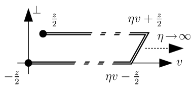
Figure 1: Path of the gauge connection $U$, cf. (4), in the correlator (3).

By allowing for continuous variation of $\eta$, the results obtained in the present work will interpolate continuously and gauge-invariantly between the $\eta=0$ Ji limit and the large $|\eta|$ Jaffe-Manohar limit; note that quark orbital angular momentum is an even function of $\eta$. In the convention adopted below, the $\eta\geq 0$ branch will correspond to a struck quark gradually gathering up torque as it is leaving the proton, owing to final state interactions.

The direction $v$ of the staple is associated with the path of the struck quark in, e.g., a deep-inelastic scattering process; in such a process, the Wilson lines forming the legs of the staple-shaped gauge link represent eikonal approximations of gluon exchanges in the final state. Here, the standard TMD specification ji04 ; aybat ; collbook $v_{T}=0$ will be followed. Since such a hard process is characterized by a large rapidity difference between the struck quark and the initial hadron, a straightforward choice of $v$ which suggests itself would be a light-cone vector. However, this choice leads to severe rapidity divergences rapidrev , which in the factorization framework developed in aybat ; collbook are regulated by taking the staple direction $v$ off the light cone into the spacelike region. The correlator (3) can consequently be characterized in Lorentz-invariant fashion by the additional Collins-Soper type parameter

$$\hat{\zeta}=\frac{v\cdot P}{\sqrt{|v^{2}|}\sqrt{P^{2}}}$$ (5)

in terms of which the light-cone limit is recovered for $\hat{\zeta}\rightarrow\infty$. Note that the specification $v_{T}=0$ implies that the soft factor ${\cal S}[U]$ does not depend on the direction of $z_{T}$, the transverse part of the quark operator separation $z$; one can freely rotate $z_{T}$ in the transverse plane while keeping all other geometric characteristics of the gauge link fixed. In the following, the notation ${\cal S}[U]\equiv{\cal S}(z_{T}^{2})$ will be adopted to emphasize this form of the dependence on $z_{T}$, suppressing dependences on other aspects of the geometry of the gauge link $U$.

An important point to note is that adopting a scheme in which $v$ is chosen to be spacelike is crucial to enable a Lattice QCD evaluation of the proton matrix element in (3). Since Lattice QCD employs a Euclidean time dimension to project out the hadronic ground state, no physical temporal extent can be accomodated in the quark bilocal operator of which one is taking the matrix element. All separations must be purely spatial. Only if $v$ is generically spacelike can one boost the problem to a Lorentz frame in which $v$ becomes purely spatial, and perform the calculation in that frame. Note that, in such a frame, large $\hat{\zeta}$ are realized by large spatial proton momenta ${\bf P}$, cf. (5). Specifically, in the calculations to follow, $v$ will point purely in longitudinal direction, $v\equiv-\vec{e}_{3}$, and, consequently, $\hat{\zeta}=P_{3}/m$, with $m$ denoting the proton mass. Note furthermore that, in the $\eta=0$ limit, the vector $v$ ceases to play an independent physical role as the direction of propagation of the struck quark, and thus $\hat{\zeta}$ ceases to encode a rapidity difference between the proton and the struck quark. Nevertheless, in the specific frame employed for the lattice calculation, one can still use $v\equiv-\vec{e}_{3}$ to construct the parameter $\hat{\zeta}$, which then merely continues to characterize the proton momentum in that frame. Throughout the developments below, $\hat{\zeta}$ will consistently serve to parametrize the approach to the physical limit. Of course, the set of proton momenta which will be accessible in practice in the concrete lattice calculation will be limited; as in lattice TMD calculations tmdlat ; bmlat , extracting information about the large $\hat{\zeta}$ regime presents a challenge in the present calculational framework.

Inserting (2) into (1), one obtains quark orbital angular momentum in terms of the GTMD correlator (3),

$$L^{U}_{3}=-i\int dx\int d^{2}k_{T}\,\epsilon_{ij}k_{T,j}\left.\frac{\partial}{\partial\Delta_{T,i}}\frac{1}{2}\left(W_{++}^{U}(x,\Delta_{T},k_{T})-W_{--}^{U}(x,\Delta_{T},k_{T})\right)\right|_{\Delta_{T}=0}$$ (6)

Note that the GTMD correlator (3) is parametrized by the GTMDs $F_{1i}$, cf. mms ,

$$W_{\Lambda^{\prime}\Lambda}^{U}=\frac{1}{2m}\bar{u}(p^{\prime},\Lambda^{\prime})\left[F_{11}+\frac{i\sigma^{i+}k_{T}^{i}}{P^{+}}F_{12}+\frac{i\sigma^{i+}\Delta_{T}^{i}}{P^{+}}F_{13}+\frac{i\sigma^{ij}k_{T}^{i}\Delta_{T}^{j}}{m^{2}}F_{14}\right]u(p,\Lambda)$$ (7)

Inserted into the particular structure (6), only the $F_{14}$ contribution survives, and one obtains an expression for quark orbital momentum in terms of this GTMD lorce ,

$$L^{U}_{3}=-\int dx\int d^{2}k_{T}\,\left.\frac{k_{T}^{2}}{m^{2}}F_{14}\right|_{\Delta_{T}=0}$$ (8)

Since it is cast purely in terms of momenta, this formulation is best suited for phenomenological applications. The natural setting for a lattice calculation, on the other hand, is not $k$-space, but instead $z$-space, i.e., one calculates directly the proton matrix element in (3). Inserting (3) into (6), quark orbital angular momentum takes the form

$$L^{U}_{3}=\frac{1}{2P^{+}}\epsilon_{ij}\frac{\partial}{\partial z_{T,i}}\frac{\partial}{\partial\Delta_{T,j}}\!\left.\frac{1}{2}\frac{\langle p^{\prime},+|\overline{\psi}(-z/2)\gamma^{+}U\psi(z/2)|p,+\rangle-\langle p^{\prime},-|\overline{\psi}(-z/2)\gamma^{+}U\psi(z/2)|p,-\rangle}{{\cal S}(z_{T}^{2})}\right|_{z^{+}=z^{-}=0\,,\ \Delta_{T}=0\,,\ z_{T}\rightarrow 0}$$ (9)

Thus, in terms of the $z$ and $\Delta$ variables preferred for a Lattice QCD calculation, no Fourier integrals over the generated data are necessary to extract quark orbital angular momentum; this significantly facilitates the numerical analysis. The expression (9) can still be brought into a more compact form. Owing to the symmetric treatment of both the momentum transfer $\Delta_{T}$ and the spin, replacing the proton helicities in (9) by proton spins pointing into the fixed positive and negative $3$-directions, respectively, only generates correction terms in (9) which vanish as $\Delta_{T}\rightarrow 0$. Secondly, the two terms in (9) then yield identical contributions to quark orbital angular momentum, and one can therefore confine oneself to evaluating either one of the two terms. Thus, quark orbital angular momentum can be evaluated more simply as

$$L^{U}_{3}=\frac{1}{2P^{+}}\epsilon_{ij}\frac{\partial}{\partial z_{T,i}}\left.\frac{\partial}{\partial\Delta_{T,j}}\frac{\langle p^{\prime},S^{\prime}=\vec{e}_{3}|\overline{\psi}(-z/2)\gamma^{+}U\psi(z/2)|p,S=\vec{e}_{3}\rangle}{{\cal S}(z_{T}^{2})}\right|_{z^{+}=z^{-}=0\,,\ \Delta_{T}=0\,,\ z_{T}\rightarrow 0}$$ (10)

Note that, formally, one might consider taking the soft factor outside the $z_{T}$-derivative in the limit $z_{T}\rightarrow 0$, since the soft factor depends only on the magnitude of $z_{T}$, not its direction. However, in the presence of a lattice cutoff, the derivative with respect to $z_{T}$ will be realized as a finite difference, and the limit $z_{T}\rightarrow 0$ has to be taken with care. For this reason, the soft factor is left inside the derivative at this stage, deferring a more precise treatment to the practical implementation of (10) in the presence of a lattice cutoff.

III Regularization and renormalization

The form (10) for quark orbital angular momentum is not directly amenable to lattice evaluation, because the soft factor in the Collins factorization scheme aybat ; collbook ; spl2 is not accessible in Lattice QCD; it contains Wilson line structures of varying rapidities, not all of which can be simultaneously boosted to a single instant, a prerequisite for lattice evaluation. As in previous lattice TMD studies tmdlat ; bmlat , this is addressed by forming an appropriate ratio with an additional quantity, such that the soft factors cancel. A convenient choice of such a second quantity can be constructed via the unpolarized TMD $f_{1}(x,k_{T})$. This TMD is obtained from the GTMD $F_{11}$ in the limit of vanishing momentum transfer mms , and thus from the correlator (3) as, cf. the parametrization (7),

$$f_{1}=\left.F_{11}\right|_{\Delta_{T}=0}=\left.W^{U}_{++}\right|_{\Delta_{T}=0}$$ (11)

($W^{U}_{--}$ could likewise be used). On the other hand, integrating $f_{1}$ over all momenta yields the number of valence quarks,

$$n=\int dx\int d^{2}k_{T}\,f_{1}=\frac{1}{2P^{+}}\left.\frac{\langle p^{\prime},S^{\prime}=\vec{e}_{3}|\overline{\psi}(-z/2)\gamma^{+}U\psi(z/2)|p,S=\vec{e}_{3}\rangle}{{\cal S}(z_{T}^{2})}\right|_{z^{+}=z^{-}=0,\Delta_{T}=0,z_{T}\rightarrow 0}$$ (12)

having inserted the explicit form of $W^{U}_{++}$, cf. (3), and also having used that, for $\Delta_{T}=0$, positive helicity corresponds to spin in the $3$-direction. Now, comparing (12) with (10), the two matrix elements contain the same operator, associated accordingly with the same soft factor; one can therefore envisage canceling the soft factors by taking an appropriate ratio. Care has to be taken, however, in defining the $z_{T}\rightarrow 0$ limit. At a finite lattice spacing $a$, distances smaller than $a$ cannot be resolved, and the $z_{T}$-derivative in (10) is realized as a finite difference. It therefore necessarily involves values of the correlator (10) at finite $z_{T}$ for any given finite lattice spacing $a$. Denoting

$$\Phi(z_{T})=\langle p^{\prime},S^{\prime}=\vec{e}_{3}|\overline{\psi}(-z/2)\gamma^{+}U\psi(z/2)|p,S=\vec{e}_{3}\rangle\ ,$$ (13)

(where, for conciseness of notation, all other dependences are being omitted in the argument of $\Phi$), one can specify

$$L^{U}_{3}=\frac{1}{2P^{+}}\epsilon_{ij}\frac{\partial}{\partial\Delta_{T,j}}\frac{1}{2da}\left.\frac{1}{{\cal S}((da)^{2})}\left(\Phi(da\vec{e}_{i})-\Phi(-da\vec{e}_{i})\right)\right|_{z^{+}=z^{-}=0,\Delta_{T}=0}$$ (14)

with a fixed number of lattice spacings $d$, which approximates the derivative as $a\rightarrow 0$. One may contemplate using $d>1$ in order to mitigate lattice artefacts; this will be revisited in the discussion of numerical results below. Note that, since the soft factor does not depend on the direction of $z_{T}$, but only its magnitude, the two terms in the finite difference are associated with an identical soft factor, which can therefore be factored out.

In order to use (12) to form a ratio in which the soft factor cancels, one has to accordingly specify the limit $z_{T}\rightarrow 0$ as

$$n=\frac{1}{2P^{+}}\left.\frac{1}{{\cal S}((da)^{2})}\frac{1}{2}\left(\Phi(da\vec{e}_{i})+\Phi(-da\vec{e}_{i})\right)\right|_{z^{+}=z^{-}=0,\Delta_{T}=0}$$ (15)

which is independent of the transverse direction $\vec{e}_{i}$ used and approximates (12) as $a\rightarrow 0$ in a way which matches the manner in which (14) approximates (10), i.e., using values of $\Phi(z_{T})$ at finite $|z_{T}|=da$ for any given finite lattice spacing $a$. Combining (14) and (15), one obtains the renormalized ratio

$$\frac{L^{U}_{3}}{n}=\frac{1}{da}\epsilon_{ij}\left.\frac{\frac{\partial}{\partial\Delta_{T,j}}\left(\Phi(da\vec{e}_{i})-\Phi(-da\vec{e}_{i})\right)}{\Phi(da\vec{e}_{i})+\Phi(-da\vec{e}_{i})}\right|_{z^{+}=z^{-}=0,\Delta_{T}=0}$$ (16)

(where sums over $i,j$ are still implied), in which the soft factors, and also any multiplicative renormalization constants attached to the quark operators in $\Phi(z_{T})$ have canceled. The ratio (16) is the expression evaluated in practice in the Lattice QCD calculation to be discussed below. Note that also the derivative with respect to $\Delta_{T}$ in practice will have to be approximated by a finite difference. However, contrary to the treatment of the $z_{T}\rightarrow 0$ limit, the $\Delta_{T}\rightarrow 0$ limit is not associated with ultraviolet divergences and is conceptually straightforward, even if it poses numerical challenges, to be discussed further below.

Besides considering the ratio (16) for fixed $d$, such that $|z_{T}|=da\rightarrow 0$ for $a\rightarrow 0$, one can also consider the regime of fixed finite physical distance $|z_{T}|=da$ and define a generalized, $|z_{T}|$-dependent quark orbital angular momentum

$$\frac{L^{U}_{3}}{n}(|z_{T}|)=\frac{1}{|z_{T}|}\epsilon_{ij}\left.\frac{\frac{\partial}{\partial\Delta_{T,j}}\left(\Phi(|z_{T}|\vec{e}_{i})-\Phi(-|z_{T}|\vec{e}_{i})\right)}{\Phi(|z_{T}|\vec{e}_{i})+\Phi(-|z_{T}|\vec{e}_{i})}\right|_{z^{+}=z^{-}=0,\Delta_{T}=0}$$ (17)

in analogy to, e.g., the generalized tensor charge defined in tmdlat . Keeping $|z_{T}|$ finite effectively acts as a regulator on $k_{T}$-integrations such as the ones in (1) and (8).

As the quark operators in $\Phi(z_{T})$, eq. (13), approach each other, i.e., in the limit $z_{T}\rightarrow 0$ once one has set $z^{+}=z^{-}=0$, the correlator becomes singular. In particular, even if one has properly renormalized $\Phi$, at face value, its derivative $\partial\Phi/\partial z_{T,i}$ in general will formally still be divergent at $z_{T}=0$; in $k_{T}$-space, this translates to the observation that, even if one has properly defined the GTMD $F_{14}$, cf. (7),(8), its $k_{T}$-moment (8) still exhibits an ultraviolet divergence. However, at any given resolution scale, differences in $z_{T}$ smaller than that scale are not resolvable, and thus a consistent interpretation of the $z_{T}$-derivative is in terms of a finite difference taken over a distance commensurate with the resolution scale; the aforementioned singularity occurring at arbitrarily small distances is not resolved. As one increases the resolution, probing the ultraviolet behavior more fully, one not only evaluates the $z_{T}$-derivative using smaller distances; one concomitantly evolves $\Phi$ to the higher resolution scale. The combined effect of these adjustments ultimately produces the proper evolution of the orbital angular momentum $L^{U}_{3}$. An explicit observation of this evolution will not be possible in the present work, since calculations were performed only at one fixed lattice spacing $a$; it would be interesting to pursue an evolution study in future work employing data at a sequence of lattice spacings $a$.

In this context, also further remarks regarding the multiplicative nature of the soft factors and the quark field renormalizations, and their consequent cancellation in the ratio (16), are in order. The absorption of divergences into these multiplicative factors is, to begin with, a construction motivated by the continuum theory aybat ; collbook ; spl2 . That it carries over analogously into the lattice formulation is a working assumption which has been discussed in some detail in straightlinks , and was further explored empirically in latt15_by by investigating whether TMD ratios vary under changes of the lattice discretization scheme. Absence of such variations strengthens the hypothesis that the data provide a good representation of the universal continuum behavior within statistical accuracy; conversely, violations of the multiplicative nature of renormalization would presumably manifest themselves in deviations from a universal continuum limit. On the one hand, at finite physical separations $z_{T}$, one would expect that the lattice operators approximate the continuum operators well and inherit their divergence structure; indeed, in latt15_by , results for TMD ratios obtained using differing discretization schemes were consistently found to coincide once $z_{T}$ extends over several lattice spacings. On the other hand, the limit of small $z_{T}$ deserves further scrutiny. As already noted above, the $z_{T}\rightarrow 0$ limit, in particular the $z_{T}$-derivative $\partial\Phi/\partial z_{T,i}$ in that limit, in general contains additional divergences; using different lattice discretization schemes will have an effect analogous to using different combinations of data obtained at varying $d$ to construct the $z_{T}$-derivative, cf. (14). Moreover, mixing between the various composite local operators arising in the $z_{T}\rightarrow 0$ limit can occur, potentially modifying the simple multiplicative renormalization pattern. In the empirical study latt15_by , the stability of TMD ratios under changes of the lattice discretization scheme was generally seen to persist into the small $z_{T}$ regime, indicating that the data continue to represent the universal continuum limit well, with the notable exception of the worm-gear shift $\langle{\bf k}_{x}\rangle^{g_{1T}}$, for which significant deviations between different discretization schemes were observed. The Sivers shift $\langle{\bf k}_{y}\rangle^{\mbox{\scriptsize Sivers}}$, which is the TMD ratio most directly related to the ratio (16) considered here, exhibited no such deviations. Apart from performing an analogous study also directly for the ratio (16), another opportunity to cross-check the behavior of (16) for the need for additional renormalization will ultimately be provided by a comparison of the $\eta=0$ Ji limit with the result for quark orbital angular momentum obtained using Ji’s sum rule, on the same lattice ensemble. It should be noted, however, that the numerical data generated to date will not yet permit definite conclusions in this regard; at the present stage, the aforementioned comparison is affected by significant other systematic uncertainties as well, as discussed further below.

IV Lattice calculation

Numerical data for the present study were generated employing a mixed action scheme in which the valence quarks are realized as domain wall fermions, propagating on a $N_{f}=2+1$ dynamical asqtad quark gauge background. The corresponding gauge ensemble was provided by the MILC Collaboration milc . A fairly high pion mass, $m_{\pi}=518\,\mbox{MeV}$, was used for this exploration in order to reduce statistical fluctuations. Table 1 lists the details of the ensemble.

$L^{3}\times T$	$a$(fm)	$am_{u,d}$	$am_{s}$	$m_{\pi}^{\mbox{\tiny DWF}}$ (MeV)	$m_{N}^{\mbox{\tiny DWF}}$ (GeV)	#conf.	#meas.
$20^{3}\times 64$	0.11849(14)(99)	0.02	0.05	518.4(07)(49)	1.348(09)(13)	486	3888

Table 1: Details of the lattice ensemble. The lattice spacing $a$ was determined using a different scheme, cf. tmdlat , than was employed in LHPC_1 ; LHPC_2 ; as a result, it and the listed hadron masses deviate slightly from the values quoted in the latter references. The uncertainties given for the hadron masses are, in that order, statistical, and stemming from the conversion to physical units via $a$. The values $m_{u,d,s}$ are the bare asqtad quark masses. On each gauge configuration, eight measurements were performed.

The mixed action scheme employed here has been the basis for detailed investigations into hadron structure carried out by the LHP Collaboration LHPC_1 ; LHPC_2 , including the particular ensemble described in Table 1. It was also used in previous lattice TMD studies tmdlat ; bmlat .

Evaluation of the correlator (13), needed to obtain quark orbital angular momentum through (16), proceeds via the calculation of appropriate three-point functions $C_{\mbox{\tiny 3pt}}[\hat{O}]$ as well as two-point functions $C_{\mbox{\tiny 2pt}}$, projected onto a definite proton momentum at the proton sink, as well as a definite momentum transfer at the operator insertion in $C_{\mbox{\tiny 3pt}}[\hat{O}]$,

$$C_{\mbox{\tiny 3pt}}[\hat{O}](t,t_{f},p^{\prime},p) = \sum_{{\bf x}_{f},\,{\bf y}}e^{-i{\bf x}_{f}\cdot{\bf p^{\prime}}+i{\bf y}\cdot({\bf p^{\prime}-p})}\mbox{tr}[\Gamma_{\mbox{\tiny pol}}\langle n(t_{f},{\bf x}_{f})\hat{O}(t,{\bf y})\bar{n}(0,0)\rangle]$$ (18)

$$C_{\mbox{\tiny 2pt}}(t_{f},p^{\prime}) = \sum_{{\bf x}_{f}}e^{-i{\bf x}_{f}\cdot{\bf p^{\prime}}}\mbox{tr}[\Gamma_{\mbox{\tiny pol}}\langle n(t_{f},{\bf x}_{f})\bar{n}(0,0)\rangle]\ ,$$ (19)

constructed using Wuppertal-smeared proton interpolating fields $n(t,{\bf x})$, with the projector $\Gamma_{\mbox{\tiny pol}}=\frac{1}{2}(1+\gamma_{4})\frac{1}{2}(1-i\gamma_{3}\gamma_{5})$ selecting states polarized in the 3-direction. The Euclidean temporal separation between proton sources and sinks was $t_{f}=9a$. The operator $\hat{O}$ is taken to be the operator in (13); as already discussed following eq. (5) further above, the lattice calculation is carried out in a Lorentz frame in which $\hat{O}$ exists at a single time $t$, i.e., the quark operator separation $z$ and the staple direction $v$ are purely spatial. In this frame, $v=-\vec{e}_{3}$ and, consequently, $\hat{\zeta}=P_{3}/m$, cf. (5), in terms of which the physical limit is approached as $\hat{\zeta}$ becomes large. In the present study, only connected diagrams entering $C_{\mbox{\tiny 3pt}}[\hat{O}]$ were calculated. Computationally significantly more expensive disconnected contractions, the magnitudes of which are expected to be minor at the heavy pion mass employed here, are excluded from all numerical results quoted below (they cancel in the isovector $u-d$ quark channel).

To obtain the correlator (13), one forms the three-point to two-point function ratio

$$2E(p^{\prime})\frac{C_{\mbox{\tiny 3pt}}[\hat{O}](t,t_{f},p^{\prime},p)}{C_{\mbox{\tiny 2pt}}(t_{f},p^{\prime})}\longrightarrow\Phi(z_{T})$$ (20)

which exhibits plateaus in $t$ yielding $\Phi(z_{T})$ for $0\ll t\ll t_{f}$. In (20), $E(p^{\prime})=E(p)$ is the energy of the final and of the initial proton state; note that the symmetric treatment of the initial and final momenta $p=P-\Delta_{T}/2$, $p^{\prime}=P+\Delta_{T}/2$ simplifies the ratio required to extract $\Phi(z_{T})$ in (20) compared to the case of general $p,p^{\prime}$ LHPC_1 ; LHPC_2 . In the present exploration, possible excited state contaminations affecting the plateau values determined from (20) at the source-sink separation $t_{f}=9a=1.07\,\mbox{fm}$ were not quantified. They are expected to be small at the heavy pion mass $m_{\pi}=518\,\mbox{MeV}$ considered here; however, it will be necessary to account for them in more quantitative studies at lower pion masses.

In the mixed action calculational scheme employed in the present investigation, HYP-smearing is applied to the gauge configurations before computing the domain wall valence quark propagators. This suppresses dislocations in the fields that could potentially produce spurious mixing between the right-handed and left-handed fermion modes localized on their respective domain walls. These same HYP-smeared gauge fields were also used to assemble the gauge link $U$ in (13). As a consequence, even before cancellation in the ratio (16), renormalization constants and soft factors correspond more closely to their tree-level values.

${\bf P}\cdot aL/(2\pi)$	${\bf\Delta}\cdot aL/(4\pi)$	${\bf z}/a$	$\eta{\bf v}/a$
$(0,0,n_{P})$	$(n_{\Delta},0,0)$	$(0,n_{z},0)$	$(0,0,n_{v})$
$(0,0,n_{P})$	$(0,n_{\Delta},0)$	$(n_{z},0,0)$	$(0,0,n_{v})$

Table 2: Combinations of momenta and gauge link geometries used. The longitudinal momentum index $n_{P}$ took the values $n_{P}=0,1,2$; the transverse momentum transfer index $n_{\Delta}$ took the values $n_{\Delta}=-1,0,1$. Note that the symmetric treatment of the momentum transfer in the initial and final states, $p=P-\Delta_{T}/2$, $p^{\prime}=P+\Delta_{T}/2$, implies that, for the standard periodic spatial boundary conditions used in the present study, the smallest nonzero momentum transfer available is $4\pi/(aL)$. The quark separation index $n_{z}$, corresponding to the width of the staple-shaped gauge link, extended over the integers $n_{z}=-5\ldots 5$; the range of the index $n_{v}$ determining the staple length of the gauge link covered all values for which a numerical signal is discernible (in both the positive and negative directions).

The combinations of gauge link geometries and momenta considered in the calculation are given in Table 2. As far as the gauge link geometries are concerned, the focus of the present investigation is on small values of the quark separation $z_{T}$, and therefore only the restricted range of $n_{z}=-5\ldots 5$ in Table 2 was treated; it is possible to obtain a numerical signal at larger $z_{T}$, cf. the TMD investigations tmdlat ; bmlat . On the other hand, the staple length index $n_{v}$ covered all values for which a numerical signal is discernible. In particular, for $n_{v}=0$, one accesses Ji quark orbital angular momentum, whereas for asymptotically large $n_{v}$, Jaffe-Manohar quark orbital angular momentum is probed. The correlators are time-reversal even, i.e., invariant under reflection of $n_{v}$.

On the other hand, the set of proton momenta accessed in this exploratory investigation is rather limited, both in terms of the longitudinal momentum $P$ as well as the transverse momentum transfer $\Delta_{T}$. This is the source of the most significant systematic uncertainties affecting the results extracted, and thus represents the most severe shortcoming of the data set collected for this study. To extract quark orbital angular momentum, the longitudinal momentum ${\bf P}$ must be extrapolated to large values. The spatial momenta employed in practice, cf. Table 2, have magnitudes $|{\bf P}|=0,0.52,1.04$ GeV and thus remain far from the asymptotic regime. Simultaneously, in terms of the Collins-Soper parameter $\hat{\zeta}$, characterizing the rapidity difference between the vectors $P$ and $v$, these momenta correspond to $\hat{\zeta}=0,0.39,0.78$, respectively; these values likewise are still far from the region in which one would expect to be able to connect to perturbative evolution in $\hat{\zeta}$. To give a tentative indication of the results for quark orbital angular momentum one might expect to obtain at large proton momenta, below, an ad hoc extrapolation will be entertained using the available two nonvanishing values of $|{\bf P}|$. This extrapolation will be guided by the behavior that was observed in a study bmlat of the Boer-Mulders effect in a pion, in which it proved possible to extract the large-$\hat{\zeta}$ limit. However, in order to obtain stringent quantitative results for quark orbital momentum in the proton, it will be necessary to generate data at larger $|{\bf P}|$, and, concomitantly, larger $\hat{\zeta}$ in future work.

Additionally, to extract quark orbital angular momentum, cf. (16), one has to evaluate a derivative of the correlator data with respect to the momentum transfer $\Delta_{T}$ in the forward limit. To obtain an accurate estimate of this derivative, one needs to employ data at small $\Delta_{T}$. However, the nonzero values of the momentum transfer available for this study, cf. Table 2, are quite substantial, $|\Delta_{T}|=1.04$ GeV; note that the symmetric treatment of the momentum transfer in the initial and final states, $p=P-\Delta_{T}/2$, $p^{\prime}=P+\Delta_{T}/2$, implies that, for the standard periodic spatial boundary conditions used in the present study, the smallest nonzero momentum transfer available is $4\pi/(aL)$. In practice, the numerical results presented in the following were extracted by averaging over the finite differences obtained in opposite directions, i.e., using directly the difference between the $n_{\Delta}=\pm 1$ data; the $n_{\Delta}=0$ data served to evaluate the denominator in (16). Using such a finite difference of correlator data at the aforementioned large values of the momentum transfer will lead to a substantial underestimate of the derivative. To obtain a rough idea of the magnitude of the underestimate, note that the combination $F=(\Phi(da\vec{e}_{i})-\Phi(-da\vec{e}_{i}))$ appearing in the numerator of (16), of which one requires the $\Delta_{T}$-derivative, is an odd function of $\Delta_{T}$. Absent more detailed information on the form of its $\Delta_{T}$-dependence, consider modeling it as $F(\Delta_{T})=\Delta_{T}F_{1}(|\Delta_{T}|)$, using the isovector electromagnetic Dirac form factor $F_{1}$ as a proxy for the typical variation of distribution functions with $\Delta_{T}$. The fall-off of $F_{1}$ with $\Delta_{T}$ then gives an indication of the extent to which the numerator of (16) may be underestimated. On the ensemble used in the present study, $F_{1}$ falls off LHPC_2 by (slightly more than) a factor 2 between $\Delta_{T}=0$ and $|\Delta_{T}|=1$ GeV. Thus, a substantial upward correction by a factor of this magnitude must be expected for the extracted values of the quark orbital angular momentum, once this source of systematic bias is eliminated. This is the top priority for future more quantitative studies, and a calculation is currently in preparation which will incorporate a direct method to evaluate the $\Delta_{T}$-derivative exactly rome ; nhasan ; smpriv .

V Numerical results

A critical element in the evaluation of quark orbital angular momentum is a stable extraction of the $z_{T}$-derivative in (10), as realized by the finite difference in (16); a priori, one might expect strongly varying behavior of the correlator $\Phi(z_{T})$, reflecting the singular nature of the $z_{T}\rightarrow 0$ limit. Such behavior could potentially render the evaluation of quark orbital angular momentum via (16) infeasible. Fig. 2 displays results for the ratio (16) as a function of the distance $d$ used to construct the finite difference approximation to the $z_{T}$-derivative, for a fixed Collins-Soper parameter $\hat{\zeta}$ and several fixed staple lengths $\eta|v|$; the derivative with respect to $\Delta_{T}$ was evaluated as a finite difference as discussed in the previous section. The data shown correspond to the isovector $u-d$ quark channel, in which disconnected contributions cancel and the renormalized number of valence quarks is $n=1$, i.e., the ratio (16) is directly a measure of quark orbital angular momentum.

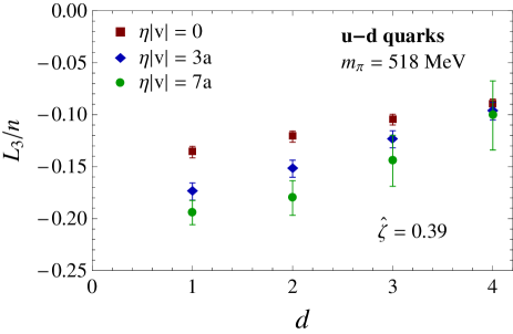
Figure 2: Quark orbital angular momentum in units of the number of valence quarks, as a function of the number of lattice spacings $d$ used to construct the derivative with respect to $z_{T}$ in (14),(16). Data are shown at a fixed $\hat{\zeta}=0.39$ and for three different staple length parameters $\eta$; the isovector $u-d$ quark combination was evaluated. The shown uncertainties are statistical jackknife errors.

The ratio is fairly stable as $d$ is varied, implying an approximately linear behavior of (the $\Delta_{T}$-odd part of) $\Phi(z_{T})$ at small $z_{T}$. In particular, the variation of the ratio data with $d$ tends to decrease as one goes to smaller $d$ and one can assign an approximate value to the $z_{T}$-derivative in (10), as defined by the numerator of (16), employing the data at small values of $d$. It should be noted that, at the finite lattice spacing $a$ employed in the present work, there is no clear separation between, on the one hand, the regime of finite $d$, such that $|z_{T}|=da\rightarrow 0$ as $a\rightarrow 0$, in which the numerator of (16) defines the $z_{T}$-derivative in (10); and, on the other hand, the regime of finite physical $|z_{T}|=da$, in which (16) can be viewed as defining a generalized quark orbital angular momentum, cf. (17). The behavior of the data represents a mixture of the characteristics of the two regimes. As $a\rightarrow 0$, a separation of the regimes will be achieved; the behavior of the data in Fig. 2 suggests that it may be plausible to expect that the ratio (16) will indeed become sharply defined in the finite $d$ regime, i.e., the different discretizations of the $z_{T}$-derivative given by the different values of $d$ converge. On the other hand, in view of Fig. 2 it appears reasonable to suppose that, in the finite $|z_{T}|=da$ regime, the generalized quark orbital angular momentum $(L_{3}/n)(|z_{T}|)$ will exhibit a smooth limit towards the actual quark orbital angular momentum as $z_{T}\rightarrow 0$. It will be useful to explore and test these expectations in future work employing a variety of lattice spacings.

In the discussion to follow, the results obtained at $d=1$ will be used as the best available realization of the $z_{T}$-derivative in (10). Having thus settled on a definite scheme of evaluating both of the derivatives in (10), the remaining parameters on which the results for the quark orbital momentum depend are the staple length $\eta$ and the Collins-Soper parameter $\hat{\zeta}$, where an extrapolation to large $\hat{\zeta}$ must be performed. Note that Fig. 2 provides a first glimpse of the fact that data at different $\eta$ can be clearly distinguished, and that their magnitude is enhanced at nonvanishing $\eta$. This will be studied in detail further below. Before exploring the dependence on the staple length $\eta$, it is useful to examine the $\eta=0$ case, corresponding to Ji quark orbital angular momentum.

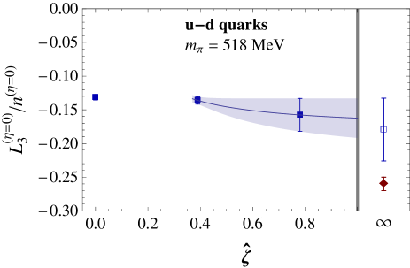
Figure 3: Ji quark orbital angular momentum, i.e., the $\eta=0$ limit, as a function of $\hat{\zeta}$, with an ad hoc extrapolation to infinite $\hat{\zeta}$ (open square). The filled diamond represents the value extracted on the same ensemble via Ji’s sum rule. The isovector $u-d$ quark combination was evaluated. The shown uncertainties are statistical jackknife errors.

Fig. 3 displays the isovector Ji quark orbital angular momentum for all available values of $\hat{\zeta}$, together with an extrapolation to infinite $\hat{\zeta}$ using the fit ansatz $A+B/\hat{\zeta}$. It should be emphasized that this ad hoc ansatz, which will be used repeatedly in the following, is not motivated by any theoretical argument at this point, but has merely been observed to provide a good fit of data in a previous investigation of the Boer-Mulders TMD ratio bmlat , for which an analogous extrapolation in $\hat{\zeta}$ is performed. The extrapolation is thus intended to give simply a heuristic idea of where the $\hat{\zeta}$ limit may plausibly be located. The extrapolated value is confronted with the one obtained on this same lattice ensemble from the standard evaluation of quark orbital angular momentum via Ji’s sum rule LHPC_2 . While the sum rule value lies within two statistical standard deviations of the extrapolated value, a genuine discrepancy between the two is in fact expected, as discussed at the end of the previous section. The replacement of the $\Delta_{T}$-derivative in (16) by a finite difference using a rather large value of $|\Delta_{T}|$ represents a substantial underestimate, possibly by up to a factor of two. The discrepancy seen in Fig. 3 is compatible with this expectation. Indeed, if the extrapolated value in Fig. 3 were to be enhanced by a factor of two, it would overshoot the sum rule value, but still be consistent with it within statistical uncertainty. It thus does not seem implausible to expect that an accurate estimate of the $\Delta_{T}$-derivative in future numerical work will lead to consistent results for Ji quark orbital angular momentum from the present direct evaluation method and the standard sum rule evaluation. In order to roughly cancel the systematic bias stemming from the underestimate of the $\Delta_{T}$-derivative in the discussion of the $\eta\neq 0$ results below, data will be presented relative to the $\eta=0$ Ji value.

The dependence of quark orbital angular momentum on the staple length $\eta$ represents the most interesting feature of the present investigation. As discussed in section II, while the $\eta=0$ case corresponds to Ji quark orbital angular momentum, the $\eta\rightarrow\infty$ limit yields Jaffe-Manohar quark orbital angular momentum, which, contrary to the former, has hitherto not been accessible within Lattice QCD. The difference between the two can be interpreted burk as the integrated torque, due to the final state interactions encoded in the staple-shaped gauge link, accumulated by the struck quark in a deep inelastic scattering process as it is leaving the proton. Since, in the present calculation, the staple length can be varied in small steps, one in fact obtains a quasi-continuous, gauge-invariant interpolation between the Ji and Jaffe-Manohar limits. This is exhibited in Fig. 4, which shows the variation of isovector orbital angular momentum with the staple length parameter $\eta$; the three panels correspond to the three available values of the Collins-Soper parameter $\hat{\zeta}$. In each of the panels, following the change of orbital angular momentum as $\eta$ grows corresponds to observing the struck quark gather up torque on its trajectory leaving the proton, until it reaches the Jaffe-Manohar limit. Note that the data are displayed in units of (the magnitude of) Ji quark orbital angular momentum, obtained at $\eta=0$.

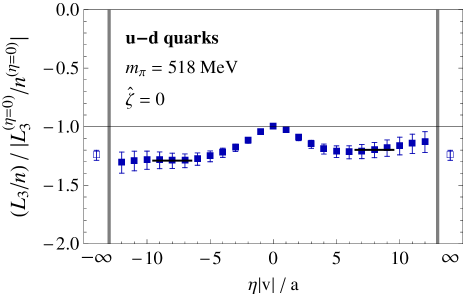
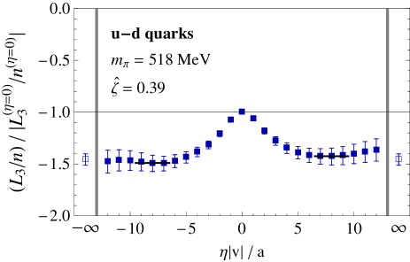
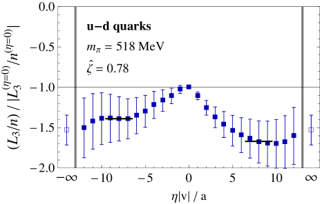
Figure 4: Quark orbital angular momentum as a function of staple length parameter $\eta$, normalized to the magnitude of the $\eta=0$ Ji value. The quark orbital angular momentum is a time-reversal even quantity, i.e., even under $\eta\rightarrow-\eta$. The extrapolated values are obtained by averaging over the $\eta>0$ and $\eta<0$ plateau values, which are each extracted by a fit to the $|\eta||v|/a=7,\ldots,9$ range. The isovector $u-d$ quark combination was evaluated; the three panels display the data for the three available values of $\hat{\zeta}$. The shown uncertainties are statistical jackknife errors.

The effect of the final state interactions seen in the data is substantial. It can be clearly resolved even within the limited statistics employed in the present exploratory calculation, and it enhances quark orbital angular momentum compared with the initial Ji value. As seen in Fig. 4, the effect increases with rising Collins-Soper parameter $\hat{\zeta}$, approaching magnitudes such that the integrated torque accumulated in reaching the Jaffe-Manohar limit amounts to as much as roughly half of the initial Ji orbital angular momentum carried by the quark. The increasing behavior with $\hat{\zeta}$ also implies that the effect is likely to survive extrapolation to the $\hat{\zeta}\rightarrow\infty$ limit. A corresponding extrapolation, again employing the fit ansatz $A+B/\hat{\zeta}$, is exhibited in Fig. 5. Shown are data for the integrated torque

$$\tau_{3}=\frac{L^{(\eta=\infty)}_{3}}{n^{(\eta=\infty)}}-\frac{L^{(\eta=0)}_{3}}{n^{(\eta=0)}}\ ,$$ (21)

i.e., the difference between Jaffe-Manohar and Ji quark orbital momentum, in units of the magnitude of Ji quark orbital momentum. A signal is indeed obtained in the $\hat{\zeta}\rightarrow\infty$ limit. Note that the integrated torque $\tau_{3}$ corresponds to a Qiu-Sterman type correlator burk ; eomlir . The calculation of $\tau_{3}$ presented here amounts to an evaluation of that genuine twist-three term.

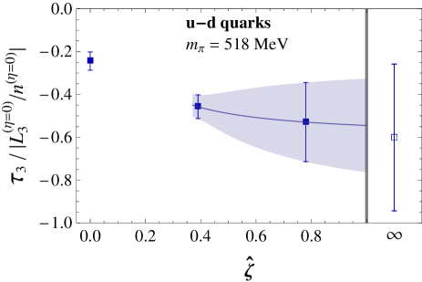
Figure 5: Torque accumulated by the struck quark in a deep inelastic scattering process, cf. main text, normalized to the magnitude of the $\eta=0$ Ji orbital angular momentum, as a function of $\hat{\zeta}$, with an ad hoc extrapolation to infinite $\hat{\zeta}$. The isovector $u-d$ quark combination was evaluated. The shown uncertainties are statistical jackknife errors.

All data presented above concern the isovector $u-d$ quark combination, in which disconnected diagrams cancel. Of interest is also the decomposition by flavor, shown in Figs. 6 and 7. In these flavor-decomposed data, disconnected contributions are omitted; they are, however, expected to be minor at the heavy pion mass used for the present calculation. Fig. 6 exhibits quark orbital angular momentum as a function of staple length parameter $\eta$, for a fixed value of the Collins-Soper parameter $\hat{\zeta}$, analogous to Fig. 4. Displayed are data for the $d$ quark and for the two $u$ quarks, i.e., $L_{3}^{U}/n$ for $u$ quarks has been multiplied by 2 to compensate for $n=2$ in the $u$ quark case. Displayed furthermore is the total (isoscalar) quark orbital angular momentum, which was obtained here simply by adding the aforementioned “$d$” and “$2u$” contributions (at finite statistics, this may differ slightly from evaluating instead $3L_{3,u+d}/n_{u+d}$). The data are again given in units of the magnitude of the isovector Ji quark orbital angular momentum, i.e., in Fig. 6 at $\eta=0$, the difference between the “$2u$” and “$d$” data is unity.

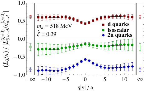
Figure 6: Flavor-separated orbital angular momentum as a function of staple length parameter $\eta$, analogous to Fig. 4, at fixed $\hat{\zeta}=0.39$. Shown are data for $d$ quarks, for two $u$ quarks (i.e., the $u$-quark data for $L_{3}^{U}/n$ have been multiplied by $2$ to compensate for $n=2$ in the $u$-quark case), and the isoscalar total quark orbital angular momentum. The latter was obtained by adding the “$d$” and “$2u$” data. All data are still normalized by the magnitude of $u-d$ Ji orbital angular momentum, i.e., at $\eta=0$, the “$2u$” and “$d$” data differ by unity. The shown uncertainties are statistical jackknife errors.

The flavor-separated data in Fig. 6 reproduce the well-known cancellation between the $d$- and $u$-quark orbital angular momenta in the proton LHPC_1 ; LHPC_2 , which combine to yield only a small negative residual contribution to the spin of the proton at the pion mass used in the present study. This property persists as one departs from Ji quark orbital momentum and adds torque to arrive at Jaffe-Manohar quark orbital momentum. Fig. 7 displays results for the integrated torque, cf. (21), in analogy to Fig. 5, including extrapolations of the data at different Collins-Soper parameters $\hat{\zeta}$ to the $\hat{\zeta}\rightarrow\infty$ limit. The results at $\hat{\zeta}=0.78$ exhibit fairly large statistical fluctuations, which may be the source of the seemingly uncharacteristic behavior of the $d$-quark data point. It would be natural to expect monotonous behavior as a function of $\hat{\zeta}$, and the aforementioned data point may thus well represent a downward fluctuation; it leads to an extrapolated $d$-quark torque compatible with zero, driving the isoscalar combination to negative values (albeit with a large statistical uncertainty). Another, more physical, reason to suspect a spurious downward fluctuation in this case is that final state interaction effects on quark transverse momenta in the proton generally tend to be stronger for a $d$-quark than a (single) $u$-quark, as embodied, e.g., in the Sivers shift or the Boer-Mulders shift tmdlat ; bmlat This suggests that a subtle interplay between transverse positions and momenta of the quarks would be needed to generate a deviating pattern for the integrated torque. Indeed, the substantial statistical uncertainties at $\hat{\zeta}=0.78$ do in fact still render the data compatible with a $d$-quark integrated torque that is stronger than a (single) $u$-quark integrated torque. A higher statistics calculation is needed to draw definite conclusions on this point. At present, in view of the sizeable uncertainties, the extrapolated results are nevertheless compatible with the conclusions drawn above from Fig. 6 at the fixed value $\hat{\zeta}=0.39$.

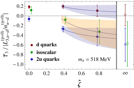
Figure 7: Flavor-separated torque accumulated by the struck quark in a deep inelastic scattering process, as a function of $\hat{\zeta}$, analogous to Fig. 5, with ad hoc extrapolations to infinite $\hat{\zeta}$. Shown are data for $d$ quarks, for two $u$ quarks (i.e., the $u$-quark data for $\tau_{3}$ have been multiplied by $2$ to compensate for $n=2$ in the $u$-quark case), and the isoscalar combination. The latter was obtained by adding the “$d$” and “$2u$” data. All data are still normalized by the magnitude of $u-d$ Ji orbital angular momentum. Isoscalar data are slightly displaced horizontally for better visibility. The shown uncertainties are statistical jackknife errors.

VI Conclusions and outlook

The present exploration demonstrates the feasibility of calculating the quark orbital angular momentum in a proton in Lattice QCD directly, using a Wigner distribution-based approach. Given a Wigner distribution of quark parton positions and momenta in the transverse plane with respect to proton motion, one can directly evaluate their average cross product, i.e., longitudinal orbital angular momentum. The Wigner distribution in question can be derived from appropriate proton matrix elements lorce . As is familiar from the definition of transverse momentum-dependent parton distributions (TMDs), transverse momentum information can be extracted by employing a quark bilocal operator; the transverse quark separation in this operator is Fourier conjugate to the quark transverse momentum. On the other hand, by generalizing the TMD matrix element to non-zero momentum transfer, the TMD information is supplemented with impact parameter information. One thus arrives at generalized transverse momentum-dependent parton distributions (GTMDs) mms , which, appropriately Fourier-transformed, yield the desired Wigner distribution. In view of this construction, many of the concepts and techniques employed in lattice TMD studies tmdlat ; bmlat can be brought to bear on the direct evaluation of quark orbital angular momentum in a proton.

In order to define a gauge-invariant observable, the bilocal TMD operator must contain a gauge connection between the quarks. Different choices of the path along which the connection is evaluated encode different definitions of quark orbital angular momentum jist ; hatta ; burk , including the Ji and Jaffe-Manohar definitions. The approach developed here has thus opened the possibility of going beyond the lattice studies of quark orbital angular momentum carried out to date, which were limited to calculating specifically Ji orbital angular momentum via Ji’s sum rule. Indeed, the present investigation has provided a quasi-continuous, gauge-invariant interpolation between Ji and Jaffe-Manohar orbital angular momentum, by deforming the gauge connection path in small steps. The difference between the two definitions is given by Burkardt’s torque burk , i.e., the integrated torque accumulated by the struck quark in a deep inelastic scattering process as it is leaving the proton; it corresponds to a genuine twist-three, Qiu-Sterman type correlator. The aforementioned interpolation allows one to directly follow the gradual accumulation of this torque along the quark’s path.

The gauge connection contained in the bilocal TMD operator is associated with ultraviolet divergences which, in the continuum Collins factorization scheme aybat ; collbook ; spl2 , are absorbed into multiplicative soft factors appearing alongside the renormalization factors associated with the quark fields. As in lattice TMD studies, also in the present context an appropriate ratio can be formed in which these factors cancel; it is assumed that their multiplicative nature carries over into the lattice formulation. The renormalized quantity evaluated in effect is $L_{3}/n$, the longitudinal quark orbital angular momentum component in units of the number of valence quarks, for the quark flavor under consideration. Accessing this quantity entails, in particular, evaluating the derivative of the relevant proton matrix element with respect to the quark separation $z_{T}$ in the employed quark bilocal operator, in the limit of vanishing $z_{T}$. This limit must be taken with care owing to the associated ultraviolet singularities. The behavior of the gathered data with varying $z_{T}$ was considered in particular, revealing a fairly stable behavior that suggests that the aforementioned $z_{T}$-derivative can be extracted unambiguously in the continuum limit. This is a prerequisite for the application of the method.

The principal new physical insight gleaned from the present exploration concerns the behavior of Jaffe-Manohar quark orbital angular momentum relative to its Ji counterpart. Their difference, Burkardt’s torque, is clearly resolvable in the data and is sizeable, amounting to roughly one half of Ji quark orbital angular momentum. The torque enhances Jaffe-Manohar quark orbital angular momentum relative to Ji quark orbital angular momentum. As already noted above, the data gathered within this investigation provide a quasi-continuous, gauge-invariant interpolation between the two limits.

The most significant shortcoming of the data set obtained in the present exploration is the limited set of proton momenta, both in the longitudinal and the transverse directions. In particular, only one fairly large value of the momentum transfer $\Delta_{T}$ in the transverse plane is available, and the $\Delta_{T}$-derivative necessary to extract orbital angular momentum is substantially underestimated by the finite difference obtained using the aforementioned $\Delta_{T}$ value. Thus, while the above conclusions concerning the relative comparison between Jaffe-Manohar and Ji quark orbital angular momentum are presumably robust with respect to this systematic bias, in absolute terms, the results extracted systematically underestimate the quark orbital angular momentum present in the proton. This, indeed, is manifested clearly in the case of Ji orbital angular momentum, through the comparison with the corresponding indirect Ji sum rule lattice evaluation on the same ensemble. Removing this systematic bias is foremost on the agenda for future work. A calculation is in preparation which will incorporate a direct method to evaluate the $\Delta_{T}$-derivative exactly rome ; nhasan ; smpriv , related to twisted boundary conditions on the quark fields. The aforementioned comparison with the standard evaluation of Ji orbital angular momentum via Ji’s sum rule will provide a valuable benchmark for the removal of systematic bias.

Moreover, the data are to be extrapolated to large Collins-Soper parameter $\hat{\zeta}$, realized in the employed Lorentz frame via large proton momenta. Although the availability of several longitudinal proton momenta in the gathered data set allowed for an ad hoc estimation of the large-$\hat{\zeta}$ limit, calculations at larger proton momenta are clearly desirable. In this respect, the improved proton sources explored in highmom ; sspriv provide a perspective for generating data that permit a more quantitative treatment of the large-$\hat{\zeta}$ limit.

Further topics for future exploration include the investigation of varying lattice spacing $a$, with a view towards studying, in particular, the $a\rightarrow 0$ behavior of the $z_{T}$-derivative discussed above, as well as observing the evolution of the extracted quark orbital angular momentum. Also, efforts to approach the physical pion mass in these calculations must be undertaken. On a more theoretical level, a decomposition of the proton matrix element under consideration into Lorentz-invariant amplitudes, analogous to the one employed in lattice TMD studies tmdlat ought to provide valuable further insight into the systematics of the data and aid in the extrapolation to large $\hat{\zeta}$, cf. the study of the Boer-Mulders TMD ratio bmlat .

References

- (1) J. Ashman et al. [European Muon Collaboration], Phys. Lett. B206, 364 (1988).
- (2) J. Ashman et al. [European Muon Collaboration], Nucl. Phys. B328, 1 (1989).
- (3) E. Leader and C. Lorcé, Phys. Rept. 541, 163 (2014).
- (4) K.-F. Liu and C. Lorcé, Eur. Phys. J. A 52, 160 (2016).
- (5) X. Ji, Phys. Rev. Lett. 78, 610 (1997).
- (6) R. Jaffe and A. Manohar, Nucl. Phys. B337, 509 (1990).
- (7) Y. Hatta, Phys. Lett. B708, 186 (2012).
- (8) N. Mathur, S. J. Dong, K. F. Liu, L. Mankiewicz and N. C. Mukhopadhyay, Phys. Rev. D 62, 114504 (2000).
- (9) M. Deka, T. Doi, Y.-B. Yang, B. Chakraborty, S. J. Dong, T. Draper, M. Glatzmaier, M. Gong, H.-W. Lin, K.-F. Liu, D. Mankame, N. Mathur and T. Streuer, Phys. Rev. D 91 (2015), 014505 (2015).
- (10) M. Göckeler, R. Horsley, D. Pleiter, P. E. L. Rakow, A. Schäfer, G. Schierholz and W. Schroers [QCDSF Collaboration], Phys. Rev. Lett. 92, 042002 (2004).
- (11) A. Sternbeck, M. Göckeler, P. Hägler, R. Horsley, Y. Nakamura, A. Nobile, D. Pleiter, P. E. L. Rakow, A. Schäfer, G. Schierholz and J. Zanotti, PoS LATTICE2011, 177 (2011).
- (12) G. Bali, S. Collins, M. Göckeler, R. Rödl, A. Schäfer and A. Sternbeck, PoS LATTICE2015, 118 (2016).
- (13) C. Alexandrou, J. Carbonell, M. Constantinou, P. A. Harraud, P. Guichon, K. Jansen, C. Kallidonis, T. Korzec and M. Papinutto, Phys. Rev. D 83, 114513 (2011).
- (14) C. Alexandrou, M. Constantinou, S. Dinter, V. Drach, K. Jansen, C. Kallidonis and G. Koutsou, Phys. Rev. D 88, 014509 (2013).
- (15) P. Hägler et al. [LHP Collaboration], Phys. Rev. D 77, 094502 (2008).
- (16) J. D. Bratt et al. [LHP Collaboration], Phys. Rev. D 82, 094502 (2010).
- (17) S. Syritsyn, J. Green, J. Negele, A. Pochinsky, M. Engelhardt, P. Hägler, B. Musch and W. Schroers, PoS LATTICE2011, 178 (2011).
- (18) Y. Zhao, K.-F. Liu and Y. Yang, Phys. Rev. D93 054006 (2016).
- (19) A. Courtoy, G. Goldstein, J. Gonzalez Hernandez, S. Liuti and A. Rajan, Phys. Lett. B731, 141 (2014).
- (20) S. Meißner, A. Metz and M. Schlegel, JHEP 0908, 056 (2009).
- (21) P. Hägler, B. U. Musch, J. W. Negele and A. Schäfer, Europhys. Lett. 88, 61001 (2009).
- (22) B. U. Musch, P. Hägler, J. W. Negele and A. Schäfer, Phys. Rev. D 83, 094507 (2011).
- (23) B. Musch, P. Hägler, M. Engelhardt, J. Negele and A. Schäfer, Phys. Rev. D 85, 094510 (2012).
- (24) M. Engelhardt, P. Hägler, B. Musch, J. Negele and A. Schäfer, Phys. Rev. D 93, 054501 (2016).
- (25) C. Lorcé and B. Pasquini, Phys. Rev. D 84, 014015 (2011).
- (26) D. Boer, M. Diehl, R. Milner, R. Venugopalan, W. Vogelsang, D. Kaplan, H. Montgomery, S. Vigdor et al., arXiv:1108.1713.
- (27) J. C. Collins, Foundations of Perturbative QCD (Cambridge University Press, 2011).
- (28) M. Echevarria, A. Idilbi, K. Kanazawa, C. Lorcé, A. Metz, B. Pasquini and M. Schlegel, Phys. Lett. B759, 336 (2016).
- (29) M. Burkardt, Phys. Rev. D 88, 014014 (2013).
- (30) X. Ji, X. Xiong and F. Yuan, Phys. Rev. Lett. 109, 152005 (2012).
- (31) A. Rajan, A. Courtoy, M. Engelhardt and S. Liuti, Phys. Rev. D 94, 034041 (2016).
- (32) X. Ji, J.-P. Ma and F. Yuan, Phys. Rev. D 71, 034005 (2005).
- (33) S. M. Aybat and T. Rogers, Phys. Rev. D 83, 114042 (2011).
- (34) J. C. Collins, T. C. Rogers and A. M. Stasto, Phys. Rev. D 77, 085009 (2008).
- (35) S. M. Aybat, J. C. Collins, J.-W. Qiu and T. C. Rogers, Phys. Rev. D 85, 034043 (2012).
- (36) B. Yoon, T. Bhattacharya, M. Engelhardt, J. Green, R. Gupta, P. Hägler, B. Musch, J. Negele, A. Pochinsky and S. Syritsyn, PoS LATTICE2015, 116 (2016).
- (37) C. Aubin, C. Bernard, C. DeTar, J. Osborn, S. Gottlieb, E. Gregory, D. Toussaint, U. Heller, J. Hetrick and R. Sugar, Phys. Rev. D 70, 094505 (2004).
- (38) G. M. de Divitiis, R. Petronzio and N. Tantalo, Phys. Lett. B718, 589 (2012).
- (39) N. Hasan, M. Engelhardt, J. Green, S. Krieg, S. Meinel, J. Negele, A. Pochinsky and S. Syritsyn, PoS LATTICE2016, 147 (2017).
- (40) S. Meinel, private communication.
- (41) G. Bali, B. Lang, B. Musch and A. Schäfer, Phys. Rev. D 93, 094515 (2016).
- (42) S. Syritsyn, private communication.
- (43) R. G. Edwards and B. Joó [SciDAC Collaboration], Nucl. Phys. Proc. Suppl. 140, 832 (2005).