Numerical study of parametric pumping current in mesoscopic systems in the presence of magnetic field

Abstract

We numerically study the parametric pumped current when magnetic field is applied both in the adiabatic and non-adiabatic regimes. In particular, we investigate the nature of pumped current for systems with resonance as well as anti-resonance. It is found that in the adiabatic regime, the pumped current changes sign across the sharp resonance with long lifetime while the non-adiabatic pumped current at finite frequency does not. When the lifetime of resonant level is short, the behaviors of adiabatic and non-adiabatic pumped current are similar with sign changes. Our results show that at the energy where complete transmission occurs the adiabatic pumped current is zero while non-adiabatic pumped current is non-zero. Different from the resonant case, both adiabatic and non-adiabatic pumped current are zero at anti-resonance with complete reflection. We also investigate the pumped current when the other system parameters such as magnetic field, pumped frequency, and pumping potentials. Interesting behaviors are revealed. Finally, we study the symmetry relation of pumped current for several systems with different spatial symmetry upon reversal of magnetic field. Different from the previous theoretical prediction, we find that a system with general inversion symmetry can pump out a finite current in the adiabatic regime. At small magnetic field, the pumped current has an approximate relation $I(B)\approx I(-B)$ both in adiabatic and non-adiabatic regimes.

I introduction

The idea of parametric electron pump was first addressed by Thoulessthouless , which is a mechanism that at zero bias a dc current is pumped out by periodically varying two or more system parameters. Over the years, there has been intensive research interest concentrated on parametric electron pump.thouless1 ; niu ; nazarov ; shutenko ; chu Electron pump has been realized on quantum dot setupaleiner1 consisting of AlGaAs/GaAs heterojunctionswitkes . Low dimensional nanostructures, such as carbon nanotubes (CNT)ydwei2 ; levitov and graphenegraphene1 ; graphene2 were also proposed as potential candidates. Investigation on electron pump also triggers the proposal of spin pumpwatson ; benjamin ; chao , in which a spin current is induced by various means.

At low pumping frequency limit, the variation of the system is relatively slow than the process of energy relaxationswitkes1 . Hence the system is nearly in equilibrium and we could deal with the adiabatic pump by equilibrium methods. On the other hand, non-adiabatic pump refers to the case that pumping process is operated at a finite frequency. In the non-adiabatic regime, non-equilibrium transport theory should be employed. Theoretical methods adopted in the research field includes conventional scattering matrix theorybrouwer1 ; brouwer2 ; andreev , Floquet scattering matrixkim1 ; buttiker1 and non-equilibrium Green’s function (NEGF) methodbaigeng1 ; baigeng2 , as well as other methodologies to both adiabatic aharony and non-adiabaticsen electron pumps.

The electron pump is a phase coherent phenomenon, since the cyclic variation of system parameters affects the phase of wave function with respect to its initial valuezhou . As a result, it is very sensitive to the external magnetic field. In the experimental work of Switkes et.alswitkes , at adiabatic limit, the pumped current of a open quantum dot system with certain spatial symmetry is showed invariant upon reversal magnetic field. The conclusion was confirmed by theoretical works using Floquet scattering matrix methodaleiner2 ; kim ; buttiker2 . Later it was numerically suggestedcsli that the pumped spin current also has certain spatial symmetries.

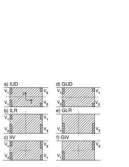
Figure 1: Sketch of the spatial reflection symmetries: (a) instantaneous up-down (IUD); (b) instantaneous left-right (ILR); (c)instantaneous inversion (IIV); (d) general up-down (GUD); (e) general left-right (GLR); (f) general inversion (GIV). Shadow rectangular indicates for the pumping region and dark gray blocks stand for potential barriers defining the spatial symmetry of the system. The pumping potentials are right on top of these confining potentials.

In this paper, we aim to numerically investigate the pumped current in the presence of magnetic field. Both adiabatic and non-adiabatic pumped current are calculated. We focus on the nature of pumped current for the mesoscopic systems with resonance with complete transmission and anti-resonance with complete reflection. We find that the behaviors of adiabatic and non-adiabatic pumped current are very different. In the non-adiabatic regime, the pumped current is nonzero at resonance while it is zero at anti-resonance. However, the adiabatic pumped current is always zero regardless of types of resonance. Since there is no external driving force, the direction of current depend only on the system parameters. Our numerical results show that the adiabatic pumped current reverses it sign at the resonance or anti-resonance. For non-adiabatic pumped current, the sign reversal depends on the lifetime of the resonant states. The non-adiabatic pumped current change the sign near the resonant point only when the lifetime is short. We also study the pumped current as a function of magnetic field. We find that as the system enters the quantum Hall regime with increasing magnetic field strength, the pumping current vanishes. Since in quantum Hall regime electron wave function appears as edge state, it will circumvent the confining potentials shown in Fig.1. Pumping potentials overlapping in space with confining potentials present no modulation on the electron wave function during the variation period. Hence there is zero pumped current in the Quantum Hall regime. We also examine the pumped current and its relation with other system parameters such as pumping frequency and pumping potential amplitude. Finally we also investigate the symmetry properties of the pumped electron current of systems with certain spatial symmetry in the presence of magnetic field by the Green’s function method. Six spatial symmetries studied in Ref.kim are considered, both at the adiabatic and non-adiabatic cases, which are instantaneous up-down (IUD), left-right (ILR), and inversion symmetries (IIV) and the corresponding non-instantaneous/general up-down (GUD), left-right (GLR), and inversion symmetries (GIV), respectively (see Fig.1). The electron pump is driven by periodical modulation of potentials which share the same spatial coordinates with the confining potentials which preserve reflection symmetry of the system. Most of our numerical results agree with the conclusions from Floquet scattering theoryaleiner2 ; kim , except for the general inversion symmetry (GIV) ( setup $f$ in Fig.1 ). In contrast with the theoretical prediction that the adiabatic pumped current $I^{ad}\approx 0$ for this spatial symmetry, our numerical calculation shows that the pumped current is finite and further investigation reveals that there is an approximate symmetry relation of the current as setup $e$ at small magnetic field, which is the experimental setupswitkes . The conclusion suggests that the general left-right (GLR) spatial symmetry has a rather strong impact on the pumped current, which leads to the quite accurate relation $I(B)=I(-B)$ in the experimental finding. The result also holds for the non-adiabatic case.

Our paper is organized as follows. In the next section we will describe the numerical method first followed by the numerical results and discussions in section III. Finally, conclusion is given in section IV.

II theoretical formalism and methodology

We consider a quantum dot system consisting of a coherent scattering region and two ideal leads which connect the dot to electron reservoirs. The whole system is placed in x-y plane and a magnetic field is applied. The single electron Hamiltonian of the scattering region is simply

$$H=\frac{(\textbf{p}+e\textbf{A}/c)^{2}}{2m^{*}}+V(x,y,t)$$

where A is the vector potential of the magnetic field. Here the magnetic field is chosen to be along z-direction with B=(0, 0, B). The vector potential has only x-component in the Landau gauge , A=(-By, 0, 0).

$$H=H_{0}+V_{p}$$

where

$$H_{0}=(-i\hbar\frac{\partial}{\partial x}-\frac{e}{c}By)^{2}+(-i\hbar\frac{\partial}{\partial y})^{2}+V_{0}(x,y)$$

and $V_{p}$ is a time-dependent pumping potential given by $V_{p}(x,y,t)=\sum_{j}V_{j}(x,y)\cos(\omega t+\phi_{j})$.

For the adiabatic electron pump, the average current flowing through lead $\alpha$ due to the slow variation of system parameter $V_{j}$ in one period is given bybrouwer1

$$I_{\alpha} = \frac{1}{\tau}\int_{0}^{\tau}dt\frac{dQ_{\alpha}(t)}{dt}$$ (1)

$$= \frac{q\omega}{2\pi}\int_{0}^{\tau}dt\sum_{j}\frac{dN_{\alpha}}{dV_{j}}\frac{dV_{j}}{dt}$$

where $\tau=2\pi/\omega$ is the variation period of parameter $V_{j}$ and $\omega$ the corresponding frequency. For simplicity we take $\omega=1$ in the adiabatic case. $\alpha$= L or R labels the lead. The so-called emissivity $dN_{\alpha}/dV_{j}$ is conventionally defined in terms of the scattering matrix $S_{\alpha\beta}$ asbrouwer1 ; ydwei1

$$\frac{dN_{\alpha}}{dV_{j}}=\int\frac{dE}{2\pi}(-\partial_{E}f)\sum_{\beta}\text{Im}\frac{\partial S_{\alpha\beta}}{\partial V_{j}}S_{\alpha\beta}^{\ast}$$ (2)

In the language of Green’s function, the above equation is equivalent to the following formbaigeng2

$$I_{\alpha}=q\int_{0}^{\tau}dt\int\frac{dE}{2\pi}(-\partial_{E}f)\text{Tr}\left[\Gamma_{\alpha}G^{r}\frac{dV_{p}}{dt}G^{a}\right]$$ (3)

where the instantaneous retarded Green’s function $G^{r}$ in real space is defined as

$$G^{r}(E,t)=(E-H(t)-\Sigma^{r})^{-1}$$ (4)

where $\Sigma^{r}$ is the self-energy due to the leads.

Whereas for non-adiabatic pump at finite frequency, the pumped current up to the second order in pumping potential is derived as baigeng1

$$I_{\alpha}=-iq\sum_{jk=1,2}\int\frac{dE}{8\pi}\text{Tr}[\Gamma_{\alpha}G^{r}_{0}V_{j}((f-f_{-})(G^{r-}_{0}-$$

$$G^{a-}_{0})e^{i\phi_{kj}}+(f-f_{+})(G^{r+}_{0}-G^{a+}_{0})e^{-i\phi_{kj}})V_{k}G^{a}_{0}]$$ (5)

where $\Gamma_{\alpha}$ is the linewidth function of lead $\alpha$ defined as $\Gamma_{\alpha}=i[\Sigma_{\alpha}^{r}-\Sigma_{\alpha}^{a}]$; $f=f(E)$ and $f_{\pm}=f(E\pm\omega)$ are the Fermi distribution functions; $\phi_{kj}=\varphi_{j}-\varphi_{k}$ is the phase difference between the two pumping potentials. Here $G^{0r}=G^{0r}(E)$ and $G^{0r\pm}=G^{0r\pm}(E\pm\omega)$ are the retarded Green’s functions where there is no pumping potentials. In the following section, we will use Eqs. (3) and (5) to carry on numerical investigations and all the numerical work are done at the zero temperature. In the calculation we consider a square quantum dot with size $0.7\mu m\times 0.7\mu m$, of the same order as in the experimental setup.switkes Two open leads with the same width connect the dot to the electron reservoirs. The quantum dot is then discretized into a $40\times 40$ mesh. Hopping energy $t=\hbar^{2}/2m^{*}a^{2}$ sets the energy scale with $a$ the lattice spacing and $m^{*}$ the effective mass of electrons in the quantum dot. Dimensions of other relevant quantities are then fixed with respect to $t$.

III numerical results and discussion

In this section, numerical results will be presented. To test our numerical method, we first study the reflection symmetry of pumped current on inverse of magnetic field. Other properties of the current will be discussed in the second sub-section.

To check the symmetry of the pumped current we assume $V_{0}=\sum_{j=1,2}V_{j}(x,y)$ in our numerical calculation. In Fig.1, we have schematically plotted 6 setups with different spatial symmetries of interest. In setups $a,b$, and $c$, the spatial symmetries are kept at any moment during the pumping period. Hence we label them instantaneous up-down (IUD), instantaneous left-right (ILR), and instantaneous inversion (IIV) symmetries, respectively. On the other hand, symmetries are broken during the whole pumping cycle except when $\phi_{jk}=n\pi$ in setup $d,e$, and $f$. They are correspondingly labeled as general up-down (GUD), general left-right (GLR), and general inversion (GIV) symmetries. All potential profiles locate at the boundary of the pumping region, i.e., the first and/or last layer in the discrete lattice (see the dark gray region).

III.1 Symmetry of pumped current

Before the presenting numerical results, we would like to point out that for setup $c$ with instantaneous inversion symmetry (IIV), the theoretical predictions aleiner2 ; kim and our numerical calculations give the same result: the pumped current is exact zero at both adiabatic and non-adiabatic cases that is independent of $B$ and $\phi_{12}$. The phenomena can be straightforwardly understood by Floquet scattering matrix theorykim . In IIV setup, it is obvious that the transmission coefficient of an electron traveling from the left lead to the right $T_{R\leftarrow L}$ is always equal to that of an electron moving in the opposite direction, $T_{L\leftarrow R}$, i.e.,

$$T_{R\leftarrow L}=T_{L\leftarrow R}$$

From the Landauer-Büttiker formula, the electric current along the left to right region is given by

$$I_{R\leftarrow L}=\frac{2e}{h}\int dET_{R\leftarrow L}(E)f(E)$$

while $I_{L\leftarrow R}$ is defined in a similar way. Then the pumped current through the left lead is defined asbuttiker2 ; kim

$$I_{L}=I_{L\rightarrow R}-I_{R\rightarrow L}=0$$ (6)

The conclusion holds for any particular moment, which means that there will be no pumped current at all. Hence in the following we will not discuss the case of setup $c$.

First we examine the relation between the adiabatically pumped current $I^{ad}$ and phase difference $\phi_{12}$ of the pumping potentials calculated from Eq.(3). A sinusoidal behavior is observed at a relatively small pumping amplitude $V_{p}$=0.5 for all setups in Fig.1. The sinusoidal form of $I^{ad}(\phi_{12})$ represents a generic property of adiabatic electron pump at small $V_{p}$. Driven by the cyclic variation of two time-dependent system parameters, the pumped current is directly related to the area enclosed by the parameters in parametric space. At small pumping amplitudes, the leading order of $I^{ad}$ is proportional to the phase difference between the pumping potentials, $I^{ad}\propto V_{p}\sin\phi_{12}$ brouwer1 . However, the relation doesn’t hold for large pumping amplitude. To demonstrate this we have calculated current pumping through the setup with symmetry ILR at a large potential $V_{p}$=1.6. As shown in Fig.2 the sinusoidal relation is clearly destroyed. Except for this difference arising from the pumping amplitude $V_{p}$, there is a general antisymmetry relation between the pumped current and the phase difference $\phi_{12}$ for all setups: $I(\phi_{12})=-I(-\phi_{12})$. Naturally, $I(\phi_{12}=n\pi)=0$. This is understandable since two simultaneously varying parameters enclose a line rather than an area in the parametric space, the pumped current vanishes. This result, however, does not hold for non-adiabatic case where the frequency gives additional dimension of parametric space. Another result of interest is that, in contrast to the theoretical prediction $I^{ad}\approx 0$ for the setup of GIV symmetry kim , the pumped current from the setup of GIV is finite and has the same order of magnitude as that of GLR symmetry.

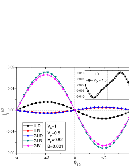
Figure 2: The adiabatically pumped current as a function of phase difference $\phi_{12}$ for different spatial symmetries of the pumping system at pumping amplitude $V_{p}=0.5$. Inset: pumped current of system with symmetry ILR at $V_{p}=1.6$. Other system parameters: $E_{F}=0.62$, $B=0.001$, $V_{0}=1$.

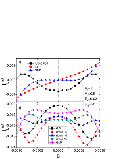
Figure 3: Panel (a): The adiabatically pumped current versus magnetic field strength $B$ for system symmetries $a$(IUD), $b$(ILR), and $d$(GUD). Curve for IUD is offset by -0.004 for a compact illustration. Panel (b): $I^{ad}$ vs $B$ for spatial symmetry GLR, GIV, and three intermediate setups. Calculation parameters: $E_{F}=0.62$, $\phi_{12}=\pi/2$, $V_{0}=1$, $V_{p}=0.5$.

Fig.3 plots the pumped current versus magnetic field strength $B$ at phase difference $\phi_{12}=\pi/2$, where the magnitude of $I^{ad}(\phi_{12})$ is maximized. In the upper panel (a) of Fig.3, we see that current is either even or odd function of magnetic field strength $B$ for symmetries IUD, ILR, and GUD, $I(B)=\pm I(-B)$ which agree with the theoretical predictions.aleiner2 ; kim In panel (b), it is clear that the pumped current is invariant upon the reversal of magnetic field for GLR.aleiner2 ; kim The system with GIV symmetry shows an approximation relation $I(B)\approx I(-B)$ only at small $B$, which is similar to that of GLR symmetry. This does not agree with the theoretical prediction.kim To further investigate the relation $I(B)\approx I(-B)$ we studied three intermediate setups between GIV and GLR. In panels (e) and (f) of Fig.1, the length of the pumped potential profile is fixed as 20 both for $V_{1}$ and $V_{2}$ in the system with $40\times 40$ mesh. Then we shift down the potential profile $V_{2}$ of the GIV symmetry 5 lattice spacing each time. After 4 shifts, the system changes from GIV to GLR symmetry and in this process three intermediate systems are generated. Numerical results shown in panel (b) of Fig.3 suggest that all these setups have the relation $I(B)\approx I(-B)$ at small magnetic fields, although there are no spatial reflection symmetries in these systems. The closer system to the GLR symmetry, the larger the magnetic field for this relation. These results suggest that the general left-right symmetry is a rather strong spatial symmetry and even a rough setup (cyan-down-triangle curve in panel (b)) can lead to an accurate invariant relation of pumped current, at least for small magnetic field. Recall the experimental result switkes of an adiabatic pump where the experimental setup can not have precise GLR symmetry, but an accurate relation $I(B)=I(-B)$ was still achieved. In addition, the amplitude of pumped current in this setup with GLR symmetry is relatively high, compared with other symmetries.

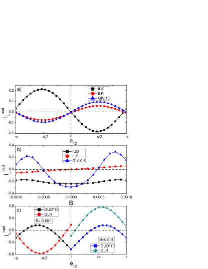
Figure 4: Panel (a): Non-adiabatically pumped current as a function of phase difference $\phi_{12}$ at a fixed magnetic field $B=0.001$ for spatial symmetries IUD, ILR, and GIV. Blue curve with up-triangle for GIV is multiplied by a factor of $0.1$. Panel (b): $I^{nad}$ versus magnetic field strength $B$ for the above three setups with $\phi_{12}=\pi/2$. Blue curve with up-triangle for GIV is offset by $-0.8$. Panel (c): The pumped current for system setups GUD and GLR. Curves for GUD are multiplied by $0.1$. Calculation parameters: $E_{F}=0.62$, $V_{0}=1$, $V_{p}=40$.

Now we turn our attention to the non-adiabatic electron pump with finite pumping frequency. The numerical results are presented in Fig.4. One of the major differences between adiabatic and non-adiabatic pump is that a non-adiabatic pump can operate with only one system parameter, since the finite pumping frequency supplies one extra degree of freedom and it could act as another pumping parameter. In the experimentswitkes it was found that $I(\phi_{12}=0)\neq 0$. Later a theoretical workbaigeng1 attributed this phenomenon as a consequence of photon-assisted processes and it is a nonlinear transport feature of non-adiabatic electron pump. In our numerical results, we also found that $I^{nad}(\phi_{12}=n\pi)\neq 0$ is a general property of the pumped current, except for systems with spatial symmetries IIV or GIV. Although the pumping frequency $\omega$ can play the role of a variation parameter, the pumped current in the system with symmetry IIV is always zero. For the setup with GIV symmetry, we see from panel (a) of Fig.4 that the pumped current obeys an antisymmetric relation with phase difference: $I^{nad}(\phi_{12})=-I^{nad}(-\phi_{12})$. $I^{nad}(\phi_{12}=n\pi)=0$ is a natural result of this antisymmetry relation. Combining with the result from the adiabatic case (Fig.2), we see that this antisymmetry relation between pumped current and phase difference $\phi_{12}$ is a general feature of the GIV symmetry. Besides, from panel (b) of Fig.4 we found that, $I^{nad}$ for GIV system at a fixed phase $\phi_{12}=\pi/2$ shows $I^{nad}(B)\approx I^{nad}(-B)$ at small magnetic field. This approximate symmetry relation can not be obtained theoretically. Our results confirm the theoretical predictions on the parity of pumped current on reversal of magnetic field for setups IUD and ILRkim , which are respectively $I(B)=I(-B)$ and $I(B)=-I(-B)$ (see panel (b)). However, it doesn’t hold for GUD and GLR in panel (c). In this case, one can only get the relations $I(B,\phi)=I(-B,-\phi)$ for GUD and $I(B,\phi)=-I(-B,-\phi)$ for GLRkim . When the two pumping potentials operate in phase or out of phase ($\phi_{12}=n\pi$), they reduce to a simple version: $I(B)=I(-B)$ for GUD and $I(B)=-I(-B)$ for GLR, which are the same for IUD and ILR at $\phi_{12}=n\pi$. It is worth mentioning that these two relations are in contrary to the adiabatic case where $\phi_{12}\neq n\pi$.

We collect the results and summarize these conclusions drawn from both adiabatic and nonadiabatic pumps and there are shown in Table.1 in detail.

	adiabatic pump		nonadiabatic pump
	$\phi_{12}=n\pi$	$\phi_{12}\neq n\pi$	$\phi_{12}=n\pi$	$\phi_{12}\neq n\pi$
IUD	${I=0}^{\diamond}$	${I(B)=I(-B)}^{\diamond}$	${I(B)=I(-B)}^{\diamond}$	${I(B)=I(-B)}^{\diamond}$
ILR	${I=0}^{\diamond}$	${I(B)=-I(-B)}^{\diamond}$	${I(B)=-I(-B)}^{\diamond}$	${I(B)=-I(-B)}^{\diamond}$
IIV	${I=0}^{\diamond}$	${I=0}^{\diamond}$	${I=0}^{\diamond}$	${I=0}^{\diamond}$
GUD	${I=0}^{\diamond}$	${I(B)=-I(-B)}^{\diamond}$	${I(B)=I(-B)}^{\diamond}$	${I(B,\phi)=I(-B,-\phi)}^{\diamond}$
GLR	${I=0}^{\diamond}$	${I(B)=I(-B)}^{\diamond}$	${I(B)=-I(-B)}^{\diamond}$	${I(B,\phi)=-I(-B,-\phi)}^{\diamond}$
GIV	${I=0}^{\diamond}$	${I\approx 0}^{\triangleright}$	${I=0}^{\diamond}$	${I(B,\phi)=-I(B,-\phi)}^{\diamond}$
		${I(B)\approx I(-B)}^{\ast}$		${I(B)\approx I(-B)}^{\ast}$

Table 1: Symmetry of the pumped currents on inversion of the magnetic field for both adiabatic and nonadiabatic electron pumps.
    $\diamond$ stands for the theoretical prediction from Ref.kim, confirmed by our numerical calculation.
$\triangleright$ represents theoretical relation without numerical sustainment.
$\ast$ corresponds to our new finding in contrast to the theoretical prediction.

III.2 Transport properties of the pumped current

In the last section we have concentrated on the symmetry of the pumped current with magnetic field $B$ and phase difference $\phi_{12}$ as the variables. Now we study the effect of other system parameters on the pumped current. Numerical calculations were performed on a system with instant L-R symmetry (ILR), in which widths of the four potential barriers are kept equal. The numerical results are plotted in Fig.5, Fig.6 and Fig.7.

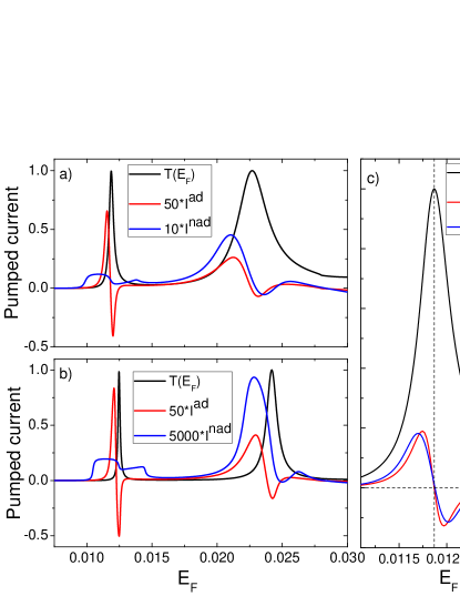
Figure 5: Panel (a) and (b): The pumped current as well as transmission coefficient as a function of Fermi energy at static potential height $V_{0}=1.0$ and $V_{0}=5.0$, respectively. For visualization purpose, a factor is multiplied to the pumped current in Fig.5. For $I^{ad}$ the factor is 50 in both panels. For $I^{nad}$ this factor is 10 in panel (a) and 5000 in panel (b). Other parameters: $B=0.001$, $\phi_{12}=\pi/2$. $V_{p}=0.5$, $\omega=0.002$ in panel (a) and $V_{p}=4.5$, $\omega=0.002$ in panel (b). Panel (c) highlights the pumped current at small pumping amplitudes at the first resonant peak. $V_{0}=1.0$ in this panel and $V_{p}=0.05$, $\omega=0.0002$. The factors for $I^{ad}$ and $I^{nad}$ are 1000 and 10, respectively.

In panel (a) of Fig.5 we plot the pumped current in the presence of magnetic field as a function of Fermi energy $E_{F}$, together with the transmission coefficient $T(E_{F})$ at static potential barrier $V_{0}=1.0$. The sharp tips of transmission coefficient suggests that quantum resonance effect dominates the transport process. When a dc bias is applied, the tunneling current is calculated from transmission profile. However, the pumped current is generated as zero bias by periodically varying ac gate voltages. Although originating from different physical mechanisms, we see that the pumped current clearly show resonance characteristics both in adiabatic and non-adiabatic cases near the resonant energy of static transmission coefficient. These resonance-assisted behavior of pumped current is a generic property of electron pump.ydwei1 Operating at the coherent regime, quantum interference naturally results in its resonant behavior. It is worth mentioning that near the sharp resonance at $E_{F}=0.0118$ the adiabatic pumped current changes sign. This is understandable. In the presence of dc bias, the direction of the current is determined by the bias. For parametric electron pump at zero bias, the direction of the pumped current depends only on the system parameters such as Fermi energy and magnetic field. Variation of these parameters can change the current direction. For the non-adiabatic pump, the pumped current changes slowly near the resonance but there is no sign changes for the pumped current. In Fig.5(a), we also see a second resonant point with much broader peak. Near this resonant level, we see that the transmission coefficient and the pumped currents are well correlated. The resonant feature of the pumped current is also related to the width of the resonant peak in the transmission coefficient. Similar behaviors are found for a higher static potential barrier $V_{0}=5.0$ in panel (b). A larger barrier makes the resonant peaks much sharper, but it doesn’t qualitatively affect the pumped current. The noticeable difference is that, the pumped current peaks are shifted with that of the transmission coefficient. In addition, it seems that the non-adiabatic pumped current develops a plateau region near the first resonant peak.

When zooming in at this resonant peak ($E=0.0118$ in Fig.5(a)), we found that at small pumping amplitude the pumped currents are zeros for both adiabatic and non-adiabatic cases when a complete transmission occurs (transmission coefficient $T=1$). The numerical evidence is shown in panel (c) of Fig.5. Note that there is only one transmission channel for the incident energy so that $T=1$ corresponds to complete transmission. We emphasize that the non-adiabatic pumped current goes to zero near the resonance only for very small frequency. At larger frequency such as the case in Fig.5(a) or (b), it is nonzero. For the case of $I^{ad}$, it is easy to understand why it is zero at $T=1$. For a perfect transmission, the diagonal terms $S_{LL}$ and $S_{RR}$ of the four-block scattering matrix are zero. Hence we have $S_{LR}=S_{RL}=\exp(i\theta)$. From Eq.(2), we have

$$dN_{\alpha}/dV_{j}=(i\partial\theta/\partial V_{j})/\pi$$ (7)

For two pumping potentials, the current can be expressed in parameter space. Using the Green’s theorem, Eq.(1) becomesbrouwer1 ,

$$I_{\alpha} = \frac{1}{\tau}\int_{0}^{\tau}dt\frac{dQ_{\alpha}(t)}{dt}$$ (8)

$$= \frac{q\omega}{2\pi}\int dV_{1}dV_{2}\left(\frac{\partial}{\partial V_{1}}\frac{dN_{\alpha}}{dV_{2}}-\frac{\partial}{\partial V_{2}}\frac{dN_{\alpha}}{dV_{1}}\right)$$

From Eq.(7), it is easy to see that the integrand is zero. Hence $I_{\alpha}=0$ if $S_{\alpha\alpha}=0$. For non-adiabatic case, the pumped current at complete transmission is in general nonzero. However, if the frequency is very small, the adiabatic case is recovered. This is numerically supported by Fig.5(c), where the two current curves are very similar.

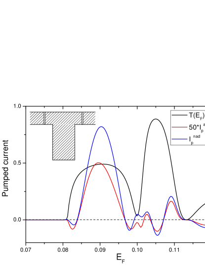
Figure 6: The pumped current versus Fermi energy in a T-shaped system. The side bar is of length 20 and width 30. Two gray blocks indicate the positions where the pumping potentials are applied and the static potential is set to be zero. A factor of 50 is multiplied to $I^{ad}$. Other parameters: $B=0.001$, $\phi_{12}=\pi/2$. $V_{p}=0.05$, $\omega=0.002$.

Furthermore, the behavior of pumped current for a structure exhibiting anti-resonance phenomena was studied and the numerical results is shown in Fig.6. To establish anti-resonance, we use a T-junctionT-junction , which is schematically plotted in the inset of Fig.6. The side bar has longitudinal dimension 20 and transverse dimension 30. Pumping potentials are placed on the two arms of the device and there are no static potential barriers in the system. From the transmission curve shown in Fig.6, one clearly finds that $T(E_{F})$ drops sharply to zero around $E_{F}=0.112$, which is the signature of anti-resonance. At this point, both the adiabatic and nonadiabatic pumped current are zero. Different from the resonant case, here the range where the current is zero or nearly zero is much broader. The phenomena are attributed to reasons similar to those we presented above, but in this case $S_{LR}$ and $S_{RL}$ are zero at the anti-resonance point. We also see that at transmission minimum $E_{F}=0.10$ with small transmission coefficient the pumped current is nonzero.

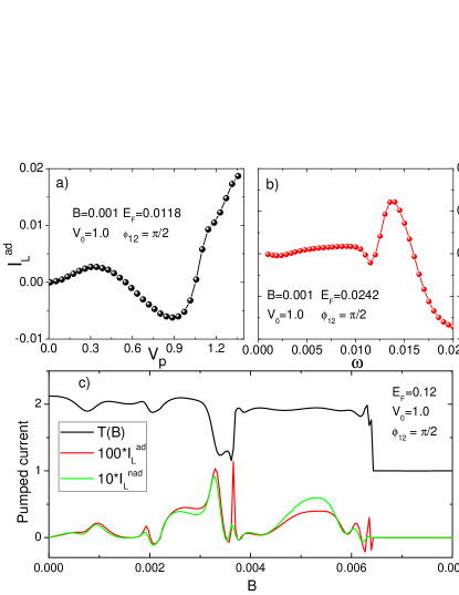
Figure 7: Panel (a): Adiabatic current vs pumping potential $V_{p}$ at $E_{F}=0.0118$. Panel (b): Non-adiabatic current versus pumping frequency $\omega$ at $E_{F}=0.0242$. System parameters: $\phi_{12}=\pi/2$, $V_{0}=1$, $B=0.001$. Panel (c) shows the pumped current and transmission coefficient versus magnetic field $B$ at Fermi energy $E_{F}=0.12$, with other parameters: $\phi_{12}=\pi/2$, $V_{0}=1$, $V_{p}=0.5$, $\omega=0.002$. For illustration a factor of 100 is multiplied to $I^{ad}$ and it is 10 for $I^{nad}$.

In panel (a) and (b) of Fig.7, we examine the influence of pumping amplitude $V_{p}$ on the pumped currents with the static potential barrier fixed at $V_{0}=1$, which corresponds to the case shown in panel (a) of Fig.5. At the first resonant energy $E_{F}=0.0118$ we plot $I^{ad}$ versus $V_{p}$, the pumping potential amplitude. The non-adiabatic pumped current $I^{nad}$ as a function of the pumping frequency $\omega$ is evaluated at the second resonant peak $E_{F}=0.0242$. In both cases, magnitudes of the pumped current changes in a oscillatory fashion with the increasing of $V_{p}$ or $\omega$. The pumped current can change its sign, which also reflects the nature of the parametric pump and manifest distinction between the pumped current and the conventional resonant tunneling current.

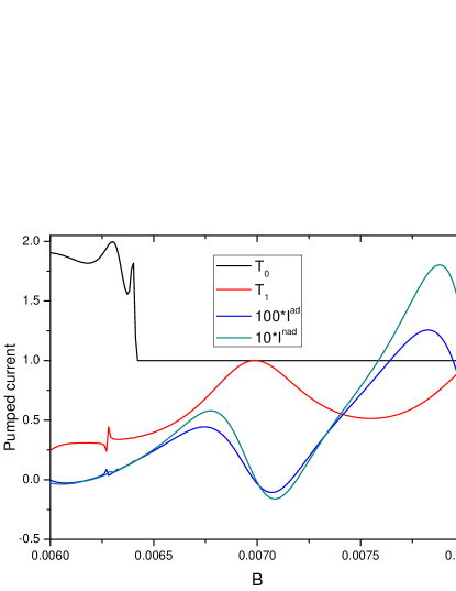
Figure 8: The pumped current as well as transmission coefficient as a function of magnetic field $B$ at Fermi energy $E_{F}=0.12$. Other parameters: $\phi_{12}=\pi/2$, $V_{0}=1$, $V_{p}=0.5$, $\omega=0.002$. $I^{ad}$ and $I^{nad}$ are scaled by factors of 100 and 10, respectively.

The resonance behavior of pumped current is also visible in panel (c) of Fig.7, in which we depict $I_{p}$ and transmission coefficient versus magnetic field $B$ at Fermi energy $E_{F}=0.12$. Sweeping through magnetic field, there is a sharp change of transmission coefficient near $B\sim 0.003$ and the pumped current changes accordingly. With increasing magnetic field, $T$ becomes quantized (there is only one transmission channel at this magnetic field) indicating the occurrence of edge states in the quantum Hall regime and the pumped current vanishes. In our setup, electron pump operates by cycling modulation of electron passing through the pumping potentials which are on top of static barriers defining the system. With increasing of the magnetic field, electron wavefunction tends to localize near the edge, which decreases the modulation efficiency of the pumping potentials. As the edge state emerges, electron will circumvent the confining potentials with no reflection during their deformations. In this case, the variation of pumping potential has no effect on the moving electron. Hence there is no pumped current when edge state is formed in the system. Mathematically it is also easy to show from Eq.(1) that for a two-probe system as long as the instantaneous reflection coefficient vanishes (in the case of edge state) in the whole pumping period there is no adiabatic pumped current.

We provide a numerical evidence for the above statement, which is shown in Fig.8. In contrast to the calculation of panel (c) of Fig.7, the static potential barriers extend to a width 40, which is exactly the width of the scattering region. At the same time, the pumping barriers remain the same as before (with width 10). Now the static transmission coefficient, labeled $T_{1}$ in the figure, does not have quantized value but exhibits a resonant behavior. $T_{0}$ is copied from Fig.7 for comparison. As long as the edge state of an electron is scattered with transmitted and reflected modes, the pumped current will be generated with varying system parameters.

IV conclusion

In conclusion, we have studied the pumped current as a function of pumping potential, magnetic field and pumping frequency in the resonant and anti-resonant tunneling regimes. Resonant features are clearly observed for adiabatic and non-adiabatic pumped current. We found that when the resonant peak is sharp the adiabatic pumped current changes sign near the resonance while non-adiabatic pumped current does not. When the resonant peak is broad the behaviors of pumped current in adiabatic and non-adiabatic regimes are similar and both change sign near the resonance. At anti-resonance, however, both adiabatic and non-adiabatic pumped current are zero. As the system enters the quantum Hall regime, pumped currents vanishes in all the setups shown in Fig.1, since the pumping potentials can not modulate the electron wave function. Furthermore, we have numerically investigated the symmetry of the adiabatic and non-adiabatic pumped current of systems with different symmetries placed in magnetic field. The calculated results are listed in Table.1 and most of them are in agreement with the former theoretical results derived from Floquet scattering matrix theory. Different from the theoretical prediction, we found that the system with general spatial inversion symmetry (GIV) gives rise to a finite pumped current at adiabatic regime. At small magnetic field, both the adiabatic and non-adiabatic currents have an approximation relation $I(B)\approx I(-B)$.

V acknowledgments

This work is supported by RGC grant (HKU 705409P), University Grant Council (Contract No. AoE/P-04/08) of the Government of HKSAR, and LuXin Energy Group. The computational work is partially performed on HPCPOWER2 system of the computer center, HKU.

References

- (1) D. J. Thouless, Phys. Rev. B 27, 6083 (1983).
- (2) Q. Niu and D.J. Thouless, J. Phys. A 17, 2453 (1984).
- (3) Q. Niu, Phys. Rev. Lett. 64, 1812 (1990).
- (4) F. Hekking and Yu. V. Nazarov, Phys. Rev. B 44, 9110 (1991).
- (5) T. A. Shutenko, I. L. Aleiner, and B. L. Altshuler, Phys. Rev. B 61, 10366 (2000).
- (6) S. W. Chung, C. S. Tang, C. S. Chu, and C. Y. Chang, Phys. Rev. B 70, 085315 (2004).
- (7) I. L. Aleiner and A. V. Andreev, Phys. Rev. Lett. 81, 1286 (1998).
- (8) M. Switkes, C. M. Marcus, K. Campman, and A.C. Gossard, Science 283, 1907 (1999).
- (9) Y. Wei, J. Wang, H. Guo, and C. Roland, Phys. Rev. B 64, 115321 (2001).
- (10) V.I. Talyanskii, D.S. Novikov, B.D. Simons, and L.S. Levitov, Phys. Rev. Lett. 87, 276802 (2001).
- (11) Zhu and H. Chen, Appl. Phys. Lett. 95, 122111 (2009).
- (12) Q. Zhang, K. S. Chan, and Z. Lin, Appl. Phys. Lett. 98, 032106 (2011).
- (13) S. K. Watson, R. M. Potok, C. M. Marcus, and V. Umansky, Phys. Rev. Lett. 91, 258301 (2003).
- (14) A. G. Malshukov, C. S. Tang, K. S. Chu, and K. A. Chao, Phys. Rev. B 68, 233307 (2003).
- (15) R. Benjamin and C. Benjamin, Phys. Rev. B 69, 085318 (2004).
- (16) M. Swikes, Ph.D thesis, Stanford University, 1999.
- (17) P. W. Brouwer, Phys. Rev. B 58, R10135 (1998).
- (18) P. W. Brouwer, Phys. Rev. B 63, 121303 (2001).
- (19) A. Andreev and A. Kamenev, Phys. Rev. Lett. 85, 1294 (2000).
- (20) S. W. Kim, Phys. Rev. B 66, 235304 (2002).
- (21) M. Moskalets and M. Büttiker, Phys. Rev. B. 66, 205320 (2002).
- (22) B. Wang, J. Wang, and H. Guo, Phys. Rev. B. 65, 073306 (2002).
- (23) B. Wang, J. Wang, and H. Guo, Phys. Rev. B. 68, 155326 (2003).
- (24) O. Entin-Wohlman and A. Aharony, Phys. Rev. B 66, 035329 (2002).
- (25) A. Agarwal and D. Sen, J. Phys.: Condens. Matter 19, 046205 (2007).
- (26) F. Zhou, B. Spivak, and B. L. Altshuler, Phys. Rev. Lett. 82, 608 (1999).
- (27) Y. Wei, J. Wang, and H. Guo, Phys. Rev. B 62, 9947 (2000).
- (28) I. L. Aleiner, B. L. Altshuler and A. Kamenev, Phys. Rev. B. 62, 10373 (2000).
- (29) S. W. Kim, Phys. Rev. B. 68, 085312 (2003).
- (30) M. Moskalets and M. Büttiker, Phys. Rev. B. 72, 035324 (2005).
- (31) C. Li, Y. Yu, Y. Wei, and J. Wang, Phys. Rev. B. 75, 035312 (2007).
- (32) F. Sols, M. Macucci, U. Ravaioli, and K. Hess, Appl. Phys. Lett. 54, 350 (1989).