Second order expansions of distributions of maxima of bivariate Gaussian triangular arrays under power normalization

Abstract. In this paper, we study second order expansions of distributions of maxima of bivariate Gaussian triangular arrays under power normalization. Numerical analysis are given to compare the asymptotic behaviors under power normalization with the asymptotic behaviors under linear normalization derived by Hashorva et al. (2016).

keywords: Second order expansion; Maximum; Bivariate Gaussian triangular array; Power normalization

1 Introduction

Let $\{(X_{n,k},Y_{n,k}),1\leq k\leq n,n\geq 1\}$ be a triangular array of independent standard bivariate Gaussian random vector with correlations $\{\rho_{n},n\geq 1\}$ and joint distribution function $F$. Hüsler and Reiss (1989) considered the asymptotic behavior of distribution of maxima with correlation coefficient varying as the sample size increases. Under the so-called Hüsler-Reiss condition

$$\lim_{n\to\infty}\frac{1}{2}b_{n}^{2}(1-\rho_{n})=\lambda^{2}$$ (1.1)

with $\lambda\in[0,\infty]$, Hüsler and Reiss (1989) showed that

$$\lim_{n\to\infty}\sup_{x,y\in\mathbb{R}}|F^{n}(b_{n}+x/b_{n},b_{n}+y/b_{n})-H_{\lambda}(x,y)|=0$$

holds, where the norming constant $b_{n}$ is given by

$$n(1-\Phi(b_{n}))=1,$$ (1.2)

with $\Phi$ standing for the standard Gaussian distribution, and the max-stable Hüsler-Reiss distribution $H_{\lambda}$ is given by

$$H_{\lambda}(x,y)=\exp\left(-\Phi(\lambda+\frac{x-y}{2\lambda})e^{-y}-\Phi(\lambda+\frac{y-x}{2\lambda})e^{-x}\right),\quad x,y\in\mathbb{R}$$

with $H_{0}(x,y)=\exp\left(-e^{-\min(x,y)}\right)$ and $H_{\infty}(x,y)=\Lambda(x)\Lambda(y)$ with $\Lambda(x)=\exp\left(-e^{-x}\right)$, $x\in\mathbb{R}$.

Extensions the work of Hüsler and Reiss (1989) can be found in recent literature. Hashorva (2005, 2006) considered the case of triangular arrays of independent elliptical random vectors, Hashorva and Ling (2016) extended the results to the case of bivariate skew-normal triangular array. Motivated by the work of Nair (1981) and Frick and Reiss (2013), for the Hüser-Reiss model Hashorva et al. (2016) established the higher-order expansions of distributions of maxima under the refined Hüsler-Reiss conditions and Liao and Peng (2014) considered its associated uniform convergence rates.

In this paper, we are interested in the rate of convergence of the distribution of maxima of Hüsler-Reiss model under power normalization. For univariate case, it’s well known that

$$\lim_{n\to\infty}\sup_{x\in\mathbb{R}}|\Phi^{n}(b_{n}+x/b_{n})-\Lambda(x)|=0$$

holds with $b_{n}$ given by (1.2), cf. Resnick (1987) and Nair (1981). In view of Mohan and Ravi (1993), let $\alpha_{n}=b_{n}$ and $\beta_{n}=b_{n}^{-2}$, we have

$$\lim_{n\to\infty}\Phi^{n}(b_{n}x^{b_{n}^{-2}})=\Phi_{1}(x),$$ (1.3)

where $\Phi_{1}(x)=\exp\left(-x^{-1}\right),x>0$, one of six-type power-stable distributions given by Pancheva(1985). For recent work on maxima under power normalization, see Mohan and Subramanya (1991), Mohan and Ravi (1993), Subramanya (1994), Barakat et al. (2010) and Peng et al. (2013). In this paper we will show that under the Hüsler-Reiss condition (1.1)

$$\lim_{n\to\infty}\sup_{x,y>0}|F^{n}(b_{n}x^{b_{n}^{-2}},b_{n}y^{b_{n}^{-2}})-H_{\lambda}(\ln x,\ln y)|=0$$ (1.4)

holds with $H_{0}(\ln x,\ln y)=\exp\left(-(\min(x,y))^{-1}\right)$ and $H_{\infty}(\ln x,\ln y)=\exp\left(-x^{-1}\right)\exp\left(-y^{-1}\right)$. Furthermore, the rate of convergence in (1.3) and (1.4) will be investigated, respectively.

The rest of the paper is organized as follows. In Section 2 we present the main results. Numerate analysis provided in Section 3 compare the asymptotic behaviors under power and linear normalization. All the proof are relegated to Section 4.

2 Main results

In this section, we provide the main results with respect to limiting distribution of maxima under power normalization under the Hüsler-Reiss condition (1.1) and its second-order expansions providing some refined Hüsler-Reiss condition hold. In the following we shall denote throughout by $b_{n}$ the constants defined in (1.2). First we state (1.4) as the following result.

Theorem 2.1.

For the considered bivariate Gaussian triangular array, the Hüsler-Reiss condition (1.1) holds if and only if (1.4) holds.

To establish the higher-order expansion of the distribution of maxima in Hüsler-Reiss model, we need to refine the Hüsler-Reiss condition (1.1). There are three cases to be considered, i.e., $\lambda\in(0,\infty)$, $\lambda=0$ and $\lambda=\infty$, respectively.

For $\lambda\in(0,\infty)$, the result is given as follows.

Theorem 2.2.

If the second-order Hüsler-Reiss condition

$$\lim_{n\to\infty}b_{n}^{2}(\lambda-\lambda_{n})=\tau\in\mathbb{R}$$ (2.1)

holds with $\lambda_{n}=(\frac{1}{2}b_{n}^{2}(1-\rho_{n}))^{1/2}$ and $\lambda\in(0,\infty)$, then for $x>0$, $y>0$ we have

$$\lim_{n\to\infty}b_{n}^{2}\left(F^{n}(b_{n}x^{b_{n}^{-2}},b_{n}y^{b_{n}^{-2}})-H_{\lambda}(\ln x,\ln y)\right)=\kappa(x,y,\lambda,\tau)H_{\lambda}(\ln x,\ln y)$$ (2.2)

with $\kappa(x,y,\lambda,\tau)$ given by (4.13).

Remark 2.1.

(i) Let $\gamma_{n}=(\lambda-\lambda_{n})^{-1}$. If (2.1) does not converge but $\gamma_{n}$ and $b_{n}^{2}$ are the same order, then $b_{n}^{-2}$ and $F^{n}\left(b_{n}x^{b_{n}^{-2}},b_{n}y^{b_{n}^{-2}}\right)-H_{\lambda}(\ln x,\ln y)$ are the same order.

(ii) If $\lim_{n\to\infty}b_{n}^{2}/\gamma_{n}=\pm\infty$, with arguments similar to that of Theorem 2.2, we can show that

$$\lim_{n\to\infty}\gamma_{n}\left(F^{n}\left(b_{n}x^{b_{n}^{-2}},b_{n}y^{b_{n}^{-2}}\right)-H_{\lambda}(\ln x,\ln y)\right)=2x^{-1}\varphi\left(\lambda+\frac{\ln\frac{y}{x}}{2\lambda}\right)H_{\lambda}(\ln x,\ln y).$$ (2.3)

(iii) Conversely, for the bivariate Gaussian triangular arrays with correlations $\{\rho_{n}\}$ satisfying (1.1), we have the following assertions under power normalization: (a) if (2.2) holds, then (2.1) holds. (b) if $F^{n}\left(b_{n}x^{b_{n}^{-2}},b_{n}y^{b_{n}^{-2}}\right)-H_{\lambda}(\ln x,\ln y)$ and $b_{n}^{-2}$ are the same order, then $\gamma_{n}$ and $b_{n}^{2}$ are the same order. (c) if (2.3) holds, then $\lim_{n\to\infty}b_{n}^{2}/\gamma_{n}=\pm\infty$. (d) if $F^{n}\left(b_{n}x^{b_{n}^{-2}},b_{n}y^{b_{n}^{-2}}\right)-H_{\lambda}(\ln x,\ln y)$ and $\gamma_{n}$ are the same order, then $\gamma_{n}$ and $b_{n}^{2}$ are the same order.

Remark 2.2.

For the case of $\lambda\in(0,\infty)$, if (2.1) does not converge, and $\gamma_{n}$ and $b_{n}^{2}$ are not the same order, there may be no convergence rates for the extremes. An example is: suppose that the bivariate Gaussian triangular arrays have correlations $\{\rho_{n}\}$ satisfying (1.1). Furthermore, assume that $\lim_{n\to\infty}b_{2n}^{2}/\gamma_{2n}=0$ and $\lim_{n\to\infty}b_{2n+1}^{2}/\gamma_{2n+1}=\infty$. Hence, by Theorem 2.2 and Remark 2.1 (ii), we have

$$\lim_{n\to\infty}b_{2n}^{2}\left(F^{2n}\left(b_{2n}x^{b_{2n}^{-2}},b_{2n}y^{b_{2n}^{-2}}\right)-H_{\lambda}(\ln x,\ln y)\right)=\kappa(x,y,\lambda,0)H_{\lambda}(\ln x,\ln y)$$

and

$$\lim_{n\to\infty}\gamma_{2n+1}\left(F^{2n+1}\left(b_{2n+1}x^{b_{2n+1}^{-2}},b_{2n+1}y^{b_{2n+1}^{-2}}\right)-H_{\lambda}(\ln x,\ln y)\right)=2x^{-1}\varphi\left(\lambda+\frac{\ln\frac{y}{x}}{2\lambda}\right)H_{\lambda}(\ln x,\ln y).$$

Next we give the results of two extreme cases: $\lambda=\infty$ and $\lambda=0$ with different refined conditions. The following theorem considers the case of $\lambda=\infty$.

Theorem 2.3.

For $\rho_{n}\in[-1,1)$, assume that $\lim_{n\to\infty}\frac{\ln b_{n}}{b_{n}^{2}(1-\rho_{n})}=0$. Then for all $x>0$, $y>0$ we have

$$\lim_{n\to\infty}b_{n}^{2}\left(F^{n}(b_{n}x^{b_{n}^{-2}},b_{n}y^{b_{n}^{-2}})-H_{\infty}(\ln x,\ln y)\right)=(s(x)+s(y))H_{\infty}(\ln x,\ln y)$$ (2.4)

with $s(x)$ given by (4.1).

For the case of $\lambda=0$, we have the following result.

Theorem 2.4.

For $\rho_{n}\in(0,1]$, assume that $\lim_{n\to\infty}b_{n}^{6}(1-\rho_{n})=0$. Then for $x>0$, $y>0$ we have

$$\lim_{n\to\infty}b_{n}^{2}\left(F^{n}(b_{n}x^{b_{n}^{-2}},b_{n}y^{b_{n}^{-2}})-H_{0}(\ln x,\ln y)\right)=s(\min(x,y))H_{0}(\ln x,\ln y)$$ (2.5)

with $s(x)$ given by (4.1).

3 Numerical analysis

In this section, numerical studies are presented to illustrate the accuracy of second order expansions of $F^{n}$ under two different normalization, i.e., the finite behaviors under power normalization derived in this paper and that under linear normalization given by Hashorva et al. (2016). We shall discuss three particular cases:
$(i)$ $\lambda\in(0,\infty)$ with

$$\rho_{n}=1-\frac{2\lambda^{2}}{b_{n}^{2}}+\frac{4\tau\lambda}{b_{n}^{4}}-\frac{2\tau^{2}}{b_{n}^{6}},$$ (3.1)

where $b_{n}$ satisfies (1.2), which implies that condition (2.1) holds;
$(ii)$ $\rho_{n}=-1,0$ implying $\lambda=\infty$;
$(iii)$ $\rho_{n}=1$ implying $\lambda=0$.

For the case of power normalization, we calculate the actual values $F^{n}(b_{n}x^{b_{n}^{-2}},b_{n}y^{b_{n}^{-2}})$, the first-order asymptotics $L_{1}^{p}=H_{\lambda}(\ln x,\ln y)$, the second-order asymptotics according to the values of $\rho_{n}$ with finite $n$, i.e.,

• if $\rho_{n}$ is given by (3.1) with fixed $\lambda$ and $\tau$, then in view of (2.2) the second-order asymptotics are given by $L_{2}^{p}=H_{\lambda}(\ln x,\ln y)\left(1+b_{n}^{-2}\kappa(x,y,\lambda,\tau)\right)$;

• if $\rho_{n}=-1,0$, by (2.4) the second-order asymptotics are given by $L_{3}^{p}=H_{\infty}(\ln x,\ln y)\left(1+b_{n}^{-2}(s(x)+s(y))\right)$; and

• if $\rho_{n}=1,n\geq 1$ by (2.5) the second-order asymptotics are given by $L_{4}^{p}=H_{0}(\ln x,\ln y)\left(1+b_{n}^{-2}s(\min(x,y))\right)$.

For the linear normalization case, by Theorem 2.1 and Theorem 2.3 in Hashorva et al. (2016), we have the first-order asymptotics $L_{1}^{l}=H_{\lambda}(x,y)$, the second-order asymptotics according to the values of $\rho_{n}$ with finite $n$, i.e.,

• if $\rho_{n}$ is given by (3.1) with fixed $\lambda$ and $\tau$, then the second-order asymptotics are given by $L_{2}^{l}=H_{\lambda}(x,y)(1+b_{n}^{-2}\iota(x,y,\lambda,\tau))$;

• if $\rho_{n}=-1,0$, the second-order asymptotics are given by $L_{3}^{l}=H_{\infty}(x,y)\left(1+b_{n}^{-2}(\omega(x)+\omega(y))\right)$; and

• if $\rho_{n}=1,n\geq 1$ the second-order asymptotics are given by $L_{4}^{l}=H_{0}(x,y)\left(1+b_{n}^{-2}\omega(\min(x,y))\right)$,

where $\omega(x)$ and $\iota(x,y,\lambda,\tau)$ are given by

$$\omega(x)=2^{-1}(x^{2}+2x)e^{-x},$$

$$\iota(x,y,\lambda,\tau)=\omega(x)\Phi(\lambda+\frac{y-x}{2\lambda})+\omega(y)\Phi(\lambda+\frac{x-y}{2\lambda})+(2\tau-\lambda(\lambda^{2}+x+y+2))e^{-x}\varphi(\lambda+\frac{y-x}{2\lambda}).$$

To compare the accuracy of actual values with its asymptotics, let $\Delta_{i}^{p}=|F^{n}(b_{n}x^{b_{n}^{-2}},b_{n}y^{b_{n}^{-2}})-L_{i}^{p}|$ and $\Delta_{i}^{l}=|F^{n}(b_{n}+x/b_{n},b_{n}+y/b_{n})-L_{i}^{l}|$, $i=1,2,3,4$ denote the absolute errors under power and linear normalization, respectively. We use $\mathbf{R}$ to calculate the absolute errors with sample sizes $n=1000$ and $n=10000$, and fixed $\lambda$, $\tau$, which are documented Table 1-4. These tables show that accuracies of the first and the second order asymptotics under two different normalization can be improved as $n$ becomes large.

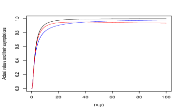
(b) $\lambda=2.5,\tau=-5,\rho_{n}=-0.915$

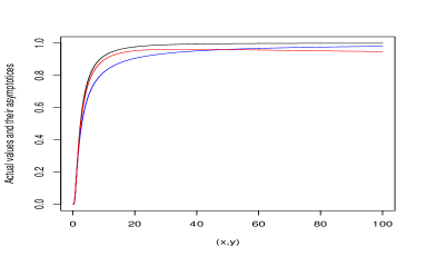
(c) $\lambda=2.5,\tau=-2,\rho_{n}=-0.537$

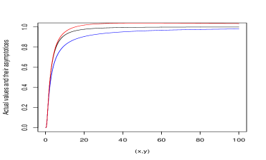
(d) $\rho_{n}=0$

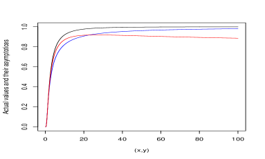
(e) $\lambda=2,\tau=2,\rho_{n}=0.329$

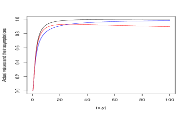
(f) $\lambda=2,\tau=3,\rho_{n}=0.405$

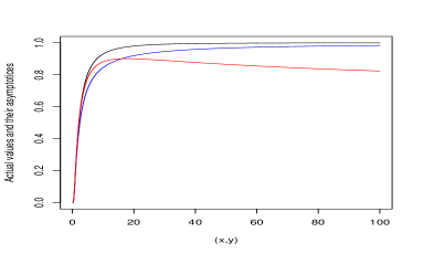
(g) $\lambda=1,\tau=2,\rho_{n}=0.869$

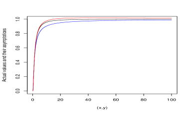
(h) $\rho_{n}=1$

Figure 1: Actual values and its approximations with $n=10^{3},x=y\in[0,100]$. The actual values with black color, the first-order asymptotics with blue color, the second-order asymptotics with red color.

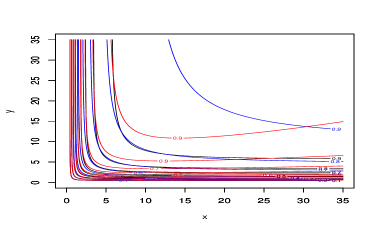
(b) $\lambda=2.5,\tau=-5,\rho_{n}=-0.915$

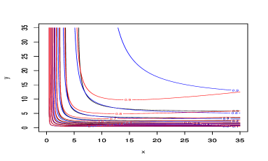
(c) $\lambda=2.5,\tau=-2,\rho_{n}=-0.537$

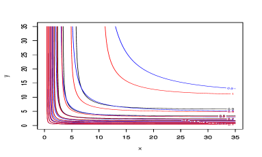
(d) $\rho_{n}=0$

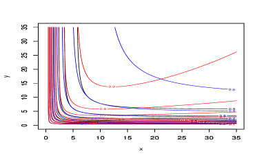
(e) $\lambda=2,\tau=2,\rho_{n}=0.329$

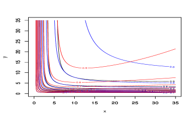
(f) $\lambda=2,\tau=3,\rho_{n}=0.405$

(g) $\lambda=1,\tau=2,\rho_{n}=0.869$

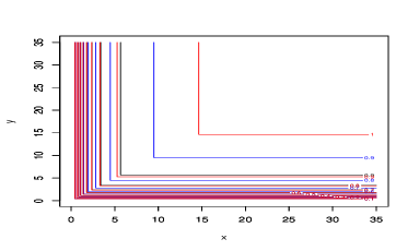
(h) $\rho_{n}=1$

Figure 2: The contour line of actual values and its approximations with $n=10^{3},x,y\in[0,35]$. The actual values with black color, the first-order asymptotics with blue color, the second-order asymptotics with red color.

In order to show the accuracy of all asymptotics with varying $x$ and $y$, we plot the actual values and its asymptotics with fixed $\lambda$, $\tau$ and $n=10^{3}$ by using $\mathbf{R}$. Power normalization cases are illustrated in Figures 1 and 2, where Figure 1 compares the actual values with above three asymptotics with $x=y$, Figure 2 compares the difference of the actual value with above three asymptotics by contour line in the plane. The cases of linear normalization are illustrated in Figures 1 and 2 in Hashorva et al. (2016).

According to Figures 1-2 in Hashorva et al. (2016), Figures 1-2 and Tables 1-4, we have the following findings: i) The asymptotics under linear normalization are more closer to its actual values except small $x$. ii) Under two different normalization, the second order asymptotics are closer to the actual values as small $x$ except few special cases, contrary to the case of large $x$, which shows that the first order asymptotics may be better.

Table 1: A̧bsolute errors between actual values and their asymptotics for the case of $\lambda=2$, $\tau=3$

(x,y)	n=1000				n=10000
	$\Delta_{1}^{p}$	$\Delta_{1}^{l}$	$\Delta_{2}^{p}$	$\Delta_{2}^{l}$	$\Delta_{1}^{p}$	$\Delta_{1}^{l}$	$\Delta_{2}^{p}$	$\Delta_{2}^{l}$
(0.5,0.5)	0.00133	0.01646	0.00078	0.00114	0.00106	0.01128	0.00039	0.0007
(1,1)	0.00239	0.04272	0.00241	0.00217	0.00197	0.03001	0.00135	0.00098
(1,0.5)	0.00233	0.02723	0.00192	0.00022	0.00186	0.01897	0.00108	0.00001
(2,1)	0.00901	0.05237	0.00874	0.00675	0.00598	0.03752	0.00579	0.0033
(3,3)	0.07201	0.04517	0.02066	0.01957	0.04978	0.03459	0.01432	0.01011
(3,5)	0.08486	0.0289	0.01672	0.01684	0.05934	0.02264	0.01229	0.00895
(2,3)	0.05262	0.05552	0.01079	0.01649	0.03623	0.04132	0.00735	0.00839
(5,5)	0.09987	0.01059	0.03115	0.01225	0.07058	0.00899	0.02314	0.00679
(5,9)	0.10039	0.00556	0.02004	0.00712	0.07231	0.00475	0.01684	0.004
(10,10)	0.09729	0.00009	0.04002	0.00046	0.07223	0.00009	0.03268	0.00029
(10,20)	0.08437	0.00005	0.02078	0.00024	0.06431	0.00004	0.02041	0.00015
(7,10)	0.10072	0.00091	0.02716	0.00231	0.07369	0.00084	0.02289	0.00138
(20,20)	0.06994	4.02$\times 10^{-9}$	0.05106	8.78$\times 10^{-8}$	0.05534	4.03$\times 10^{-9}$	0.04229	5.96$\times 10^{-8}$
(20,2)	0.05271	0.03781	0.10129	0.0117	0.03855	0.02808	0.07209	0.0061
(25,20)	0.06519	2.07$\times 10^{-9}$	0.06472	4.57$\times 10^{-8}$	0.05211	2.07$\times 10^{-9}$	0.05178	3.09$\times 10^{-8}$
(50,50)	0.0351	0	0.07716	0	0.03036	0	0.0594	0
(50,8)	0.07247	0.00033	0.16596	0.00108	0.05529	0.00031	0.11985	0.00066
(60,50)	0.03254	0	0.09167	0	0.02837	0	0.06919	0
(100,100)	0.01879	0	0.10239	0	0.01724	0	0.07495	0
(4,100)	0.06559	0.01236	0.00823	0.01024	0.04804	0.01003	0.00293	0.00557
(100,4)	0.06559	0.01236	0.26446	0.01024	0.04804	0.01003	0.18535	0.00557
(150,100)	0.01579	0	0.14059	0	0.01465	0	0.10082	0
(200,200)	0.00965	0	0.12808	0	0.00924	0	0.09101	0
(200,320)	0.00787	0	0.10243	0	0.00759	0	0.0729	0
(4,200)	0.06242	0.01236	0.00869	0.01024	0.0453	0.01003	0.00379	0.00557
(200,4)	0.06242	0.01236	0.35623	0.01024	0.0453	0.01003	0.24816	0.00557

Table 2: A̧bsolute errors between actual values and their asymptotics for the case of $\rho=-1$

(x,y)	n=1000				n=10000
	$\Delta_{1}^{p}$	$\Delta_{1}^{l}$	$\Delta_{3}^{p}$	$\Delta_{3}^{l}$	$\Delta_{1}^{p}$	$\Delta_{1}^{l}$	$\Delta_{3}^{p}$	$\Delta_{3}^{l}$
(0.5,0.5)	0.00112	0.02047	0.00051	0.00314	0.00079	0.01474	0.00033	0.00156
(1,1)	0.00027	0.04775	0.00027	0.00763	0.00003	0.0343	0.00003	0.00393
(1,0.5)	0.00156	0.03177	0.00065	0.00502	0.00109	0.02285	0.00044	0.00256
(2,1.5)	0.02903	0.0664	0.00249	0.01606	0.02051	0.04861	0.00125	0.00833
(3,3)	0.07729	0.04709	0.00535	0.02369	0.05425	0.03635	0.00281	0.01253
(3,5)	0.09003	0.02961	0.00878	0.01902	0.06375	0.02331	0.00448	0.01026
(7,3)	0.09138	0.02526	0.01187	0.01477	0.06532	0.01968	0.00597	0.00796
(4,5)	0.10037	0.01771	0.01094	0.01678	0.07132	0.01458	0.00552	0.00923
(5,5)	0.10482	0.01089	0.01309	0.01347	0.07485	0.00928	0.00656	0.00755
(5,8)	0.10578	0.00579	0.01833	0.00786	0.07659	0.00497	0.0091	0.00446
(6,7)	0.10798	0.0031	0.01901	0.00611	0.07826	0.00279	0.00942	0.00356
(7,4)	0.10197	0.01321	0.01439	0.01232	0.07315	0.01082	0.0072	0.00681
(8,9)	0.10507	0.00045	0.02567	0.00159	0.07757	0.00043	0.01269	0.00098
(10,10)	0.10075	0.00009	0.02964	0.00048	0.07534	0.00009	0.01468	0.0003
(10,20)	0.08699	0.00004	0.03549	0.00024	0.06674	0.00004	0.01783	0.00015
(7,10)	0.10458	0.00091	0.02515	0.00238	0.07712	0.00085	0.01245	0.00142
(20,20)	0.07196	4.12$\times 10^{-9}$	0.04146	9.08$\times 10^{-8}$	0.05723	4.12$\times 10^{-9}$	0.02108	6.14$\times 10^{-8}$
(20,2)	0.05603	0.03781	0.01558	0.0117	0.04149	0.02808	0.00795	0.0061
(25,20)	0.06702	2.07$\times 10^{-9}$	0.04225	4.59$\times 10^{-8}$	0.05384	2.08$\times 10^{-9}$	0.0216	3.1$\times 10^{-8}$
(30,30)	0.05432	1.9$\times 10^{-13}$	0.04344	9.2$\times 10^{-12}$	0.04492	1.9$\times 10^{-13}$	0.02258	6.3$\times 10^{-12}$
(35,40)	0.04581	6.7$\times 10^{-16}$	0.04304	4.2$\times 10^{-14}$	0.03868	6.7$\times 10^{-16}$	0.02267	2.9$\times 10^{-14}$
(40,40)	0.04335	0	0.04279	6.7$\times 10^{-16}$	0.03685	0	0.02263	4.4$\times 10^{-16}$
(50,50)	0.03597	0	0.04136	0	0.03122	0	0.02218	0
(55,60)	0.03191	0	0.04014	0	0.02804	0	0.02171	0
(150,100)	0.01616	0	0.0311	0	0.01501	0	0.01762	0
(200,200)	0.00988	0	0.02472	0	0.00946	0	0.01443	0

Table 3: A̧bsolute errors between actual values and their asymptotics for the case of $\rho=0$

(x,y)	n=1000				n=10000
	$\Delta_{1}^{p}$	$\Delta_{1}^{l}$	$\Delta_{3}^{p}$	$\Delta_{3}^{l}$	$\Delta_{1}^{p}$	$\Delta_{1}^{l}$	$\Delta_{3}^{p}$	$\Delta_{3}^{l}$
(0.5,0.5)	0.00105	0.02057	0.00059	0.00303	0.00079	0.01475	0.00034	0.00155
(1,1)	0.00014	0.0478	0.00014	0.00757	0.00001	0.03431	0.00001	0.00393
(1,0.5)	0.00147	0.03184	0.00075	0.00495	0.00108	0.02285	0.00045	0.00255
(2,1.5)	0.02913	0.06642	0.00239	0.01605	0.02052	0.04861	0.00124	0.00833
(3,3)	0.07733	0.04709	0.00531	0.02369	0.05425	0.03635	0.0028	0.01253
(3,5)	0.09005	0.02961	0.00876	0.01902	0.06375	0.02331	0.00447	0.01026
(2,3)	0.05766	0.05824	0.00402	0.02136	0.04046	0.04377	0.00213	0.0119
(4,5)	0.10038	0.01771	0.01092	0.01678	0.07133	0.01458	0.00552	0.00923
(5,5)	0.10483	0.01089	0.01309	0.01347	0.07485	0.00928	0.00656	0.00755
(5,8)	0.10579	0.00579	0.01833	0.00786	0.07659	0.00497	0.0091	0.00446
(6,7)	0.10799	0.0031	0.019	0.00611	0.07826	0.00279	0.00942	0.00356
(7,4)	0.10198	0.01321	0.01438	0.01232	0.07315	0.01082	0.0072	0.00681
(8,9)	0.10507	0.00045	0.02567	0.00159	0.07757	0.00043	0.01269	0.00098
(10,10)	0.10075	0.00009	0.02964	0.00048	0.07534	0.00009	0.01468	0.0003
(10,20)	0.087	0.00004	0.03549	0.00024	0.06674	0.00004	0.01783	0.00015
(7,10)	0.10458	0.00091	0.02515	0.00238	0.07712	0.00085	0.01245	0.00142
(20,20)	0.07196	4.12$\times 10^{-9}$	0.04146	9.08$\times 10^{-8}$	0.05723	4.12$\times 10^{-9}$	0.02108	6.14$\times 10^{-8}$
(20,2)	0.05603	0.03781	0.01558	0.0117	0.04149	0.02808	0.00795	0.0061
(25,20)	0.06702	2.08$\times 10^{-9}$	0.04225	4.59$\times 10^{-8}$	0.05384	2.08$\times 10^{-9}$	0.0216	3.1$\times 10^{-8}$
(30,30)	0.05432	1.9$\times 10^{-13}$	0.04344	9.2$\times 10^{-12}$	0.04492	1.9$\times 10^{-13}$	0.02258	6.3$\times 10^{-12}$
(35,40)	0.04581	6.7$\times 10^{-16}$	0.04304	4.2$\times 10^{-14}$	0.03868	6.7$\times 10^{-16}$	0.02267	2.9$\times 10^{-14}$
(40,40)	0.04335	0	0.04279	6.7$\times 10^{-16}$	0.03685	0	0.02263	4.4$\times 10^{-16}$
(50,50)	0.03597	0	0.04136	0	0.03122	0	0.02218	0
(55,60)	0.03191	0	0.04014	0	0.02804	0	0.02171	0
(150,100)	0.01616	0	0.0311	0	0.01501	0	0.01762	0
(200,200)	0.00988	0	0.02472	0	0.00946	0	0.01443	0

Table 4: A̧bsolute errors between actual values and their asymptotics for the case of $\rho=1$

(x,y)	n=1000				n=10000
	$\Delta_{1}^{p}$	$\Delta_{1}^{l}$	$\Delta_{4}^{p}$	$\Delta_{4}^{l}$	$\Delta_{1}^{p}$	$\Delta_{1}^{l}$	$\Delta_{4}^{p}$	$\Delta_{4}^{l}$
(0.5,0.5)	0.00392	0.01855	0.00211	0.0031	0.00294	0.01336	0.00123	0.00158
(1,1)	0.00018	0.03371	0.00018	0.00629	0.00002	0.02435	0.00002	0.00326
(1,0.5)	0.00392	0.01855	0.00211	0.0031	0.00294	0.01336	0.00123	0.00158
(2,1.5)	0.01828	0.03969	0.00214	0.00938	0.01301	0.02901	0.00109	0.00487
(3,3)	0.05207	0.02444	0.0056	0.01277	0.03691	0.01892	0.00291	0.00677
(3,5)	0.05207	0.02444	0.0056	0.01277	0.03691	0.01892	0.00291	0.00677
(2,3)	0.03393	0.03781	0.00334	0.0117	0.024	0.02808	0.00175	0.0061
(4,5)	0.05944	0.01236	0.008	0.01024	0.04248	0.01003	0.00409	0.00557
(5,5)	0.0617	0.00547	0.01032	0.0068	0.0445	0.00466	0.00522	0.00381
(5,8)	0.0617	0.00547	0.01032	0.0068	0.0445	0.00466	0.00522	0.00381
(6,7)	0.06152	0.00223	0.01238	0.00398	0.0448	0.00199	0.00622	0.0023
(8,7)	0.06019	0.00087	0.01415	0.00214	0.04423	0.00081	0.0071	0.00127
(8,9)	0.05831	0.00033	0.01566	0.00108	0.04323	0.00031	0.00785	0.00066
(10,10)	0.05406	0.00005	0.01799	0.00024	0.04072	0.00004	0.00903	0.00015
(10,20)	0.05406	0.00005	0.01799	0.00024	0.04072	0.00004	0.00903	0.00015
(7,10)	0.06019	0.00087	0.01415	0.00214	0.04423	0.00081	0.0071	0.00127
(20,20)	0.0371	2.06$\times 10^{-9}$	0.02252	4.54$\times 10^{-8}$	0.02962	2.06$\times 10^{-9}$	0.01154	3.07$\times 10^{-8}$
(20,2)	0.03393	0.03781	0.00334	0.0117	0.024	0.02808	0.00175	0.0061
(25,20)	0.0371	2.06$\times 10^{-9}$	0.02252	4.54$\times 10^{-8}$	0.02962	2.06$\times 10^{-9}$	0.01539	3.1$\times 10^{-8}$
(30,30)	0.02768	9.4$\times 10^{-14}$	0.023	4.6$\times 10^{-12}$	0.02295	9.4$\times 10^{-14}$	0.01194	3.2$\times 10^{-12}$
(35,40)	0.02451	6.7$\times 10^{-16}$	0.02258	4.2$\times 10^{-14}$	0.02062	6.7$\times 10^{-16}$	0.0119	2.9$\times 10^{-14}$
(40,40)	0.02198	0	0.02219	4.4$\times 10^{-16}$	0.01871	0	0.01178	2.2$\times 10^{-16}$
(50,50)	0.01818	0	0.02127	0	0.0158	0	0.01144	0
(55,60)	0.01673	0	0.020789	0	0.01466	0	0.01125	0
(150,100)	0.00967	0	0.01709	0	0.00889	0	0.00959	0
(200,200)	0.00495	0	0.01243	0	0.00474	0	0.00726	0

(a) $\rho_{n}=-1$

(a) $\rho_{n}=-1$

4 Proofs

The aim of this section is to prove our main results. Hereafter, for notational simplicity we shall write $u_{n}(x)=b_{n}x^{b_{n}^{-2}}$, $x>0$ with norming constant $b_{n}$ satisfying equation (1.2).

Proof of Theorem 2.1  The proofs of the theorem are similar with Lemma 21 in Kabluchko et al. (2009), so we omit here. ∎

In order to prove Theorem 2.2-Theorem 2.4, we need some auxiliary lemmas as follows. The following lemma shows the second order distributional expansions of maxima of univariate Gaussian random sequences under power normalization, which proof is similar with Theorem 2.1 of Nair (1981).

Lemma 4.1.

Let norming constants $b_{n}$ be satisfied (1.2), then for $x>0$

$$\lim_{n\to\infty}b_{n}^{2}\Big{(}\Phi^{n}(u_{n}(x))-\exp\left(-x^{-1}\right)\Big{)}=s(x)\exp\left(-x^{-1}\right)$$

with

$$s(x)=((\ln x)^{2}+\ln x)x^{-1}.$$ (4.1)

Proof of Lemma 4.1  According to the definition of $b_{n}$ we have

$$n^{-1}=1-\Phi(b_{n})=b_{n}^{-1}\varphi(b_{n})(1-b_{n}^{-2}+O(b_{n}^{-4}))$$ (4.2)

with $\varphi(x)=\Phi^{\prime}(x)$ for large $n$, cf. Canto e Castro (1987). For $x>0$, $n$ large, note

$$\frac{\varphi(u_{n}(x))}{\varphi(b_{n})} = \exp\left(-\frac{1}{2}b_{n}^{2}(x^{2b_{n}^{-2}}-1)\right)$$

$$= \exp\left(-\frac{1}{2}b_{n}^{2}(e^{2b_{n}^{-2}\ln x}-1)\right)$$

$$= \exp\left(-\frac{1}{2}b_{n}^{2}(2b_{n}^{-2}\ln x+2b_{n}^{-4}(\ln x)^{2}+O(b_{n}^{-6}))\right)$$

$$= x^{-1}\exp\left(-b_{n}^{-2}(\ln x)^{2}(1+O(b_{n}^{-2}))\right)$$

$$= x^{-1}(1-(\ln x)^{2}b_{n}^{-2}+O(b_{n}^{-4})),$$

we have

$$1-\Phi(u_{n}(x)) = b_{n}^{-1}x^{-b_{n}^{-2}}\varphi(b_{n})\frac{\varphi(u_{n}(x))}{\varphi(b_{n})}(1-b_{n}^{-2}x^{-2b_{n}^{-2}}+O(b_{n}^{-4}))$$

$$= b_{n}^{-1}\varphi(b_{n})e^{-b_{n}^{-2}\ln x}x^{-1}\Big{(}1-(\ln x)^{2}b_{n}^{-2}+O(b_{n}^{-4})\Big{)}\Big{(}1-b_{n}^{-2}e^{-2b_{n}^{-2}\ln x}+O(b_{n}^{-4})\Big{)}$$

$$= b_{n}^{-1}\varphi(b_{n})x^{-1}\Big{(}1-b_{n}^{-2}\ln x+O(b_{n}^{-4})\Big{)}\Big{(}1-(\ln x)^{2}b_{n}^{-2}+O(b_{n}^{-4})\Big{)}\Big{(}1-b_{n}^{-2}+O(b_{n}^{-4})\Big{)}$$

$$= b_{n}^{-1}\varphi(b_{n})x^{-1}\Big{(}1-(1+\ln x+(\ln x)^{2})b_{n}^{-2}+O(b_{n}^{-4})\Big{)}.$$

Let $h_{n}(x)=n\ln\Phi(u_{n}(x))+x^{-1}$, then

$$b_{n}^{2}h_{n}(x) = b_{n}^{2}\left(n\ln\Phi(u_{n}(x))+x^{-1}\right)$$

$$= b_{n}^{2}\Big{(}-n(1-\Phi(u_{n}(x)))-\frac{n}{2}(1-\Phi(u_{n}(x)))^{2}(1+o(1))+x^{-1}\Big{)}$$

$$= b_{n}^{2}\left[-x^{-1}\Big{(}1-(1+\ln x+(\ln x)^{2})b_{n}^{-2}+O(b_{n}^{-4})\Big{)}(1+b_{n}^{-2}+O(b_{n}^{-4}))-\frac{n}{2}(1-\Phi(u_{n}(x)))^{2}(1+o(1))+x^{-1}\right]$$

$$\to x^{-1}(\ln x+(\ln x)^{2})=s(x),\quad\mbox{as}\quad n\to\infty.$$

Obviously, $\lim_{n\to\infty}h_{n}(x)=0$, thus

$$b_{n}^{2}\left(\Phi^{n}(u_{n}(x))-\exp\left(-x^{-1}\right)\right) = b_{n}^{2}\left(\exp\left(h_{n}(x)\right)-1\right)\exp\left(-x^{-1}\right)$$

$$= b_{n}^{2}h_{n}(x)(1+o(1))\exp\left(-x^{-1}\right)$$

$$\to s(x)\exp\left(-x^{-1}\right)$$

as $n\to\infty$. The proof is complete. ∎

The following two lemmas are mainly used to prove Theorem 2.2. A decomposition of probability $P(X>u_{n}(x),Y>u_{n}(y))$ is derived by Lemma 4.2. Lemma 4.3 gives the second order expansion of integration $\int_{y}^{b_{n}^{4}}\Phi\left(\frac{u_{n}(x)-\rho_{n}u_{n}(z)}{\sqrt{1-\rho_{n}^{2}}}\right)z^{-2}dz$ by using refined condition (2.1) and Taylor expansion.

Lemma 4.2.

If $(X,Y)$ be a bivariate Gaussian vector with correlation $\rho_{n}\in(-1,1)$, then for $x,y>0$,

$$n\mathbb{P}\left(X>u_{n}(x),Y>u_{n}(y)\right)$$ (4.3)

$$= n(1-\Phi(u_{n}(y)))-\int_{y}^{b_{n}^{4}}\Phi\left(\frac{u_{n}(x)-\rho_{n}u_{n}(z)}{\sqrt{1-\rho_{n}^{2}}}\right)z^{-2}\left[1+(1+\ln z-(\ln z)^{2})b_{n}^{-2}\right]dz+O(b_{n}^{-4})$$

for large $n$.

Proof of Lemma 4.2 First note that

$$1+x+\frac{x^{2}}{2}+\frac{x^{3}}{6}<e^{x}<1+x+\frac{x^{2}}{2}+\frac{x^{3}}{6}+x^{4},0<x<1$$ (4.4)

and

$$1-x+\frac{x^{2}}{2}-\frac{x^{3}}{6}<e^{-x}<1-x+\frac{x^{2}}{2}+\frac{x^{3}}{6},x>0.$$ (4.5)

So we have

$$\int_{u_{n}(y)}^{u_{n}(b_{n}^{4})}\Phi\left(\frac{u_{n}(x)-\rho_{n}z}{\sqrt{1-\rho_{n}^{2}}}\right)\varphi(z)dz$$ (4.6)

$$= \int_{y}^{b_{n}^{4}}\Phi\left(\frac{u_{n}(x)-\rho_{n}u_{n}(z)}{\sqrt{1-\rho_{n}^{2}}}\right)\varphi(u_{n}(z))b_{n}^{-1}z^{b_{n}^{-2}-1}dz$$

$$= b_{n}^{-1}\varphi(b_{n})\int_{y}^{b_{n}^{4}}\Phi\left(\frac{u_{n}(x)-\rho_{n}u_{n}(z)}{\sqrt{1-\rho_{n}^{2}}}\right)e^{-\frac{1}{2}b_{n}^{2}(z^{2b_{n}^{-2}}-1)}e^{b_{n}^{-2}\ln z}z^{-1}dz$$

$$= b_{n}^{-1}\varphi(b_{n})\int_{y}^{b_{n}^{4}}\Phi\left(\frac{u_{n}(x)-\rho_{n}u_{n}(z)}{\sqrt{1-\rho_{n}^{2}}}\right)\Big{(}1-b_{n}^{-2}(\ln z)^{2}\Big{)}\Big{(}1+b_{n}^{-2}\ln z\Big{)}z^{-2}dz+O(b_{n}^{-5}\varphi(b_{n}))$$

$$= b_{n}^{-1}\varphi(b_{n})\int_{y}^{b_{n}^{4}}\Phi\left(\frac{u_{n}(x)-\rho_{n}u_{n}(z)}{\sqrt{1-\rho_{n}^{2}}}\right)\Big{(}1+(\ln z-(\ln z)^{2})b_{n}^{-2}\Big{)}z^{-2}dz+O(b_{n}^{-5}\varphi(b_{n}))$$

for large $n$.

It is well known that

$$1-\Phi(x)<x^{-1}\varphi(x)$$ (4.7)

for $x>0$. Combining with the inequality $e^{x}\geq 1+x,x\in\mathbb{R}$, we can get

$$\int_{u_{n}(b_{n}^{4})}^{\infty}\Phi\left(\frac{u_{n}(x)-\rho_{n}z}{\sqrt{1-\rho_{n}^{2}}}\right)\varphi(z)dz \leq 1-\Phi\left(u_{n}\left(b_{n}^{4}\right)\right)$$ (4.8)

$$\leq b_{n}^{-4b_{n}^{-2}-1}\varphi\left(b_{n}^{4b_{n}^{-2}+1}\right)$$

$$= b_{n}^{-4b_{n}^{-2}-1}\varphi(b_{n})\exp\left(-\frac{b_{n}^{2}}{2}\left(b_{n}^{8b_{n}^{-2}}-1\right)\right)$$

$$< b_{n}^{-4b_{n}^{-2}-5}\varphi(b_{n})$$

$$= O\left(b_{n}^{-5}\varphi(b_{n})\right).$$

Since

$$n\mathbb{P}\left(X>u_{n}(x),Y>u_{n}(y)\right)=n(1-\Phi(u_{n}(y)))-n\int_{u_{n}(y)}^{\infty}\Phi\left(\frac{u_{n}(x)-\rho_{n}z}{\sqrt{1-\rho_{n}^{2}}}\right)\varphi(z)dz,$$

we can derive (4.3) by combining with (4.2), (4.6), (4.8).

The proof is complete. ∎

Lemma 4.3.

Under the conditions of Theorem 2.2, we have

$$\lim_{n\to\infty}b_{n}^{2}\int_{y}^{b_{n}^{4}}\left(\Phi\left(\lambda+\frac{\ln\frac{x}{z}}{2\lambda}\right)-\Phi\left(\frac{u_{n}(x)-\rho_{n}u_{n}(z)}{\sqrt{1-\rho_{n}^{2}}}\right)\right)z^{-2}dz=\kappa_{1}(x,y,\lambda,\tau),$$

where

$$\kappa_{1}(x,y,\lambda,\tau) = (4\lambda^{4}+2\lambda^{2}-4\lambda^{2}\ln x)x^{-1}\left(1-\Phi\left(\lambda+\frac{\ln\frac{y}{x}}{2\lambda}\right)\right)+(2\tau-5\lambda^{3}+\lambda\ln y+\lambda\ln x)x^{-1}\varphi\left(\lambda+\frac{\ln\frac{y}{x}}{2\lambda}\right).$$

Proof of Lemma 4.3 Using the assumption (2.1) we can get

$$\lim_{n\to\infty}b_{n}^{2}\left(\lambda-\lambda_{n}\left(1-\frac{\lambda_{n}^{2}}{b_{n}^{2}}\right)^{-\frac{1}{2}}\right)=\tau-\frac{1}{2}\lambda^{3},$$

$$\lim_{n\to\infty}\frac{1}{2}b_{n}^{2}\left(\frac{1}{\lambda}-\frac{1}{\lambda_{n}}\left(1-\frac{\lambda_{n}^{2}}{b_{n}^{2}}\right)^{-\frac{1}{2}}\right)=-\frac{1}{2}\tau\lambda^{-2}-\frac{1}{4}\lambda$$

and

$$\lim_{n\to\infty}\lambda_{n}\left(1-\frac{\lambda_{n}^{2}}{b_{n}^{2}}\right)^{-\frac{1}{2}}=\lambda.$$

Further, by partial integration we get

$$\int_{y}^{\infty}\varphi\left(\lambda+\frac{\ln\frac{x}{z}}{2\lambda}\right)z^{-2}dz=2\lambda x^{-1}\left(1-\Phi\left(\lambda+\frac{\ln\frac{y}{x}}{2\lambda}\right)\right),$$

$$\int_{y}^{\infty}\varphi\left(\lambda+\frac{\ln\frac{x}{z}}{2\lambda}\right)z^{-2}\ln zdz=4\lambda^{2}x^{-1}\varphi\left(\lambda+\frac{\ln\frac{y}{x}}{2\lambda}\right)+(2\lambda\ln x-4\lambda^{3})x^{-1}\left(1-\Phi\left(\lambda+\frac{\ln\frac{y}{x}}{2\lambda}\right)\right)$$

and

$$\int_{y}^{\infty}\varphi\left(\lambda+\frac{\ln\frac{x}{z}}{2\lambda}\right)z^{-2}(\ln z)^{2}dz$$

$$= (4\lambda^{2}x^{-1}\ln y+4\lambda^{2}x^{-1}(\ln x-2\lambda^{2}))\varphi\left(\lambda+\frac{\ln\frac{y}{x}}{2\lambda}\right)+(8\lambda^{3}+2\lambda(\ln x-2\lambda^{2})^{2})x^{-1}\left(1-\Phi\left(\lambda+\frac{\ln\frac{y}{x}}{2\lambda}\right)\right).$$

Since

$$\frac{u_{n}(x)-\rho_{n}u_{n}(z)}{\sqrt{1-\rho_{n}^{2}}}\to\lambda+\frac{\ln\frac{x}{z}}{2\lambda},\quad n\to\infty,$$ (4.9)

and using (4.4) and (4.5), we have

$$b_{n}^{2}\int_{y}^{b_{n}^{4}}\left(\lambda+\frac{\ln\frac{x}{z}}{2\lambda}-\frac{u_{n}(x)-\rho_{n}u_{n}(z)}{\sqrt{1-\rho_{n}^{2}}}\right)\varphi\left(\lambda+\frac{\ln\frac{x}{z}}{2\lambda}\right)z^{-2}dz$$ (4.10)

$$= b_{n}^{2}\int_{y}^{b_{n}^{4}}\left[\left(\lambda-\lambda_{n}\left(1-\frac{\lambda_{n}^{2}}{b_{n}^{2}}\right)^{-\frac{1}{2}}\right)+\left(\ln\frac{x}{z}\right)\left(\frac{1}{2\lambda}-\frac{1}{2\lambda_{n}}\left(1-\frac{\lambda_{n}^{2}}{b_{n}^{2}}\right)^{-\frac{1}{2}}\right)\right.$$

$$\qquad\left.-\frac{\lambda_{n}\ln z}{b_{n}^{2}}\left(1-\frac{\lambda_{n}^{2}}{b_{n}^{2}}\right)^{-\frac{1}{2}}-\frac{(\ln x)^{2}-(\ln z)^{2}}{4b_{n}^{2}\lambda_{n}}\left(1-\frac{\lambda_{n}^{2}}{b_{n}^{2}}\right)^{-\frac{1}{2}}\right]\varphi\left(\lambda+\frac{\ln\frac{x}{z}}{2\lambda}\right)z^{-2}dz+O(b_{n}^{-2})$$

$$\to \left(\tau-\frac{1}{2}\lambda^{3}-\frac{1}{2}\tau\lambda^{-2}\ln x-\frac{1}{4}\lambda\ln x-\frac{1}{4\lambda}(\ln x)^{2}\right)\int_{y}^{\infty}\varphi\left(\lambda+\frac{\ln\frac{x}{z}}{2\lambda}\right)z^{-2}dz$$

$$+(\frac{1}{2}\tau\lambda^{-2}-\frac{3}{4}\lambda)\int_{y}^{\infty}\varphi\left(\lambda+\frac{\ln\frac{x}{z}}{2\lambda}\right)z^{-2}\ln zdz+\frac{1}{4\lambda}\int_{y}^{\infty}\varphi\left(\lambda+\frac{\ln\frac{x}{z}}{2\lambda}\right)z^{-2}(\ln z)^{2}dz$$

$$= (4\lambda^{4}+2\lambda^{2}-4\lambda^{2}\ln x)x^{-1}\left(1-\Phi\left(\lambda+\frac{\ln\frac{y}{x}}{2\lambda}\right)\right)+(2\tau-5\lambda^{3}+\lambda\ln y+\lambda\ln x)x^{-1}\varphi\left(\lambda+\frac{\ln\frac{y}{x}}{2\lambda}\right)$$

$$=: \kappa_{1}(x,y,\lambda,\tau),$$

as $n\to\infty$. Using Taylor expansion with Lagrange remainder term, we have

$$\Phi\left(\frac{u_{n}(x)-\rho_{n}u_{n}(z)}{\sqrt{1-\rho_{n}^{2}}}\right) = \Phi\left(\lambda+\frac{\ln\frac{x}{z}}{2\lambda}\right)+\varphi\left(\lambda+\frac{\ln\frac{x}{z}}{2\lambda}\right)\left(\frac{u_{n}(x)-\rho_{n}u_{n}(z)}{\sqrt{1-\rho_{n}^{2}}}-\lambda-\frac{\ln\frac{x}{z}}{2\lambda}\right)$$ (4.11)

$$-\frac{1}{2}\xi_{n}\varphi(\xi_{n})\left(\frac{u_{n}(x)-\rho_{n}u_{n}(z)}{\sqrt{1-\rho_{n}^{2}}}-\lambda-\frac{\ln\frac{x}{z}}{2\lambda}\right)^{2},$$

for some $\xi_{n}$ between $\frac{u_{n}(x)-\rho_{n}u_{n}(z)}{\sqrt{1-\rho_{n}^{2}}}$ and $\lambda+\frac{\ln x/z}{2\lambda}$. Moreover, using dominated convergence theorem and (4.9) and (4.10),

$$b_{n}^{2}\int_{y}^{b_{n}^{4}}\left(\frac{u_{n}(x)-\rho_{n}u_{n}(z)}{\sqrt{1-\rho_{n}^{2}}}-\lambda-\frac{\ln\frac{x}{z}}{2\lambda}\right)^{2}\xi_{n}\varphi(\xi_{n})z^{-2}dz=O(b_{n}^{-2}).$$ (4.12)

Combining with (4.10)-(4.12), we get the desired result. ∎

With the above three lemmas, now we can give the proof of Theorem 2.2.

Proof of Theorem 2.2   Define

$$h_{n}(x,y,\lambda)=n\ln F(u_{n}(x),u_{n}(y))+\Phi\left(\lambda+\frac{\ln\frac{x}{y}}{2\lambda}\right)y^{-1}+\Phi\left(\lambda+\frac{\ln\frac{y}{x}}{2\lambda}\right)x^{-1}.$$

In view of Lemma 4.1, Lemma 4.2 and Lemma 4.3, we have

$$b_{n}^{2}h_{n}(x,y,\lambda) = b_{n}^{2}\left[-n(1-F(u_{n}(x),u_{n}(y)))-\frac{n}{2}(1-F(u_{n}(x),u_{n}(y)))^{2}(1+o(1))\right.$$

$$\qquad\left.+\Phi\left(\lambda+\frac{\ln\frac{x}{y}}{2\lambda}\right)y^{-1}+\Phi\left(\lambda+\frac{\ln\frac{y}{x}}{2\lambda}\right)x^{-1}\right]$$

$$= b_{n}^{2}\left[-n(1-\Phi(u_{n}(x)))+x^{-1}\right]+b_{n}^{2}\int_{y}^{b_{n}^{4}}\left[\Phi\left(\lambda+\frac{\ln\frac{x}{z}}{2\lambda}\right)-\Phi\left(\frac{u_{n}(x)-\rho_{n}u_{n}(z)}{\sqrt{1-\rho_{n}^{2}}}\right)\right]z^{-2}dz$$

$$-\int_{y}^{b_{n}^{4}}\Phi\left(\frac{u_{n}(x)-\rho_{n}u_{n}(z)}{\sqrt{1-\rho_{n}^{2}}}\right)z^{-2}(1+\ln z-(\ln z)^{2})dz+O(b_{n}^{-2})-\frac{nb_{n}^{2}}{2}(1-F(u_{n}(x),u_{n}(y)))^{2}(1+o(1))$$

$$\to s(x)+\kappa_{1}(x,y,\lambda,\tau)-\int_{y}^{\infty}\Phi\left(\lambda+\frac{\ln\frac{x}{z}}{2\lambda}\right)z^{-2}(1+\ln z-(\ln z)^{2})dz$$

as $n\to\infty$. By partial integration we have

$$\int_{y}^{\infty}\Phi\left(\lambda+\frac{\ln\frac{x}{z}}{2\lambda}\right)z^{-2}(1+\ln z-(\ln z)^{2})dz$$

$$= \Big{(}(\ln x)^{2}+\ln x-4\lambda^{2}(\ln x)+2\lambda^{2}+4\lambda^{4}\Big{)}x^{-1}\left(1-\Phi\left(\lambda+\frac{\ln\frac{y}{x}}{2\lambda}\right)\right)$$

$$+\Big{(}2\lambda+2\lambda(\ln y)+2\lambda(\ln x)-4\lambda^{3}\Big{)}x^{-1}\varphi\left(\lambda+\frac{\ln\frac{y}{x}}{2\lambda}\right)$$

$$-\Big{(}(\ln y)^{2}+\ln y\Big{)}y^{-1}\Phi\left(\lambda+\frac{\ln\frac{x}{y}}{2\lambda}\right).$$

Obviously, $h_{n}(x,y,\lambda)\to 0,$ hence

$$b_{n}^{2}(F^{n}(u_{n}(x),u_{n}(y))-H_{\lambda}(\ln x,\ln y))$$

$$= b_{n}^{2}(\exp\left(h_{n}(x,y,\lambda)\right)-1)H_{\lambda}(\ln x,\ln y)$$

$$= b_{n}^{2}h_{n}(x,y,\lambda)(1+o(1))H_{\lambda}(\ln x,\ln y)$$

$$\to \kappa(x,y,\lambda,\tau)H_{\lambda}(\ln x,\ln y)$$

as $n\to\infty$, where

$$\kappa(x,y,\lambda,\tau) = \Big{(}(\ln x)^{2}+\ln x\Big{)}x^{-1}\Phi\left(\lambda+\frac{\ln\frac{y}{x}}{2\lambda}\right)+\Big{(}(\ln y)^{2}+\ln y\Big{)}y^{-1}\Phi\left(\lambda+\frac{\ln\frac{x}{y}}{2\lambda}\right)$$ (4.13)

$$+(2\tau-\lambda^{3}-2\lambda-\lambda\ln y-\lambda\ln x)\varphi\left(\lambda+\frac{\ln y/x}{2\lambda}\right).$$

The proof is complete. ∎

Next we prove the results of two extreme cases. For the case of $\lambda=\infty$, (2.4) are derived by discussing $\rho_{n}=-1$ and $\rho_{n}\in(-1,1)$, respectively.

Proof of Theorem 2.3   Let $h_{n}(x,y)=n\ln F(u_{n}(x),u_{n}(y))+x^{-1}+y^{-1}$. First, we consider that the bivariate Gaussian is complete negative dependent $\rho_{n}=-1$ which implies $\lambda=\infty$.

According to Lemma 4.1, for $\rho_{n}=-1$ we can get

$$b_{n}^{2}h_{n}(x,y) = b_{n}^{2}(-n(1-\Phi(u_{n}(x)))+x^{-1})+b_{n}^{2}(-n(1-\Phi(u_{n}(y)))+y^{-1})$$

$$-\frac{1}{2}b_{n}^{2}n(1-F(u_{n}(x),u_{n}(y)))^{2}(1+o(1))$$

$$\to s(x)+s(y),\quad\mbox{as}\quad n\to\infty.$$

Consequently,

$$\lim_{n\to\infty}b_{n}^{2}(F^{n}(u_{n}(x),u_{n}(y))-H_{\infty}(\ln x,\ln y))=(s(x)+s(y))H_{\infty}(\ln x,\ln y)$$

holds with $\rho_{n}=-1$.

Next we prove (2.4) holds with $\rho_{n}\in(-1,1)$. For $\rho_{n}\in(-1,1)$ and fixed $x,z>0$, we have

$$\frac{u_{n}(x)-\rho_{n}u_{n}(z)}{\sqrt{1-\rho_{n}^{2}}}>0$$

for large $n$, due to $\lim_{n\to\infty}b_{n}^{2}(1-\rho_{n})=\infty$.

Combining (4.7) and the condition $\lim_{n\to\infty}\frac{\ln b_{n}}{b_{n}^{2}(1-\rho_{n})}=0$, we can get

$$b_{n}^{3}\left(1-\Phi\left(\frac{u_{n}(x)-\rho_{n}u_{n}(z)}{\sqrt{1-\rho_{n}^{2}}}\right)\right)$$

$$\leq \frac{b_{n}^{3}\varphi\left(\frac{u_{n}(x)-\rho_{n}u_{n}(z)}{\sqrt{1-\rho_{n}^{2}}}\right)}{b_{n}\sqrt{\frac{1-\rho_{n}}{1+\rho_{n}}}\left(1+\frac{\ln\frac{x}{z}}{b_{n}^{2}(1-\rho_{n})}+\frac{\ln z}{b_{n}^{2}}+O\left(\frac{(\ln b_{n})^{2}}{b_{n}^{4}(1-\rho_{n})}\right)\right)}$$

$$\leq \frac{b_{n}^{2}\sqrt{\frac{1+\rho_{n}}{1-\rho_{n}}}\exp\left(-\frac{b_{n}^{2}(1-\rho_{n})}{2(1+\rho_{n})}\left(1+\frac{2(\ln x-\rho_{n}\ln z)}{b_{n}^{2}(1-\rho_{n})}+O\left(\frac{(\ln b_{n})^{2}}{b_{n}^{4}(1-\rho_{n})}\right)\right)\right)}{\sqrt{2\pi}\left(1+\frac{\ln\frac{x}{z}}{b_{n}^{2}(1-\rho_{n})}+\frac{\ln z}{b_{n}^{2}}+O\left(\frac{(\ln b_{n})^{2}}{b_{n}^{4}(1-\rho_{n})}\right)\right)}$$

$$\leq \frac{\exp\left(-\frac{b_{n}^{2}(1-\rho_{n})}{2(1+\rho_{n})}\left(1+\frac{2(\ln x-\ln z)}{b_{n}^{2}(1-\rho_{n})}+\frac{2\ln z}{b_{n}^{2}}-\frac{6(1+\rho_{n})\ln b_{n}}{b_{n}^{2}(1-\rho_{n})}+\frac{(1+\rho_{n})\ln(b_{n}^{2}(1-\rho_{n}))}{b_{n}^{2}(1-\rho_{n})}+O\left(\frac{(\ln b_{n})^{2}}{b_{n}^{4}(1-\rho_{n})}\right)\right)\right)}{\sqrt{\pi}\left(1+\frac{\ln\frac{x}{z}}{b_{n}^{2}(1-\rho_{n})}+\frac{\ln z}{b_{n}^{2}}+O\left(\frac{(\ln b_{n})^{2}}{b_{n}^{4}(1-\rho_{n})}\right)\right)}$$

$$\leq \frac{\exp\left(-\frac{b_{n}^{2}(1-\rho_{n})}{2(1+\rho_{n})}\left(1+\frac{2(\ln x-4\ln b_{n})}{b_{n}^{2}(1-\rho_{n})}+\frac{2\ln y}{b_{n}^{2}}-\frac{6(1+\rho_{n})\ln b_{n}}{b_{n}^{2}(1-\rho_{n})}+\frac{(1+\rho_{n})\ln(b_{n}^{2}(1-\rho_{n}))}{b_{n}^{2}(1-\rho_{n})}+O\left(\frac{(\ln b_{n})^{2}}{b_{n}^{4}(1-\rho_{n})}\right)\right)\right)}{\sqrt{\pi}\left(1+\frac{\ln x-4\ln b_{n}}{b_{n}^{2}(1-\rho_{n})}+\frac{\ln y}{b_{n}^{2}}+O\left(\frac{(\ln b_{n})^{2}}{b_{n}^{4}(1-\rho_{n})}\right)\right)}$$

$$\to 0$$

as $n\to\infty$, if $y<z<b_{n}^{4}$. Hence

$$\mathbb{P}\left(X>u_{n}(x),Y>u_{n}(y)\right)$$

$$= n^{-1}(1-b_{n}^{-2}+O(b_{n}^{-4}))^{-1}b_{n}^{-3}\left(\int_{y}^{b_{n}^{4}}b_{n}^{3}\left(1-\Phi\left(\frac{u_{n}(x)-\rho_{n}u_{n}(z)}{\sqrt{1-\rho_{n}^{2}}}\right)\right)z^{-2}(1+(\ln z-(\ln z)^{2})b_{n}^{-2})dz+O(b_{n}^{-1})\right)$$

$$= O(n^{-1}b_{n}^{-3}).$$

Using Lemma 4.1,

$$b_{n}^{2}h_{n}(x,y) = b_{n}^{2}(-n(1-\Phi(u_{n}(x)))+x^{-1})+b_{n}^{2}(-n(1-\Phi(u_{n}(y)))+y^{-1})$$

$$+b_{n}^{2}n\mathbb{P}\left(X>u_{n}(x),Y>u_{n}(y)\right)-\frac{1}{2}b_{n}^{2}n(1-F(u_{n}(x),u_{n}(y)))^{2}(1+o(1))$$

$$\to s(x)+s(y),\quad\mbox{as}\quad n\to\infty.$$

Thus, the claimed result (2.4) holds for $\rho_{n}\in(0,1)$, which complete the proof. ∎

Similar with the proof of Theorem 2.3, we prove the result for the extreme case of $\lambda=0$ by considering $\rho_{n}=1$ and $\rho_{n}\in(0,1)$.

Proof of Theorem 2.4   For the complete positive dependent case $\rho_{n}\equiv 1$, (2.5) can be derived by combining Lemma 4.1, so the rest is for the case of $\rho_{n}\in(0,1)$.

For $\rho_{n}\in(0,1)$ and fixed $x,y>0$, we have

$$\frac{u_{n}(\min(x,y))-\rho_{n}u_{n}(z)}{\sqrt{1-\rho_{n}^{2}}}<0,$$

if $\max(x,y)<z<b_{n}^{4}$. Combining with $\lim_{n\to\infty}b_{n}^{2}(1-\rho_{n})=0$, we can get

$$\Phi\left(\frac{u_{n}(\min(x,y))-\rho_{n}u_{n}(z)}{\sqrt{1-\rho_{n}^{2}}}\right)$$ (4.14)

$$\leq -\frac{\varphi\left(\frac{u_{n}(\min(x,y))-\rho_{n}u_{n}(z)}{\sqrt{1-\rho_{n}^{2}}}\right)}{\frac{u_{n}(\min(x,y))-\rho_{n}u_{n}(z)}{\sqrt{1-\rho_{n}^{2}}}}$$

$$\leq \frac{\exp\left(-\frac{b_{n}^{2}(1-\rho_{n})}{2(1+\rho_{n})}-\frac{\ln\min(x,y)-\rho_{n}\ln z}{1+\rho_{n}}+O\left(\frac{(\ln b_{n})^{2}}{b_{n}^{2}}\right)\right)}{\sqrt{2\pi}\left(\frac{\ln z-\ln\min(x,y)}{b_{n}\sqrt{1-\rho_{n}^{2}}}-\frac{b_{n}\sqrt{1-\rho_{n}}}{\sqrt{1+\rho_{n}}}-\frac{\sqrt{1-\rho_{n}}\ln z}{b_{n}\sqrt{1+\rho_{n}}}+O\left(\frac{(\ln b_{n})^{2}}{b_{n}^{3}\sqrt{1-\rho_{n}^{2}}}\right)\right)}$$

$$\leq \frac{b_{n}\sqrt{1-\rho_{n}^{2}}\exp\left(-\frac{b_{n}^{2}(1-\rho_{n})}{2(1+\rho_{n})}-\frac{\ln\min(x,y)-\rho_{n}\ln z}{1+\rho_{n}}+O\left(\frac{(\ln b_{n})^{2}}{b_{n}^{2}}\right)\right)}{\sqrt{2\pi}\left(\ln\max(x,y)-\ln\min(x,y)-4(1-\rho_{n})\ln b_{n}-b_{n}^{2}(1-\rho_{n})+O\left(\frac{(\ln b_{n})^{2}}{b_{n}^{2}}\right)\right)},$$

for large $n$ due to $\Phi(-x)=1-\Phi(x)$ and Mills’ inequality (4.7).

From (4.14) and the inequality $e^{x}\geq 1+x,x\in R$, it follows that

$$\int_{\max(x,y)}^{b_{n}^{4}}\Phi\left(\frac{u_{n}(\min(x,y))-\rho_{n}u_{n}(z)}{\sqrt{1-\rho_{n}^{2}}}\right)\exp\left(-\frac{b_{n}^{2}}{2}(z^{2b_{n}^{-2}}-1)\right)z^{b_{n}^{-2}}z^{-1}dz$$ (4.15)

$$\leq \int_{\max(x,y)}^{b_{n}^{4}}\Phi\left(\frac{u_{n}(\min(x,y))-\rho_{n}u_{n}(z)}{\sqrt{1-\rho_{n}^{2}}}\right)\exp\left(-\frac{b_{n}^{2}}{2}(2b_{n}^{-2}\ln z)\right)z^{b_{n}^{-2}}z^{-1}dz$$

$$\leq \frac{b_{n}\sqrt{1-\rho_{n}^{2}}\exp\left(-\frac{b_{n}^{2}(1-\rho_{n})}{2(1+\rho_{n})}-\frac{\ln\min(x,y)}{1+\rho_{n}}+O\left(\frac{(\ln b_{n})^{2}}{b_{n}^{2}}\right)\right)\int_{\max(x,y)}^{b_{n}^{4}}z^{b_{n}^{-2}}z^{-\frac{2+\rho_{n}}{1+\rho_{n}}}dz}{\sqrt{2\pi}\left(\ln\max(x,y)-\ln\min(x,y)-4(1-\rho_{n})\ln b_{n}-b_{n}^{2}(1-\rho_{n})+O\left(\frac{(\ln b_{n})^{2}}{b_{n}^{2}}\right)\right)}$$

$$< \frac{2b_{n}^{4b_{n}^{-2}}b_{n}\sqrt{1-\rho_{n}}\exp\left(-\frac{b_{n}^{2}(1-\rho_{n})}{2(1+\rho_{n})}-\frac{\ln\min(x,y)+\ln\max(x,y)}{1+\rho_{n}}+O\left(\frac{(\ln b_{n})^{2}}{b_{n}^{2}}\right)\right)}{\sqrt{\pi}\left(\ln\max(x,y)-\ln\min(x,y)-4(1-\rho_{n})\ln b_{n}-b_{n}^{2}(1-\rho_{n})+O\left(\frac{(\ln b_{n})^{2}}{b_{n}^{2}}\right)\right)}$$

$$= o\left(b_{n}^{-2}\right)$$

for large $n$ by using $\lim_{n\to\infty}b_{n}^{6}(1-\rho_{n})=0$.

Form the proof of Lemma 4.1, it follows that

$$1-\Phi(u_{n}(x))=n^{-1}\Big{(}x^{-1}-b_{n}^{-2}s(x)(1+o(1))\Big{)}.$$

Combining with (4.8), (4.15), we have

$$1-F(u_{n}(x),u_{n}(y))$$ (4.16)

$$= 1-\Phi\left(u_{n}(\min(x,y))\right)+\int_{u_{n}(\max(x,y))}^{\infty}\Phi\left(\frac{u_{n}(\min(x,y))-\rho_{n}z}{\sqrt{1-\rho_{n}^{2}}}\right)\varphi(z)dz$$

$$= n^{-1}\Big{(}(\min(x,y))^{-1}-b_{n}^{-2}s(\min(x,y))(1+o(1))$$

$$+\left(1-b_{n}^{-2}+O(b_{n}^{-4})\right)^{-1}\int_{\max(x,y)}^{b_{n}^{4}}\Phi\left(\frac{u_{n}(\min(x,y))-\rho_{n}u_{n}(z)}{\sqrt{1-\rho_{n}^{2}}}\right)\exp\left(-\frac{b_{n}^{2}}{2}\left(z^{2b_{n}^{-2}}-1\right)\right)z^{b_{n}^{-2}}z^{-1}dz+O(b_{n}^{-4})\Big{)}$$

$$= n^{-1}\Big{(}(\min(x,y))^{-1}-b_{n}^{-2}s(\min(x,y))(1+o(1))+o(b_{n}^{-2})\Big{)}$$

for large $n$, which implies the desired result.

The proof is complete. ∎

References

• [1] Barakat, H. M., Nigm, E. M., Magdy, E. A. (2010). Comparison between the rates of convergence of extremes under linear and under power normalization. Stat. Pap. 51, 149–164.
• [2] Canto e Castro, L. (1987). Uniform rates of convergence in extreme value theory-normal and gamma models. Ann. Sci. Univ. Clermont-Ferrand II Probab. Appl. 6, 25–41.
• [3] Frick, M. and Reiss, R.-D. (2013). Expansions and penultimate distributions of maxima of bivariate normal random vectors. Statist. Probab. Lett. 83, 2563–2568.
• [4] Hüsler, J., Reiss, R-D. (1989). Maxima of normal random vectors: between independence and complete dependence. Stat. Probab. Lett. 7, 283–286.
• [5] Hashorva, E. (2005). Elliptical triangular arrays in the max-domain of attraction of Hüsler-Reiss distribution. Statist. Probab. Lett. 72,125–135.
• [6] Hashorva, E. (2006). On the multivariate Hüsler-Reiss distribution attracting the maxima of elliptical triangular arrays. Statist. Probab. Lett. 76, 2027–2035.
• [7] Hashorva, E., Ling, C. (2016). Maxima of skew elliptical triangular arrays. Comm. Statist. Theory Methods 45,3692-3705.
• [8] Hashorva, E., Peng, Z. and Weng, Z. (2016). Higher-order expansions of distributions of maxima in a Hüsler-Reiss model. Methodol. Comput. Appl. Probab. 18,181-196.
• [9] Kabluchko, Z., de Haan, L. and Schlatter, M. (2009). Stationary max-stable fields associated to negative definite functions. Ann. Probab. 37, 2042–2065.
• [10] Liao, X., Peng, Z. (2014). Convergence rate of maxima of bivariate Gaussian arrays to the Hüsler-Reiss distribution. Stat. Interface 7, 351–362.
• [11] Mohan, N. R., Ravi, S. (1993). Max domains of attraction of univariate and multivariate p-max stable laws. Theory Probab. Appl. 37, 632–643.
• [12] Mohan, N. R., Subramanya, U.R. (1991). Characterization of max domains of attraction of univariate p-max stable laws. In: Mathai, A. M. (ed.) Proceedings of the Symposium on Distribution Theory, pp. 11-24. Kerala, India.
• [13] Nair, K. A. (1981). Asymptotic distribution and moments of normal extremes. Ann. Probab. 9, 150-153.
• [14] Pancheva, E. (1985). Limit theorems for extreme order statistics under nonlinear normalization. Lecture Notes Math. 115, 284–309.
• [15] Peng, Z., Shuai, Y., Nadarajah, S. (2013). On convergence of extremes under power normalization. Extremes, 16, 285–301.
• [16] Resnick, S. (1987). Extreme value, Regular Variation, and Point Processes. Springer-Verlag, New York.
• [17] Subramanya, U.R. (1994). On max domains of attraction of univariate p-max stable laws. Statist. Probab. Lett. 19, 271–279.