Constrained Low-rank Matrix Estimation:
Phase Transitions, Approximate Message Passing and Applications.

Abstract

This article is an extended version of previous work of the authors lesieur2015phase ; lesieur2015mmse on low-rank matrix estimation in the presence of constraints on the factors into which the matrix is factorized. Low-rank matrix factorization is one of the basic methods used in data analysis for unsupervised learning of relevant features and other types of dimensionality reduction. We present a framework to study the constrained low-rank matrix estimation for a general prior on the factors, and a general output channel through which the matrix is observed. We draw a paralel with the study of vector-spin glass models – presenting a unifying way to study a number of problems considered previously in separate statistical physics works. We present a number of applications for the problem in data analysis. We derive in detail a general form of the low-rank approximate message passing (Low-RAMP) algorithm, that is known in statistical physics as the TAP equations. We thus unify the derivation of the TAP equations for models as different as the Sherrington-Kirkpatrick model, the restricted Boltzmann machine, the Hopfield model or vector (xy, Heisenberg and other) spin glasses. The state evolution of the Low-RAMP algorithm is also derived, and is equivalent to the replica symmetric solution for the large class of vector-spin glass models. In the section devoted to result we study in detail phase diagrams and phase transitions for the Bayes-optimal inference in low-rank matrix estimation. We present a typology of phase transitions and their relation to performance of algorithms such as the Low-RAMP or commonly used spectral methods.

I Introduction

I.1 Problem Setting

In this paper we study a generic class of statistical physics models having Boltzmann probability measure that can be written in one of the two following forms:

• Symmetric vector-spin glass model:

  $$P(X|Y)=\frac{1}{Z_{X}(Y)}\prod\limits_{1\leq i\leq N}P_{X}(x_{i})\prod\limits_{1\leq i<j\leq N}e^{g(Y_{ij},x_{i}^{\top}x_{j}/\sqrt{N})}\,.$$ (1)

  Here $Y_{ij}\in{\mathbb{R}}^{N\times N}$ and $X\in{\mathbb{R}}^{N\times r}$ are real valued matrices. In this case $Y_{ij}$ is a symmetric matrix. In statistical physics $Y$ is called the quenched disorder. In the whole paper we denote by $x_{i}\in{\mathbb{R}}^{r}$ the vector-spin $i$ ($r$-dimensional column vector) that collects the elements of the $i$th row of the matrix $X$, $x_{i}^{\top}x_{j}$ is the scalar product of the two vectors. $Z_{X}(Y)$ is the corresponding partition function playing role of the normalization.

• Bipartite vector-spin glass model:

  $$P(U,V|Y)=\frac{1}{Z_{UV}(Y)}\prod\limits_{1\leq i\leq N}P_{U}(u_{i})\prod\limits_{1\leq j\leq M}P_{V}(v_{j})\prod\limits_{1\leq i\leq N,1\leq j\leq M}e^{g(Y_{ij},u_{i}^{\top}v_{j}/\sqrt{N})}\,.$$ (2)

  Defined as above, this time $Y_{ij}\in{\mathbb{R}}^{N\times M}$ and $U\in{\mathbb{R}}^{N\times r}$, $V\in{\mathbb{R}}^{M\times r}$. Again we denote by $u_{i}$, $v_{j}$ the vector-spins of dimension $r$ that collect rows of matrices $U$, $V$. In this case the graph of interactions between spins is bipartite.

The main motivation on this work is twofold. On the one hand, the above mentioned probability measures are posterior probability measures of an important class of high-dimensional inference problems known as constrained low-rank matrix estimation. In what follows we give examples of applications of these matrix estimation problems in data processing and statistics. On the other hand, our motivation from the physics point of view is to present a unified formalism providing the (replica symmetric) solution for a large class of mean-field vectorial spin models with disorder.

The general nature of the present work stems from the fact that the probability distributions $P_{X}$, $P_{U}$, $P_{V}$ and the function $g$ are very generic (assumptions are summarize in section I.3). These functions can even depend on the node $i$ or edge $ij$. For simplicity we will treat site-independent functions $P_{X}$, $P_{U}$, $P_{V}$ and $g$, but the theory developed here generalizes very straightforwardly to the site or edge dependent case. From a statistical physics point of view the terms $P_{X}$, $P_{U}$, $P_{V}$ play a role of generic local magnetic fields acting on the individual spins. Distributions $P_{X}$, $P_{U}$, $P_{V}$ describe the nature of the vector-spin variables and the fields that act on them. The simplest example is the widely studied Ising spins for which $r=1$ and $P_{X}(x)=\rho\delta(x-1)+(1-\rho)\delta(x+1)$, where $\rho$ here would be related to the usual magnetic field $h$ and inverse temperature $\beta$ as $\rho=e^{\beta h}/(2\cosh{\beta h})$. In this paper we treat a range of other examples with $r\geq 1$ and elements of $x$ being both discrete or continuous. This involves for instance spherical spin models with $P_{X}$ being Gaussian, or Heisenberg spins where $r=3$ and each $x$ is confined to the surface of a sphere.

Denoting

$$w_{ij}=x_{i}^{\top}x_{j}/\sqrt{N}\,,\quad{\rm or}\quad w_{ij}=u_{i}^{\top}v_{j}/\sqrt{N}$$ (3)

according to symmetric or bipartite context, the terms $g(Y,w)$ are then interactions between pairs of spins that depend only on the scalar product between the corresponding vectors. The most commonly considered form of interaction in statistical physics is simply

$$g(Y,w)=\beta Yw$$ (4)

with $\beta$ being a constant called inverse temperature, leading to a range of widely considered models with pair-wise interactions. We will refer to this form of function as the conventional Hamiltonian.

In order to complete the setting of the problem we need to specify how is the quenched disorder $Y$ chosen. We will consider two main cases of the quenched disorder defined below. We note that even for problems where the matrix $Y$ is not generated by either of the below our approach might still be relevant, e.g. for the restricted Boltzmann machine that is equivalent to the above bipartite model with $Y$ that were learned from data (see for instance gabrie2015training ; tramel2016inferring and the discussion below).

• Randomly quenched disorder: In this case the matrix elements of $Y$ are chosen independently at random from some probability distribution $P(Y_{ij})$. In this paper we will consider this distribution to be independent of $N$ and in later parts for simplicity we will restrict its mean to be zero. This case of randomly quenched disorder will encompass many well known and studied spin glass models such as the Ising spin glass, Heisenberg spin glass or the spherical spin glass or the Hopfield model.

• Planted models: Concerning applications in data science this is the more interesting case and most of this paper will focus on it. In this case we consider that there is some ground truth value of $X_{0}\in{\mathbb{R}}^{N\times r_{0}}$ (or $U_{0}\in{\mathbb{R}}^{N\times r_{0}}$, $V_{0}\in{\mathbb{R}}^{M\times r_{0}}$) with rows that are generated independently at random from some probability distribution $P_{X_{0}}$ (or $P_{U_{0}}$, $P_{V_{0}}$). Then the disorder $Y$ is generated element-wise as a noisy observation of the product $w^{0}_{ij}={x^{0,\top}_{i}}x^{0}_{j}/\sqrt{N}$ (or $w^{0}_{ij}={u^{0,\top}_{i}}v^{0}_{j}/\sqrt{N}$) via an output channel characterized by the output probability distribution $P_{\rm out}(Y_{ij}|w^{0}_{ij})$.

I.2 Preliminaries on the planted setting

I.2.1 Bayes optimal inference

Many applications, listed and analyzed below, in which the planted setting is relevant, concern problems where we aim to infer some ground truth matrices $X_{0}$, $U_{0}$, $V_{0}$ from the observed data $Y$ and from the information we have about the distributions $P_{X_{0}}$, $P_{U_{0}}$, $P_{V_{0}}$ and $P_{\rm out}$. The information-theoretically optimal way of doing inference if we know how the data $Y$ and how the ground-truth matrices were generated is to follow the Bayesian inference and compute marginals of the corresponding posterior probability distribution. According to the Bayes formula, the posterior probability distribution for the symmetric case is

$$P(X|Y)=\frac{1}{Z_{X}(Y)}\prod\limits_{1\leq i\leq N}P_{X_{0}}(x_{i})\prod\limits_{1\leq i<j\leq N}P_{\rm out}\left(Y_{ij}\middle|\frac{x_{i}^{\top}x_{j}}{\sqrt{N}}\right)\,.$$ (5)

For the bipartite case it is

$$P(U,V|Y)=\frac{1}{Z_{UV}(Y)}\prod\limits_{1\leq i\leq N}P_{U_{0}}(u_{i})\prod\limits_{1\leq j\leq M}P_{V_{0}}(v_{j})\prod\limits_{1\leq i\leq N,1\leq j\leq M}P_{\rm out}\left(Y_{ij}\middle|\frac{u_{i}^{\top}v_{j}}{\sqrt{N}}\right)\,.$$ (6)

Making link with the Boltzmann probability measures (1) and (2) we see that the Bayes optimal inference of the planted configuration is equivalent to the statistical physics of the above vector-spin models with

$$P_{X_{0}}=P_{X}\,,\quad P_{U_{0}}=P_{U}\,,\quad P_{V_{0}}=P_{V}\,,\quad P_{\rm out}(Y|w)=e^{g(Y,w)}\,.$$ (7)

This approach is optimal in the sense that the statistical estimator $\hat{X}$ computed from the data $Y$ that minimizes the expected mean-squared error between the estimator $\hat{X}$ and the ground truth $X_{0}$ is given by the mean of the marginal of variable $x_{i}$ in the probability distribution (5)

$$\hat{x}_{i}(Y)=\int{\rm d}x\,x\,\mu_{i}(x)\,,\quad{\rm where}\quad\mu_{i}(x)=\int P(X|Y)\prod_{\{x_{j}\}_{j\neq i}}{\rm d}x_{j}\,.$$ (8)

Analogously for the bipartite case.

In the Bayes-optimal setting defined by conditions (7) the statistical physics analysis of the problem presents important simplifications known as the Nishimori conditions NishimoriBook ; zdeborova2015statistical , which will be largely used in the present paper. These conditions can be proven and stated without the usage of the methodology developed below, they are a direct consequence of the Bayesian formula for conditional probability and basic properties of probability distributions.

Assume Bayes-optimality of the output channel, that is $P_{\rm out}=e^{g(Y,w)}$. First let us notice that every probability distribution has to be normalized

$$\forall w,\int{\rm d}YP_{\rm out}(Y|w)=1\,.$$ (9)

By deriving the above equation with respect to $w$ one gets.

$$\forall w,\int{\rm d}YP_{\rm out}(Y|w)\frac{\partial g(Y,w)}{\partial w} = \mathbb{E}_{P_{\rm out}(Y|w)}\left[\frac{\partial g(Y,w)}{\partial w}\right]=0\,,$$ (10)

$$\forall w,\int{\rm d}YP_{\rm out}(Y|w)\left[\left(\frac{\partial g(Y,w)}{\partial w}\right)^{2}+\frac{\partial^{2}g(Y,w)}{\partial w^{2}}\right] = \mathbb{E}_{P_{\rm out}(Y,w)}\left[\left(\frac{\partial g(Y,w)}{\partial w}\right)^{2}+\frac{\partial^{2}g(Y,w)}{\partial w^{2}}\right]=0\,.$$ (11)

Anticipating the derivation in the following we also define the inverse Fisher information of an output channel $P_{\rm out}$ at $w=0$ as

$$\frac{1}{\Delta}=\mathbb{E}_{P_{\rm out}(Y|w=0)}\left[\left(\frac{\partial g}{\partial w}\right)_{Y,w=0}^{2}\right]\,,$$ (12)

Let us now assume Bayes-optimality also for the prior distributions, i.e. $r=r_{0}$ and $P_{X_{0}}=P_{X}$, $P_{U_{0}}=P_{U}$, $P_{V_{0}}=P_{V}$. Then under averages over the posterior distribution (5) or (6) we can replace the random variables $X$, $U$, $V$ for the ground truth $X_{0}$, $U_{0}$, $V_{0}$ and vice versa. To prove this let us consider the symmetric case, the generalization to the bipartite case is straightforward. Take $X,X_{1},X_{2}$ to be three independent samples from the posterior probability distribution $P(X|Y)$, eq. (5). We then consider some function $f({A},{B})$ of two configurations of the variables ${A},{B}$. Consider the following two expectations

$${\mathbb{E}}\left[f(X_{1},X_{2})\right] = \int f(X_{1},X_{2})P(Y)P(X_{1}|Y)P(X_{2}|Y){\rm d}X_{1}\,{\rm d}X_{2}\,{\rm d}Y\,,$$ (13)

$${\mathbb{E}}\left[f(X_{0},X)\right] = \int f(X_{0},X)P(X_{0},X){\rm d}X\,{\rm d}X_{0}=\int f(X_{0},X)P(X_{0},X,Y){\rm d}X\,{\rm d}X_{0}{\rm d}Y$$ (14)

$$= \int f(X_{0},X)P(X|Y,X_{0})P_{\rm out}(Y|X_{0})P_{0}(X_{0}){\rm d}X\,{\rm d}X_{0}{\rm d}Y\,.$$

where we used the Bayes formula. We further observe that $P(X|Y,X_{0})=P(X|Y)$ because $X$ is independent of $X_{0}$ when conditioned on $Y$. In the Bayes optimal case, i.e. when $P(X)=P_{0}(X)$ and $P(Y|X)=P_{\rm out}(Y|X)$, we then obtain

$${\rm Bayes\,\,optimal:}\quad\quad{\mathbb{E}}\left[f(X_{1},X_{2})\right]={\mathbb{E}}\left[f(X_{0},X)\right]\,,$$ (15)

meaning that under expectations there is no statistical difference between the ground truth assignment of variables $X_{0}$ and an assignment sampled uniformly at random from the posterior probability distribution (5). This is a simple yet important property that will lead to numerous simplifications in the Bayes optimal case and it will be used in several places of this paper, under the name Nishimori condition.

From the point of view of statistical physics of disordered systems the most striking property of systems that verify the Nishimori conditions is that there cannot be any replica symmetry breaking in the equilibrium solution of these systems nishimori2001absence ; NishimoriBook ; zdeborova2015statistical . This simplifies considerably the analysis of the Bayes-optimal inference. Note, however, that metastable (out-of-equilibrium) properties of Bayes-optimal inference do not have to satisfy the Nishimori conditions and replica symmetry breaking might be needed for their correct description (this will be relevant in the cases of first order phase transition described in section IV.3).

I.2.2 Principal component analysis

In the above probabilistic inference setting the Bayesian approach of computing the marginals is optimal. However, in a majority of the interesting cases it is computationally intractable (NP hard) to compute the marginals exactly. In all low-rank estimation problems the method that (for the bipartite case) comes to mind as first when we look for a low-rank matrix close to an observe matrix $Y$ is the singular value decomposition (SVD) where a rank $r$ matrix $\tilde{Y}$ that minimizes the squared difference in computed

$${\rm argmin}_{\tilde{Y}}\left[\sum_{i,j}(Y_{ij}-\tilde{Y}_{ij})^{2}\right]=\sum_{s=1}^{r}u_{s}\lambda_{s}v^{\top}_{s}\,,$$ (16)

where $\lambda_{s}$ is the $s$th largest singular value of $Y$, and $u_{s}\in{\mathbb{R}}^{N}$, $v_{s}\in{\mathbb{R}}^{M}$ are the corresponding left-singular and right-singular vectors of the matrix $Y$. The above property is know as the Eckart-Young-Mirsky theorem eckart1936approximation . In the symmetric case $Y_{ij}=Y_{ji}$ we simply replace the singular values by eigenvalues and the singular vectors by the eigenvectors. The above unconstrained low-rank approximation of the matrix $Y$, eq.  (16), is also often referred to as principal component analysis (PCA), because indeed when the matrix $Y$ is interpreted as $N$ samples of $M$-dimensional data then the right-singular vectors $v_{s}$ are directions of greatest variability in the data.

PCA and SVD are methods of choice when the measure of performance is the sum of square differences between the observe and estimated matrices, and when there are no particular requirements on the elements of the matrices $U$, $V$ or $X$.

The methodology developed in this paper for the planted probabilistic models, generalizes to arbitrary cost function that can be expressed as a product of element-wise terms $e^{g(Y_{ij},w_{ij})}$ and to arbitrary constraints on the rows of the matrices $U$, $V$, $X$ as long as they can be described by row-wise probability distributions $P_{U}$, $P_{V}$, $P_{X}$. Systematically comparing our results to the performance of PCA is useful because PCA is well known and many researcher have good intuition about what are its strengths and limitations in various settings.

I.3 The large size limit, assumptions and channel universality

In this article we focus on the thermodynamic limit where $N,M\to\infty$ whereas $r=O(1)$, and $\alpha\equiv M/N=O(1)$ and all the elements of $Y$, $X$, $U$ and $V$ are of order 1. The functions $P_{X}$, $P_{U}$, $P_{V}$ and $g$ do not depend on $N$ explicitly. In the planted model also the distribution $P_{X_{0}}$, $P_{U_{0}}$, $P_{V_{0}}$ and $P_{\rm out}$ do not depend on $N$ explicitly. The only other requirement we impose on the distributions $P_{X}$, $P_{U}$, $P_{V}$ and $P_{X_{0}}$, $P_{U_{0}}$, $P_{V_{0}}$ is that they all have a finite second moment.

The factor $1/\sqrt{N}$ in the second argument of the function $g$ ensures that the behaviour of the above models is non-trivial and that there is an interesting competition between the number $O(N)$ of local magnetic fields $P_{X}$, $P_{U}$, $P_{V}$ and the number of $O(N^{2})$ interactions. To physics readership familiar with the Sherrington-Kirkpatrick (SK) model this $1/\sqrt{N}$ factor will be familiar because in the SK model the interaction between the Ising spins that lead to extensive free energy are also of this order (with mean that is of order $1/N$). This is compared to the ferromagnetic Ising model on a fully connected lattice for which the interactions leading to extensive free energy scale as $1/N$.

For readers interested in inference problems, i.e. the planted setting, the $1/\sqrt{N}$ factor is the scaling of the signal-to-noise ratio for which inference of $O(N)$ unknown from $O(N^{2})$ measurements is neither trivially easy nor trivially impossible. In the planted setting $Y$ can be viewed as a random matrix with a rank-$r$ perturbation. The regime where the eigenvalues of dense random matrices with low-rank perturbations split from the bulk of the spectral density is precisely when the strength of the perturbation is $O(1/\sqrt{N})$, see e.g. baik2005phase .

We are therefore looking at statistical physics models with $O(N^{2})$ pairwise interactions where each of the interactions depend only weakly on the configuration of the vector-spins. As a consequence, properties of the system in the thermodynamic limit $N\to\infty$ depend only weakly on the details of the interaction function $g(Y_{ij},w_{ij})$ with $w_{ij}$ given by (3). The results of this paper hold for every function $g$ for which the following Taylor expansion is well defined

$$e^{g(Y_{ij},w_{ij})}=e^{g(Y_{ij},0)}\left\{1+\frac{\partial g(Y_{ij},w)}{\partial w}\Big{|}_{w=0}w_{ij}+\left[\left(\frac{\partial g(Y_{ij},w)}{\partial w}\Big{|}_{w=0}\right)^{2}+\frac{\partial^{2}g(Y_{ij},w)}{\partial w^{2}}\Big{|}_{w=0}\right]\frac{w_{ij}^{2}}{2}+O(w_{ij}^{3})\right\}\,.$$ (17)

In order to simplify the notation in the following we denote

$$S_{ij} \equiv \frac{\partial g(Y_{ij},w)}{\partial w}\Big{|}_{w=0}\,,$$ (18)

$$R_{ij} \equiv \left(\frac{\partial g(Y_{ij},w)}{\partial w}\Big{|}_{w=0}\right)^{2}+\frac{\partial^{2}g(Y_{ij},w)}{\partial w^{2}}\Big{|}_{w=0}\,.$$ (19)

We will refer to the matrix $S$ as the Fisher score matrix. The above expansion can now be written in a more compact way

$$e^{g(Y_{ij},w_{ij})}=e^{g(Y_{ij},0)}\left[1+S_{ij}w_{ij}+\frac{R_{ij}w_{ij}^{2}}{2}+O(w_{ij}^{3})\right]=e^{g(Y_{ij},0)+S_{ij}w_{ij}+\frac{1}{2}(R_{ij}-S^{2}_{ij})w_{ij}^{2}+O(w_{ij}^{3})}\,.$$ (20)

Let us now analyze the orders in this expansion. In the Boltzmann measure (1) and (2) the terms $e^{g(Y_{ij},w_{ij})}$ appears in a product over $O(N^{2})$ terms and $w=O(1/\sqrt{N})$. At the same time only terms of order $O(N)$ in the exponent of the Boltzmann measure influence the leading order (in $N$) of the marginals (local magnetizations), therefore all the terms that depend on 3rd and higher order of $w$ are negligible. This means that the leading order of the marginals depend on the function $g(Y,w)$ only trough the matrices of its first and second derivatives at $w=0$, denoted $S$ and $R$ (18-19). This means in particular that in order to understand the phase diagram of a model with general $g(Y,w)$ we only need to consider one more order than in the conventional Hamiltonian considered in statistical physics (4).

In the sake of specificity let us state here the two examples of the output channels $g(Y,w)$ considered most prominently in this paper and their corresponding matrices $S$ and $R$. The first example corresponds to observations of low-rank matrices with additive Gaussian noise, we will refer to this as the Gaussian output channel

$${\rm\bf Gaussian\,\,\,Noise\,\,\,Channel:}\quad\quad g(Y,w)=\frac{-(Y-w)^{2}}{2\Delta}-\frac{1}{2}\log{2\pi\Delta}\,,\quad\quad S_{ij}=\frac{Y_{ij}}{\Delta}\,,\quad\quad R_{ij}=\frac{Y_{ij}^{2}}{\Delta^{2}}-\frac{1}{\Delta}\,,$$ (21)

where $\Delta$ is the variance of the noise, for the specific case of the Gaussian output channel $\Delta$ is also the Fisher information as defined in eq. (12). The second example is the one most often considered in physics given by eq. (4)

$${\rm\bf Conventional\,\,\,Hamiltonian:}\quad\quad g(Y,w)=\beta Yw\,,\quad\quad S_{ij}=\beta Y_{ij}\,,\quad\quad R_{ij}=\beta^{2}Y_{ij}^{2}\,.$$ (22)

with $\beta$ being a constant called inverse temperature. Another quite different example of the output channel will be given to model community detection in networks in section I.4.2.

I.4 Examples and applications

The Boltzmann measures (1) and (2) together with the model for the disorder $Y$ can be used to describe a range of problems of practical and scientific interest studied previously in physics and/or in data sciences. In this section we list several examples and applications for each of the four categories – the symmetric and bipartite case, and the randomly quenched and planted disorder.

I.4.1 Examples with randomly quenched disorder

Sherrington-Kirkpatrick (SK) model.

The SK model SherringtonKirkpatrick75 stands at the roots of the theory of spin glasses. It can be described by the symmetric Boltzmann measure (1) with the conventional Hamiltonian $g(Y,w)=\beta Yw$.

The $x_{i}$ are Ising spins, i.e. $x_{i}\in\{\pm 1\}$, with distribution

$$P_{X}(x_{i})=\rho\delta(x_{i}-1)+(1-\rho)\delta(x_{i}+1).$$ (23)

The parameter $\rho$ is related to the inverse temperature $\beta$ and an external magnetic field $h$ as $\rho=e^{\beta h}/(2\cosh{\beta h})$. Note that the parameter $\rho$ could also be site-dependent and our approach would generalize, but in this paper we work with site independent functions $P_{X}$.

The elements of the (symmetric) matrix $Y_{ij}$ are the quenched random disorder, i.e. they are generated independently at random from some probability distribution. Most usually considered distributions of disorder would be the normal distribution $Y_{ij}\sim{\cal N}(0,1)$, or binary $Y_{ij}=1$ with probability $1/2$ and $Y_{ij}=-1$ otherwise.

The algorithm developed in this paper for the general case corresponds to the Thouless-Anderson-Palmer ThoulessAnderson77 equations for the SK model. The theory developed here correspond to the replica symmetric solution of SherringtonKirkpatrick75 . Famously this solution is wrong below certain temperature where effects of replica symmetry breaking (RSB) have to be taken into account. In this paper we focus on the replica symmetric solution, that leads to exact and novel phase diagrams for the planted models. The RSB solution in the present generic setting will be presented elsewhere. We present the form of the TAP equations in the general case encompassing a range of existing works.

Spherical spin glass.

Next to the SK model, the spherical spin glass model kosterlitz1976spherical stands behind large fraction of our understanding about spin glass. Mathematically much simpler than the SK model this model stands as a prominent case in the development in mathematical physics. The spherical spin glass is formulated via the symmetric Boltzmann measure (1) with the conventional Hamiltonian $q(Y,w)=\beta Yw$. The function $P_{X}(x_{i})=e^{-x_{i}^{2}/2}$ with $x_{i}\in{\mathbb{R}}$ enforces (canonically) the spherical constraint $\sum_{i}x^{2}_{i}=N$. External magnetic field can also be included in $P_{X}(x_{i})$.

The disorder $Y_{ij}$ is most commonly randomly quenched in physics studies of the spherical spin glass model.

Heisenberg spin glass.

In Heisenberg spin glass sommers1981theory the Hamiltonian is again the conventional symmetric one with randomly quenched disorder. The spins are 3-dimensional vectors, $x_{i}\in{\mathbb{R}}^{3}$, of unit length, $x_{i}^{\top}x_{i}=1$. Magnetic field influences the direction of the spin so that

$$P_{X}(x_{i})=e^{\beta h^{\top}x_{i}}\,,$$ (24)

where $h\in{\mathbb{R}}^{3}$. The more general $r$-component model was also astudied extensively in the spin glass literature gabay1981coexistence .

Restricted Boltzmann Machine.

Restricted Boltzmann machines (RBMs) are one of the triggers of the recent revolution in machine learning called deep learning hinton2010practical ; hinton2006fast ; lecun2015deep . The way RBMs are used in machine learning is that one considers the bipartite Boltzmann measure (2). In the training phase one searches a matrix $Y_{ij}$ such that the data represented as a set of configurations of the $u$-variable have high likelihood (low energy). The $v$-variable are called the hidden units and columns of the matrix $Y_{ij}$ (each corresponding to one hidden unit) are often interpreted as features that are useful to explain the structure of the data.

The RBM is most commonly considered for the conventional Hamiltonian $g(Y,w)=Yw$ and for binary variables $u_{i}\in\{0,1\}$ and $v_{i}\in\{0,1\}$. But other distributions for both the data-variables $u_{i}$ and the hidden variables $v_{i}$ were considered in the literature and the approach of the present paper applies to all of them.

We note that the disorder $Y_{ij}$ that was obtained for an RBM trained on real datasets does not belong to the classes for which the theory developed in this paper is valid (training introduces involved correlations). However, it was shown recently that the Low-RAMP equations as studied in the present paper can be used efficiently for training of the RBM kappen1998boltzmann ; gabrie2015training .

The RBM with Gaussian hidden variables is related to the well known Hopfield model of associative memory hopfield1982neural . Therefore the properties of the bipartite Boltzmann measure (2) with a randomly quenched disorder $Y_{ij}$ are in one-to-one correspondence with the properties of the Hopfield model. This relation in the view of the TAP equations was studied recently in mezard2016mean .

I.4.2 Examples with planted disorder

So far we covered examples where the disorder was randomly quenched (or more complicated as in the RBM). The next set of examples involves the planted disorder that is more relevant for applications in signal processing or statistics, where the variables $X$, $U$, $V$ represent some signal we aim to recover from its measurements $Y$. Sometimes it is the low-rank matrix $w_{ij}$ that we aim to recover from its noisy measurements $Y$. In the literature the general planted problem can be called low-rank matrix factorization, matrix recovery, matrix denoising or matrix estimation.

Gaussian estimation

The most elementary examples of the planted case is when the measurement channel is Gaussian as in eq. (21), and the distributions $P_{X}$, $P_{U}$ and $P_{V}$ are also Gaussian i.e.

$$P_{X}(x_{i}) = \frac{1}{\sqrt{{\rm Det}(2\pi\sigma_{X})}}e^{-\frac{1}{2}(x_{i}-\mu_{X})^{\top}\sigma_{X}^{-1}(x_{i}-\mu_{X})}\,,$$ (25)

$$P_{U}(u_{i}) = \frac{1}{\sqrt{{\rm Det}(2\pi\sigma_{U})}}e^{-\frac{1}{2}(u_{i}-\mu_{U})^{\top}\sigma_{U}^{-1}(u_{i}-\mu_{U})}\,,$$ (26)

$$P_{V}(v_{i}) = \frac{1}{\sqrt{{\rm Det}(2\pi\sigma_{V})}}e^{-\frac{1}{2}(v_{i}-\mu_{V})^{\top}\sigma_{V}^{-1}(v_{i}-\mu_{V})}\,,$$ (27)

where $\mu_{X},\mu_{U},\mu_{V}\in{\mathbb{R}}^{r}$ are the means of the distributions, $\sigma_{X},\sigma_{U},\sigma_{V}\in{\mathbb{R}}^{r\times r}$ are the covariance matrices, $Y_{ij},w_{ij}\in{\mathbb{R}}$ with $w_{ij}$ being given by (3).

We speak about the estimation problem as Bayes-optimal Gaussian estimation if the disorder $Y_{ij}$ was generated according to

$$P_{\rm out}(Y_{ij}|w^{0}_{ij})=e^{g(Y_{ij},w^{0}_{ij})}\,,$$ (28)

where $g(Y,w)$ is given by eq. (21), and

$$w^{0}_{ij}={x^{0}}_{i}^{\top}x^{0}_{j}/\sqrt{N}\,,\quad{\rm or}\quad w^{0}_{ij}={u^{0}_{i}}^{\top}v^{0}_{j}/\sqrt{N}\,.$$ (29)

with $X_{0}$, $U_{0}$, and $V_{0}$ being generated from probability distributions $P_{X_{0}}=P_{X}$, $P_{U_{0}}=P_{U}$, $P_{V_{0}}=P_{V}$. The goal is to estimate matrices $X_{0}$, $U_{0}$, and $V_{0}$ from $Y$.

Gaussian Mixture Clustering

Another example belonging to the class of problems discussed in this paper is the model for Gaussian mixture clustering. In this case the spin variables $u_{i}$ are such that

$$P_{U}(u_{i})=\sum_{s=1}^{r}n_{s}\delta(u_{i}-e_{s})\,,$$ (30)

where $r$ is the number of clusters, and $e_{s}$ is a unit $r$-dimensional vector with all components except $s$ equal to zero, and the $s$-component equal to 1, e.g. for $r=3$ we have $e_{1}=(1,0,0)^{\top}$, $e_{2}=(0,1,0)^{\top}$, $e_{s}=(0,0,1)^{\top}$. Having $u_{i}=e_{s}$ is interpreted as data points $i$ belongs to cluster $s$. We have $N$ data points.

The columns of the matrix $V$ then represent centroids of each of the $r$ clusters in the $M$-dimensional space. The distribution $P_{V}$ can as an example take the Gaussian form (27) with the covariance $\sigma_{V}$ being an identity and the mean $\mu_{V}$ being zero. The output channel is Gaussian as in (21). All together this means the $Y_{ij}$ collects positions of $N$ points in $M$ dimensional space that are organized in $r$ Gaussian clusters. The goal is to estimate the centers of the clusters and the cluster membership from $Y$.

Standard algorithms for data clustering incluse those based on the spectral decomposition of the matrix $Y$ such as principal component analysis hastie2005elements ; wasserman2013all , or Loyd’s $k$-means lloyd1982least . Works on Gaussian mixtures that are methodologically closely related to the present paper include application of the replica method to the case of two clusters $r=2$ in watkin1994optimal ; barkai1994statistical ; biehl1994statistical or the AMP algorithm of NIPS2013_5074 . Note that for two clusters with the two centers being symmetric around the origin, the resulting Boltzmann measure of the case with randomly quenched disorder is equivalent to the Hopfield model as treated e.g. in mezard2016mean .

Note also that there are interesting variants of the Gaussian mixture clustering such as subspace clustering parsons2004subspace where only some of the $M$ directions are relevant for the clustering. This can be modeled by a prior on the vectors $v_{i}$ that have a non-zero weight of $v_{i}$ being the null vector.

The approach described in the present paper on the Bayes-optimal inference in the Gaussian mixture clustering problem has been used in a work of the authors with other collaborators in the work presented in lesieur2016phase .

Sparse PCA

Sparse Principal Component Analysis (PCA) johnstone2004sparse ; zou2006sparse is a dimensionality reduction technique where one seeks a low-rank representation of a data matrix with additional sparsity constraints on the obtained representation. The motivation is that the sparsity helps to interpret the resulting representation. Formulated within the above setting sparse PCA corresponds to the bipartite case (2). The variables $U$ is considered unconstrained, as an example one often considers a Gaussian prior on $u_{i}$ (26). The variables $V$ are such that many of the matrix-elements are zero.

In the literature the sparse PCA problem was mainly considered in the rank-one case $r=1$ for which a series of intriguing results was derived. The authors of johnstone2004sparse suggested an efficient algorithm called diagonal thresholding that solves the sparse PCA problem (i.e. estimates correctly the position and the value of the non-zero elements of $U$) whenever the number of data samples is $N>CK^{2}\log{M}$ amini2008high , where $K$ is the number of non-zeros and $C$ is some constant. More recent works show existence of efficient algorithm that only need $N>\hat{C}K^{2}$ samples deshpande2014sparse . For very sparse systems, i.e. small $K$, this is a striking improvement over the conventional PCA that would need $O(M)$ samples. This is why sparsity linked together with PCA brought excitement into data processing methods. At the same time, this result is not as positive as it may seem, because by searching exhaustively over all positions of the non-zeros the correct support can be discovered with high probability with number of samples $N>\tilde{C}K\log{M}$.

Naively one might think that polynomial algorithms that need less thank $O(K^{2})$ samples might exist and a considerable amount of work was devoted to their search without success. However, some works suggest that perhaps polynomial algorithm that solve the sparse PCA problems for number of samples $N<O(K^{2})$ do not exist. Among the most remarkable one is the work krauthgamer2015semidefinite showing that the SDP algorithm, that is otherwise considered rather powerful, fails in this regime. The work of berthet2013computational goes even further showing that if sparse PCA can be solved for $N<O(K^{2})$ then also a problem known as the planted clique problem can be solved in a regime that is considered as algorithmically hard for already several decades.

The problem of sparse PCA is hence one of the first examples of a relatively simple to state problem that currently presents a wide barrier between computational and statistical tractability. Deeper description of the origin of this barrier is likely to shed light on our understanding of typical algorithmic complexity in a broader scope.

The above works consider the scaling when $N\to\infty$ and $K$ is fixed (or growing slower than $O(N)$). A regime natural to many applications is when $K=\rho N$ where $\rho=O(1)$. This regime was considered in DeshpandeM14 where it was shown that for $\rho>\rho_{0}\approx 0.04139$ an efficient algorithm that achieves the information theoretical performance exists. This immediately bring a question of what exactly happens for $\rho<\rho_{0}$ and how does the barrier described above appear for $K\ll N$? This question was illuminated in a work by the present authors lesieur2015phase and will be developed further in this paper.

We consider sparse PCA in the bipartite case, with Gaussian $U$ (27) and sparse $V$

$$P_{V}(v_{i})=\rho\delta(v_{i}-1)+(1-\rho)\delta(v_{i})\,,$$ (31)

as corresponds to the formulation of johnstone2004sparse ; zou2006sparse ; amini2008high ; berthet2013computational and others. This probabilistic setting of sparse PCA was referred to as spiked Wishart model in DeshpandeM14 , notation that we will adopt in the present paper. This model is also equivalent to the one studied recently in monasson2015estimating where the authors simply integrate over the Gaussian variables.

In DeshpandeM14 the authors also considered a symmetric variant of the sparse PCA, and refer to it as the spiked Wigner model. The spiked Wigner model is closer to the planted clique problem, that can be formulated using (1) with $X$ having many zero elements. In the present work we will consider several models for the prior distribution $P_{X}$. The Bernoulli model as in DeshpandeM14 where

$${\rm\bf Bernoulli\,\,\,model:}\quad\quad P_{X}(x_{i})=\rho\delta(x_{i}-1)+(1-\rho)\delta(x_{i})\,.$$ (32)

The spiked Bernoulli model can also be interpreted as a problem of submatrix localization where a submatrix of size $\rho N\times\rho N$ of the matrix $Y$ has a larger mean than a randomly chosen submatrix. The submatrix localization is also relevant in the bipartite case, where it has many potential applications. The most striking ones being in gene expression where large-mean submatrices of the matrix of gene expressions of different patients may correspond to groups of patients having the same type of disease madeira2004biclustering ; cheng2000biclustering .

In this paper we will also consider the spiked Rademacher-Bernoulli model with

$${\rm\bf Rademacher-Bernoulli\,\,\,model:}\quad\quad P_{X}(x_{i})=\frac{\rho}{2}\left[\delta(x_{i}-1)+\delta(x_{i}+1)\right]+(1-\rho)\delta(x_{i})\,,$$ (33)

as well as the spiked Gauss-Bernoulli

$${\rm\bf Gauss-Bernoulli\,\,\,model:}\quad\quad P_{X}(x_{i})=\rho{\cal N}(x_{i},0,1)+(1-\rho)\delta(x_{i})\,,$$ (34)

where ${\cal N}(x_{i},0,1)$ is the Gaussian distribution with zero mean and unit variance.

So far we discussed the sparse PCA problem in the case of rank one, $r=1$, but the case with larger rank is also interesting, especially in the view of the question of how does the algorithmic barrier depend on the rank. To investigate this question in lesieur2015phase we also considered the jointly-sparse PCA, where the whole $r$-dimensional lines of $X$ are zero at once, the non-zeros are Gaussians of mean $\vec{0}$ and covariance being the identity. Mathematically, $x_{i}\in{\mathbb{R}}^{r}$ with

$$P_{X}(x_{i})=\frac{\rho}{(2\pi)^{r/2}}e^{\frac{-x^{\top}x}{2}}+(1-\rho)\delta(x_{i})\,.$$ (35)

Another example to consider is the independently-sparse PCA where each of the $r$ components of the lines in $X$ is taken independently from the Gauss-Bernoulli distribution, for $x_{i}\in{\mathbb{R}}^{r}$ we have then

$$P_{X}(x_{i})=\prod\limits_{1\leq k\leq r}\left[\frac{\rho}{\sqrt{2\pi}}e^{\frac{-x_{ik}^{2}}{2}}+(1-\rho)\delta(x_{ik})\right]\,.$$ (36)

Community detection

Detection of communities in networks is often modeled by the stochastic block model (SBM) where pairs of nodes get connected with probability that depends on the indices of groups to which the two nodes depend. Community detection is a widely studied problem, see e.g. the review fortunato2010community . Studies of statistical and computationally barriers in the SBM recently became very active in mathematics and statistics starting perhaps with a series of statistical physics conjectures about the existence of phase transitions in the problem decelle2011inference ; decelle2011asymptotic . The particular interest of those works is that they are set in the sparse regime where every node has $O(1)$ neighbors.

Also the dense regime where every node has $O(N)$ neighbors is theoretically interesting when the difference between probabilities to connect depends only weakly on the group membership. The relevant scaling is the same as in the Potts glass model studied in GrossKanter85 . In fact the dense community detection is exactly the planted version of this Potts glass model. In the setting of the present model (1) the community detection was already considered in deshpande2016asymptotic for two symmetric groups, in lesieur2015mmse , and in barbier2016mutual . In the present paper we detail the results reported briefly in lesieur2015mmse and in barbier2016mutual . We consider the case with a general number of equal sized groups, the symmetric case. And also a case with two groups of different sizes, but such that the average degree in each of the groups is the same.

To set up the dense community detection problem we consider a network with $N$ nodes. Each node $i$ belongs to a community indexed by $t_{i}\in\{1,\cdots,r\}$. For each pair $(i,j)$ we create an edge with probability $C_{t_{i}t_{j}}$. Where $C$ is an $r\times r$ matrix called the connectivity matrix. In the examples of this paper we will consider two special cases of the community detection problem.

One example with $r$ symmetric equally sized groups where for each pair of nodes $(i,j)$ we create an edge between the two nodes with probability $p_{\rm in}$ if they are in the same group and with probability $p_{\rm out}$ if not:

$$C = \begin{pmatrix}p_{\rm in}&p_{\rm out}&\cdots&p_{\rm out}\\ p_{\rm out}&\ddots&\ddots&\vdots\\ \vdots&\ddots&\ddots&p_{\rm out}\\ p_{\rm out}&\cdots&p_{\rm out}&p_{\rm in}\end{pmatrix}=p_{\rm in}I_{r}+p_{\rm out}(J_{r}-I_{r})\,,$$ (37)

where $I_{r}$ is a $r$-dimensional identity matrix, and $J_{r}$ is a $r$-dimensional matrix filled with unit elements. The scaling we consider here is

$$p_{\rm out} = O(1)\,,\quad p_{\rm in}=O(1)\,,$$ (38)

$$|p_{\rm in}-p_{\rm out}| = \frac{\mu}{\sqrt{N}}\,,\quad\mu=O(1)\,,$$ (39)

so that the average degree in the graph is extensive. Note, however, that by rather generic correspondence between diluted and dense models, that has been made rigorous recently deshpande2016asymptotic ; caltagirone2016recovering , the results derived in this case hold even for average degrees that diverge only very mildly with $n$. The goal is to infer the group index to which each node belongs purely from the adjacency matrix of the network (up to a permutation of the indices). This problem is transformed into the low-rank matrix factorization problem through the use of the following prior probability distribution

$$P_{X}(x_{i})=\frac{1}{r}\sum\limits_{s=1}^{r}\delta(x_{i}-{e}_{s})\,.$$ (40)

where $e_{s}\in{\mathbb{R}}^{r}$ is the vector with $0$ everywhere except a $1$ at position $s$. Eq. (40) is just a special case of (30). The output channel that describes the process of creation of the graph is

$$P_{\rm out}(Y_{ij}=1|x^{\top}_{i}x_{j}/\sqrt{N})=p_{\rm out}+\frac{\mu x^{\top}_{i}x_{j}}{\sqrt{N}}\,,$$ (41)

$$P_{\rm out}(Y_{ij}=0|x^{\top}_{i}x_{j}/\sqrt{N})=1-p_{\rm out}-\frac{\mu x^{\top}_{i}x_{j}}{\sqrt{N}}\,.$$ (42)

Next to the conventional Hamiltonian (22) and the Gaussian noise (21), the SBM output (41-42) is a third example of an output channel that we consider in this article. It will be used to illustrate the simplicity that arises due to the channel universality, as also considered in deshpande2016asymptotic and lesieur2015mmse . Here, we obtain for the output matrices

$$S_{ij}(Y_{ij}=1) =\frac{\mu}{p_{\rm out}},\quad S_{ij}(Y_{ij}=0)= \frac{-\mu}{1-p_{\rm out}}\,,$$ (43)

$$R_{ij}(Y_{ij}=1) =0,\quad\>R_{ij}(Y_{ij}=0)= 0\,.$$ (44)

Here $\mu$ is parameter that can be used to fix the signal to noise ratio.

Another example of community detection is the one with two balanced communities, i.e. having different size but the same average degree. In that setting there are two communities of size $\rho n$ and $(1-\rho)n$ with $\rho\in[0;1]$. The connectivity matrix of this model is given by

$$C=\begin{pmatrix}p_{\rm out}&p_{\rm out}\\ p_{\rm out}&p_{\rm out}\end{pmatrix}+\frac{\mu}{\sqrt{N}}\begin{pmatrix}\frac{1-\rho}{\rho}&-1\\ -1&\frac{\rho}{1-\rho}\end{pmatrix}\,.$$ (45)

This can be modelled at the symmetric matrix factorization with rank $r=1$ and the prior given as

$$P_{X}(x) = \rho\delta\left(x-\sqrt{\frac{1-\rho}{\rho}}\right)+(1-\rho)\delta\left(x+\sqrt{\frac{\rho}{1-\rho}}\right)\,.$$ (46)

The values in $C$ are chosen so that each community has an average degree of $p_{\rm out}N$. The fact that in both of these cases each community has the same average degree means that one can not hope to just use the histogram of degrees to make the distinction between the communities. The output channel here is identical to the one given in (41-42)

A third example of community detection is locating one denser community in a dense network, as considered in montanari2015finding (specifically the large degree limit considered in that paper). We note that thanks to the output channel universality (Sec. I.3) this case is equivalent to the spiked Bernoulli model of symmetric sparse PCA.

As a side remark we note that the community detection setting as considered here is also relevant in the bipartite matrix factorization setting where it becomes the problem of biclustering madeira2004biclustering ; cheng2000biclustering . The analysis developed in this paper can be straightforwardly extended to the bipartite case.

I.5 Main results and related work

The present paper is built upon two previous shorter papers by the same authors lesieur2015phase ; lesieur2015mmse . it focuses on the study of the general type of models described by probability measures (1) and (2). On the one hand, these represent Boltzmann measures of vectorial-spin systems on fully connected symmetric or bipartite graphs. Examples of previously studied physical models that are special cases of the setting considered here would be the Sherrington-Kirkpatrick model SherringtonKirkpatrick75 , the Hopfield model hopfield1982neural ; mezard2016mean , the inference (not learning) in the restricted Boltzmann machine gabrie2015training ; mezard2016mean ; tubiana2016emergence . Our work hence provides a unified replica symmetric solution and TAP equations for generic class of prior distributions and Hamiltonians.

On the other hand, these probability distributions (1) and (2) represent the posterior probability distribution of a low-rank matrix estimation problem that finds a wide range of applications in high-dimensional statistics and data analysis. The thermodynamic limit $M/N=\alpha$ with $\alpha=O(1)$ whereas $N,M\to\infty$ was widely considered in the studies of spin glasses, in the context of low-rank matrix estimation this limit correspond to the challenging high-dimensional regime, whereas traditional statistics considers the case where $M/N\gg 1$. We focus on the analysis of the phase diagrams and phase transitions of low-rank matrix estimation corresponding to the Bayes optimal matrix estimation. We note that because we assume the data $Y$ were generated from random factors $U$, $V$, $X$ we obtain much tighter, including the constant factors, control of the high-dimensional behaviour $N,M\to\infty$, $\alpha=M/N=O(1)$, than some traditional bounds in statistics that aim not to assume any generative model but instead craft proofs under verifiable conditions of the observed data $Y$.

We note at this point that methodologically closely related series of work on matrix factorization is concerned with the case of high rank, i.e. when $r/N=O(1)$ krzakala2013phase ; parker2014bilinear ; kabashima2014phase . While that case also has a set of important application (among then the learning of overcomplete dictionaries) it is different from the low-rank case considered here. The theory developed for the high rank case requires the prior distribution to be separable component-wise. The high rank case also does not present any known output channel universality, the details of the channel enter explicitly the resulting state evolution. Whereas the low-rank case can be viewed as a generalization of a spin model with pairwise interaction, in the graphical model for the high-rank case the interactions involve $O(N)$ variables.

No attempt is made at mathematical rigor in the present article. Contrary to the approach traditionally taken in statistics most of the analysis in this paper is non-rigorous, and rather relies of the accepted assumptions of the replica and cavity methods. It it worth, however, mentioning that for the case of Bayes-optimal inference, a large part of the results of this paper were proven rigorously in a recent series of works rangan2012iterative ; javanmard2013state ; DeshpandeM14 ; krzakala2016mutual ; deshpande2016asymptotic ; barbier2016mutual ; LelargeMiolane16 ; miolane2017fundamental . These proofs include the mutual information (related to the replica free energy) in the Bayes-optimal setting and the corresponding minimum mean-squared-error (MMSE), and the rigorous establishment that the state evolution is indeed describing asymptotic evolution of the Low-RAMP algorithm. The study out of the Bayes-optimal conditions (without the Nishimori conditions) are move involved.

It has become a tradition in related literature zdeborova2015statistical to conjecture that the performance of the Low-RAMP algorithm cannot be improved by other polynomial algorithms. We do analyze here in detail the cases where Low-RAMP does not achieve the MMSE, and we remark that since effects of replica symmetry breaking need to be taken into account when evaluating the performance of the best polynomial algorithms, the conjecture of the Low-RAMP optimality among the polynomial algorithms deserves further detailed investigation.

This section gives a brief summary of our main results and their relation to existing work.

• Approximate Message Passing for Low-Rank matrix estimation ( Low-RAMP): In section II we derive and detail the approximate message passing algorithm to estimate marginal probabilities of the probability measures (1) and (2) for general prior distribution, rank and Hamiltonian (output channel). We describe various special case of these equations that arise due to the Nishimori conditions or due to self-averaging. In the physics literature this would be the TAP equations ThoulessAnderson77 generalized to vectorial spins with general local magnetic fields and generic type of pairwise interactions. The Low-RAMP equations encompass as a special case the original TAP equations for the Sherrington-Kirkpatrick model, TAP equations for the Hopfield model MezardParisi87b ; mezard2016mean , or the restricted Boltzmann machine gabrie2015training ; tramel2016inferring ; mezard2016mean ; tubiana2016emergence . Within the context of low-rank matrix estimation, the AMP equations were discussed in rangan2012iterative ; NIPS2013_5074 ; DeshpandeM14 ; lesieur2015phase ; lesieur2015mmse ; deshpande2016asymptotic ; lesieur2016phase . Recently the Low-RAMP algorithm was even generalized to spin-variables that are not real vectors but live on compact groups perry2016message .

  AMP type of algorithm is a promising alternative to gradient descent type of methods to minimize the likelihood. One of the main advantage of AMP is that it provides estimates of uncertainty which is crucial for accessing reliability and interpretability of the result. Compared to other Bayesian algorithms, AMP tends to be faster than Monte-Carlo based algorithms and more precise than variational mean-field based algorithms.

  We distribute two open-source Julia and Matlab versions of LowRAMP at http://krzakala.github.io/LowRAMP/. We strongly encourage the reader to download, modify, and improve on it.

• In physics, message passing equations are always closely linked with the Bethe free energy who’s stationary points are the message passing fixed point equations. In the presence of multiple fixed points it is the value of the Bethe free energy that decides which of the fixed points is the correct one. In section II.5 and appendix B we derive the Bethe free energy on a single instance of the low-rank matrix estimation problem. The form of free energy that we derive has the convenience to be variational in the sense that in order to find the fixed point we are looking for a maximum of the free energy, not for a saddle. Corresponding free energy for the compressed sensing problem was derived in krzakala2014variational ; DBLP:journals/corr/abs-1301-6295 and can be used to guide the iterations of the Low-RAMP algorithm DBLP:journals/corr/VilaSRKZ14 .

• In section III we derive the general form of the state evolution (under the replica symmetric assumption) of the Low-RAMP algorithm, generalizing previous works, e.g. rangan2012iterative ; DeshpandeM14 ; lesieur2015phase ; lesieur2015mmse . We present simplifications for the Bayes-optimal inference and for the conventional form of the Hamiltonian. We also give the corresponding expression for the free energy. We derive the state evolution and the free energy using both the cavity and the replica method.

  For the Bayes-optimal setting the replica Bethe free energy is up to a simple term related to the mutual information from which one can deduce the value of the minimum information-theoretically achievable mean squared error. Specifically, the MMSE correspond to the global maximum of the replica free energy (defined here with the opposite sign than in physics), the performance of Low-RAMP correspond to the maximum of the replica free energy that has the highest MSE.

  We stress here that Low-RAMP algorithm belongs to the same class of approximate Bayesian inference algorithms as generic type of Monte Carlo Markov chains of variational mean-field methods. Yet Low-RAMP is very particular compared to these other two because of the fact that on a class of random models considered here its performance can be analyzed exactly via the state evolution and (out of the hard region) Low-RAMP asymptotically matches the performance of the Bayes-optimal estimator. Study of AMP-type of algorithms hence opens a way to put the variational mean field algorithms into more theoretical framework.

• We discuss the output channel universality as known in special cases in statistical physics (replica solution of the SK model depends only on the mean and variance of the quenched disorder not on other details of the distribution) and statistics deshpande2016asymptotic (for the two group stochastic block model). The general form of this universality was first put into light for the Bayes-optimal estimation in lesieur2015mmse , proven in krzakala2016mutual , in this paper we discuss this universality out of the Bayes-optimal setting.

• In section IV.1 we show that the state evolution with a Gaussian prior can be use to analyse the asymptotic performance of spectral algorithms such as PCA (symmetric case) or SVD (bipartite case) and derive the corresponding spectral mean-squared errors and phase transitions as studied in the random matrix literature baik2005phase . For a recent closely related discussion see perry2016optimality .

• In section IV.2 and IV.3 we discuss the typology of phase transition and phases that arise in Bayes-optimal low-rank matrix estimation. We provide sufficient criteria for existence of phases where estimation better than random guesses from the prior distribution is not information-theoretically possible. We analyze linear stability of the fixed point of the Low-RAMP algorithm related to this phase of undetectability, to conclude that the threshold where Low-RAMP algorithm starts to have better performance than randomly guessing from the prior agrees with the spectral threshold known in the literature on low-rank perturbations of random matrices. We also provide sufficient criteria for existence of first order phase transitions related to existence of phases where information-theoretically optimal estimation is not achievable by existing algorithms. And analyze the three thresholds $\Delta_{\rm Alg}$, $\Delta_{\rm IT}$ and $\Delta_{\rm Dyn}$ related to the first order phase transition.

• In section V.1 we give a number of examples of phase diagrams for the following models: rank-one $r=1$ symmetric $XX^{\top}$ case with prior distribution being Bernoulli, Rademacher-Bernoulli, Gauss-Bernoulli, corresponding to balanced 2-groups. For generic rank $r\geq 1$ we give the phase diagram for the symmetric $XX^{\top}$ case for the jointly-sparse PCA, and for the symmetric community detection.

• Section V.2 and appendix D is devoted to small $\rho$ analysis of the above models. This is motivated by the fact that in most existing literature with sparsity constraints the number of non-zeros is usually considered to be a vanishing fraction of the system size. In our analysis the number of non-zeros is a finite fraction $\rho$ of the system size, we call the the regime of linear sparsity. We investigate whether the $\rho\to 0$ limit corresponds to previously studied cases. What concerns the information-theoretically optimal performance and related threshold $\Delta_{\rm IT}$ our small $\rho$ limit agrees with the results known for sub-linear sparsity. Concerning the performance of efficient algorithms, from our analysis we conclude that for linear sparsity in the leading order the existing algorithms do not beat the threshold of the naive spectral method. This correspond to the known results for the planted dense subgraph problem (even when the size of the planted subgraph is sub-linear). However, for the sparse PCA problem with sub-linear sparsity algorithms such as covariance thresholding are known to beat the naive spectral threshold deshpande2014sparse . In the regime of linear sparsity we do not recover such behaviour, suggesting that for linear sparsity, $\rho=O(1)$, efficient algorithms that take advantage of the sparsity do not exist.

• In section V.3 and appendix E we discuss analytical results that we can obtain for the community detection, and joint-sparse PCA models in the limit of large rank $r$. These large rank results are matching the rigorous bounds derived for these problems in banks2016information .

II Low-rank approximate message passing, Low-RAMP

In this section we derive the approximate message passing for the low-rank matrix estimation problems, i.e. estimation of marginals of probability distributions (1) and (2). We detail the derivation for the symmetric case (1) and state the resulting equations for the bipartite case (2). We derive the algorithm in several stages. We aim to derive a tractable algorithm that under certain conditions (replica symmetry, and absence of phase coexistence related to a first order phase transitions) estimates marginal probabilities of the probability distribution (1) exactly in the large size limit. We start with the belief propagation (BP) algorithm, as well explained e.g. in Yedidia:2003 .

It should be noted at this point that the BP algorithm is guaranteed to be exact for a general system only when the underlying graphical model is a tree. Yet it is often applied to locally-tree like graphical models. On tree-like graphical models usage of BP is justified when correlations decay fast enough so that far-away boundary of a rooted tree typically does not influence the root. This is formalized as point-to-set correlations montanari2006rigorous . In the present case the graphical model is fully connected and hence a derivation based on belief propagation might seem puzzling at the first sight. The main assumptions done in belief propagation is that the incoming messages are probabilistically independent when conditioned on the value of the root. For this to be true the underlying graphical model does not have to be tree-like it can also be because the interactions are sufficiently weak. In the present case the factor $1/\sqrt{N}$ in the Hamiltonian (1-2) makes the interactions sufficiently weak so that the assumption of independence of incoming messages is correct in the large size limit. This is quite a common situation known from the cavity method derivation of the solution for the Sherrington-Kirkpatrick spin glass model mezard1986sk . The resulting equations can be derived also by other means, e.g. the Plefka expansion 0305-4470-15-6-035 that we use later to derive the Bethe free energy. We prefer the derivation from BP, because that is the only one we know of that provides time indices that lead to a converging algorithm (note that the TAP equations with the ”naive” time indices were notoriously known not to converge even in the paramagnetic phase).

Dealing with continuous variables makes the BP algorithm quite unsuitable to implementation, as one would need to represent whole probability distributions. One takes advantage of the fact that BP assumes incoming messages to be statistically independent and since there are many incoming messages due to central limit theorem only means and variances of the products give the desired result called relaxed-belief propagation (in analogy to similar algorithm for sparse linear estimation rangan2010estimation ).

Next step is analogous to what is done for the TAP equations in the SK model ThoulessAnderson77 where one realizes that the algorithm can be further simplified and instead of dealing with one message for every directed edge, we can work only with node-dependent quantities. This gives rise to the so-called Onsager terms. Keeping track of the correct time indices under iteration zdeborova2015statistical in order to preserve convergence of the iterative scheme, we end up with the Low-RAMP algorithm that was derived in various special forms in several previous works. In the early literature on the Hopfield model these equations were written in various forms MezardParisi87b without paying close attention to the time iteration indices that cause convergence problems zdeborova2015statistical . For more recent revival of interest in this approach that was motivated mainly by application of similar algorithmic scheme to the problem of linear estimation DonohoMaleki09 ; bayati2011dynamics and by the need of new algorithms for constrained low-rank estimation see rangan2012iterative ; NIPS2013_5074 ; DeshpandeM14 ; lesieur2015phase ; mezard2016mean . We finish this section with simplifications that can be done due to self-averaging, or due to the Nishimori condition in the Bayes-optimal case of due to the particular form of the Hamiltonian.

We note that the Low-RAMP algorithm is related but different from the variational mean field equations for this problem. To make the difference apparent, we state the the variational mean field algorithms in the notation of this paper in Appendix A.

II.1 From BP to relaxed BP

To write the BP equations for the probability measure (1) we represent it by a fully connected factor graph, Fig. 1, where every node corresponds to a variables node $x_{i}$, every edge $(ij)$ corresponds to a pair-wise factor node $e^{g(Y_{ij},x^{\top}_{i}x_{j}/\sqrt{N})}$, and every node is related to a single site factor node $P_{X}(x_{i})$.

Figure 1: This is the factor graph in the symmetric, $XX^{\top}$, and bipartite, $UV^{\top}$, matrix factorization. The squares are factors (or interaction terms), the circles represent variables. This factor graph allows us to introduce messages $n_{i\rightarrow ij}(x_{i})$ and $\hat{n}_{ij\rightarrow j}(x_{j})$ for the $XX^{\top}$ case. These are messages from variables to factors and from factors to variables. For the $UV^{\top}$ we introduce the four kinds of messages. $\hat{n}_{ij\rightarrow i}(u_{i})$, $\hat{m}_{ij\rightarrow j}(v_{j})$, $\hat{n}_{kl\rightarrow k}(u_{k})$ and $m_{l\rightarrow kl}(v_{l})$.

We introduce the messages $n_{i\rightarrow ij}(x_{i})$, $\tilde{n}_{ij\rightarrow i}(x_{i})$ respectively as the $r$-dimensional messages from a variable node to a factor node and from a factor node to a variable node. The belief propagation equations then are

$$\tilde{n}_{ki\rightarrow i}(x_{i}) = \frac{1}{Z_{ki\rightarrow i}}\int{\rm d}x_{k}n_{k\rightarrow ki}(x_{k})e^{g\left(Y_{ki},\frac{x_{k}^{\top}x_{i}}{\sqrt{N}}\right)}\,,$$ (47)

$$n_{i\rightarrow ij}(x_{i}) = \frac{P_{X}(x_{i})}{Z_{i\rightarrow ij}}\prod\limits_{1\leq k\leq N,k\neq i,j}\tilde{n}_{ki\rightarrow i}(x_{i})\,.$$ (48)

The factor graph from which these messages are derived is given in Fig. 1. The most important assumption made in the BP equations is that the messages $\tilde{n}_{ki\to i}(x_{i})$ are conditionally on the value $x_{i}$ independent of each other thus allowing to write the product in eq. (48).

The message in (47) can be expanded as in (20) around $w=0$ thanks to the $1/\sqrt{N}$ term. One gets

$$\tilde{n}_{ki\rightarrow i}(x_{i})=\frac{e^{g(Y_{ki},0)}}{Z_{ki\rightarrow i}}\int{\rm d}x_{k}n_{k\rightarrow ki}(x_{k})\left[1+S_{ki}\frac{x_{k}^{\top}x_{i}}{\sqrt{N}}+\frac{x_{i}^{\top}x_{k}x_{k}^{\top}x_{i}}{2N}R_{ki}+O\left(\frac{1}{N^{3/2}}\right)\right]\,,$$ (49)

where matrices $S_{ij}$ and $R_{ij}$ were defined in (18-19). One then defines the mean ($r$-dimensional vector) and covariances matrix (of size $r\times r$) of the message $n_{k\rightarrow ki}$ as

$${\hat{x}}_{k\rightarrow ki} = \int{\rm d}x_{k}n_{k\rightarrow ki}(x_{k})x_{k}^{\top}\,,$$ (50)

$$\sigma_{x,k\rightarrow ki} = \int{\rm d}x_{k}n_{k\rightarrow ki}(x_{k})x_{k}x_{k}^{\top}-{\hat{x}}_{k\rightarrow ki}{\hat{x}}_{k\rightarrow ki}^{\top}\,.$$ (51)

The mean with respect to $n_{k\rightarrow ki}(x_{k})$ is then taken in (49) and one gets

$$\tilde{n}_{ki\rightarrow i}(x_{i})=\frac{1}{Z_{ki\rightarrow i}}\exp\left[g(Y_{ki},0)+S_{ki}\frac{{\hat{x}}_{k\to ki}^{\top}x_{i}}{\sqrt{N}}-\frac{x_{i}^{\top}{\hat{x}}_{k\rightarrow ki}{\hat{x}}_{k\rightarrow ki}^{\top}x_{i}}{2N}S_{ki}^{2}\right.+\\ \left.\frac{x_{i}^{\top}({\hat{x}}_{k\rightarrow ik}{\hat{x}}_{k\rightarrow ik}^{\top}+\sigma_{x,k\rightarrow ik})x_{i}}{2N}R_{ki}+O\left(\frac{1}{N^{3/2}}\right)\right]\,.$$ (52)

Eqs. (48) and (52) are combined to get

$$n_{i\rightarrow ij}(x_{i})=\frac{P_{X}(x_{i})}{Z_{i\rightarrow ij}}\exp\left(B_{X,i\rightarrow ij}^{\top}x_{i}-\frac{x_{i}^{\top}A_{X,i\rightarrow ij}x_{i}}{2}\right)\,,$$ (53)

where the $r$-dimensional vector $B_{i\rightarrow ij}$ and the $r\times r$ matrix $A_{i\rightarrow ij}$ are defined as

$$B_{X,i\rightarrow ij} = \frac{1}{\sqrt{N}}\sum\limits_{1\leq k\leq N,k\neq j}S_{ki}{\hat{x}}_{k\rightarrow ki}\,,$$ (54)

$$A_{X,i\rightarrow ij} = \frac{1}{N}\sum\limits_{1\leq k\leq N,k\neq j}\left[S_{ki}^{2}{\hat{x}}_{k\rightarrow ki}{\hat{x}}_{k\rightarrow ki}^{\top}-R_{ki}\left({\hat{x}}_{k\rightarrow ki}{\hat{x}}_{k\rightarrow ki}^{\top}+\sigma_{x,k\rightarrow ki}\right)\right]\,.$$ (55)

The new mean and variance of the message (53) then needs to be computed. For this we define the function $f^{x}_{\rm in}$

$$f^{x}_{\rm in}(A,B)\equiv\frac{\partial}{\partial B}\log\left(\int{\rm d}xP_{X}(x)\exp\left(B^{\top}x-\frac{x^{\top}Ax}{2}\right)\right)=\frac{\int{\rm d}xP_{X}(x)\exp\left(B^{\top}x-\frac{x^{\top}Ax}{2}\right){x}}{\int{\rm d}xP_{X}(x)\exp\left(B^{\top}x-\frac{x^{\top}Ax}{2}\right)}$$ (56)

as the mean of the normalized density probability

$${\cal W}(x,A,B)=\frac{1}{Z_{x}(A,B)}P_{X}(x)\exp\left(B^{\top}x-\frac{x^{\top}Ax}{2}\right)\,.$$ (57)

The variance of the message (53) can be computed by writing the derivative of $f^{x}_{\rm in}(A,B)$ with respect to $B$ and getting

$$\frac{\partial f^{x}_{\rm in}(A,B)}{\partial B}=\mathbb{E}_{\cal W(A,B)}(xx^{\top})-f^{x}_{\rm in}(A,B){f^{x}_{\rm in}}^{\top}(A,B)\,.$$ (58)

This expression is the covariance matrix of distribution (57). Also it is worth nothing that

$$\frac{\partial\log(Z_{x}(A,B))}{\partial B}=f_{\rm in}^{x}(A,B)\,.$$ (59)

Adding the time indexes to clarify how these equations are iterated we get the following relaxed BP algorithm for the symmetric low-rank matrix estimation

$$B_{X,i\rightarrow ij}^{t} = \frac{1}{\sqrt{N}}\sum\limits_{1\leq k\leq N,k\neq j}S_{ki}{\hat{x}}_{k\rightarrow ki}^{t}\,,$$ (60)

$$A_{X,i\rightarrow ij}^{t} = \frac{1}{N}\sum\limits_{1\leq k\leq N,k\neq j}\left[S_{ki}^{2}{\hat{x}}_{k\rightarrow ki}^{t}{{\hat{x}}_{k\rightarrow ki}^{t,\top}}-R_{ki}({\hat{x}}_{k\rightarrow ki}^{t}{{\hat{x}}_{k\rightarrow ki}^{t,\top}}+{\sigma}_{x,k\rightarrow ki}^{t})\right]\,,$$ (61)

$${\hat{x}}_{i\rightarrow ij}^{t+1} = f^{x}_{\rm in}(A_{i\rightarrow ij}^{t},B_{i\rightarrow ij}^{t})\,,$$ (62)

$$\sigma_{x,i\rightarrow ij}^{t+1} = \frac{\partial f^{x}_{\rm in}}{\partial B}(A_{i\rightarrow ij}^{t},B_{i\rightarrow ij}^{t})\,.$$ (63)

II.2 Low-RAMP: TAPyfication and Onsager terms

The above relaxed BP algorithm uses $O(N^{2})$ messages which can be memory demanding. But all the messages depend only weakly on the target node, and hence the algorithm can be reformulated using only $O(N)$ messages and collecting correcting terms called the Onsager terms in order to get estimators of the marginals that in the large size limit are equivalent to the previous ones. We call this formulation the TAPyfication, because of its analogy to the work of ThoulessAnderson77 . We present the derivation in the case of symmetric low-rank matrix estimation. We notice that the variables $B_{i\rightarrow ij}$ and $A_{i\rightarrow ij}$ depend only weakly on the target node $j$. One can use this fact to close the equations on the marginals of the system. In order to do that we introduce the variables $B_{X,i}$ and $A_{X,i}$ as

$$B_{X,i}^{t} = \frac{1}{\sqrt{N}}\sum\limits_{1\leq k\leq N}S_{ki}{\hat{x}}_{k\rightarrow ki}^{t}\,,$$ (64)

$$A_{X,i}^{t} = \frac{1}{N}\sum\limits_{1\leq k\leq N}\left[S_{ki}^{2}{\hat{x}}_{k\rightarrow ki}^{t}{{\hat{x}}_{k\rightarrow ki}^{t,\top}}-R_{ki}\left({\hat{x}}_{k\rightarrow ki}^{t}{{\hat{x}}_{k\rightarrow ki}^{t,\top}}+\sigma_{x,k\rightarrow ki}^{t}\right)\right]\,.$$ (65)

We also define the variables ${\hat{x}}_{i}^{t}$ and $\sigma_{x,i}^{t}$ as the estimators of the mean and covariance matrix of $x_{i}$, reading

$${\hat{x}}_{i}^{t+1} = f^{x}_{\rm in}(A_{X,i}^{t},B_{X,i}^{t})\,,$$ (66)

$$\sigma_{x,i}^{t+1} = \frac{\partial f^{x}_{\rm in}}{\partial B}(A_{X,i}^{t},B_{X,i}^{t})\,.$$ (67)

In order to close the equations we need to write the $B_{X,i}^{t}$ and $A_{X,i}^{t}$ as a function of the estimators ${\hat{x}}_{i}^{t}$ and $\sigma_{x,i}^{t}$.

From the definition of the parameters $A$ and $B$, we have that $\forall j$, $B_{X,i}^{t}-B_{X,i\rightarrow ij}^{t}=\frac{S_{ij}}{\sqrt{N}}\hat{x}^{t}_{j\rightarrow ij}=O\left(\frac{1}{\sqrt{N}}\right)$. $A_{X,i}-A_{X,i\rightarrow ij}=O\left(\frac{1}{N}\right)$. One deduces from (62) and (63), (66) and (67), and the Taylor expansion, that in the leading order the difference between the messages and the node estimators is

$${\hat{x}}_{k\rightarrow ki}^{t}-{\hat{x}}_{k}^{t}=f(A_{X,k\rightarrow ki}^{t-1},B_{X,k\rightarrow ki}^{t-1})-f(A_{X,k}^{t-1},B_{X,k}^{t-1})=-\frac{S_{ki}}{\sqrt{N}}\sigma^{t}_{x,k}{\hat{x}}_{i\to ki}^{t-1}+O\left(\frac{1}{N}\right)=-\frac{S_{ki}}{\sqrt{N}}\sigma^{t}_{x,k}{\hat{x}}_{i}^{t-1}+O\left(\frac{1}{N}\right)\,.$$ (68)

By plugging (68) into (64) one gets in the leading order

$$B_{X,i}^{t} = \frac{1}{\sqrt{N}}\sum\limits_{k=1}^{N}S_{ki}{\hat{x}}_{k}^{t}-{\hat{x}}_{i}^{t-1}\frac{1}{N}\sum\limits_{k=1}^{N}S_{ki}^{2}\sigma^{t}_{x,k}\,,$$ (69)

$$A_{X,i}^{t} = \frac{1}{N}\sum\limits_{k=1}^{N}\left[S_{ki}^{2}{\hat{x}}_{k}^{t}{{\hat{x}}_{k}^{t,\top}}-R_{ki}\left({\hat{x}}_{k}^{t}{{\hat{x}}_{k}^{t,\top}}+\sigma_{x,k}^{t}\right)\right]\,.$$ (70)

These two equations, together with eqs. (66-67) give us the low-rank approximate message passing algorithm (Low-RAMP) with $O\left(N\right)$ variables. The second term in the equation (69) is called the Onsager reaction term. Notice the iteration index $t-1$ which is non-intuitive on the first sight and was often misplaced until recently, see e.g. discussion in zdeborova2015statistical . Note also that there is no Onsager reaction term in the expression for the covariance $A_{X,i}$, that is because the individual terms in a sum in $A$ are of order $O(1/N)$ and not $O(1/\sqrt{N})$. This is a common pattern in AMP-type algorithm, the Onsager terms appear only in the terms that estimate means, not in the variances.

The Low-RAMP algorithm is related in spirit to the AMP algorithm for linear sparse estimation DonohoMaleki09 , for instance the function $f_{\rm in}$ is the same thresholding function as in the linear-estimation AMP. However, the linear estimation AMP is more involved for a generic output channel and the structure of the two algorithms are quite different, stemming from the fact that in the present case all interactions are pairwise whereas for the linear estimation each interaction involves all the variables, giving rise to non-trivial terms that do not appear in Low-RAMP.

The following pseudocode summarizes our implementation of the Low-RAMP algorithm:

$\proc{Low-RAMPsymmetric}(S_{ij},H_{ij},r,f_{\rm in}^{x},\lambda,\epsilon_{\rm criterium},t_{\rm max},\hat{x}^{\rm init})$ Initialize each $\hat{x}_{i}\in\mathbb{R}^{r\times 1}$ vector using $\hat{x}^{\rm init}$: $\forall i,\,\hat{x}_{i}\leftarrow\hat{x}_{i}^{\rm init}$. Initialize each $\hat{x}_{i}^{\rm old}\in\mathbb{R}^{r}$ vector to zero: $\forall i,\,\hat{x}_{i}^{\rm old}\leftarrow 0$. Initialize each vector $B_{X,i}\in\mathbb{R}^{r\times 1}$ to zero, $B_{X,i}\leftarrow 0$. Initialize each N $r\times 1$ vector $B_{X,i}^{\rm old}$ to zero, $\forall i,\,B_{X,i}^{\rm old}\leftarrow 0$. Initialize to zero each N matrix, $r\times r$ matrix $A_{X,i}$ with, $A_{X,i}\leftarrow 0$. Initialize to zero each N matrix, $r\times r$ matrix $A_{X,i}^{\rm old}$ with, $A_{X,i}^{\rm old}\leftarrow 0$. Initialize to zero each N matrix, $r\times r$ matrix $\sigma_{X,i}$ with, $\sigma_{X,i}\leftarrow 0$.

${\rm conv}*\lambda>\epsilon_{\rm criterium}$ and $t<t_{\rm max}$: $t\leftarrow t+1$; $\forall i,\,B_{X,i}^{\rm new}\leftarrow$ Update with equation (69) or (73). $\forall i,\,A_{X,i}^{\rm new}\leftarrow$ Update with equation (70) or (74).

$\forall i,\>\>B_{X,i}\leftarrow\lambda B_{X,i}^{\rm new}+(1-\lambda)B_{X,i}^{\rm old}$, $\forall i,\>\>A_{X,i}\leftarrow\lambda A_{X,i}^{\rm new}+(1-\lambda)A_{X,i}^{\rm old}$, $\forall i,\>\>{\hat{x}_{i}^{\rm old}}\leftarrow\hat{x}_{i},\>{\hat{x}}_{i}\leftarrow f_{\rm in}^{x}(A_{X},B_{X,i})$, $\forall i,\>\>\sigma_{X,i}\leftarrow\frac{\partial f_{\rm in}^{x}}{\partial B}(A_{X},B_{X,i})$,

${\rm conv}\leftarrow\frac{1}{N}\sum\limits\|\hat{x}_{i}-\hat{x}_{i}^{\rm old}\|$. signal components x.

The canonical initialization we use is

$$\forall i\in[1;N],\>\>\hat{x}^{\rm init}_{i}\leftarrow 10^{-3}{\cal N}(0,I_{r})\,.$$ (71)

The constant $10^{-3}$ here can be changed, but it is a bad idea to initialize exactly at zero since $\hat{x}_{i}=0$ could be exactly a fixed point of the equations. In order to analyze the algorithm for a specific problem it is instrumental to initialize in the solution:

$$\forall i\in[1;N],\>\>\hat{x}^{\rm init}_{i}\leftarrow{x}^{0}_{i}\,,$$ (72)

where ${x}^{0}_{i}$ is the planted (ground truth) configuration.

In the above pseudocode the damping factor $\lambda$ is chosen constant for the whole duration of the algorithm. It is possible to choose $\lambda$ dynamically in order to improve the convergence. Using the fact that the Low-RAMP algorithm finds a stationary fixed point of the Bethe free energy given in (II.5) one can choose the damping factor $\lambda$ so that at each step so that the Bethe-free-energy increases, this is described in DBLP:journals/corr/VilaSRKZ14 . Another way to choose $\lambda$ is by ensuring that $\sum\|\hat{x}^{t}-\hat{x}^{t+1}\|$ does not oscillate too much. If one sees too much oscillations one increases the damping and decreases it otherwise. Further way to improve convergence is related to randomization of the update scheme as argued for the related compressed sensing problem in caltagirone2014convergence .

II.3 Simplifications

The above generic Low-RAMP equations simplify further under certain conditions.

II.3.1 Advantage of self-averaging

We can further simplify these equations by noticing that in all the expressions where $S_{ij}^{2}$ appears we can replace it by its mean without changing the leading order of the quantities. This follows from the assumption made in the BP equations, that states that the messages incoming to a node are independent conditionally on the value of the node. Consequently the sums in eqs. (60-61) are sum of $O(N)$ independent variables and can hence in the leading order be replaced by their means.

This allows us to write the Low-RAMP equations (69-70) in an even simpler form

$$B_{X,i}^{t} = \frac{1}{\sqrt{N}}\sum\limits_{k=1}^{N}S_{ki}{\hat{x}}_{k}^{t}-\left(\frac{1}{N\widetilde{\Delta}}\sum\limits_{k=1}^{N}\sigma^{t}_{x,k}\right){\hat{x}}_{i}^{t-1}\,,$$ (73)

$$A_{X}^{t} = \frac{1}{N\widetilde{\Delta}}\sum\limits_{k=1}^{N}{\hat{x}}_{k}^{t}{{\hat{x}}_{k}^{t,\top}}-\overline{R}\frac{1}{N}\sum\limits_{k=1}^{N}\left({\hat{x}}_{k}^{t}{{\hat{x}}_{k}^{t,\top}}+\sigma_{x,k}^{t}\right)\,,$$ (74)

where we defined

$$\frac{1}{\widetilde{\Delta}} \equiv \frac{2}{N^{2}}\sum_{1\leq i<j\leq N}S_{ij}^{2}\,,$$ (75)

$$\overline{R} \equiv \frac{2}{N^{2}}\sum_{1\leq i<j\leq N}R_{ij}\,.$$ (76)

Whereas $\widetilde{\Delta}$ is always positive, $\overline{R}$ can be positive or negative. Together with eqs. (66-67) the above two expressions are a closed set of equations. Note in particular that in (74) the dependence on index $i$ disappeared in the leading order.

II.3.2 Bayes-optimal case

In the Bayes-optimal inference case we derived expression (11). Putting it together with the definition of the matrix $R_{ij}$ in eq. (19) and realizing that the average over sites $i,j$ and the average over $P(Y|w)$ act the same way we get that for $\overline{R}$ as defined in (76) we have $\overline{R}=0$. This property belongs to the class of properties called the Nishimori conditions. In the Bayes optimal case the expression for $A_{X}^{t}$ simplified further into

$$A_{X}^{t}=\frac{1}{N\Delta}\sum\limits_{k=1}^{N}{\hat{x}}_{k}^{t}{{\hat{x}}_{k}^{t,\top}}\,,$$ (77)

where we used the Bayes-optimality once more to realize that $\widetilde{\Delta}=\Delta$ as defined in eq. (12). The convenient property of the Bayes-optimality is that the quantity $A_{X}^{t}$ now has to be non-negative.

II.3.3 Conventional Hamiltonian : SK model

Another case that is worth specifying is the conventional Hamiltonian where $g$ is given by (22). One gets

$$A_{X}^{t}=-\overline{R}\frac{1}{N}\sum\limits_{k=1}^{N}\sigma_{x,k}^{t}\,.$$ (78)

It is slightly counter-intuitive that this variance-like term is negative, but it is always used only in the function $f_{\rm in}^{x}$ defined in (56) where it gets multiplied by the $P_{X}(x_{i})$ therefore if $P_{X}$ is decaying fast enough or has a bounded support, the corresponding integrals exist and are finite.

This is a convenient point where we can make the link between the Low-RAMP algorithm and the TAP equations for the SK model. For the Ising spins (23) the function $f^{x}_{\rm in}$ becomes

$$f_{\rm in}^{x}(A,B)=\tanh{(\beta h+B)}\,,\quad\frac{\partial f_{\rm in}^{x}(A,B)}{\partial B}=1-\tanh^{2}{(\beta h+B)}\,.$$ (79)

Notice the independence on the parameter $A$. The conventional Hamiltonian of the SK model corresponds to $g(Y,w)=\beta Yw$ so that $S=\beta Y$. Which gives us for the update of the parameter $B$ eq. (69)

$$B_{X,i}^{t}=\frac{\beta}{\sqrt{N}}\sum\limits_{k=1}^{N}Y_{ki}{\hat{x}}_{k}^{t}-{\hat{x}}_{i}^{t-1}\frac{\beta^{2}}{N}\sum\limits_{k=1}^{N}Y_{ki}^{2}(1-{\hat{x}}_{k}^{2,t})\,.$$ (80)

Together with (79) we get the well known TAP equations ThoulessAnderson77

$${\hat{x}}_{i}^{t+1}=\tanh{\left[\beta h+\frac{\beta}{\sqrt{N}}\sum\limits_{k=1}^{N}Y_{ki}{\hat{x}}_{k}^{t}-{\hat{x}}_{i}^{t-1}\frac{\beta^{2}}{N}\sum\limits_{k=1}^{N}Y_{ki}^{2}(1-{\hat{x}}_{k}^{2,t})\right]}\,.$$ (81)

II.4 Summary of Low-RAMP for the bipartite low-rank estimation

The derivation for the bipartite case $UV^{\top}$ is completely analogous. The relaxed BP equations read

$$B_{U,i\rightarrow ij}^{t} = \frac{1}{\sqrt{N}}\sum\limits_{1\leq l\leq M,l\neq j}S_{il}{\hat{v}}_{l\rightarrow il}^{t}\,,$$ (82)

$$A_{U,i\rightarrow ij}^{t} = \frac{1}{N}\sum\limits_{1\leq l\leq M,l\neq j}\left[S_{il}^{2}{\hat{v}}_{l\rightarrow il}^{t}{{\hat{v}}_{l\rightarrow il}^{t,\top}}-R_{il}\left({\hat{v}}_{l\rightarrow il}^{t}{{\hat{v}}_{l\rightarrow il}^{t,\top}}+\sigma_{v,l\rightarrow il}^{t}\right)\right]\,,$$ (83)

$${\hat{u}}_{i\rightarrow ij}^{t} = f^{u}_{\rm in}(A_{U,i\rightarrow ij}^{t},B_{U,i\rightarrow ij}^{t})\,,$$ (84)

$$\sigma_{u,i\rightarrow ij}^{t} = \frac{\partial f^{u}_{\rm in}}{\partial B}(A_{U,i\rightarrow ij}^{t},B_{U,i\rightarrow ij}^{t})\,,$$ (85)

$$B_{V,j\rightarrow ij}^{t} = \frac{1}{\sqrt{N}}\sum\limits_{1\leq k\leq N,k\neq j}S_{kj}{\hat{u}}_{k\rightarrow kj}^{t}\,,$$ (86)

$$A_{V,j\rightarrow ij}^{t} = \frac{1}{N}\sum\limits_{1\leq k\leq N,k\neq i}\left[S_{kj}^{2}{\hat{u}}_{k\rightarrow kj}^{t}{{\hat{u}}_{k\rightarrow kj}^{t,\top}}-R_{kj}\left({\hat{u}}_{k\rightarrow kj}^{t}{{\hat{u}}_{k\rightarrow kj}^{t,\top}}+\sigma_{u,k\rightarrow kj}^{t}\right)\right]\,,$$ (87)

$${\hat{v}}_{j\rightarrow ij}^{t+1} = f^{v}_{\rm in}(A_{V,j\rightarrow ij}^{t},B_{V,j\rightarrow ij}^{t})\,,$$ (88)

$$\sigma_{v,j\rightarrow ij}^{t+1} = \frac{\partial f^{v}_{\rm in}}{\partial B}(A_{V,j\rightarrow ij}^{t},B_{V,j\rightarrow ij}^{t})\,.$$ (89)

Note that here we broke the symmetry between $U$ and $V$ by choosing an order in the update. We first update estimators of $U$ without increasing the time index and only then estimators of $V$ while increasing the time index by one.

The Low-RAMP equations with their Onsager terms for the bipartite low-rank matrix estimation read

$$B^{t}_{U,i} = \frac{1}{\sqrt{N}}\sum\limits_{l=1}^{M}S_{il}\hat{v}^{t}_{l}-\left(\frac{1}{N}\sum\limits_{l=1}^{M}S_{il}^{2}\sigma_{v,l}^{t}\right)\hat{u}^{t-1}_{i}\,,$$ (90)

$$A_{U,i}^{t} = \frac{1}{N}\sum\limits_{l=1}^{M}\left[S_{il}^{2}\hat{v}_{l}^{t}{\hat{v}_{l}^{t,\top}}-R_{il}\left({\hat{v}}_{l}^{t}{{\hat{v}}_{l}^{t,\top}}+\sigma_{v,l}^{t}\right)\right]\,,$$ (91)

$$\hat{u}^{t}_{i} = f^{u}_{\rm in}(A^{t}_{U,i},B^{t}_{U,i})\,,$$ (92)

$$\sigma^{t}_{u,i} = \left(\frac{\partial f^{u}_{\rm in}}{\partial B}\right)(A^{t}_{U,i},B^{t}_{U,i})\,,$$ (93)

$$B^{t}_{V,j} = \frac{1}{\sqrt{N}}\sum\limits_{k=1}^{N}S_{kj}\hat{u}_{k}^{t}-\left(\frac{1}{N}\sum\limits_{k=1}^{N}S_{kj}^{2}\sigma_{u,k}^{t}\right)\hat{v}^{t}_{j}\,,$$ (94)

$$A_{V,j}^{t} = \frac{1}{N}\sum\limits_{k=1}^{N}\left[S_{kj}^{2}\hat{u}_{k}^{t}{\hat{u}_{k}^{t,\top}}-R_{kj}\left({\hat{u}}_{k}^{t}{{\hat{u}}_{k}^{t,\top}}+\sigma_{u,k}^{t}\right)\right]\,,$$ (95)

$$\hat{v}^{t+1}_{j} = f^{v}_{\rm in}(A^{t}_{V,j},B^{t}_{V,j})\,,$$ (96)

$$\sigma^{t+1}_{v,j} = \left(\frac{\partial f^{v}_{\rm in}}{\partial B}\right)(A^{t}_{V,j},B^{t}_{V,j})\,.$$ (97)

Due to independence between messages assumed in the BP algorithm we can simplify the Low-RAMP algorithm introducing (75) and (76) also for the bipartite case. As well as take advantage of the Bayes optimality and the Nishimori conditions or of the particular form of the conventional Hamiltonian.

$\proc{LowRAMP-bipartite}(S_{ij},H_{ij},\Delta,r,f_{\rm in}^{u},f_{\rm in}^{v},\lambda,\epsilon_{\rm criterium},t_{\rm max},\hat{u}^{\rm init},\hat{v}^{\rm init})$ Initialize each $N$, $r\times 1$ vector $\hat{u}_{i}$ using $\hat{u}^{\rm init}$, $\forall i,\,\hat{u}_{i}\leftarrow\hat{u}_{i}^{\rm init}$. Initialize each $M$, $r\times 1$ vector $\hat{v}_{j}$ using $\hat{v}^{\rm init}$, $\forall j,\,\hat{v}_{j}\leftarrow\hat{v}_{j}^{\rm init}$. Initialize each $M$, $r\times 1$ vector $\hat{u}_{i}^{\rm old}$ to 0, $\forall i,\,\hat{u}_{i}^{\rm old}\leftarrow 0$. Initialize each $M$, $r\times 1$ vector $\hat{v}_{j}^{\rm old}$ to 0, $\forall j,\,\hat{v}_{j}^{\rm old}\leftarrow 0$. Initialize to zero each N, $r\times 1$ vector $B_{U,i}$ to zero, $\forall i,\,B_{U,i}\leftarrow 0$. Initialize to zero each M, $r\times 1$ vector $B_{V,j}$ to zero, $\forall j,\,B_{V,j}\leftarrow 0$. Initialize to zero each N matrix, $r\times r$ matrix $A_{U,i}$ with, $\forall j,\,A_{U,i}\leftarrow 0$. Initialize to zero each N matrix, $r\times r$ matrix $A_{U,j}^{\rm old}$ with, $\forall i,\,A_{U,i}^{\rm old}\leftarrow 0$. Initialize to zero each M matrix, $r\times r$ matrix $A_{V,i}$ with, $\forall j,\,A_{V,j}\leftarrow 0$. Initialize to zero each N matrix, $r\times r$ matrix $A_{V,j}^{\rm old}$ with, $\forall j,\,A_{V,j}^{\rm old}\leftarrow 0$. Initialize to zero each N matrix, $r\times r$ matrix $\sigma_{U,i}$ with, $\sigma_{U,i}\leftarrow 0$. Initialize to zero each M matrix, $r\times r$ matrix $\sigma_{V,j}$ with, $\sigma_{V,j}\leftarrow 0$.

${\rm conv}*\lambda>\epsilon_{\rm criterium}$ and $t<t_{\rm max}$: $t\leftarrow t+1$; Update variables $U$ $\forall i,\>\>B_{U,i}^{\rm new}\leftarrow$ Update with equation (90). $\forall i,\>\>A_{U,i}^{\rm new}\leftarrow$ Update with equation (91).

$\forall i,\>\>B_{U,i}\leftarrow\lambda B_{U,i}^{\rm new}+(1-\lambda)B_{U,i}^{\rm old}$, $\forall i,\>\>A_{U,i}\leftarrow\lambda A_{U,i}^{\rm new}+(1-\lambda)A_{U,i}^{\rm old}$,

$\forall i,\>\>{\hat{u}_{i}^{\rm old}}\leftarrow\hat{u}_{i},\>{\hat{u}}_{i}\leftarrow f_{\rm in}^{u}(A_{U,i},B_{U,i})$, $\forall i,\>\>\sigma_{U,i}\leftarrow\frac{\partial f_{\rm in}^{u}}{\partial B}(A_{U,i},B_{U,i})$. Update variables $V$ $\forall j,\>\>sB_{V,j}^{\rm new}\leftarrow$ Update with equation (94). $\forall j,\>\>A_{V,j}^{\rm new}\leftarrow$ Update with equation (95).

$\forall j,\>\>B_{V,j}\leftarrow\lambda B_{V,j}^{\rm new}+(1-\lambda)B_{V,j}^{\rm old}$, $\forall j,\,A_{V,j}\leftarrow\lambda A_{V,j}^{\rm new}+(1-\lambda)A_{V,j}^{\rm old}$,

$\forall j,\>\>{\hat{v}_{j}^{\rm old}}\leftarrow\hat{u}_{i},\>{\hat{u}}_{i}\leftarrow f_{\rm in}^{v}(A_{V,j},B_{V,j})$, $\forall j,\>\>\sigma_{V,j}\leftarrow\frac{\partial f_{\rm in}^{v}}{\partial B}(A_{V,j},B_{V,j})$. Compute distance with previous iteration ${\rm conv}\leftarrow\frac{1}{N}\sum\limits\|\hat{u}_{i}-\hat{u}_{i}^{\rm old}\|+\frac{1}{M}\sum\limits\|\hat{v}_{j}-\hat{v}_{j}^{\rm old}\|$. signal components x

The initialization and damping factor $\lambda$ are chosen similarly as for the symmetric case as discussed in section II.2.

II.4.1 Example The Hopfield model

In order to illustrate the form of the Low-RAMP equations on an example of a bipartite matrix factorization problem we choose the Hopfield model hopfield1982neural , a well known model of associative memory. It turns out that the Hopfield model can be mapped to the bipartite low-rank matrix factorisation problem. This is analyzed with greater care recently in mezard2016mean . The Hopfield model is defined by the following Boltzmann distribution

$$P_{\rm Hopfield}(U) \sim \exp\left(\beta\sum\limits_{1\leq i\leq j\leq N}J_{ij}u_{i}u_{j}\right)\,,$$ (98)

$$J_{ij} = \frac{1}{N}\sum\limits_{1\leq\mu\leq M}Y_{i\mu}Y_{j\mu}\,,$$ (99)

where the $u_{i}$ are $\pm 1$ spin variables, and $Y_{i\mu}$ is $N\times M$ matrix collecting the $M$ of $N$-dimensional patterns to remember. The elements of the matrix $Y_{i\mu}$ are most commonly considered as independent $\pm 1$ variables. The relation (99) is then known as the Hebbs rule of associative memory.

Using a Gaussian integral we can map the Hopfield model to the following probability distribution

$$P(U,V|Y)=\frac{1}{Z_{UV}(Y)}\exp\left(\sum\limits_{1\leq\mu\leq M}\left[-\frac{\beta v_{\mu}^{2}}{2}+v_{\mu}\sum\limits_{1\leq j\leq N}\frac{\beta Y_{j\mu}u_{j}}{\sqrt{N}}\right]\right)\prod\limits_{1\leq i\leq N}P_{U}(u_{i})\,,$$ (100)

where $P_{U}(u)=[\delta(u-1)+\delta(u+1)]/2$. Indeed, we can check that integrating expression (100) we recover the Hopfield Boltzmann distribution (98). The Hopfield model is hence equivalent to the bipartite matrix factorization with Gaussian spins on one side, Ising spins on the other side, the conventional Hamiltonian and randomly quenched disorder $Y_{\mu j}$.

In order to write the Low-RAMP equations (90-97), known as the TAP equations in the context of the Hopfield model, we remind that the $S$ and $R$ matrices for the conventional Hamiltonian are given by eq. (22). Further, we remind that for Ising spins $u$, eq. (23), with no magnetic field ($\rho=1/2$) the thresholding function $f^{u}_{\rm in}(A,B)$ is given by

$$f^{u}_{\rm in}(A,B)=\tanh(B)\,,\quad\quad\frac{\partial f^{u}_{\rm in}(A,B)}{\partial B}=1-\tanh^{2}{B}\,.$$ (101)

It follows for instance that $\sigma_{u,i}^{t}=1-(\hat{u}_{i}^{t})^{2}$. Finally for Gaussian spins with zero mean and variance $1/\beta$ the thresholding function $f^{v}_{\rm in}(A,B)$ is given by

$$f^{v}_{\rm in}(A,B)=\frac{B}{A+\beta}\,,\quad\quad\frac{\partial f^{v}_{\rm in}(A,B)}{\partial B}=\frac{1}{A+\beta}\,.$$ (102)

We insert these expressions into equations (90-97) to get

$$\hat{v}_{\mu}^{t+1} = \frac{\frac{1}{\beta\sqrt{N}}\sum\limits_{i=1}^{N}{Y_{i\mu}{\hat{u}^{t}_{i}}-{{(1-q^{t})\hat{v}_{\mu}^{t}}}}}{C^{t}}\,,$$ (103)

$$\hat{u}_{i}^{t+1} = \tanh\left[{\frac{\beta}{\sqrt{N}}\sum_{\mu=1}^{M}Y_{i\mu}\hat{v}_{\mu}^{t+1}-\frac{\alpha\hat{u}_{i}^{t}}{C^{t}}}\right]\,,$$ (104)

where

$$q^{t} = \frac{1}{N}\sum\limits_{1\leq i\leq N}(\hat{u}_{i}^{t})^{2}\,,$$ (105)

$$C^{t} = \frac{1}{\beta}-(1-q^{t})\,.$$ (106)

It is possible to close the equations on the $v_{j}^{t}$ by injecting (103) in (104), and then noticing that the term $\beta\sum_{\mu=1}^{M}Y_{i\mu}\hat{v}_{\mu}^{t}/\sqrt{N}$ can be replaced by $\tanh^{-1}(\hat{u}_{i}^{t})+\frac{\alpha\hat{u}_{i}^{t-1}}{C^{t}}$ (104)

$$\hat{u}_{i}^{t+1} = \tanh\left[\frac{1}{C^{t}}\sum_{j=1}^{N}{J}_{ij}\hat{u}_{j}^{t}-\frac{\alpha u_{i}^{t}}{C^{t}}-\frac{1-q^{t}}{C^{t}}\left(\tanh^{-1}(\hat{u}_{i}^{t})+\frac{\alpha\hat{u}_{i}^{t-1}}{C^{t}}\right)\right]\,.$$ (107)

These are the same equations as the TAP equations for the Hopfield model discussed in mezard2016mean eqs. (48,49,50), except that here they are expressed in term of the magnetization and not the fields $\tanh^{-1}(u_{i}^{t})$.

II.5 Bethe Free Energy

We define the free energy of a given probability measure as the logarithm of its normalization (in physics it is usually the negative logarithm, but in this article we adopt the definition without the minus sign). Notably for the symmetric vector-spin glass model (1) we define

$$\Phi_{XX^{\top}}(Y)=\log{(Z_{X}(Y))}-\sum\limits_{1\leq i<j\leq N}g(Y_{ij},0)\,,$$ (108)

where $Z_{X}(Y)$ is the normalization, i.e. the partition function, in (1). We subtract the constant term on the right hand side for convenience. For the bipartite vector-spin glass model (2) analogously

$$\Phi_{UV^{\top}}(Y)=\log{(Z_{UV}(Y))}-\sum\limits_{1\leq i<N,1\leq j\leq M}g(Y_{ij},0)\,.$$ (109)

We remove the constant term $g(Y_{ij},0)$ so that the Free energy $\Phi_{XX^{\top}}$ and $\Phi_{UV^{\top}}$ will be $O(N)$ and self averaging in the large $N$ limit. The exact free energies are intractable to compute, therefore we use approximations equivalent to those used for derivation of the Low-RAMP algorithm to derive the so-called Bethe free energy. Under the assumption of replica symmetry this free energy is exact in the leading order in $N$ and with high probability over the ensemble of instances. To derive the Bethe free energy we use the Plefka expansion, later extended by Georges and Yedidia 0305-4470-15-6-035 ; 0305-4470-24-9-024 . The derivation is presented in the appendix B.

The Bethe free energy for the symmetric vector-spin glass case, $XX^{\top}$, is

$$\Phi_{{\rm Bethe},XX^{\top}}=\max_{\{A_{X,i}\},\{B_{X,i}\}}\Phi_{{\rm Bethe},XX^{\top}}(\{A_{X,i}\},\{B_{X,i}\})\\ \Phi_{{\rm Bethe},XX^{\top}}(\{A_{X,i}\},\{B_{X,i}\})=\sum\limits_{1\leq i\leq N}\log({Z}_{x}(A_{X,i},B_{X,i}))-B_{X,i}^{\top}{\hat{x}}_{i}+\frac{1}{2}{\rm Tr}\left[A_{X,i}({\hat{x}}_{i}{\hat{x}}_{i}^{\top}+\sigma_{x,i})\right]\\ +\frac{1}{2}\sum\limits_{1\leq i,j\leq N}\left[\frac{1}{\sqrt{N}}S_{ij}{\hat{x}}_{i}^{\top}{\hat{x}}_{j}+\frac{R_{ij}}{2N}{\rm Tr}\left[({\hat{x}}_{i}{\hat{x}}_{i}^{\top}+\sigma_{x,i})({\hat{x}}_{j}{\hat{x}}_{j}^{\top}+\sigma_{x,j})\right]-\frac{S_{ij}^{2}}{2N}{\rm Tr}\left[{\hat{x}}_{i}{\hat{x}}_{i}^{\top}{\hat{x}}_{j}{\hat{x}}_{j}^{\top}\right]-\frac{1}{N}S_{ij}^{2}{\rm Tr}\left[\sigma_{x,i}\sigma_{x,j}\right]\right]\,,$$ (110)

where $\hat{x}_{i}=f_{\rm in}^{x}(A_{X,i},B_{X,i})$ and $\sigma_{x,i}=\partial_{B}f_{\rm in}^{x}(A_{X,i},B_{X,i})$ are considered as explicit functions of $A_{X,i}$ and $B_{X,i}$, where the function $f_{\rm in}^{x}$ depends on the prior probability distribution $P_{X}$ via eq. (56).

For the bipartite vector-spin glass case, $UV^{\top}$, the Bethe free energy is

$$\Phi_{{\rm Bethe},UV^{\top}}=\max_{\{A_{U,i}\},\{B_{U,i}\},\{A_{V,j}\},\{B_{V,j}\}}\Phi_{{\rm Bethe},UV^{\top}}(\{A_{U,i}\},\{B_{U,i}\},\{A_{V,j}\},\{B_{V,j}\})\,,\\ \Phi_{{\rm Bethe},UV^{\top}}(\{A_{U,i}\},\{B_{U,i}\},\{A_{V,j}\},\{B_{V,j}\})=\sum\limits_{1\leq i\leq N}\log({Z}_{u}(A_{U,i},B_{U,i}))-{B_{U,i}}^{\top}{\hat{u}}_{i}+\frac{1}{2}{\rm Tr}\left[A_{U,i}({\hat{u}}_{i}{\hat{u}}_{i}^{\top}+\sigma_{u,i})\right]\\ +\sum\limits_{1\leq j\leq M}\log({Z}_{v}(A_{V,j},B_{V,j}))-{B_{V,j}}^{\top}{\hat{v}}_{j}+\frac{1}{2}{\rm Tr}\left[A_{V,j}({\hat{v}}_{j}{\hat{v}}_{j}^{\top}+\sigma_{v,j})\right]\\ +\sum\limits_{1\leq i\leq N,1\leq j\leq M}\left[\frac{1}{\sqrt{N}}S_{ij}\hat{u}_{i}^{\top}\hat{v}_{j}+\frac{1}{2N}R_{ij}{\rm Tr}\left[(\hat{u}_{i}\hat{u}_{i}^{\top}+\sigma_{u,i})(\hat{v}_{j}\hat{v}_{j}^{\top}+\sigma_{v,j})\right]-\frac{S_{ij}^{2}{\rm Tr}\left(\hat{u}_{i}\hat{u}_{i}^{\top}\hat{v}_{j}\hat{v}_{j}^{\top}\right)}{2N}-\frac{1}{N}S_{ij}^{2}{\rm Tr}\left[\sigma_{u,i}\sigma_{v,j}\right]\right]\,,$$ (111)

where the $\hat{u}_{i}=f_{\rm in}^{u}(A_{U,i},B_{U,i})$, $\hat{v}_{j}=f_{\rm in}^{v}(A_{V,j},B_{V,j})$, $\sigma_{u,i}=\partial_{B}f_{\rm in}^{u}(A_{U,i},B_{U,i})$, $\sigma_{v,j}=\partial_{B}f_{\rm in}^{v}(A_{V,j},B_{V,j})$, again seen as a function of variables $A$, and $B$. Note that fixed points of the Low-RAMP algorithm are stationary points of the Bethe free energy as can be checked explicitly by taking the derivatives of the formulas.

The main usage of the free energy is when there exist multiple fixed points of the Low-RAMP equations then the one that corresponds to the best achievable mean squared error is the one for which the free energy is the largest. Another way to use the free energy is in order to help the convergence of the Low-RAMP equations, the adaptive damping is used DBLP:journals/corr/abs-1301-6295 ; DBLP:journals/corr/VilaSRKZ14 and relies on the knowledge of the above expression for the Bethe free energy.

To conclude, we recall that Low-RAMP is distributed in Matlab and Julia at http://krzakala.github.io/LowRAMP/, in a version that include the use of the Bethe free energy as a guide to increase convergence, as in DBLP:journals/corr/VilaSRKZ14 .

III State Evolution

An appealing property of the Low-RAMP algorithm is that its large-system-size behaviour can be analyzed via the so called state evolution (or single letter characterization in information theory). In the statistical physics context the state evolution is the cavity method MezardParisi87b thanks to which one can derive the replica symmetric solution from the TAP equations, taking properly into account the distribution of the disorder (random or quenched). Mathematically, at least in the Bayes optimal setting, the state evolution for the present systems is a rigorous statement about the asymptotic behaviour of the Low-RAMP algorithm javanmard2013state .

Here we present derivation of the state evolution for the symmetric matrix factorization and state it for the bipartite case. The main idea of state evolution is to describe the current state of the algorithm using a small number of variables – called order parameters in physics. We then compute how the order parameters evolve as the number of iterations increases.

III.1 Derivation for the symmetric low-rank estimation

To derive the state evolution we assume that all updates are done in parallel with no damping (the state evolution does depend on the update strategy). A distinction will be made between $r$ the rank assumed in the posterior distribution and $r_{0}$ the true rank of the planted solution. Let us introduce the order parameters that will be of relevance here

$$M_{x}^{t} = \frac{1}{N}\sum\limits_{1\leq i\leq N}\hat{x}_{i}^{t}{x_{i}^{0,\top}}\in\mathbb{R}^{r\times r_{0}},\quad$$ (112)

$$Q_{x}^{t} = \frac{1}{N}\sum\limits_{1\leq i\leq N}\hat{x}_{i}^{t}\hat{x}_{i}^{t,\top}\in\mathbb{R}^{r\times r},\quad$$ (113)

$$\Sigma_{x}^{t} = \frac{1}{N}\sum\limits_{1\leq i\leq N}\sigma_{x,i}^{t}\in\mathbb{R}^{r\times r}\,,$$ (114)

where $M_{x}^{t}$ is a matrix of size $r\times r_{0}$, while $Q_{x}^{t}$ and $\Sigma_{x}^{t}$ are $r\times r$ matrices. The interpretation of these order parameters is the following

• $M_{x}^{t}$ measures how much the current estimate of the mean is correlated with the planted solution $x_{i}^{0}$. Physicist would call this the magnetization of the system.

• $Q_{x}^{t}$ is called the self-overlap.

• $\Sigma_{x}^{t}$ is the mean variance of variables.

In this section we will not assume the Bayes optimal setting, and distinguish between the prior $P_{X}(x_{i})$ and the distribution $P_{X_{0}}(x_{i}^{0})$ from which the planted configuration $x_{i}^{0}$ was drawn. Similarly, we will assume $g(Y,w)$ in the posterior distribution, but the data matrix $Y$ was created from the planted configuration via $P_{\rm out}(Y|w)$. In general $P_{X}\neq P_{X_{0}}$ and $g(Y,w)\neq\log{P_{\rm out}(Y|w)}$.

We do assume, however, that (10) holds for our choice of $g(Y,w)$ and $P_{\rm out}(Y|w)$ even when $g(Y,w)\neq\log{P_{\rm out}(Y|w)}$. This will indeed hold in all examples presented in this paper. Using self-averaging arguments such as in Sec. II.3.1 the averages over the quenched randomness $P_{\rm out}(Y|w)$ and over elements $(ij)$ are interchangeable. Eq. (10) then in practice means that, in order for the state evolution as derived in this section to be valid, the Fisher score matrix $S$ should have an empirical mean of elements of order $o\left({1/\sqrt{N}}\right)$. If this assumption is not met, i.e. we have ${\mathbb{E}}(S)=a/\sqrt{N}$ with $a\gg 1$, it means that the matrix $S/\sqrt{N}$ will have an eigenvalue of order $a$, while the eigenvalues corresponding to the planted signal will be $O(1)$. This means that for $a\gg 1$ the eigenvalues corresponding to the signal will be subdominant and this would require additional terms in the state evolution.

We know that ${\hat{x}}_{i}^{t+1}=f_{\rm in}(A_{X,i}^{t},B_{X,i}^{t})$ and $\sigma_{x,i}^{t+1}=\frac{\partial f_{\rm in}}{\partial B}(A_{X,i}^{t},B_{X,i}^{t})$, eqs. (66-67). Therefore to compute the updated order parameters in the large $N$ limit one needs to compute the probability distribution of $B_{X,i}^{t}$ and $A_{X,i}^{t}$

$$P(B_{X,i}^{t}|{x_{i}^{0}},Q_{x}^{t},M_{x}^{t},\Sigma_{x}^{t})\,,$$ (115)

$$P(A_{X,i}^{t}|{x_{i}^{0}},Q_{x}^{t},M_{x}^{t},\Sigma_{x}^{t})\,.$$ (116)

Quantities $B_{X,i}^{t}$ and $A_{X,i}^{t}$ are defined by eq. (64) and (65). Notably, by the assumptions of belief propagation the terms in the sums on the right hand side of eqs. (64) and (65) are independent. By the central limit theorem $B_{X,i}^{t}$ and $A_{X,i}^{t}$ then behave as Gaussian random variables.

Therefore all one needs to compute is their mean and variance with respect to the output channel. Using eq. (64) we get

$$\mathbb{E}(B_{X,i}^{t})=\frac{1}{\sqrt{N}}\sum\limits_{1\leq k\leq N}\int{\rm d}Y_{ki}P_{\rm out}\left(Y_{ki}\middle|\frac{{x_{k}^{0,\top}}{x^{0}_{i}}}{\sqrt{N}}\right)\left(\frac{\partial g}{\partial w}\right)_{Y_{ki},0}{\hat{x}}_{k\rightarrow ki}^{t}\,.$$ (117)

Let us now expand $P_{\rm out}$ around $0$

$$\mathbb{E}(B_{X,i}^{t})=\frac{1}{\sqrt{N}}\sum\limits_{1\leq k\leq N}\int{\rm d}Y_{ki}P_{\rm out}\left(Y_{ki}\middle|0\right)\left[1+\frac{{x_{k}^{0,\top}}{x_{i}^{0}}}{\sqrt{N}}\left(\frac{\partial\log P_{\rm out}(Y_{ki}|w)}{\partial w}\right)_{Y_{ki},0}+O\left(\frac{1}{{N}}\right)\right]\left(\frac{\partial g}{\partial w}\right)_{Y_{ki},0}{\hat{x}}_{k\rightarrow ki}^{t}\,.$$ (118)

Using the above stated assumption of validity of eq. (10) we can simplify into

$$\mathbb{E}(B_{X,i}^{t})=\frac{1}{N\widehat{\Delta}}\sum\limits_{1\leq k\leq N}{\hat{x}}_{k}^{t}x_{k}^{0,\top}{x^{0}_{i}}=\frac{M_{x}^{t}}{\widehat{\Delta}}x^{0}_{i}\,,$$ (119)

where we used the definition (112) of the order parameter $M^{t}$ and where we defined $\widehat{\Delta}$ via

$$\frac{1}{\widehat{\Delta}}\equiv\mathbb{E}_{P_{\rm out}}\left[\left(\frac{\partial g(Y,w)}{\partial w}\right)_{Y,0}\left(\frac{\partial\log(P_{\rm out}(Y|w))}{\partial w}\right)_{Y,0}\right]\,.$$ (120)

Let us now compute the variance of $B_{X,i}^{t}$. Using the assumption of belief propagation that messages incoming to a variable are independent in the leading order we get that the covariance of $B_{X,i}^{t}$ is the sum of all the covariance matrices of the terms in the sum defining $B_{X,i}^{t}$.

$${\rm Cov}(B^{t}_{X,i})=\frac{1}{N}\sum\limits_{1\leq i\leq N}{\rm Cov}(S_{ki}\hat{x}_{k\rightarrow ki}^{t})\,.$$ (121)

Doing a similar computation as for the mean one gets in the leading order

$${\rm Cov}(B^{t}_{X,i})=\frac{1}{N\widetilde{\Delta}}\sum\limits_{1\leq i\leq N}{\hat{x}}^{t}_{k\rightarrow ki}{\hat{x}}_{k\rightarrow ki}^{t,\top}=\frac{Q_{x}^{t}}{\widetilde{\Delta}}\,,$$ (122)

where $\widetilde{\Delta}$ was introduced in (75) and thanks to self-averaging it also equals

$$\frac{1}{\widetilde{\Delta}}=\mathbb{E}_{P_{\rm out}(Y|w)}\left[\left(\frac{\partial g}{\partial w}\right)_{Y,0}^{2}\right]\,.$$ (123)

Here one did not even have to expand $P_{\rm out}$ to second order, the first order was enough to get the leading order of the variance.

The distribution of the $A^{t}_{X,i}$ now needs to be computed. Using the definition of $A^{t}_{X,i}$ eq. (65) and the self-averaging of section II.3.1 we obtain directly that

$$\mathbb{E}(A_{X,i}^{t})=\frac{Q_{x}^{t}}{\widetilde{\Delta}}-\overline{R}\left(Q_{x}^{t}+\Sigma_{x}^{t}\right)\,,$$ (124)

where $\overline{R}$ is defined in (76) and also equals

$$\overline{R}=\mathbb{E}_{P_{\rm out}(Y|w)}\left[\left(\frac{\partial g}{\partial w}\right)_{Y,0}^{2}+\left(\frac{\partial^{2}g}{\partial w^{2}}\right)_{Y,0}\right]\,.$$ (125)

Here things are simpler then for $B^{t}_{X,i}$ since $A^{t}_{X,i}$ concentrates around its mean, its variance is of smaller order.

Overall, using (66) and (67) one gets for the state evolution equations

$$M_{x}^{t+1}=\mathbb{E}_{x_{0},W}\left[f_{\rm in}^{x}\left(\frac{Q_{x}^{t}}{\widetilde{\Delta}}-\overline{R}(Q_{x}^{t}+\Sigma_{x}^{t}),\frac{M_{x}^{t}}{\widehat{\Delta}}x_{0}+\sqrt{\frac{Q_{x}^{t}}{\widetilde{\Delta}}}W\right)x_{0}^{\top}\right]\,,$$ (126)

$$Q_{x}^{t+1}=\mathbb{E}_{x_{0},W}\left[f_{\rm in}^{x}\left(\frac{Q_{x}^{t}}{\widetilde{\Delta}}-\overline{R}(Q_{x}^{t}+\Sigma_{x}^{t}),\frac{M_{x}^{t}}{\widehat{\Delta}}x_{0}+\sqrt{\frac{Q_{x}^{t}}{\widetilde{\Delta}}}W\right)f_{\rm in}^{x}(\cdots,\cdots)^{\top}\right]\,,$$ (127)

$$\Sigma_{x}^{t+1}=\mathbb{E}_{x_{0},W}\left[\frac{\partial f_{\rm in}^{x}}{\partial B}\left(\frac{Q_{x}^{t}}{\widetilde{\Delta}}-\overline{R}(Q_{x}^{t}+\Sigma_{x}^{t}),\frac{M_{x}}{\widehat{\Delta}}x_{0}+\sqrt{\frac{Q_{x}^{t}}{\widetilde{\Delta}}}W\right)\right]\,,$$ (128)

where $W$ and $x_{0}$ are two independent random variables. $W$ is a Gaussian noise of mean 0 and covariance matrix $I_{r}$ and $x_{0}$ is a random variable of probability distribution $P_{X_{0}}$. The thresholding function $f_{\rm in}^{x}$ is defined in eq. (56). This also allows us to know that at a fixed point the marginals $x_{i}$ will be distributed according to

$$\hat{x_{i}}^{t=+\infty}=f_{\rm in}^{x}\left(\frac{Q_{x}}{\widetilde{\Delta}}-\overline{R}(Q_{x}+\Sigma_{x}),\frac{M_{x}}{\widehat{\Delta}}x_{0}+\sqrt{\frac{Q_{x}}{\widetilde{\Delta}}}W\right)\,,$$ (129)

where $W$ is a Gaussian variable and mean 0 and covariance $I_{r}$ and $x_{0}$ is taken with respect to $P_{X_{0}}$. Let us state that the large $N$ limit of the ${\rm MSE}_{X}=\sum\limits_{i=1\ldots N}||{\hat{x}}_{i}-x^{0}_{i}||_{2}^{2}/N$ is computed from the order parameters as

$${\rm MSE}_{X}={\rm Tr}\left[\langle x_{0}x_{0}^{\top}\rangle-2M_{x}+Q_{x}\right]\,,$$ (130)

where $\langle x_{0}x_{0}^{\top}\rangle=\mathbb{E}_{{x_{0}}}(x_{0}x_{0}^{\top})$ is the average with respect to the distribution $P_{X_{0}}$.

Note that the state evolution equations only depend on the assumed and truth noise channels through three variables $\widetilde{\Delta}$, $\widehat{\Delta}$ and $\overline{R}$. In the Bayes-optimal case these equations will simplify even further and the noise channel will be described through one parameter $\Delta$, the Fisher information, this is derived in section III.4.1. This universality with respect to the output channel has been observed elsewhere in a special case of the present problem deshpande2015finding (see e.g. their remark 2.5) in the study of detection of a small hidden clique with approximate message passing.

Finally one additional assumption made in this whole section is that no Replica Symmetry Breaking (RSB) appears. It is known that RSB does appear for some regimes of parameters out of the equilibrium Bayes-optimal case. We let the investigation of RSB in the context of low-rank matrix estimation for future work, in the examples analyzed in this paper we will restrict ourselves to the Bayes-optimal case where RSB at equilibrium cannot happen zdeborova2015statistical .

III.2 Summary for the bipartite low-rank matrix factorization

State evolution can also be written similarly for the $UV^{\top}$ case. In that case there are six order parameters

$$M_{u}^{t}=\frac{1}{N}\sum\limits_{1\leq i\leq N}u_{i}^{t}u^{0,\top}_{i},\quad Q_{u}^{t} = \frac{1}{N}\sum\limits_{1\leq i\leq N}u_{i}^{t}u_{i}^{t,\top},\quad\Sigma_{u}^{t}=\frac{1}{N}\sum\limits_{1\leq i\leq N}\sigma_{u,i}^{t}\,,$$ (131)

$$M_{v}^{t}=\frac{1}{M}\sum\limits_{1\leq j\leq M}v_{j}^{t}v_{j}^{0,\top},\quad Q_{v}^{t} = \frac{1}{M}\sum\limits_{1\leq j\leq M}v_{j}^{t}{v_{j}^{t,\top}},\quad\Sigma_{v}^{t}=\frac{1}{M}\sum\limits_{1\leq j\leq M}\sigma_{v,j}^{t}\,.$$ (132)

These order parameters are updated according to the following state evolution equations

$$M_{u}^{t} = \mathbb{E}_{u_{0},W}\left[f_{\rm in}^{u}\left(\frac{\alpha Q_{v}^{t}}{\widetilde{\Delta}}-\alpha\overline{R}(Q_{v}^{t}+\Sigma_{v}^{t}),\alpha\frac{M_{v}^{t}}{\widehat{\Delta}}u_{0}+\sqrt{\frac{\alpha Q_{v}^{t}}{\widetilde{\Delta}}}W\right)u_{0}^{\top}\right]\,,$$ (133)

$$Q_{u}^{t} = \mathbb{E}_{u_{0},W}\left[f_{\rm in}^{u}\left(\alpha\frac{Q_{v}^{t}}{\widetilde{\Delta}}-\alpha\overline{R}(Q_{v}+\Sigma_{v}),\alpha\frac{M_{v}^{t}}{\widehat{\Delta}}u_{0}+\sqrt{\frac{\alpha Q_{v}^{t}}{\widetilde{\Delta}}}W_{v}\right)f_{\rm in}^{u}(\cdots,\cdots)^{\top}\right]\,,$$ (134)

$$\Sigma_{u}^{t} = \mathbb{E}_{u_{0},W}\left[\frac{\partial f_{\rm in}^{u}}{\partial B}\left(\alpha\frac{Q_{v}^{t}}{\widetilde{\Delta}}-\alpha\overline{R}(Q_{v}^{t}+\Sigma_{v}^{t}),\alpha\frac{M_{v}^{t}}{\widehat{\Delta}}u_{0}+\sqrt{\frac{\alpha Q_{v}^{t}}{\widetilde{\Delta}}}W\right)\right]\,,$$ (135)

$$M_{v}^{t+1} = \mathbb{E}_{v_{0},W}\left[f_{\rm in}^{v}\left(\frac{Q_{u}^{t}}{\widetilde{\Delta}}-\overline{R}(Q_{u}^{t}+\Sigma_{u}^{t}),\frac{M_{u}^{t}}{\widehat{\Delta}}v_{0}+\sqrt{\frac{Q_{u}^{t}}{\widetilde{\Delta}}}W\right)v_{0}^{\top}\right]\,,$$ (136)

$$Q_{v}^{t+1} = \mathbb{E}_{v_{0},W}\left[f_{\rm in}^{v}\left(\frac{Q_{u}^{t}}{\widetilde{\Delta}}-\overline{R}(Q_{u}^{t}+\Sigma_{u}^{t}),\frac{M_{u}^{t}}{\widehat{\Delta}}v_{0}+\sqrt{\frac{Q_{u}^{t}}{\widetilde{\Delta}}}W\right)f_{\rm in}^{v}(\cdots,\cdots)^{\top}\right]\,,$$ (137)

$$\Sigma_{v}^{t+1} = \mathbb{E}_{v_{0},W}\left[\frac{\partial f_{\rm in}^{v}}{\partial B}\left(\frac{Q_{u}^{t}}{\widetilde{\Delta}}-\overline{R}(Q_{u}^{t}+\Sigma_{u}^{t}),\frac{M_{u}^{t}}{\widehat{\Delta}}v_{0}+\sqrt{\frac{Q_{u}^{t}}{\widetilde{\Delta}}}W\right)\right]\,.$$ (138)

In these equations $W$, $u_{0}$ and $v_{0}$ are independent random variables, $W$ is $r$ dimensional Gaussian variable of mean $\vec{0}$ and covariance matrix $I_{r}$, $u_{0}$ and $v_{0}$ are sampled from density probability $P_{U_{0}}$ and $P_{V_{0}}$ respectively.

The large size limit of the ${\rm MSE}_{U}=\sum\limits_{i=1\ldots N}||{\hat{u}}_{i}-u^{0}_{i}||_{2}^{2}/N$ and ${\rm MSE}_{V}=\sum\limits_{j=1\ldots M}||{\hat{v}}_{j}-v^{0}_{j}||_{2}^{2}/M$ can be computed from the order parameters as

$${\rm MSE}_{U} = {\rm Tr}\left[\langle u_{0}u_{0}^{\top}\rangle-2M_{u}+Q_{u}\right]\,,$$ (139)

$${\rm MSE}_{V} = {\rm Tr}\left[\langle v_{0}v_{0}^{\top}\rangle-2M_{v}+Q_{v}\right]\,,$$ (140)

with $\langle u_{0}u_{0}^{\top}\rangle=\mathbb{E}_{{u_{0}}}(u_{0}u_{0}^{\top})$ and $\langle v_{0}v_{0}^{\top}\rangle=\mathbb{E}_{{v_{0}}}(v_{0}v_{0}^{\top})$.

III.3 Replica Free Energy

State evolution can also be used to derive large size limit of the Bethe free energy (110) and (111) defined as

$$\Phi_{{\rm RS},XX^{\top}}\equiv\lim\limits_{N\rightarrow+\infty}\frac{1}{N}\left\langle\log({Z}_{X}(Y))-\sum\limits_{1\leq i<j\leq N}g(Y_{ij},0)\right\rangle\,,$$ (141)

$$\Phi_{{\rm RS},UV^{\top}}\equiv\lim\limits_{N\rightarrow+\infty}\frac{1}{N}\left\langle\log({Z}_{UV}(Y))-\sum\limits_{1\leq i\leq N,1\leq j\leq M}g(Y_{ij},0)\right\rangle\,,$$ (142)

where the average is taken with respect to density probability (1), or (2), the $Z_{X}(Y)$ and $Z_{UV}(Y)$ are the corresponding partition functions. We subtract the constant $g(Y_{ij},0)$ for convenience in order to get a quantity that is self averaging in the large $N$ limit.

Alternatively to the state evolution, the average free energy can be derived using the replica method as we summarize in Appendix C. The resulting replica free energy for the symmetric $XX^{\top}$ case is (assuming the replica symmetric ansatz to hold)

$$\Phi_{{\rm RS},XX^{\top}}=\max\left\{\phi_{\rm RS}(M_{x},Q_{x},\Sigma_{x}),\frac{\partial\phi_{\rm RS}}{\partial M_{x}}=\frac{\partial\phi_{\rm RS}}{\partial Q_{x}}=\frac{\partial\phi_{\rm RS}}{\partial\Sigma_{x}}=0\right\}\,,$$ (143)

where

$$\phi_{\rm RS}(M_{x},Q_{x},\Sigma_{x})=\frac{{\rm Tr}(Q_{x}Q_{x}^{\top})}{4\widetilde{\Delta}}-\frac{{\rm Tr}(M_{x}M_{x}^{\top})}{2\widehat{\Delta}}-\frac{\overline{R}}{2}{\rm Tr}((Q_{x}+\Sigma_{x})(Q_{x}+\Sigma_{x})^{\top})\\ +\mathbb{E}_{W,x_{0}}\left[\log\left({Z}_{x}\left(\frac{Q_{x}}{\widetilde{\Delta}}-\overline{R}(Q_{x}+\Sigma_{x}),\frac{M_{x}}{\widehat{\Delta}}x_{0}+\sqrt{\frac{Q_{x}}{\widetilde{\Delta}}}W\right)\right)\right]\,,$$ (144)

where the function ${Z}_{x}(A,B)$ is defined as the normalization in eq. (57).

For the bipartite $UV^{\top}$ case we have analogously for the replica free energy

$$\Phi_{{\rm RS},UV^{\top}}=\max\left\{\phi_{\rm RS}(M_{u},Q_{u},\Sigma_{u},M_{v},Q_{v},\Sigma_{v}),\frac{\partial\phi_{\rm RS}}{\partial M_{u}}=\frac{\partial\phi_{\rm RS}}{\partial Q_{u}}=\frac{\partial\phi_{\rm RS}}{\partial\Sigma_{u}}=\frac{\partial\phi_{\rm RS}}{\partial M_{v}}=\frac{\partial\phi_{\rm RS}}{\partial Q_{v}}=\frac{\partial\phi_{\rm RS}}{\partial\Sigma_{v}}=0\right\}\,,$$ (145)

where

$$\phi_{\rm RS}(M_{u},Q_{u},\Sigma_{u},M_{v},Q_{v},\Sigma_{v})=\frac{\alpha{\rm Tr}(Q_{v}Q_{u}^{\top})}{2\widetilde{\Delta}}-\frac{\alpha{\rm Tr}(M_{v}M_{u}^{\top})}{\widehat{\Delta}}-\alpha\overline{R}{\rm Tr}((Q_{v}+\Sigma_{v})(Q_{u}+\Sigma_{u})^{\top})\\ +\mathbb{E}_{W,u_{0}}\left[\log\left({Z}_{u}\left(\frac{\alpha Q_{v}}{\widetilde{\Delta}}-\alpha\overline{R}(Q_{v}+\Sigma_{v}),\frac{\alpha M_{v}}{\widehat{\Delta}}u_{0}+W\sqrt{\frac{\alpha Q_{v}}{\widetilde{\Delta}}}\right)\right)\right]\\ +\alpha\mathbb{E}_{W,v_{0}}\left[\log\left({Z}_{v}\left(\frac{Q_{u}}{\widetilde{\Delta}}-\overline{R}(Q_{u}+\Sigma_{u}),\frac{M_{u}}{\widehat{\Delta}}v_{0}+\sqrt{\frac{Q_{u}}{\widetilde{\Delta}}}W\right)\right)\right]\,,$$ (146)

with the function ${Z}_{u}(A,B)$ and ${Z}_{v}(A,B)$ also defined as the normalization in eq. (57).

It is worth noting that there is a close link between the expression of the replica free energy and the state evolution equations. Namely fixed points of the state evolution equations are stationary points of the replica free energy and vice-versa. Therefore, by looking for a stationary point of these equations one finds back the state evolution equations (126-128,133-138).

III.4 Simplification of the SE equations

III.4.1 Simplification in the Bayes optimal setting

The state evolution equations simplify considerably when we restrict ourselves to the Bayes-optimal setting defined in Sec. I.2.1 by eq. (7).

From the definitions of $\widehat{\Delta}$ in eq. (120) and $\widetilde{\Delta}$ in eq. (75) and using the identity (7) defining the Bayes optimal setting we obtain

$$\frac{1}{\widehat{\Delta}}=\frac{1}{\widetilde{\Delta}}=\frac{1}{\Delta}=\mathbb{E}_{P_{\rm out}(Y,w=0)}\left[\left(\frac{\partial g}{\partial w}\right)_{Y,w=0}^{2}\right]\,,$$ (147)

where $\Delta$ is the Fisher information of the output channel defined in eq. (12). Note for instance that for the Gaussian input channel (21), $\Delta$ is simply the variance of the Gaussian noise. The bigger the $\Delta$ the harder the inference problem becomes. The smaller the $\Delta$ the easier the inference is.

Further consequence of having Bayes optimality (7) is that $\overline{R}=\mathbb{E}(R_{ij})=0$ as proven in equation (11). This simplifies greatly the state evolution equations into

$$M_{x}^{t+1} = \mathbb{E}_{x_{0},W}\left[f_{\rm in}^{x}\left(\frac{Q_{x}^{t}}{\Delta},\frac{M_{x}^{t}}{\Delta}x_{0}+\sqrt{\frac{Q_{x}^{t}}{\Delta}}W\right)x_{0}^{\top}\right]\,,$$ (148)

$$Q_{x}^{t+1} = \mathbb{E}_{x_{0},W}\left[f_{\rm in}^{x}\left(\frac{Q_{x}^{t}}{\Delta},\frac{M_{x}^{t}}{\Delta}x_{0}+\sqrt{\frac{Q_{x}^{t}}{\Delta}}W\right)f_{\rm in}^{x}(\cdots,\cdots)^{\top}\right]\,,$$ (149)

where $x_{0}$ and $W$ are as before independent random variables, $W$ is Gaussian of mean 0 and covariance matrix $I_{r}$, and $x_{0}$ has probability distribution $P_{X_{0}}$.

Another property that arises in the Bayes optimal setting (7) and follows from the Nishimori condition (15) and the definition of the order parameters $M_{x}$, $Q_{x}$ and $\Sigma_{x}^{t}$ in (112-114) is that

$$Q_{x}^{t}=M_{x}^{t}=M_{x}^{\top}\,,\quad\quad Q_{x}^{t}+\Sigma_{x}^{t}=Q_{x}+\Sigma_{x}=\langle x_{0}x_{0}^{\top}\rangle\,.$$ (150)

Enforcing $Q^{t}_{x}=M^{t}_{x}$ simplifies the state evolution equations further so that for the symmetric matrix factorization one gets

$$M_{x}^{t+1}=\mathbb{E}_{x_{0},W}\left[f_{\rm in}^{x}\left(\frac{M_{x}^{t}}{\Delta},\frac{M_{x}^{t}}{\Delta}x_{0}+\sqrt{\frac{M_{x}^{t}}{\Delta}}W\right)x_{0}^{\top}\right]\,,$$ (151)

where $x_{0}$ and $W$ are independent random variables distributed as above. For the rest of the article we define the Bayes-optimal state evolution function $f^{\rm SE}_{P_{X}}$ for prior $P_{X}$

$$M_{x}^{t+1}=f^{\rm SE}_{P_{X}}\left(\frac{M_{x}^{t}}{\Delta}\right)\,,$$ (152)

Let us comment on the output channel universality as discussed in Sec. I.3. In the Bayes-optimal setting the channel universality becomes particularly simple and striking. For an arbitrary output channel $P_{\rm out}(Y|w)$ (for which the expansion done in section I.3 is meaningful) we have the following

• The Low-RAMP algorithm in the Bayes optimal setting depends on the noise channel only through the Fisher score matrix $S$ as defined in eq. (18). This is specified in section (II.3.2).

• The state evolution in the Bayes-optimal setting depends on the output channel through the Fisher information of the channel $\Delta$ (12) as described in section III.4.1. As a consequence the minimal achievable error, the minimal efficiently achievable error and all other quantities that can be obtained from the state evolution depend on the output channel only trough the Fisher information $\Delta$.

The replica free energy (144) in the Bayes-optimal case becomes

$$\phi_{\rm RS}(M_{x})=\mathbb{E}_{W,x_{0}}\left[\log\left({Z}_{x}\left(\frac{M_{x}}{\Delta},\frac{M_{x}}{\Delta}x_{0}+\sqrt{\frac{M_{x}}{\Delta}}W\right)\right)\right]-\frac{{\rm Tr}(M_{x}M_{x}^{\top})}{4\Delta}\,.$$ (153)

This was first derived in lesieur2015mmse , and proven for a special case in deshpande2016asymptotic , and later in full generality in krzakala2016mutual ; LelargeMiolane16 ; miolane2017fundamental . We also remind that the order parameter $M_{x}$ used in the state evolution is related to the mean-squared error as

$${\rm MSE}_{X}={\rm Tr}\left[\langle x_{0}x_{0}^{\top}\rangle-M_{x}\right]\,,$$ (154)

For the bipartite vector spin models, $UV^{\top}$ case, the state evolution in the Bayes optimal setting reads

$$M_{u}^{t} = \mathbb{E}_{u_{0},W}\left[f_{\rm in}^{u}\left(\frac{\alpha M_{v}^{t}}{\Delta},\alpha\frac{M_{v}^{t}}{\Delta}u_{0}+\sqrt{\frac{\alpha M_{v}^{t}}{\Delta}}W\right)u_{0}^{\top}\right]\,,$$ (155)

$$M_{v}^{t+1} = \mathbb{E}_{v_{0},W}\left[f_{\rm in}^{v}\left(\frac{Q_{u}^{t}}{\Delta},\frac{M_{u}^{t}}{\Delta}v_{0}+\sqrt{\frac{Q_{u}^{t}}{\Delta}}W\right)v_{0}^{\top}\right]\,.$$ (156)

The replica free energy (146) in the Bayes optimal setting becomes

$$\phi_{\rm RS}(M_{u},M_{v})=\mathbb{E}_{W,u_{0}}\left[\log\left({Z}_{u}\left(\frac{\alpha M_{v}}{\Delta},\frac{\alpha M_{v}}{\Delta}u_{0}+W\sqrt{\frac{\alpha M_{v}}{\Delta}}\right)\right)\right]\\ +\alpha\mathbb{E}_{W,v_{0}}\left[\log\left({Z}_{v}\left(\frac{M_{u}}{\Delta},\frac{M_{u}}{\Delta}v_{0}+\sqrt{\frac{M_{u}}{\Delta}}W\right)\right)\right]-\frac{\alpha{\rm Tr}(M_{v}M_{u}^{\top})}{2\Delta}\,,$$ (157)

where once again $M_{u}=M_{u}^{\top}$ and $M_{v}=M_{v}^{\top}$. The global maximum of the free energy is asymptotically the equilibrium free energy, the value of $M_{u}$ and $M_{v}$ at this maximum is related to the MMSE via

$${\rm MSE}_{U} = {\rm Tr}\left[\langle u_{0}u_{0}^{\top}\rangle-M_{u}\right]\,,$$ (158)

$${\rm MSE}_{V} = {\rm Tr}\left[\langle v_{0}v_{0}^{\top}\rangle-M_{v}\right]\,.$$ (159)

Performance of the Low-RAMP in the limit of large system sizes is given by the fixed point of the state evolution reached with initialization where both $M_{u}$ and $M_{v}$ are close to zero.

III.4.2 Simplification for the conventional Hamiltonian and randomly quenched disorder

Another illustrative example of the state evolution we give in this section is for the conventional Hamiltonian (4) with randomly quenched disorder, as this is the case most commonly considered in the existing physics literature. In that case the model (1) corresponds to a generic vectorial spin glass model. To take into account that the disorder is not planted, but random, we plug into the generic state evolution

$$P_{\rm out}(Y,w) = \frac{1}{\sqrt{2\pi J^{2}}}\exp\left(-\frac{Y^{2}}{2J^{2}}\right)$$ (160)

such that $P_{\rm out}(Y,w)$ does not depend on $w$, meaning that the disorder $Y$ is chosen independently, there is no planting. For the conventional Hamiltonian (4) and output channel (160) we obtain

$$\overline{R}=\frac{1}{\widetilde{\Delta}} = \mathbb{E}\left[Y^{2}\right]=J^{2}\,,$$ (161)

$$\frac{1}{\widehat{\Delta}} = 0\,.$$ (162)

The state evolution (126) and (127) then becomes

$$M_{x}^{t+1} = 0\,,$$ (163)

$$Q_{x}^{t+1} = \mathbb{E}_{W}\left[f_{\rm in}^{x}\left(-J^{2}\Sigma_{x}^{t},J\sqrt{Q_{x}^{t}}W\right)f_{\rm in}^{x}(\cdots,\cdots)^{\top}\right]\,,$$ (164)

$$\Sigma_{x}^{t+1} = \mathbb{E}_{W}\left[\frac{\partial f_{\rm in}^{x}}{\partial B}\left(-J^{2}\Sigma_{x}^{t},J\sqrt{Q_{x}^{t}}W\right)\right]\,.$$ (165)

The free energy (144) is given by

$$\phi_{\rm RS}(M_{x},Q_{x},\Sigma_{x})=\mathbb{E}_{W,x_{0}}\left[\log\left({Z}_{x}\left(-J^{2}\Sigma_{x},J\sqrt{Q_{x}}W\right)\right)\right]+\frac{J^{2}{\rm Tr}(Q_{x}Q_{x}^{\top})}{4}-\frac{J^{2}}{2}{\rm Tr}((Q_{x}+\Sigma_{x})(Q_{x}+\Sigma_{x})^{\top})\,.$$ (166)

Specifically, for the Sherrington-Kirkpatrick model SherringtonKirkpatrick75 , where the rank is one and the spins are Ising eq. (23) with $\rho=1/2$ the $f_{\rm in}^{x}(A,B)$ is given by (101), the state evolution becomes

$$M_{x}^{t+1} = 0\,,$$ (167)

$$Q_{x}^{t+1} = \mathbb{E}_{W}\left[\tanh\left(J\sqrt{Q_{x}^{t}}W\right)^{2}\right]\,,$$ (168)

$$\Sigma_{x}^{t+1} = 1-Q_{x}^{t}\,.$$ (169)

where $W$ is a Gaussian random variables of zero mean and unit variance. With a free energy (144) given by

$$\phi_{\rm RS}(Q_{x})=\frac{J^{2}(1-Q_{x})^{2}-J^{2}}{4}+\mathbb{E}_{W}\left[\log\left(\cosh\left(J\sqrt{Q_{x}}W\right)\right)\right]\,.$$ (170)

The reader will notice that these are just the replica symmetric equations of the Sherrington-Kirkpatrick solution SherringtonKirkpatrick75 .

IV General results about low-rank matrix estimation

IV.1 Analyzis of the performance of PCA

In this section we analyze the performance of a maximum likelihood algorithm by estimating the behavior of the (replica symmetric) state evolution in the limit where the interactions are given by $\exp(\beta g(Y,w))$ with $\beta\rightarrow+\infty$, and the prior does not contain hard constraints and is independent of $\beta$. Note that PCA and related spectral methods correspond to taking $g(Y,w)=-(Y-w)^{2}/2$. The presented method allows us to analyze the property of the generalized spectral method where $g(Y,w)$ can be taken to be any function including for instance $g(Y,w)=-(D(Y)-w)^{2}/2$ which would correspond to performing PCA on an elementwise function $D$ of the matrix $Y_{ij}$, this can be for instance the Fisher score matrix $S$.

IV.1.1 Maximum likelihood for the symmetric $XX^{\top}$ case

Maximum likelihood can be seen within the Bayesian approach as analyzing the following posterior for $\beta\to\infty$

$$P(X|Y)=\frac{1}{Z(Y)}\prod\limits_{1\leq i\leq N}\frac{\exp(-\|x_{i}\|^{2}_{2}/2)}{\sqrt{2\pi}^{r}}\prod\limits_{1\leq i<j\leq N}\exp\left(\beta g\left(Y,\frac{x_{i}^{\top}x_{j}}{\sqrt{N}}\right)\right)\,.$$ (171)

The function $g(Y,w)$ defines the parameters $\widehat{\Delta}$ (120), $\widetilde{\Delta}$ (75), and $\overline{R}$ (76). We want to analyse the overlap between $\hat{X}$ and $X_{0}$ in the limit $N\rightarrow\infty$, $\beta\rightarrow\infty$ since then the posterior will be dominated by the likelihood terms $g(Y,w)$. We put here a prior $P_{X}$ Gaussian to ensure that $Z(Y)<+\infty$. We could have chosen any $\beta$-independent prior $P_{X}(x)$ as long as the support of $P_{X}(x)$ is the whole $\mathbb{R}^{r}$. As $\beta,N\rightarrow\infty$ the details of $P_{X}(x)$ will be washed away. One can write the state evolution equations (126-128)

$$M_{x}^{t+1} = \beta\Sigma_{x}^{t+1}\frac{M_{x}^{t}\Sigma_{0}}{\widehat{\Delta}}\,,$$ (172)

$$Q_{x}^{t+1} = \beta\Sigma_{x}^{t+1}\left[\frac{M_{x}^{t}\Sigma_{0}{M_{x}^{t}}^{\top}}{\widehat{\Delta}^{2}}+\frac{Q_{x}^{t}}{\widetilde{\Delta}}\right]\beta\Sigma_{x}^{t+1}\,,$$ (173)

$$\beta\Sigma_{x}^{t+1} = \left[\frac{1}{\beta}+Q_{x}^{t}\left(\frac{1}{\widetilde{\Delta}}-\overline{R}\right)-\Sigma_{x}^{t}\left(\frac{(\beta-1)}{{\widetilde{\Delta}}}+\overline{R}\right)\right]^{-1}\,,$$ (174)

where $\Sigma_{0}=\langle x_{0}x_{0}^{\top}\rangle\in\mathbb{R}^{r\times r}$. We take the limit of $\beta\rightarrow\infty$ to get

$$M_{x}^{t+1} = \Sigma^{\prime t+1}\frac{M_{x}^{t}\Sigma_{0}}{\widehat{\Delta}}\,,$$ (175)

$$Q_{x}^{t+1} = \Sigma_{x}^{\prime t+1}\left[\frac{M_{x}^{t}\Sigma_{0}{M_{x}^{t}}^{\top}}{\widehat{\Delta}^{2}}+\frac{Q_{x}^{t}}{\widetilde{\Delta}}\right]\Sigma_{x}^{\prime t+1}\,,$$ (176)

$$\Sigma_{x}^{\prime t+1} = \left[Q_{x}^{t}\left(\frac{1}{\widetilde{\Delta}}-\overline{R}\right)-\frac{\Sigma_{x}^{\prime t}}{\widetilde{\Delta}}\right]^{-1}\,,$$ (177)

where $\Sigma^{\prime t}=\lim_{\beta\rightarrow+\infty}\beta\Sigma^{t}$.

In general, effects of replica symmetry breaking have to be taken into account in the analysis of maximum likelihood. One exception are the spectral methods for which we take $g(Y,w)=(D(Y)-w)^{2}/2$, where $D$ is some element-wise function. In that case the maximum likelihood reduces to computation of the spectrum of the matrix $D(Y)$. Obtaining the spectrum is a polynomial problems which is a sign that no replica symmetry breaking is needed to analyze the performance of the spectral methods on element-wise functions of the matrix $Y$.

Following the derivation of the state evolution, eq. (129), we get that at the fixed point of the state evolution the spectral estimator $\hat{x}_{i}$ is distributed according to

$$\hat{x_{i}}=\Sigma_{x}^{\prime}\left[\frac{M_{x}}{\widehat{\Delta}}x^{0}_{i}+\sqrt{\frac{Q_{x}}{\widetilde{\Delta}}}W_{i}\right]\,,$$ (178)

where $x^{0}_{i}$ is the planted signal or the rank-one perturbation, and the $W_{i}$ are independent (in the leading order in $N$) Gaussian variables of mean 0 and covariance matrix $I_{r}$.

IV.1.2 MSE achieved by the spectral methods

When one uses spectral methods to solve a low rank matrix estimation problem one computes the $r$ leading eigenvalues of the corresponding matrix and then one is left with the problem of what to do with the eigenvectors. Depending on what problem one tries to solve one can for instance cluster the eigenvectors using the $k$-means algorithm. A more systematic way is the following: We know by (178) that the elements of the eigenvectors $\hat{x}_{i}$ can be written as a random variable distributed as

$$\hat{x}_{i}=\hat{M}x^{0}_{i}+\sqrt{\hat{Q}}W_{i}\,,$$ (179)

with $\hat{M}=\Sigma_{x}^{\prime}M_{x}/\widehat{\Delta}$, and $\hat{Q}=Q_{x}(\Sigma_{x}^{\prime})^{2}/\widetilde{\Delta}$, where $M_{x}$, $Q_{x}$ and $\Sigma_{x}^{\prime}$ are fixed points of the state evolution equations (175-177). This formula allows us to approach the problem as a low-dimensional Bayesian denoising problem. Writing

$$P(\hat{x}_{i},x^{0}_{i})=P(\hat{x}_{i}|x^{0}_{i})P_{X_{0}}(x^{0}_{i})=P_{X_{0}}(x^{0}_{i})\frac{1}{\sqrt{{\rm Det}\left(2\pi\hat{Q}\right)}}\exp\left(-\left(\hat{x}_{i}^{\top}-x_{i}^{0,\top}\hat{M}^{\top}\right)\hat{Q}^{-1}\left(\hat{x}_{i}-\hat{M}x^{0}_{i}\right)/2\right)\,,$$ (180)

one gets

$$P(x^{0}_{i}|\hat{x}_{i})=\frac{P(\hat{x}_{i}|x^{0}_{i})P_{X}(x^{0}_{i})}{P(\hat{x}_{i})}=\frac{1}{P(\hat{x}_{i})}P_{X_{0}}(x^{0}_{i})\frac{1}{\sqrt{{\rm Det}\left(2\pi\hat{Q}\right)}}\exp\left(-\frac{\left(\hat{x}_{i}^{\top}-x_{i}^{0,\top}\hat{M}^{\top}\right)\hat{Q}^{-1}\left(\hat{x}_{i}-\hat{M}x^{0}_{i}\right)}{2}\right)\,.$$ (181)

By taking the average with respect to the posterior probability distribution one gets for the spectral estimator

$$\mathbb{E}_{P(x^{0}_{i}|\hat{x}_{i})}\left[x^{0}_{i}\right]=f_{\rm in}^{x}\left(\hat{M}^{\top}\hat{Q}^{-1}\hat{M},\hat{M}^{\top}\hat{Q}^{-1}\hat{x}_{i}\right)\,.$$ (182)

By combining (182) with (179) one gets that the mean-squared error achieved by the spectral method is given by

$${\rm MSE}_{\rm PCA}={\mathbb{E}}_{x_{0},W}\left\{\left[x_{0}-f_{\rm in}^{x}\left(\hat{M}^{\top}\hat{Q}^{-1}\hat{M},\hat{M}^{\top}\hat{Q}^{-1}\hat{M}x_{0}+\sqrt{\hat{M}^{\top}\hat{Q}^{-1}\hat{M}}W\right)\right]^{2}\right\}\,,$$ (183)

where the $W$ are once again Gaussian variables of zero mean and unit covariance, and the variable $x^{0}$ is distributed according to $P_{X_{0}}$. In the figures presented in subsequent sections we evaluate the performance of PCA via (183).

IV.2 Zero-mean priors, uniform fixed point and relation to spectral thresholds

This section summarizes properties of problems for which the prior distribution $P_{x}$ has zero mean. We will see that in those cases a particularly simple fixed point of both the Low-RAMP and its state evolution exists. We analyze the stability of this fixed points, and note that linearization around it leads to a spectral algorithm on the Fisher score matrix. As a result we observe equivalence between the corresponding spectral phase transition and a phase transition beyond which Low-RAMP performs better than a random guess based on the prior.

We do stress, however, that the results of this section hold only when the prior has zero mean, and do not hold for generic priors of non-zero mean. So that the spectral phase transitions known in the literature are in general not related to the physically meaningful phase transitions we observe in the performance of Low-RAMP or in the information theoretically best performance.

IV.2.1 Linearization around the uniform fixed point

From the definition of the thresholding function (56), it follows that that $\hat{x_{i}}=0,\>\forall 1\leq i\leq n$ is a fixed point of the self-averaged low-RAMP equations (66,67,73,74) whenever

$$\int{\rm d}xP_{X}(x)x=\langle x\rangle=0,\,\quad\,{\rm and}\quad\overline{R}=0\,.$$ (184)

We will call $\hat{x_{i}}=0,\>\forall 1\leq i\leq n$ the uniform fixed point. The interpretation of this fixed point is that according to it there is no information about the planted configuration $X_{0}$ in the observed values $Y_{ij}$ and the estimator giving the lowest error is the one that simply sets every variable to zero. When this is the stable fixed point with highest free energy then this is indeed the Bayes-optimal estimator.

In previous work on inference and message passing algorithms krzakala2013spectral ; zdeborova2015statistical we learned that when a uniform fixed point of the message passing update exists it is instrumental to expand around it and investigate the spectral algorithm to which such a procedure leads. We follow this strategy here and expand the Low-RAMP equations around the uniform fixed point. In the linear order in $\hat{x}$, the term $A^{t}_{X}$ is negligible, from the definition of the thresholding function (56) one gets

$$\hat{X}^{t+1}=\left(\frac{S}{\sqrt{N}}\hat{X}^{t}-\hat{X}^{t-1}\frac{\Sigma_{x}}{\widetilde{\Delta}}\right)\langle xx^{\top}\rangle\,.$$ (185)

Where $\Sigma_{x}$ is the average value of the variance of the estimators, as defined in (114), at the uniform fixed point. In the Bayes optimal setting we remind from equation (150) that we moreover have $\Sigma_{x}=\langle xx^{\top}\rangle$.

If we consider this last equation as a fixed point equation for $\hat{X}$ we see that columns of $\hat{X}$ are related to the eigenvectors of the Fisher score matrix $S$. Expanding around the uniform fixed point the Low-RAMP equations thus yields a spectral algorithm that is essentially PCA applied to the matrix $S$ (not the original dataset $Y$).

For the bipartite model ($UV^{\top}$ case) the situation is analogous. The self-averaged Low-RAMP equations have a uniform fixed point $\hat{u}_{i}=0\,\,\forall i$ , $\hat{v}_{j}=0\,\,\forall j$ when $\overline{R}=0$ and when the priors $P_{U}$ and $P_{V}$ have zero mean. Expanding around this uniform fixed point gives a linear operator whose singular vectors are related to the left and right singular vectors of the Fisher score matrix $S$.

IV.2.2 Example of the spectral decomposition of the Fisher score matrix

Spectral method always come to mind when thinking about estimation of low-rank matrices. Analysis of the linearized Low-RAMP suggests that in cases where we have some guess about the form of the output channel $P_{\rm out}(Y|w)$ then the optimal spectral algorithm should not be ran on the data matrix $Y_{ij}$ but instead on the Fisher score matrix $S_{ij}$ defined by (18). This was derived in lesieur2015mmse and further studied in perry2016optimality . In this section we give an example of a case where the spectrum of $Y_{ij}$ does not carry any information for some region of parameter, but the one of $S_{ij}$ does.

Consider as an example the output channel to be

$$P_{\rm out}(Y|w)=\frac{1}{2}\exp\left(-{|Y-w|}\right)\,.$$ (186)

This is just an additive exponential noise. The Fisher score matrix $S_{ij}$ for this channel is

$$S_{ij}=\text{ sign}(Y_{ij})\,.$$ (187)

Consider the rank one case when the true signal distribution $P_{X_{0}}$ is Gaussian of zero mean and variance $\sigma$.

Now let us look at the spectrum of both $Y$ and $S$ in Fig. 2. We plot the spectrum of $S$ and $Y$ for $\sigma=1.4$. For this value of variance we see that an eigenvalue associated with an eigenvector that carries information about the planted configuration gets out of the bulk of $S$ but not of $Y$. Even though some information on the signal was encoded into $Y$ in that specific case one had to take the absolute value of $Y$ to be able to recover an informative eigenvalue.

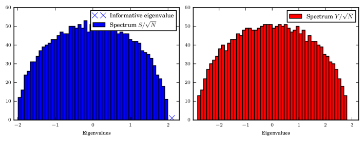
Figure 2: Spectrum of the Fisher score matrix $S/\sqrt{N}$ and of the data matrix $Y/\sqrt{N}$ for the same instance of a problem with exponential output noise in the rank-one symmetric $XX^{\top}$ case. The planted configuration is generated from a Gaussian of zero mean and variance $1.4$. We see that an eigenvalue is out of the bulk for $S$ but not for $Y$. The data were generated on a system of size $N=2000$.

This situation can be quantified using the spectral analysis of section IV.1 applied to two different noise channels $g_{1}(Y,w)=-\beta(\text{ sign}(Y)-w)^{2}/2$ and $g_{2}(Y,w)=-\beta(Y-w)^{2}/4$ and taking the limit $\beta\rightarrow\infty$ as in (171). For these noise channels a theoretical analysis of the top eigenvectors of $S$ and $Y$ can be performed using theory presented in section IV.1. Taking square of (175) and dividing by (176) one can show that the state evolution equation describing the overlap of the top positive eigenvectors of $Y$ and $S$ is given by the only stable fixed point of the following update equation

$$\frac{{(m_{x}^{t+1})}^{2}}{q_{x}^{t+1}}=\frac{\frac{{m_{x}^{t}}^{2}}{q_{x}^{t}}\frac{\sigma^{2}\widetilde{\Delta}}{\widehat{\Delta}^{2}}}{1+\frac{{m_{x}^{t}}^{2}}{q_{x}^{t}}\frac{\sigma\widetilde{\Delta}}{\widehat{\Delta}^{2}}}\,,$$ (188)

$$\widehat{\Delta}=\widetilde{\Delta}=1:{\rm for}\,g_{1}(Y,w)\,,$$ (189)

$$\widehat{\Delta}=\widetilde{\Delta}=2:{\rm for}\,g_{2}(Y,w)\,,$$ (190)

where $\widehat{\Delta}$ and $\widetilde{\Delta}$ are computed when $\beta=1$. The trivial fixed point $\frac{{m_{x}^{t}}^{2}}{q_{x}^{t}}=0$ of this equation is unstable as soon as

$$\sigma^{2}\geq\frac{\widehat{\Delta}^{2}}{\widetilde{\Delta}}\,.$$ (191)

This analysis tells us that the top eigenvectors are correlated with the planted solution $x^{0}$ when $\sigma>1$ for $S$ and $\sigma>2$ for $Y$. Therefor for $\sigma=1.4$ the Fisher score matrix has informative leading eigenvector, while the top eigenvector of $Y$ does not contain any information on the planted solution.

IV.2.3 Stability of the uniform fixed point in Bayes-optimal setting

In this section we restrict for simplicity to the Bayes optimal setting defined by eq. (7). As we derived in section III the evolution of the Low-RAMP algorithm can be tracked using the state evolution equations. In the Bayes optimal case we have $\overline{R}=0$ therefore the (sufficient) condition for the existence of the uniform fixed point is to have prior $P_{X}$ (or both $P_{U}$ and $P_{V}$) of zero mean. The existence of a uniform fixed point of the Low-RAMP algorithm translates into the existence of a fixed point of the state evolution with $M^{t}_{x}=0$ for the symmetric case (or $M^{t}_{u}=M^{t}_{v}=0$ for the bipartite case).

The stability of this fixed point is analyzed by expanding in linear order the state evolution equation (151) around the uniform fixed point, taking into account the definition of the thresholding function (56). For the $XX^{\top}$ case this gives

$$M_{x}^{t+1}=\frac{\Sigma_{x}M_{x}^{t}\Sigma_{x}}{\Delta}\,,$$ (192)

where $\Sigma_{x}$ in the Bayes-optimal case is the covariance matrix of the signal (and prior) distribution as given by eq. (150). Calling $\lambda^{x}_{\rm max}$ the largest eigenvalue of the covariance of the distribution of the signal-elements, $\Sigma_{x}$, we obtain a simple criterion for the stability of the uniform fixed point

$$\left\{\begin{matrix}\Delta_{c}=(\lambda^{x}_{\rm max})^{2}<\Delta\Rightarrow{\rm stable}\\ \Delta<\Delta_{c}=(\lambda^{x}_{\rm max})^{2}\Rightarrow{\rm unstable}\end{matrix}\right.\,.$$ (193)

It is useful to specify that for the rank-one case where both $\Sigma_{x}$ and $M_{x}$ are scalars we get $\Sigma_{x}=\langle x^{2}_{0}\rangle$ to be the variance of the prior distribution $P_{x}$. For the rank one, $r=1$, case the stability criterium becomes

$$\left\{\begin{matrix}\Delta_{c}=\langle x^{2}_{0}\rangle^{2}<\Delta\Rightarrow{\rm stable}\\ \Delta<\Delta_{c}=\langle x^{2}_{0}\rangle^{2}\Rightarrow{\rm unstable}\end{matrix}\right.\,.$$ (194)

Interestingly, the criteria (193) is the same as the criteria for the spectral phase transition of the Fisher score matrix $S$. When the uniform fixed point is not stable the Fisher score matrix has an eigenvalue going out of the bulk baik2005phase ; hoyle2004principal . We stress here that this analysis is particular to signals of zero mean. If the mean is non-zero the spectral threshold does not change, but the Bayes optimal performance gets better and hence superior to PCA.

The critical value of $\Delta_{c}$ separates two parts of the phase diagram

• For $\Delta>\Delta_{c}$ inference is algorithmically hard or impossible. The Low-RAMP algorithm (and sometimes it is conjectured that all other polynomial algorithms) will not be able to get a better MSE than corresponding to random guessing from the prior distribution.

• For $\Delta<\Delta_{c}$ inference better than random guessing is algorithmically efficiently tractable. The Low-RAMP and also PCA give an MSE strictly better that random guessing from the prior.

For the bipartite case, $UV^{\top}$, the stability analysis is a tiny bit more complicated since there are two order parameters $M_{u}^{t}$ and $M_{v}^{t}$. Linearization of the state evolutions leads to

$$M_{u}^{t} = \alpha\frac{\Sigma_{u}M_{v}^{t}\Sigma_{u}}{\Delta}\,,$$ (195)

$$M_{v}^{t+1} = \frac{\Sigma_{v}M_{u}^{t}\Sigma_{v}}{\Delta}\,,$$ (196)

where in the Bayes-optimal case the $\Sigma_{u}$ and $\Sigma_{v}$ are simply the covariances of the prior distribution $P_{U}$ and $P_{V}$, i.e. $\Sigma_{u}=\langle uu^{\top}\rangle$ and $\Sigma_{v}=\langle vv^{\top}\rangle$. By replacing (196) in (195) one gets

$$M_{u}^{t+1}=\left(\frac{\sqrt{\alpha}{\Sigma_{u}{\Sigma_{v}}}}{\Delta}\right)M_{u}^{t}\left(\frac{\sqrt{\alpha}{\Sigma_{u}{\Sigma_{v}}}}{\Delta}\right)^{\top}\,.$$ (197)

Calling $\lambda_{\rm max}^{uv}$ the largest eigenvalue of the matrix $\Sigma_{u}{\Sigma_{v}}$ gives us the stability criteria of the uniform fixed point in the bipartite case as

$$\left\{\begin{matrix}\Delta_{c}=\sqrt{\alpha}\lambda_{\rm max}^{uv}<\Delta\Rightarrow{\rm Stable}\\ \Delta<\Delta_{c}=\sqrt{\alpha}\lambda_{\rm max}^{uv}\Rightarrow{\rm Unstable}\end{matrix}\right.\,.$$ (198)

Also this criteria agrees with the criteria for spectral phase transition for the Fisher score matrix and also here $\Delta_{c}$ separates two parts of the phase diagram, one where estimating the signal betten than randomly sampling from the prior distribution is not posible with Low-RAMP (and conjecturally with no other polynomial algorithm), and another where the MSE provided by Low-RAMP or PCA is strictly better than the one achieved by guessing at random.

IV.3 Multiple stable fixed points: First order phase transitions

The narrative of this paper is to transform the high-dimensional problem of low-rank matrix factorization to analysis of stable fixed point of the Low-RAMP algorithms and correspondingly of the state evolution equations. A case that deserves detailed discussion is when there exists more than one stable fixed point. The present section is devoted to this discussion in the Bayes-optimal setting, where the replica symmetric assumption is fully justified and hence a complete picture can be obtained.

We encounter two types of situations with multiple stable fixed points

• Equivalent fixed points due to symmetry: The less interesting type of multiple fixed points arises when there is an underlying symmetry in the definition of the problem, then both the state evolution and and Low-RAMP equations have multiple fixed points equivalent under the symmetry. All these fixed points have the same Bethe and replica free energy. One example of such a symmetry is a Gaussian prior of zero mean and isotropic covariance matrix. Then there is a global rotational symmetry present. Another example of a symmetry is given by the community detection problem defined in section I.4.2. In the case of $r$ symmetric equally sized groups with connectivity matrix (37) there is a permutational symmetry between communities so that any fixed of the state evolution or Low-RAMP equations exists in $r!$ versions.

• Non-equivalent fixed points. More interesting case is when Low-RAMP and the state evolution equations have multiple stable fixed points, not related via any symmetry, having in general different free-energies. This is then related to phenomenon that is in physics called the first order phase transition. This is the type that we will discuss in detail in the present section.

In general, it is the fixed point with highest free energy that provides the true marginals of the posterior distribution (we remind change of sign in our definition of the free energy w.r.t. the standard physics definition). From an algorithmic perspective, it is the fixed point achieved from uninformed initialization (see below) that gives a way to compute the error achievable by the Low-RAMP algorithm. A conjecture that appears in a number of papers analyzing Bayes optimal inference on random instances is that the error reached by Low-RAMP is the best achievable with a polynomial algorithm. Note, however, that replica symmetry breaking effects might play a role out of the equilibrium solution and hence may influence the properties of the best achievable mean-squared-error.

IV.3.1 Typical first order phase transition: Algorithmic interpretation

The concept of a first order phase transition is best explained on a specific example. For the sake of the explanation we will consider the symmetric $XX^{\top}$ case in the Bayes optimal setting. For the purpose of giving a specific example we consider the Gaussian output channel with variance of the noise $\Delta$, the signal is drawn from the spiked (i.e. $r=1$) Rademacher-Bernoulli model with fraction of non-zeros being $\rho=0.08$.

In Fig. 3 we plot all the fixed points of the state evolution equation and the corresponding value of the replica free energy (153) as a function of $\Delta/\rho^{2}$. The equations for the state evolution specific to the spiked Rademacher-Bernoulli model are given by (214). For this model the uniform fixed point exists and is stable down to $\Delta_{c}=\rho^{2}$, eq. (193). The numerically stable fixed points are drawn in blue, the unstable ones in red. We focus on the interval of $\Delta$ where more than one stable fixed point of the state evolution (151) exists. We use the example of the spiked Rademacher-Bernoulli model for the purpose of being specific in figure 3. The definitions and properties defined in the rest of this section are generic and apply to all the settings considered in this paper, not only to the spiked Rademacher-Bernoulli model.

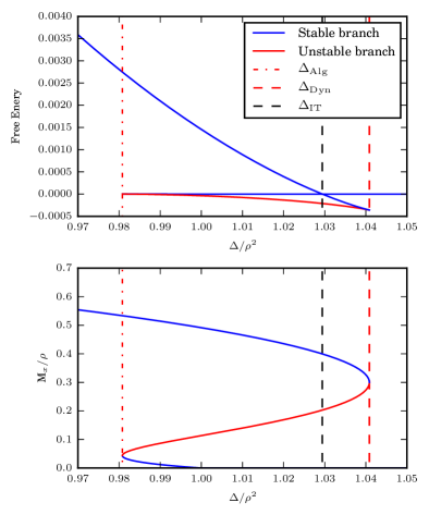
Figure 3: In the lower pannel, we plot as a function of $\Delta/\rho^{2}$ all the fixed points $M_{x}/\rho$ of state evolution equations (151) for the spiked Rademacher-Bernoulli model with fraction of non-zero being $\rho=0.08$. Numerically stable fixed points are in blue, unstable in red. We remind that the order parameter $M_{x}$ is related to the mean-squared error as ${\rm MSE}_{X}={\rm Tr}\left[\langle x_{0}x_{0}^{\top}\rangle-M_{x}\right]$. In the upper pannel, we plot the replica free energy (153) corresponding to these fixed points, again as a function of $\Delta/\rho^{2}$. When there are multiple stable fixed points to the SE equations the one that corresponds to performance of the Bayes optimal estimation is the one with the largest free energy (we remind that with respect to the most common physics notation we defined the free energy as the positive logarithm of the partition function). The $\Delta$ for which these two branches cross in free-energy is called the information theoretic phase transition, $\Delta_{\rm IT}$. The two spinodal transitions $\Delta_{\rm Alg}$ and $\Delta_{\rm Dyn}$ are where the lower MSE an higher MSE stable fixed point disappears. The $\Delta_{c}/\rho^{2}=1$ corresponds to the spectral transition at which the uniform fixed point become unstable.

Let us define two (possibly equal) stable fixed points of the state evolution as follows:

• $M_{\rm Uninformative}(\Delta)$ is the fixed point of the state evolution one reaches when initialising the $M^{t=0}=\epsilon I_{r}$ (with $\epsilon$ very small and positive, $I_{r}$ being the identity matrix). We call this the uninformative initialisation.

• $M_{\rm Informative}(\Delta)$ is the fixed point of the state evolution one reaches when initialising the $M^{t=0}=\langle xx^{\top}\rangle$. This is the informative initialisation where we start as if the planted configuration was known.

In principle there could be other stable fixed points apart of $M_{\rm Uninformative}(\Delta)$ and $M_{\rm Informative}(\Delta)$, but among all the examples that we analyzed in this paper we have not observed any such case. In this paper we hence discuss only the case with at most two stable fixed points, keeping in mind that if more stable fixed points exist than the theory does apply straightforwardly as well (the physical fixed point is still the one of highest free energy), and there could be several first order phase transitions following each other as $\Delta$ is changed.

With two different stable fixed points existing for some values of $\Delta$ we observe three critical values defined as follows

• $\Delta_{\rm Alg}$ called the algorithmic spinodal transition, is the value of $\Delta$ at which the fixed point $M_{\rm Uninformative}$ stops existing and becomes equal to $M_{\rm Informative}$.

• $\Delta_{\rm IT}$ called the information theoretic phase transition, is the value of $\Delta$ at which the two fixed points $M_{\rm Uninformative}\neq M_{\rm Informative}$ exist and have the same replica free energy (153).

• $\Delta_{\rm Dyn}$ called the dynamic spinodal transition, is the value of $\Delta$ at which the fixed point $M_{\rm Informative}$ stops existing and becomes equal to $M_{\rm Uninformative}$.

In Fig. 3 these three transition are marked by vertical dashed lines, the information theoretic transition in black and the two spinodal transition in red.

We recall that for the priors of zero mean, where the uniform fixed points discussed in section IV.2.1 exists, the stability point of the uniform fixed point $\Delta_{c}$ (193) is in general unrelated to the $\Delta_{\rm Alg}$, $\Delta_{\rm IT}$ and $\Delta_{\rm Dyn}$. In the example presented in Fig. 3 of spiked Rademacher-Bernoulli model at $\rho=0.08$ we have $\Delta_{\rm Alg}<\Delta_{c}<\Delta_{\rm IT}$. In general the position of $\Delta_{c}$ with respect to $\Delta_{\rm Alg}$, $\Delta_{\rm IT}$ and $\Delta_{\rm Dyn}$ can be arbitrary, in the following sections we will observe several examples. A notable situation is when $\Delta_{c}=\Delta_{\rm Alg}$, cases where this happen are discussed in section IV.3.3. It should be noted that this is the case in the community detection problem, and since this is a well known and studied example it is sometimes presented in the literature as the generic case. But from the numerous examples presented in this paper we see that cases where $\Delta_{c}\neq\Delta_{\rm Alg}$ are also very common.

Phase transitions are loved and cherished in physics, in the context of statistical inference the most intriguing properties related to phase transitions is their implications in terms of average computational complexity. Notably in the setting of Bayes-optimal low-rank matrix factorization as studied in this paper we distinguish two different regions

• Phase where Low-RAMP is asymptotically Bayes-optimal: For $\Delta\geq\Delta_{\rm IT}$ and for $\Delta\leq\Delta_{\rm Alg}$ the Low-RAMP algorithm in the limit of large system sizes gives the information theoretically optimal performance. This is either because the fixed point it reaches is unique (up to symmetries) or because it is the one with larger free energy.

• The hard phase: For $\Delta_{\rm Alg}<\Delta<\Delta_{\rm IT}$ the estimation error achieved by the Low-RAMP algorithm is strictly larger that the lowest information-theoretically achievable error. On the other hand, and in line with other statistical physics works on inference problems in the Bayes optimal setting, we conjecture that in this region no other polynomial algorithm that would achieve better error than Low-RAMP exists. This conjecture could be slightly modified by the fact that the branch of stable fixed points that do not correspond to the MMSE could present aspects of replica symmetry breaking which could modify its position. Investigation of this is left for future work.

From a mathematically rigorous point of view the results of this paper divide into three parts:

• (a) Those that are rigorous, known from existing literature that is not related to statistical physics considerations. An example is given by the performance of the spectral methods that is better that random guessing for $\Delta<\Delta_{c}$ baik2005phase .

• (b) A second part regroups the results directly following from the analysis of the Bayes-optimal Low-RAMP and the MMSE that are not presented rigorously in this paper, but were made rigorous in a series of recent works krzakala2016mutual ; barbier2016mutual ; LelargeMiolane16 ; miolane2017fundamental . Most of these results are proven and although some cases are still missing a rigorous proof, it is safe to assume that it is a question of time that researchers will fill the corresponding gaps and weaken the corresponding assumptions. For instance the state evolution of Low-RAMP rangan2012iterative ; javanmard2013state ; DeshpandeM14 , its Bayes-Optimality in the easy phase (at least for problem where the paramagnetic fixed point is not symmetric) and the value of the information theoretically optimal MMSE krzakala2016mutual ; deshpande2016asymptotic ; barbier2016mutual ; LelargeMiolane16 ; miolane2017fundamental are all proven rigorously.

• (c) The third kind of claims are purely conjectures. For instance, the claim that among all polynomial algorithms the performance of Low-RAMP cannot be improved (so that the hard phase is indeed hard). Of course proving this in full generality would imply that P$\neq$NP and so we cannot expect that such a proof would be easy to find. At the same time from a broad perspective of understanding average computational complexity this is the most intriguing claim and is worth detailed investigation and constant aim to find a counter-example.

IV.3.2 Note about computation of the first order phase transitions

In this section we discuss how to solve efficiently the SE equations in the $XX^{\top}$ Bayes optimal case for rank one. We notice that for a given prior distribution $P_{X}$ the only way the symmetric Bayes optimal state evolution, eq.  (151), depends on the noise parameter $\Delta$ is via the ratio $m^{t}/\Delta$. One can write the SE equations in the form (152)

$$m^{t+1}=f_{P_{X}}^{\rm SE}\left(\frac{m^{t}}{\Delta}\right)\,.$$ (199)

Let us further define fixed points of (199) in a parametric way

$$\Delta=\frac{f_{P_{X}}^{\rm SE}(x)}{x}\,,$$ (200)

$$m=f_{P_{X}}^{\rm SE}(x)\,.$$ (201)

To get a fixed point $(m,\Delta)$ of (199) we choose a value of $x$ and compute $(f(x),f(x)/x)$. We observe from the form of the state evolution (rank-one symmetric Bayes optimal case) that $f(x)$ is a non-decreasing function of $x$. We further observe that $(m,\Delta)$ is a stable fixed points if and only if $\partial_{x}\Delta(x)<0$. The two spinodal thresholds $\Delta_{\rm Alg}$ and $\Delta_{\rm Dyn}$ are defined by loss of existence of corresponding stable fixed points and they can hence be computed as

$$\Delta_{\rm Alg},\Delta_{\rm Dyn}\in\left\{\Delta(x),x\in\mathbb{R}^{+},\frac{\partial\Delta(x)}{\partial x}=0\right\}\,.$$ (202)

The information theoretic transition $\Delta_{\rm IT}$ relies on computation of the replica free energy (153). Using the fact that

$$\frac{\partial\phi(m,\Delta)}{\partial m}=\frac{1}{2\Delta}\left(f_{P_{X}}^{\rm SE}\left(\frac{m}{\Delta}\right)-m\right)$$ (203)

allows us to compute the difference in energy between a fixed point $m,\Delta$ and the uniform fixed point $m=0$ as

$$\phi(m(x),\Delta(x))-\phi(0,\Delta(x))=\frac{1}{2}\left[\int_{0}^{x}{\rm d}u\,f_{P_{X}}^{\rm SE}(u)-\frac{xf^{\rm SE}(x)}{2}\right]\,.$$ (204)

The $x_{\rm IT}$ for which (204) is zero then gives the information theoretic phase transition $\Delta_{\rm IT}=f(x_{\rm IT})/x_{\rm IT}$.

IV.3.3 Sufficient criterium for existence of the hard phase

This section is specific to the Bayes-optimal cases when the prior $P_{X}$ has a zero mean and hence the uniform fixed point of the Low-RAMP and the state evolution exists. In section IV.2.3 we derived that the uniform fixed point is stable at $\Delta>\Delta_{c}$ and unstable for $\Delta<\Delta_{c}$. It follows from the theory of bifurcations that the critical point where a fixed-point changes stability must be associated with an onset of another close-by fixed point. In general there are two possibilities

• 2nd order bifurcation. If the fixed point close to the uniform fixed point departs in the direction of smaller $\Delta<\Delta_{c}$, where the uniform fixed point is unstable, then this close-by fixed point is stable. This case corresponds to Fig. 3. Behaviour in the vicinity of the uniform fixed point then does not let us distinguish between (a) existence of a first order phase transition at lower $\Delta$ (as in Fig. 3), or (b) continuity on the MMSE down to $\Delta=0$ with no algorithmically hard phase existing in that case.

• 1st order bifurcation. If the fixed point close to the uniform fixed point departs in the direction of larger $\Delta>\Delta_{c}$, where the uniform fixed point is stable, then this close-by fixed point is unstable. In that case, the fixed point that is stable from $\Delta<\Delta_{c}$ is not close to the uniform fixed point and this case forces existence of a first order phase transition with $\Delta_{c}=\Delta_{\rm Alg}$.

Expansion of the state evolution (151) around the uniform fixed point gives us a closed form criteria to distinguish whether the phase transition happening at $\Delta_{c}$ is a 1st or 2nd order bifurcation. In case of a 2nd order bifurcation, this expansion allows us to compute the mean squared error obtained with Low-RAMP close to $\Delta_{c}$.

For specificity we consider the rank-one, $r=1$ case, and expand eq. (151) to 2nd order to get

$$m^{t+1}=m^{t}\frac{\langle x_{0}^{2}\rangle^{2}}{\Delta}-\frac{(m^{t})^{2}}{\Delta^{2}}\left(\langle x_{0}^{2}\rangle^{3}-\frac{{\langle x_{0}^{3}\rangle}^{2}}{2}\right)+O\left((m^{t})^{3}\right)\,,$$ (205)

where the mean $\langle\cdots\rangle$ of $x_{0}$ are taken with respect to $P_{X_{0}}=P_{X}$. This is done by expanding $f_{\rm in}^{x}(A,B)$ to order $4$ in $B$ and $2$ in $A$. All the derivatives

$$\forall i,j\quad\frac{\partial^{i+j}f_{\rm in}^{x}}{\partial A^{i}\partial B^{j}}(A=0,B=0)$$ (206)

are linked to moments of the density probability $P_{X}$.

The stability criteria $\Delta_{c}=\langle x_{0}^{2}\rangle^{2}$ appears once again as in section IV.2.3. Below $\Delta<\Delta_{c}$ the uniform fixed point $m=0$ is unstable and $m^{t}$ will converge towards another fixed point different from $m=0$. For $\Delta>\Delta_{c}=\langle x_{0}^{2}\rangle$ the uniform fixed point $m=0$ is stable. Using expansion (205) near $\Delta\simeq\Delta_{c}=\langle x_{0}^{2}\rangle$ we can write what is the other fixed point next to $m_{\rm uniform}=0$, we get

$$m_{\rm close-by}=\frac{\Delta_{c}(\Delta_{c}-\Delta)}{\Delta_{c}^{3/2}-\frac{\langle x_{0}^{3}\rangle^{2}}{2}}+O\left(\left(\Delta-\Delta_{c}\right)^{2}\right)\,.$$ (207)

By definition of the order parameters in the Bayes-optimal setting we must have at a fixed point $m\geq 0$, therefore we distinguish two cases

• If $\langle x_{0}^{3}\rangle^{2}<2\langle x_{0}^{2}\rangle^{3}$, eq. (207) is a stable fixed point in the region $\Delta<\Delta_{c}$. Eq. (207) then gives the expansion of this fixed point. This situation corresponds to Fig. 3 where the Rademacher-Bernoulli prior has zero 3rd moment. This is the 2nd order bifurcation at $\Delta_{c}$.

• $\langle x_{0}^{3}\rangle^{2}>2\langle x_{0}^{2}\rangle^{3}$ eq. (207) is an unstable (and hence irrelevant) fixed point in the region $\Delta>\Delta_{c}$. But also in this case there must be a stable fixed point for $\Delta<\Delta_{c}$, but this fixed point cannot have a small values of $m$. The only way a stable fixed point can appear in this case is by a discontinuous (1st order) transition at $\Delta_{c}$. This is the 1st order bifurcation at $\Delta_{c}$.

To summarize, we obtained a simple (sufficient) criteria for the existence of a first order phase transition with $\Delta_{\rm Alg}=\Delta_{c}$. Notably there is a 1st order phase transition when

$$\left\{\begin{matrix}\langle x_{0}\rangle=0\\ \langle x_{0}^{3}\rangle^{2}>2\langle x_{0}^{2}\rangle^{3}\end{matrix}\right.\,.$$ (208)

The more skewed the prior distribution is the easier the problem is. Till a point where if the skewness of the signal is bigger than $\sqrt{2}$ then a first order phenomena will appear in the system. In this case the MSE achieved by the Low-RAMP algorithm becomes discontinuously better than ${\rm MSE}_{\rm uniform}=\langle x_{0}^{2}\rangle$

On the other hand when the criteria (208) is not met, then for $\Delta<\Delta_{c}$ the MSE achieved by the Low-RAMP algorithm is in first approximation equal to

$${\rm MSE}(\Delta)=\langle x_{0}^{2}\rangle-\frac{\Delta_{c}(\Delta_{c}-\Delta)}{\Delta_{c}^{3/2}-\frac{{\langle x_{0}^{3}\rangle}^{2}}{2}}+O\left(\left(\Delta-\Delta_{c}\right)^{2}\right)\,.$$ (209)

So the MSE obtained by an Low-RAMP algorithm is linear near the transition in $\Delta-\Delta_{c}$.

Interestingly spectral method also give an MSE linear in $\Delta-\Delta_{c}$. As derived in section IV.1 the MSE one achieves using the eigenvectors of matrix $S$ is

$${\rm MSE}_{\rm Spectral}(\Delta)=\langle x_{0}^{2}\rangle-\frac{\Delta_{c}-\Delta}{\sqrt{\Delta_{c}}}\,.$$ (210)

From the coefficient of linearity in the error we observe that the error achieved by PCA is always worse than the error achieved by Low-RAMP.

Let us remind that uniform fixed points and 1st order phase transition (at $\Delta_{\rm Alg}=\Delta_{c}$ or elsewhere) can exist even if the criteria derived above are not met, there are sufficient, not necessary conditions. Examples are included in subsequent sections.

V Phase diagrams for Bayes-optimal low-rank matrix estimation

From now on we restrict our analysis to the Bayes optimal setting as defined in section I.2.1, eq. (7). The motivation is to investigate performance of the Bayes-optimal and the Low-RAMP estimators for a set of benchmark problems. We investigate phase diagrams stemming from the state evolution equations and from the corresponding replica free energies summarized in section III.4.1.

V.1 Examples of phase diagram

In this section we present example of phase diagrams for the symmetric low-rank matrix estimation. The first three examples are for rank one, the last two examples are for general rank.

V.1.1 Spiked Bernoulli model

The spiked Bernoulli model is defined by prior (32) with density $\rho$ of ones, and $1-\rho$ of zeros. This prior has a positive mean and consequently the state evolution does not have the uniform fixed point. This is a problem where one tries to recover a submatrix of size $\rho N\times\rho N$ with mean of elements equal to 1, in a $N\times N$ matrix of lower mean. Using the Bayes-optimal state evolution (126) one gets,

$$m^{t} = f_{\rm Bernoulli}^{\rm SE}\left(\frac{m^{t}}{\Delta}\right)\,,$$ (211)

$$f_{\rm Bernoulli}^{\rm SE}(x) = \rho\mathbb{E}_{W}\left[\frac{\rho}{\rho+(1-\rho)\exp\left(\frac{-x}{2}+W\sqrt{x}\right)}\right]\,,$$ (212)

where $W$ is (here and from now on) a Gaussian variables of zero mean and unit variance.

Depending on the value of $\rho$ there are two kinds of behaviour of the fixed points of these equations as a function of the effective noise $\Delta$. We plot the two cases in Fig. 4. For larger values of $\rho$ there is a unique fixed point corresponding to the MMSE that is asymptotically achieved by the Low-RAMP algorithm, this is the regime in which the proof of DeshpandeM14 applies. For small enough values of $\rho$ we do observe a region of $\Delta_{\rm Alg}<\Delta<\Delta_{\rm Dyn}$ where there are 3 fixed points, two stable and one unstable. The replica free energy associated to the these fixed points crosses at $\Delta_{\rm IT}$ so that the higher fixed point in the relevant one at $\Delta<\Delta_{\rm IT}$, and the lower fixed point at $\Delta>\Delta_{\rm IT}$. These phase transitions were defined in section IV.3.1. In Fig. 5 we plot the phase transitions $\Delta_{\rm Alg}$, $\Delta_{\rm IT}$ and $\Delta_{\rm Dyn}$ as a function of $\rho$. The $y$-axes in the left pannel is simply the effective noise parameter $\Delta$, on the right pannel the same data are plotted with $\Delta/\rho^{2}$ on the $y$-axes. We observe that the $\Delta_{\rm Alg}=_{\rho\to 0}e\rho^{2}$, with $e$ being the Euler number, this is the same asymptotic behaviour as obtained previously in montanari2015finding (Fig. 5).

Figure 4: Plots of the fixed points of the state evolution for the spiked Bernoulli model, MSE being given by ${\rm MSE}=\rho-m$ (154). The performance of PCA as analyzed in section IV.1 is plotted for comparison. These two plots are made for $\rho=0.2$ (left) and $\rho=0.01$ (right).

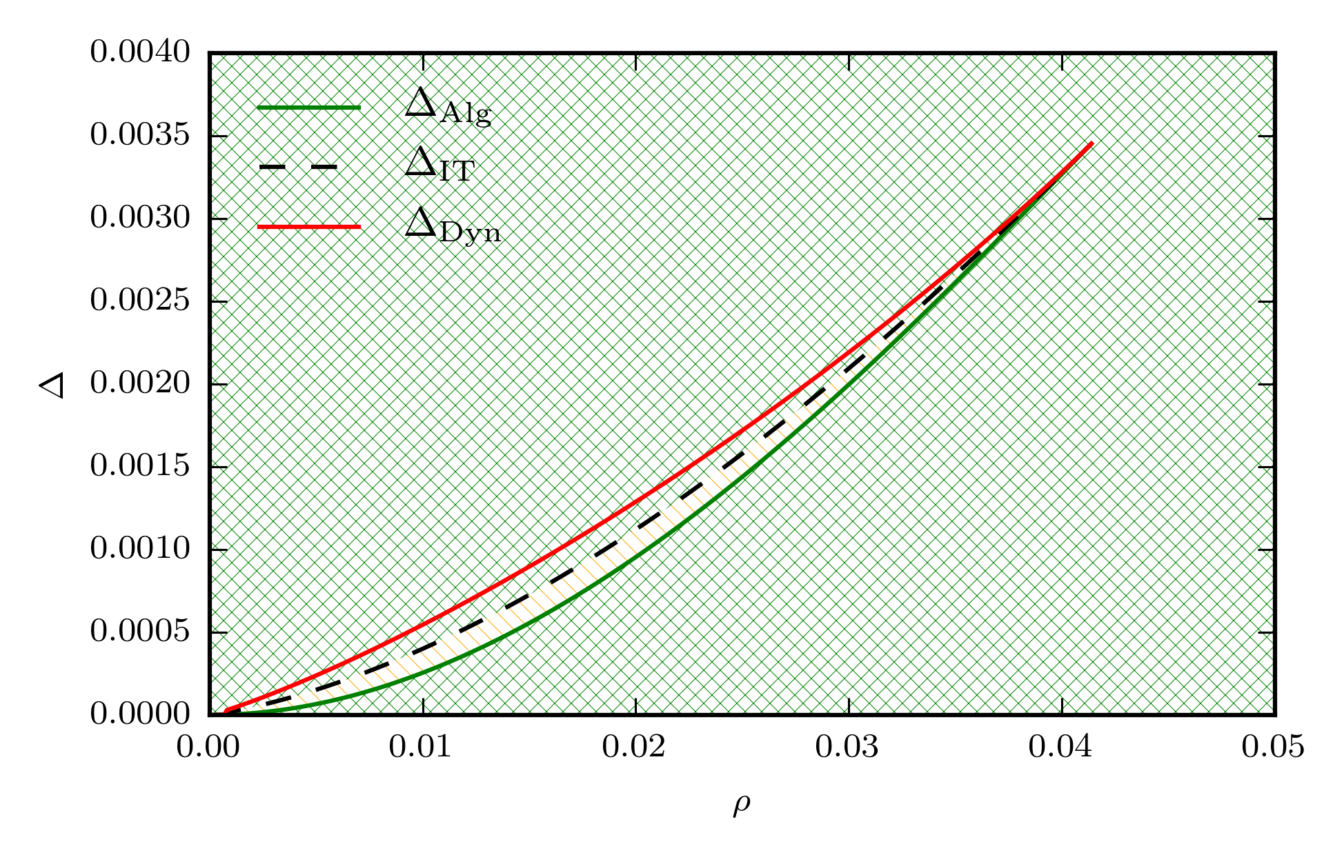
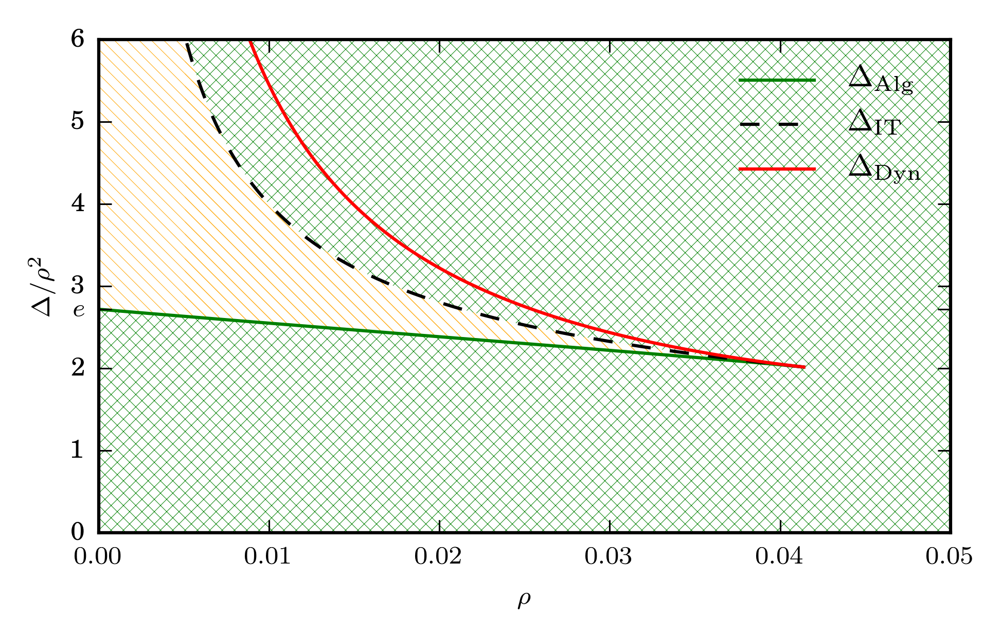
Figure 5: The phase diagram of the spiked Bernoulli model (32) as a function of the density $\rho$ and effective noise $\Delta$ (left) or $\Delta/\rho^{2}$ (right). There is no phase transition in the system for $\rho>0.04139$ and a 1st order phase transition for $\rho<0.04139$. The lower green curve is the algorithmic spinodal $\Delta_{\rm Alg}$ curve, that converges to $\Delta_{\rm Alg}=_{\rho\to 0}e\rho^{2}$. The dashed black line is the information theoretic threshold $\Delta_{\rm IT}$. The upper red curve is the dynamical spinodal $\Delta_{\rm Dyn}$. The orange hashed zone is the hard region in which Low-RAMP does not reach the Bayes-optimal error. In the rest of the phase diagram (green hashed) the Low-RAMP provides in the large size limit the Bayes-optimal error. Note that this is exactly the same phase diagram as presented in montanari2015finding (Fig. 5) for the problem of finding one dense subgraph, this is thanks to output channel universality and the fact that large degree sparse graphs have upon rescaling the same phase diagram as dense graphs.

V.1.2 Rademacher-Bernoulli and Gauss-Bernoulli

Next we analyze the spiked Rademacher-Bernoulli and Gauss-Bernoulli priors defined by (33) and (36). The first thing we notice is that both these distribution have zero mean and variance $\rho$. This means according to (IV.2.1) that there is a uniform fixed point of the SE equations that is stable for $\Delta>\rho^{2}$. The skewness of both these distribution is 0, which means that at $\Delta_{c}$ there is no discontinuity of the $\rm MSE$ (IV.3.3). The SE equations for these models are

$$m^{t+1} = f_{\rm Rademacher-Bernoulli}^{\rm SE}\left(\frac{m^{t}}{\Delta}\right)\,,$$ (213)

$$f_{\rm Rademacher-Bernoulli}^{\rm SE}(x) = \rho\mathbb{E}_{W}\left[\tanh\left(x+W\sqrt{x}\right)\frac{\rho}{(1-\rho)\frac{\exp(x/2)}{\cosh\left(x+W\sqrt{x}\right)}+\rho}\right],$$ (214)

$$m^{t+1} = f_{\rm Gaussian-Bernoulli}^{\rm SE}\left(\frac{m^{t}}{\Delta}\right)\,,$$ (215)

$$f_{\rm Gauss-Bernoulli}^{\rm SE}(x)/\rho = \frac{x}{1+x}\mathbb{E}_{W}\left[W^{2}\hat{\rho}(x,W\sqrt{x^{2}+x})\right],$$ (216)

where $\hat{\rho}$ is

$${\hat{\rho}}(a,b^{2})=\frac{\rho}{(1-\rho)\exp\left(\frac{-b^{2}}{2(1+a)}\right)(1+a)^{\frac{r}{2}}+\rho}\,.$$ (217)

Both these models have similar phase diagram.

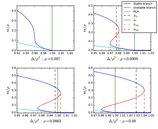
Figure 6: We plot all the fixed points of the state evolution equations for the spiked Rademacher-Bernoulli model in the Bayes optimal setting as a function of ${\Delta/\rho^{2}}$ for four representative values of $\rho$. The blue curves are stable fixed points, red are the unstable ones. MSE is given by (154). The vertical lines mark the two spinodal transition (dynamical $\Delta_{\rm Dyn}$ and algorithmic $\Delta_{\rm Alg}$, red dashed), the information theoretic transition $\Delta_{\rm IT}$. The vertical green full line mark the stability point of the uniform fixed point $\Delta_{c}=\rho^{2}$. We remind that the error ${\rm MSE}=\rho-m$ achieved by the Bayes optimal estimator corresponds to the upper branch for $\Delta<\Delta_{\rm IT}$, and to the lower branch for $\Delta>\Delta_{\rm IT}$. Error achieved by the Low-RAMP algorithm always correspond to the lower branch (larger error). Note that in the three panels where multiple fixed points exists, the only element that changes is the position of the (spectral) stability threshold $\Delta_{c}$ with respect to the other thresholds.

We first illustrate in Fig. 6 the different types of phase transition that we observe for the spiked Rademacher-Bernoulli model as the density $\rho$ is varied. We plot all the fixed points of equation (214) for several values of $\rho$ as a function of the effective noise $\Delta/\rho^{2}$. The four observed case are the following

• $\rho=0.097$ example: For $\rho$ large enough (in the present case $\rho>\rho_{\rm tri}=0.0964$) whatever the $\Delta$ there is only one stable fixed point.

• For small enough $\rho<\rho_{\rm tri}=0.0964$ three different fixed points exist in a range of $\Delta_{\rm Alg}(\rho)<\Delta<\Delta_{\rm Dyn}(\rho)$, where the thresholds $\Delta_{\rm Alg}$, and $\Delta_{\rm Dyn}$ are defined by the limits of existence of the three fixed points. The information theoretic threshold where the free energy corresponding to the two stable fixed points crosses is $\Delta_{\rm IT}$. Depending on the values of $\rho$ we observed 3 possible scenarios of how $\Delta_{c}=\rho^{2}$ is placed w.r.t. the other thresholds.

  • $\rho=0.0909$ example where $\Delta_{\rm Dyn}<\Delta_{c}$.

  • $\rho=0.0863$ example where $\Delta_{\rm IT}<\Delta_{c}<\Delta_{\rm Dyn}$.

  • $\rho=0.08$ examples where $\Delta_{\rm Alg}<\Delta_{c}<\Delta_{\rm IT}$.

Finally Fig. 8 presents the four thresholds $\Delta_{\rm Dyn}$, $\Delta_{\rm IT}$, $\Delta_{\rm Alg}$ and $\Delta_{c}$ as a function of the density $\rho$.

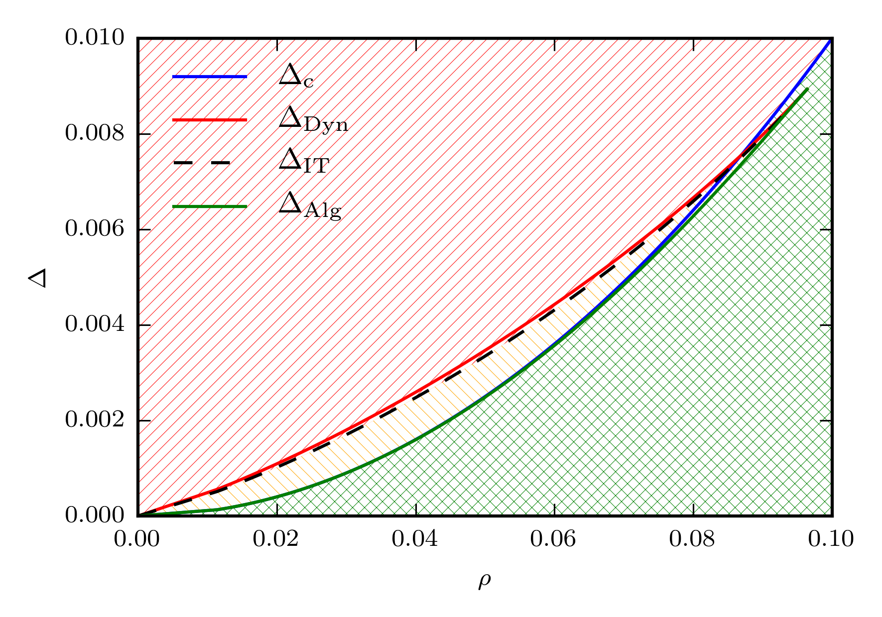
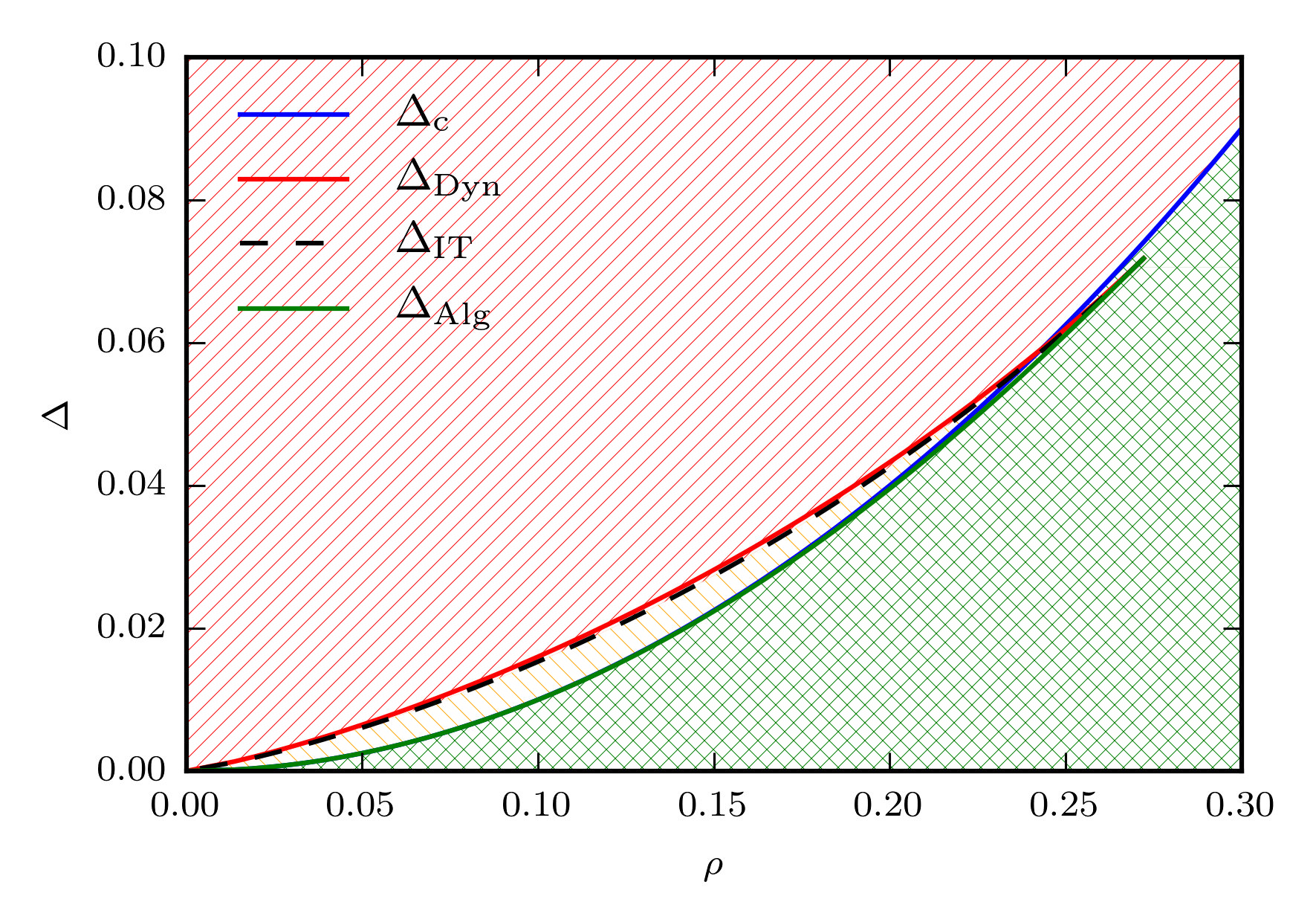
Figure 7: Phase diagram of the spiked Rademacher-Bernoulli (left hand side pannel) and spiked Gauss-Bernoulli (right hand side pannel) models. We plot $\Delta$ as a function of $\rho$. The local stability threshold of the uniform fixed point $\Delta_{c}/\rho^{2}=1$ is in blue. The algorithmic spinodal $\Delta_{\rm Alg}$ (green), the dynamical spinodal $\Delta_{\rm Dyn}$ (red) and the information theoretic transition $\Delta_{\rm IT}$ (black dashed) all join into a tri-critical point located at $(\Delta_{\rm tri}=0.008935,\Delta_{\rm tri}/\rho_{\rm tri}^{2}=0.9612,\rho_{\rm tri}=0.09641)$ for the Rademacher-Bernoulli model (left pannel), and at $(\Delta_{\rm tri}=0.07182,\Delta_{\rm tri}/\rho_{\rm tri}^{2}=0.9693,\rho_{\rm tri}=0.2722)$ for the Gauss-Bernoulli model (right pannel). The hash materializes the different phases. The easy phase where the Low-RAMP algorithm is Bayes-optimal and achieves better error than random guessing is hashed in green crossed lines, the hard phase where Low-RAMP is suboptimal is hashed in yellow $\setminus\setminus$, and the impossible phase where even the best achievable error is as bad as random guessing is hashed in red $//$.

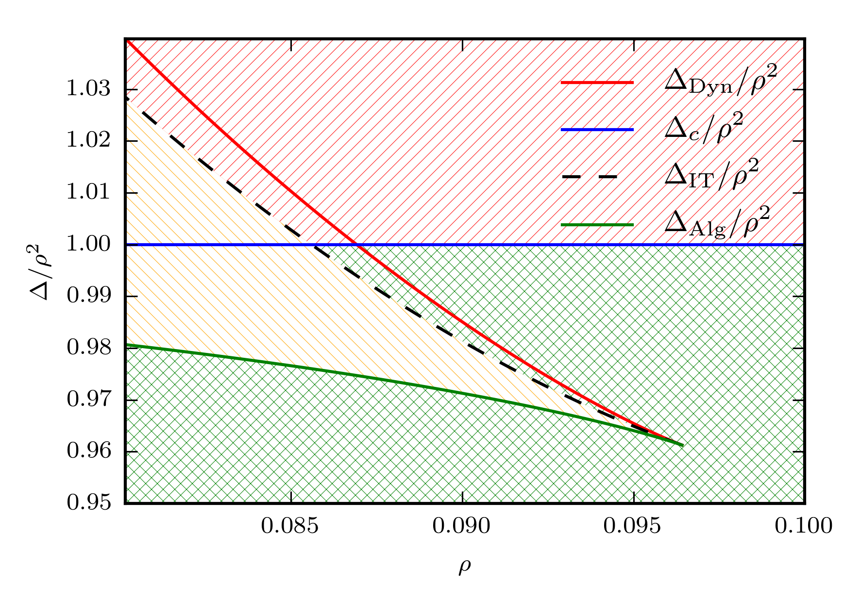
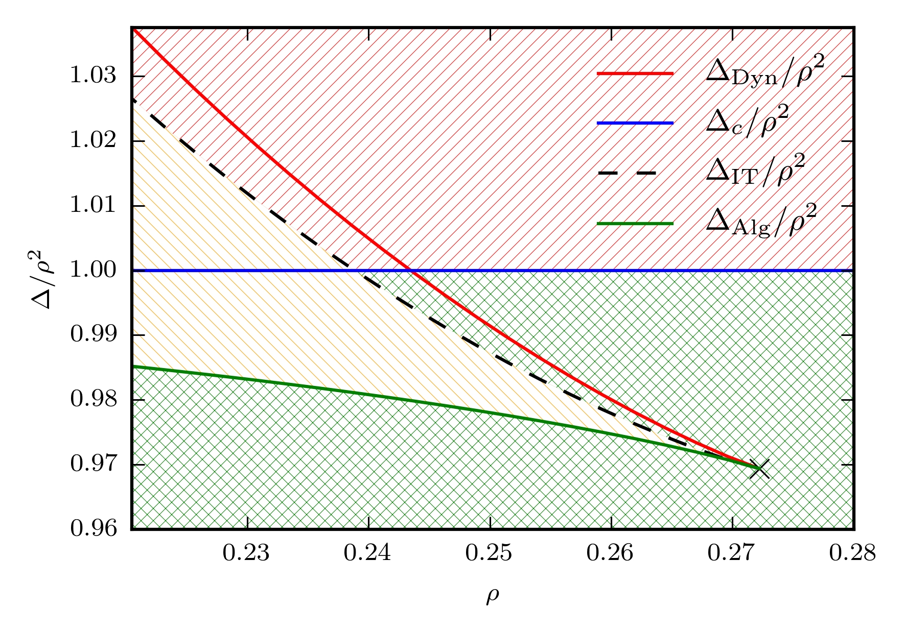
Figure 8: The same plot as in Fig. 7 zoomed into the region of the tri-critical point with $y$-axes rescaled by $\rho^{2}$. The spiked Rademacher-Bernoulli mode on left hand side pannel, the spiked Gauss-Bernoulli model on the right hand side.

In Fig. 9 we present for completness the comparison between the fixed points on the state evolution and the fixed points of the Low-RAMP algorithm for the Gauss-Bernoulli model, with rank one, Bayes optimal case. The experiment is done on one random instance of size $N=2\times 10^{4}$ and we see the agreement is very good, finite size effect are not very considerable. The data are for the Gauss-Bernoulli model at $\rho=0.1$, that is in a region where $\Delta_{\rm Alg}$ is so close to $\Delta_{c}$ that in this figure the difference is unnoticeable.

We also compare to the MSE reached by the PCA spectral algorithm and from its analysis eq. (183). We see that whereas both Low-RAMP and PCA work better than random guesses below $\Delta_{c}$, the MSE reached by Low-RAMP is considerably smaller.

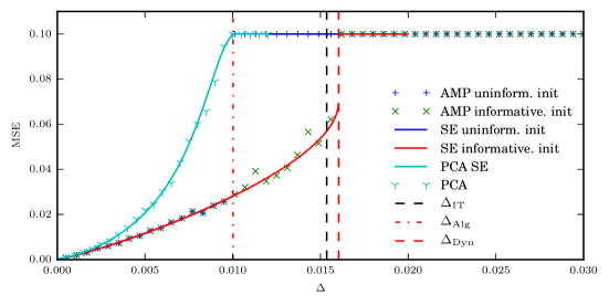
Figure 9: Comparison between the state evolution and the fixed point of the Low-RAMP algorithm, for the spiked Gauss-Bernoulli model of sparse PCA with rank one and density $\rho=0.1$. The phase transitions stemming from state evolution are $\Delta_{\rm Alg}\approx\Delta_{\rm c}=0.01,\Delta_{\rm IT}=0.0153,\Delta_{\rm Dyn}=0.0161$. The points are the fixed points of the Low-RAMP algorithm run on one typical instance of the problem of size $N=20000$. Blue pluses is the MSE reached from an uninformative initialization of the algorithm. Green crosses is the MSE reached from the informative initialization of the algorithm.

V.1.3 Two balanced groups

The next example of phase diagram we present is for community detection with two balanced (i.e. one group is smaller $\rho N$, but both have the same average degree) groups as defined in eqs. (45-46). This is an example of a system where the bifurcation at $\Delta_{c}$ is of a first order, with $\Delta_{c}=\Delta_{\rm Alg}$. In this problem the prior given by eq. (46), with $\langle x_{0}\rangle=0$, $\langle(x_{0})^{2}\rangle=1$. The output channel is of the stochastic block model type eq. (41-42), leading to effective noise parameter

$$\Delta=\frac{p_{\rm out}(1-p_{\rm out})}{\mu^{2}}\,,$$ (218)

where $\mu$ and $p_{\rm out}$ are the parameters from (41-42). Therefore the uniform fixed point becomes unstable when $\Delta<1$.

Using eqs. (126) and (46) we get for the state evolution for community detection with two balanced groups

$$m^{t+1}=f_{\rm TwoBalanced}^{\rm SE}\left(\frac{m^{t}}{\Delta}\right),\forall t,m^{t}\in[0;1]\,,$$ (219)

where

$$f_{\rm TwoBalanced}^{\rm SE}(x)=\int\limits_{-\infty}^{+\infty}\frac{e^{\frac{-u^{2}}{2}}}{\sqrt{2\pi}}\frac{2\rho(1-\rho)\sinh\left(\frac{x}{2\rho(1-\rho)}+u\sqrt{\frac{x}{\rho(1-\rho)}}\right)}{1+2\rho(1-\rho)\left(\cosh\left(\frac{x}{2\rho(1-\rho)}+u\sqrt{\frac{x}{\rho(1-\rho)}}\right)-1\right)}\,.$$ (220)

To investigate whether $\Delta_{c}=1$ is a 1st or 2nd order bifurcation we compute the second order expansion of the state evolution equations as we have done in (205). We find that the expansion of the state evolution up to second order for the two balanced communities is

$$m^{t+1}=f_{\rho}\left(\frac{m^{t}}{\Delta}\right)=\frac{m^{t}}{\Delta}+\left(\frac{m^{t}}{\Delta}\right)^{2}\frac{1-6\rho(1-\rho)}{2\rho(1-\rho)}\,.$$ (221)

In a similar fashion as in section (IV.3.3) it is the sign of the second order terms that decides between 1st or 2nd order bifurcation at $\Delta_{c}=1$. We find that if $\rho(1-\rho)<1/6$ then the second order derivative of (220) is positive leading to a jump in MSE when $\Delta$ crosses the value $\Delta=1$ which means that there will be first order phase transition for all

$$\rho\in\left[0;\frac{1}{2}-\frac{1}{\sqrt{12}}\approx 0.21\right]\cup\left[\frac{1}{2}+\frac{1}{\sqrt{12}}\approx 0.89;1\right]\,.$$ (222)

It turns out that for the two balanced groups this criteria is both sufficient and necessary. Out of the interval (222) the phase transition at $\Delta_{c}$ is of second order, with no discontinuities. Defining the phase transitions $\Delta_{\rm Alg}$, $\Delta_{\rm IT}$, $\Delta_{\rm Dyn}$ as before in section IV.3.1, we have $\Delta_{\rm Alg}=\Delta_{c}$ and we plot the three phase transitions for community detection for two balanced groups in the phase diagram Fig. 10.

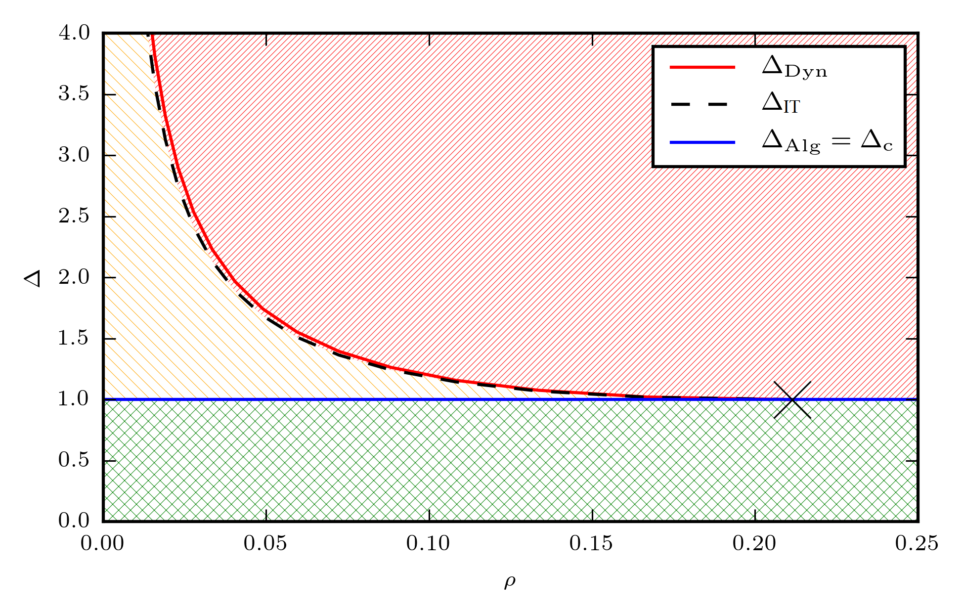
Figure 10: We plot here $\Delta_{\rm Alg}=\Delta_{c}$, $\Delta_{\rm IT}$ and $\Delta_{\rm Dyn}$ as a function of $\rho$ for the community detection with two balanced groups. All the curves merge at $\rho=\frac{1}{2}-\frac{1}{\sqrt{12}}$. The hashed regions have the same meaning as in previous figures, red is the impossible inference phase, green is easy and yellow is hard inference.

V.1.4 Jointly-sparse PCA generic rank

In this section we discuss analysis of the Gauss-Bernoulli jointly sparse PCA as defined by the prior distribution (35) for a generic rank $r$. This just means that each vector $x_{i}\in{\mathbb{R}}^{r}$ is either $\vec{0}$ with probability $1-\rho$ or is taken from Gaussian density probability of mean zero and covariance matrix $I_{r}$ with probability $\rho$. The prior distribution (35) has a zero mean, therefore the uniform fixed point exist and according to (193) is stable down to $\Delta_{c}=\rho^{2}$.

In order to deal with the $r$-dimensional integrals and $r\times r$ dimensional order parameter $M^{t}$ we notice that there is a rotational ${\rm SO}(r)$ symmetry in the problem, which in the Bayes optimal setting implies that

$$M^{t}=m^{t}I_{r},$$ (223)

with $m^{t}$ being a scalar parameter. The problem is hence greatly simplified, one can then treat the $r$ dimensional integral in (151). After integration by parts and integration on the sphere one gets

$$m^{t+1} = f_{\rm Joint-GB}^{\rm SE}\left(\frac{m^{t}}{\Delta}\right)\,,$$ (224)

$$f_{\rm Joint-GB}^{\rm SE}(x) = \frac{\rho x}{1+x}\int{\rm d}u\frac{1}{(2\pi)^{\frac{r}{2}}}\exp\left(\frac{-u^{2}}{2}\right)S_{r}u^{r-1}\left\{1+\frac{xu^{2}\left[1-\hat{\rho}(x,(x^{2}+x)u^{2})\right]}{r}\right\}\hat{\rho}(x,(x^{2}+x)u^{2})\,,$$ (225)

where $S_{r}$ is the surface of a unit sphere in $r$ dimensions and where $\hat{\rho}$ is the posterior probability that a vector is equal to $\vec{0}$.

$${\hat{\rho}}(a,b^{2})=\frac{\rho}{(1-\rho)\exp\left(\frac{-b^{2}}{2(1+a)}\right)(1+a)^{\frac{r}{2}}+\rho}\,.$$ (226)

An expansion of (224) around $m^{t}=0$ yields

$$m^{t+1}=\frac{\rho^{2}m^{t}}{\Delta}-\rho^{3}\left(\frac{m^{t}}{\Delta}\right)^{2}+O\left((m^{t})^{3}\right)\,.$$ (227)

Analogously to the conclusions we reached when studying expansion (205), we conclude that since the second term is negative there is always a 2nd order bifurcation at $\Delta_{c}=\rho^{2}$ with a stable fixed point for $\Delta<\Delta_{c}$ that stays close to the uniform fixed point. At the same time this close-by fixed point typically exists only in a very small interval of $(\Delta_{\rm Alg},\Delta_{c})$, similarly as in Fig. 9.

V.1.5 Community detection with symmetric groups

In this section we discuss the phase diagram of the symmetric communities detection model as defined in section I.4.2. The corresponding prior distribution is (40) which leads to the function $f_{\rm in}^{x}$

$$\forall k\in[1:r],{f_{\rm in}^{x}}(A,B)_{k}=\frac{\exp\left(B_{k}-A_{kk}/2\right)}{\sum\limits_{k^{\prime}=1\cdots r}\exp\left(B_{k^{\prime}}-A_{k^{\prime}k^{\prime}}/2\right)}\,.$$ (228)

The corresponding output is given by (41-42), corresponding to the effective noise

$$\Delta=\frac{p_{\rm out}(1-p_{\rm out})}{\mu^{2}}=\frac{p_{\rm out}(1-p_{\rm out})}{N(p_{\rm in}-p_{\rm out})^{2}}\,.$$ (229)

Once again we study the phase diagram by analyzing the state evolution (151). We can verify that the following form of the order parameter in invariant under iterations of the Bayes-optimal state evolution

$$M^{t}=b^{t}\frac{I_{r}}{r}+\frac{(1-b^{t})J}{r^{2}}\,,$$ (230)

where $J$ is the matrix filled with 1. The order parameter at time $t+1$ will be of the same form with a new $b^{t+1}$.

• Having $b^{t}=0$ is equivalent to having all the variables $x_{i}$ saying that they have an equal probability to be in every community. This corresponds to initializing the estimators of the algorithm to be $\hat{x}_{i}^{t=0}=\left(\frac{1}{r},\cdots,\frac{1}{r}\right)$

• Having $b^{t}=1$ means that the communities have been perfectly reconstructed. This corresponds to initializing the algorithm in the planted solution.

Using (151) the state evolution equations for $b^{t}$ can be written.

$$b^{t+1}={\cal M}_{r}\left(\frac{b^{t}}{\Delta}\right)\,,$$ (231)

where

$${\cal M}_{r}\left(x\right)=\frac{1}{r-1}\left[r\int\frac{\exp\left(\frac{x}{r}+u_{1}\sqrt{\frac{x}{r}}\right)}{\exp\left(\frac{x}{r}+u_{1}\sqrt{\frac{x}{r}}\right)+\sum\limits_{i=2}^{r}\exp\left(u_{i}\sqrt{\frac{x}{r}}\right)}\prod\limits_{i=1}^{r}{\rm d}u_{i}\frac{\exp\left(\frac{-u_{i}^{2}}{2}\right)}{\sqrt{2\pi}}-1\right]\,.$$ (232)

This can be proven by computing $M^{t+1}_{11}$ using (151) and (228) which yields

$$b^{t+1}\left(\frac{1}{r}-\frac{1}{r^{2}}\right)=\frac{1}{r}\left[\int\frac{\exp\left(\frac{x}{r}+u_{1}\sqrt{\frac{x}{r}}+u_{0}\sqrt{\frac{1-b^{t}}{r^{2}\Delta}}\right)}{\exp\left(\frac{x}{r}+u_{1}\sqrt{\frac{x}{r}}+u_{0}\sqrt{\frac{1-b^{t}}{r^{2}\Delta}}\right)+\sum\limits_{i=2}^{r}\exp\left(u_{i}\sqrt{\frac{x}{r}}+u_{0}\sqrt{\frac{1-b^{t}}{r^{2}\Delta}}\right)}\prod\limits_{i=0}^{r}{\rm d}u_{i}\frac{\exp\left(\frac{-u_{i}^{2}}{2}\right)}{\sqrt{2\pi}}\right]\,.$$ (233)

Here we have separated the noise $W$ into two sources $W_{I_{r}}$ and $W_{J_{r}}$ (the sum of two independent Gaussian is still a Gaussian) of covariance matrices $\frac{b^{t}I_{r}}{r\Delta}$ and $\frac{(1-b^{t})J_{r}}{r^{2}\Delta}$. The first term corresponds to $u_{k},1\leq k\leq n$ and the last term to $u_{0}$.

One observes that eq. (231) has always the uniform fixed point $b^{t}=0$. This is an example of a non-zero mean prior for which nevertheless there is a uniform fixed point because other kind of symmetry is present in the model. Let us expand (231) around $b^{t}=0$ to determine the stability of this fixed point, one gets

$$b^{t+1}=\frac{b^{t}}{\Delta r^{2}}+\frac{r-4}{2\Delta^{2}r^{4}}{b^{t}}^{2}+O\left({b^{t}}^{3}\right)\,.$$ (234)

The uniform fixed point hence becomes unstable for $\Delta>\Delta_{c}=\frac{1}{r^{2}}$. Translated back into the parameters of the stochastic block model this gives the easy/hard phase transition at $|p_{\rm in}-p_{\rm out}|=r\sqrt{p_{\rm out}(1-p_{\rm out})/N}$ well known in the sparse case where $p={\rm const}/N$ from decelle2011asymptotic .

In terms of the type of phase transitions there are two cases

• 2nd order for $r\leq 3$. The second term in (231) is negative, this means that there will be a fixed point close-by to the uniform one for $\Delta<\Delta_{c}$. The transition is of second order.

• 1st order for $r\geq 5$. The second term in (231) is positive, this means that there will be a jump in the order parameter at the transition $\Delta_{c}=\Delta_{\rm Alg}$. This is the signature a first order phase transition.

Rank $r=4$ is a marginal case in which we observed by directly solving the state evolution equations that the transition is continuous. We have checked numerically that no first order phase transition exists for the symmetric community detection problem for $r\in\{2,3,4\}$ meaning that first order phenomena appear only for $r\geq 5$.

In Fig. 11 left pannel, we illustrate the first order phase transition in the state evolution and in the behaviour of the Low-RAMP algorithms for $r=15$ groups.

To compute the values of $\Delta_{\rm IT}$ and $\Delta_{\rm Dyn}$, we write $b^{t+1}={\cal M}_{r}(b^{t}/\Delta)$ and carry a similar analysis as in section IV.3.2, as detailed in appendix E. Fig. 11 (right pannel) summarizes the values in a scaling that anticipated the large rank expansion done is section V.3.2.

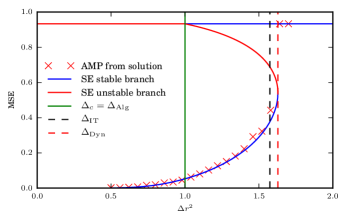
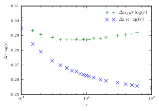
Figure 11: Left: We plot MSE deduced from state evolution (lines) and from Low-RAMP algorithm (marks) for $r=15$ groups and $N=20000$ as a function of $\Delta r^{2}$. The vertical full green line is $\Delta_{c}r^{2}=1$. The vertical dashed black line is $\Delta_{\rm IT}$ and the full lines correspond to the MSE obtained from the informative initialization and have discontinuities at $\Delta_{\rm Dyn}$. Note that the MSE from does not go to zero at finite positive $\Delta$ instead at small noise one has ${\rm MSE}\sim\exp\left(-{\rm const.}/\Delta\right)$. Right: We plot $\Delta r\log{r}$ for the information theoretic $\Delta_{\rm IT}$ and dynamical spinodal $\Delta_{\rm Dyn}$ phase transitions obtained from the state evolution using the protocol described in Appendix E. We rescale the $\Delta$ in this way to compare with the large rank expansion in (266) and (267).

V.2 Large sparsity (small $\rho$) expansions

In existing literature the sparse PCA was mostly studied for sparsity levels that are much smaller than a finite fraction of the system size (as considered in this paper). In order to compare with existing results we hence devote this section to the study of small density $\rho$ expansions of the results obtained from the state evolution for some of the models studied.

V.2.1 Spiked Bernoulli, Rademacher-Bernoulli, and Gauss-Bernoulli models

For both the Rademacher-Bernoulli, and Gauss-Bernoulli models we have the uniform fixed point stable above $\Delta_{c}=\rho^{2}$, and in the leading order in $1/\rho$ we have $\Delta_{\rm alg}\sim_{\rho\to 0}\Delta_{c}=\rho^{2}$.

The small $\rho$ limit behaviour of the information theoretic $\Delta_{\rm IT}$ threshold and the dynamical spinodal threshold $\Delta_{\rm Dyn}$ are given by

Bernoulli    and     Rademacher-Bernoulli

$$\Delta_{\rm Dyn}(\rho) \sim {}_{\rho\rightarrow 0}\frac{-\rho}{2\log(\rho)}\,,$$ (235)

$$\Delta_{\rm IT}(\rho) \sim {}_{\rho\rightarrow 0}\frac{-\rho}{4\log(\rho)}\,,$$

Gaussian-Bernoulli

$$\Delta_{\rm Dyn}(\rho) \sim {}_{\rho\rightarrow 0}\frac{-\rho}{\log(\rho)}\max\left\{\frac{\frac{2\exp\left(\frac{-1}{\beta}\right)}{\sqrt{\pi\beta}}+{\rm erfc}\left(\frac{1}{\sqrt{\beta}}\right)}{\beta},\beta\in\mathbb{R}^{+}\right\}\sim 0.595\frac{-\rho}{\log(\rho)}\,,$$ (237)

$$\Delta_{\rm IT}(\rho)\sim_{\rho\rightarrow 0}\frac{-\rho}{\log(\rho)}\max\left\{\frac{\frac{2\exp\left(\frac{-1}{\beta}\right)}{\sqrt{\pi\beta}}+{\rm erfc}\left(\frac{1}{\sqrt{\beta}}\right)}{\beta},\right.\\ \left.\int_{0}^{\beta}{\rm d}u\,\frac{2\exp\left(\frac{-1}{u}\right)}{\sqrt{\pi u}}+\left(\frac{1}{\sqrt{u}}\right)=\frac{1}{2}\beta\left[\frac{2\exp\left(\frac{-1}{\beta}\right)}{\sqrt{\pi\beta}}+{\rm erfc}\left(\frac{1}{\sqrt{\beta}}\right)\right];\beta\in\mathbb{R}^{+}\right\}\sim 0.528\frac{-\rho}{\log(\rho)}\,.$$ (238)

The information theoretic transitions for all these 3 models scale like $O\left(\frac{-\rho}{\log(\rho)}\right)$ while the algorithmic transition scales like $O(\rho^{2})$. This means that for small $\rho$ there is a large gap between what is information theoretically and algorithmically achievable. Note at this point that the bounds derived in banks2016information for sparse PCA have the same leading order behaviour when $\rho$ is small as (235) and (V.2.1).

To derive the above small $\rho$ expressions we combine (202) and (204) and the following small $\rho$ limit of the state-evolution functions $f^{\rm SE}(x)$

$$\forall\beta\in\mathbb{R}^{+},\lim_{\rho\rightarrow 0}\frac{f^{\rm SE}(-\beta\log(\rho))}{\rho}=1(\beta>2),\,\textbf{Bernoulli}$$ (239)

$$\forall\beta\in\mathbb{R}^{+},\lim_{\rho\rightarrow 0}\frac{f^{\rm SE}(-\beta\log(\rho))}{\rho}=1(\beta>2),\,\textbf{Rademacher-Bernoulli}$$ (240)

$$\forall\beta\in\mathbb{R}^{+},\lim_{\rho\rightarrow 0}\frac{f^{\rm SE}(-\beta\log(\rho))}{\rho}=\frac{2\exp\left(\frac{-1}{\beta}\right)}{\sqrt{\beta\pi}}+{\rm erfc}\left(\frac{1}{\sqrt{\beta}}\right),\,\textbf{Gaussian-Bernoulli}$$ (241)

Here the functions $f^{\rm SE}$ are the state-evolution update functions stated in (212), (214) and (216) for the different models (when the model is clear from context we will omit the lower index specifying the model). The above is proven by deriving the state evolution equations for each of these models. The computation is done in appendix D.

V.2.2 Two balanced groups, limit of small planted subgraph

In this section we analyze the small $\rho$ limit for the two balanced groups of section V.1.3. From the definition of the function $f_{\rho}$ (221), and a computation done in appendix D we get

$$\lim_{\rho\rightarrow 0}f_{\rho}(-\beta\rho(1-\rho)\log(\rho(1-\rho)))={1}(\beta>2)\,.$$ (242)

By combining this with (202) and (204) one gets

$$\Delta_{\rm Dyn}(\rho) \sim {}_{\rho\rightarrow 0}\frac{1}{-2\rho(1-\rho)\log(\rho(1-\rho))}\,,$$ (243)

$$\Delta_{\rm IT}(\rho) \sim {}_{\rho\rightarrow 0}\frac{1}{-4\rho(1-\rho)\log(\rho(1-\rho))}\,.$$ (244)

The derivations of these limits is done in the appendix D.

Note that the limit of small $\rho$ in the two balanced groups model is closely related to the problem of planted clique. However, in the planted clique problem the size of the clique to recover is much smaller that the size of the graph, typically $O(\sqrt{N})$ for efficient recovery and $O(\log{N})$ for information theoretically possible recovery. Whereas our equation were derives when $\rho=O(1)$, we can try to see what would the above scaling imply for $k=\rho N=o(N)$. In the planted clique problem the first (smaller) group is fully connected, this means that the entry $C_{11}$ of the connectivity matrix $C$ (37) is equal to one. Therefore for $\rho\ll 1$ one has

$$\mu=(1-p_{\rm out})\rho\sqrt{N}\,.$$ (245)

Note that in the canonical definition of the planted clique problem the average degree of the nodes belonging to the clique are slightly larger than the average degree of the rest of the graph. The present case of balanced groups corresponds to a version of the planted clique problem where next to planting a clique a corresponding number of edges is added to the rest of the graph to ensure that the average degree of every node is the same.

Recalling the definition of $\Delta$ (218) for the community detection output channel, and using $\Delta_{c}=1$ for the spectral threshold, and $\Delta_{\rm IT}=-1/(4\rho\log\rho)$ for the information theoretic threshold at small $\rho$ we get

$$k_{c}=\sqrt{N}\sqrt{\frac{p_{\rm out}}{1-p_{\rm out}}}\,,$$ (246)

$$k_{\rm IT}=\log(N)\frac{4p_{\rm out}}{1-p_{\rm out}}\,.$$ (247)

We indeed recover the scaling known from the planted clique problem, see e.g. deshpande2015finding . The $p_{\rm out}$-dependent constant are indeed the tight constants (for efficient and information theoretically optimal recovery) for the balanced version of the planted clique where the expected degree of every node is the same independently of the fact in the node is in the clique or not.

V.2.3 Sparse PCA at small density $\rho$

We investigate here the small $\rho$ limit of the bipartite $UV^{\top}$ spiked Gaussian-Bernoulli, and Rademacher-Bernoulli model. We remind that $U\in{\mathbb{R}}^{N}$, $V\in{\mathbb{R}}^{M}$, while $\alpha=M/N$. In the model we consider that elements of $U$ are Gaussian of zero mean and unit variance, while $P_{V}$ is given by (33) for the Rademacher-Bernoulli model, and by (36) for the Gauss-Bernoulli model. The state evolution equations then read

$$m_{u}^{t} = \frac{\alpha m_{v}^{t}}{\Delta+\alpha m_{v}^{t}}\,,$$ (248)

$$m_{v}^{t+1} = f_{\rm Gauss-Bernoulli}^{\rm SE}\left(\frac{m_{u}^{t}}{\Delta}\right)\,,$$ (249)

$$m_{v}^{t+1} = f_{\rm Rademacher-Bernoulli}^{\rm SE}\left(\frac{m_{u}^{t}}{\Delta}\right)\,,$$ (250)

where $f^{\rm SE}_{\rm Gauss-Bernoulli}$ and $f^{\rm SE}_{\rm Rademacher-Bernoulli}$ are defined in (214) and (216) respectively. By combining these equations one gets

$$m_{v}^{t+1} = f_{\rm Gauss-Bernoulli}^{\rm SE}\left(\frac{\alpha m_{v}^{t}}{\Delta^{2}+\alpha\Delta m_{v}^{t}}\right)\,,$$ (251)

$$m_{v}^{t+1} = f_{\rm Rademacher-Bernoulli}^{\rm SE}\left(\frac{\alpha m_{v}^{t}}{\Delta^{2}+\alpha\Delta m_{v}^{t}}\right)\,.$$ (252)

Because in both these cases $P_{U}$ and $P_{V}$ have zero mean the state evolution equations will have the uniform fixed point at $(m_{u},m_{v})=(0,0)$. This fixed point becomes unstable when

$$\frac{\rho^{2}\alpha}{\Delta^{2}}>1,\text{or},\Delta<\Delta_{c}=\rho\sqrt{\alpha}\,.$$ (253)

Also in this case the stability transition $\Delta_{c}$ corresponds to the spectral transition where one sees informative eigenvalues get out of the bulk of the matrix $S$, as is known in the theory of low-rank perturbations of random matrices baik2005phase (these methods are known not to take advantage of the sparsity). For $\rho$ small enough there will be again a first order phase transitions with $\Delta_{\rm Alg}$, $\Delta_{\rm IT}$, $\Delta_{\rm Dyn}$ defined as in section IV.3.1. The asymptotic behaviour of these thresholds is

Rademacher-Bernoulli

$$\Delta_{\rm Dyn}(\rho) \sim {}_{\rho\rightarrow 0}\sqrt{\frac{-\rho\alpha}{2\log(\rho)}}\,,$$ (254)

$$\Delta_{\rm IT}(\rho) \sim {}_{\rho\rightarrow 0}\sqrt{\frac{-\rho\alpha}{4\alpha\log(\rho)}}\,,$$

Gaussian-Bernoulli

$$\Delta_{\rm Dyn}(\rho) \sim {}_{\rho\rightarrow 0}\sqrt{\frac{-\rho\alpha}{\log(\rho)}\max\left\{\frac{{\rm erfc}\left(\frac{1}{\sqrt{\beta}}\right)}{\beta},\beta\in\mathbb{R}^{+}\right\}}\sim 0.771\sqrt{\frac{-\rho\alpha}{\log(\rho)}}\,,$$ (256)

$$\quad\quad\quad\quad\quad\quad\quad\quad\Delta_{\rm IT}(\rho)\sim_{\rho\rightarrow 0}\sqrt{\frac{-\rho\alpha}{\log(\rho)}}\\ \sqrt{\max\left\{\frac{\frac{2\exp\left(\frac{-1}{\beta}\right)}{\sqrt{\pi\beta}}+{\rm erfc}\left(\frac{1}{\sqrt{\beta}}\right)}{\beta},\int_{0}^{\beta}{\rm d}u\,\frac{2\exp\left(\frac{-1}{u}\right)}{\sqrt{\pi u}}+\left(\frac{1}{\sqrt{u}}\right)=\frac{1}{2}\beta\left[\frac{2\exp\left(\frac{-1}{\beta}\right)}{\sqrt{\pi\beta}}+{\rm erfc}\left(\frac{1}{\sqrt{\beta}}\right)\right];\beta\in\mathbb{R}^{+}\right\}}\\ \sim 0.726\sqrt{\frac{-\rho\alpha}{\log(\rho)}}\,.$$ (257)

Reminding that the value of $\Delta_{\rm Alg}$ scales in the same way as $\Delta_{c}$ (253), we see that a large hard phase opens as $\rho\to 0$.

To put the above results in relation to existing literature on sparse PCA amini2008high ; deshpande2014sparse . The main difference is that the regime considered in existing literature is that the number of non-zero element in the matrix $V$, $\rho N=o(1)$. The information theoretic threshold found in eq. (V.2.3) correspond (up to a constant) to information theoretic bounds found in amini2008high . However, the algorithmic performance that is found in the case of very small sparsity, by e.g. the covariance thresholding of deshpande2014sparse , is not reproduced in our analysis of linear sparsity $\rho=O(1)$. This suggest that in case when the sparsity is small but linear in $N$, efficient algorithms that take advantage of the sparsity might not exist. This regime should be investigated further.

To derive the small $\rho$ limit we follow a similar strategy as we did in the symmetric $XX^{\top}$ case. The main idea is to find the value of $\Delta$ for which $m_{v}=f^{\rm SE}_{P_{X}}(x)$ is a fixed point of the SE equations (252) or (251).

$$\Delta(x)=\frac{\alpha f^{\rm SE}(x)+\sqrt{\alpha^{2}{f^{\rm SE}}^{2}(x)+4\alpha\frac{f^{\rm SE}(x)}{x}}}{2}\,,$$ (258)

This means that

$$(m_{u},m_{v})=(x\Delta(x),f^{\rm SE}(x))$$ (259)

is a fixed point of the state evolution equations for $\Delta=\Delta(x)$. The free-energy is computed as

$$\phi(m_{u}=x\Delta(x),m_{v}=f(x),\Delta=\Delta(x))-\phi(m_{u}=0,m_{v}=0,\Delta=\Delta(x))=$$

$$=\alpha\int_{0}^{x}{\rm du}f^{\rm SE}(u)+\int_{0}^{\alpha f^{\rm SE}(x)/\Delta(x)}{\rm d}u\frac{u}{1+u}-xf^{\rm SE}(x)\,.$$ (260)

Combining this with (241) and (240) one gets the above asymptotic behaviour.

V.3 Large rank expansions

Another limit that can be worked out analytically is the large rank $r$ limit. This section summarizes the results.

V.3.1 Large-rank limit for jointly-sparse PCA

We analyze the large $r$ limit of jointly-sparse PCA for which the state evolution equation is given by (224). We notice that $u^{2}$ will have mean $r$ and standard deviation $\sqrt{2r}$. This essentially means that to get the large $r$ limit of the density evolution equations one need to replace $u^{2}$ by $r$ everywhere it appears. Expanding in large $r$ then gives

$$m^{t+1}=\frac{\rho m^{t}}{m^{t}+\Delta}\left(1+\frac{m^{t}}{\Delta}(1-\hat{\rho})\right)\hat{\rho}\,,$$ (261)

where

$$\hat{\rho}=\lim\limits_{r\rightarrow+\infty}\frac{\rho}{(1-\rho)\exp\left(\frac{r}{2}\left[\frac{m^{t}}{\Delta}+\log(1+\frac{m^{t}}{\Delta}\right)\right]+\rho}=\left\{\begin{matrix}1\,\,{\rm if}\,\,r{m^{t}}^{2}\rightarrow 0\\ \rho\,\,{\rm if}\,\,r{m^{t}}^{2}\rightarrow+\infty\end{matrix}\right.\,.$$ (262)

This means that for any $m^{t}\gg\frac{1}{\sqrt{r}}$ the update equations will be approximately

$$m^{t+1}=\frac{m^{t}\rho}{m^{t}+\Delta}+o(1)\,.$$ (263)

This update equation can be easily analyzed, it only has one stable fixed point located at

$$\max(\rho-\Delta,0)\,.$$ (264)

Analogous expansion of the replicated free energy leads to the result that in the large rank limit we have $\Delta_{\rm Dyn}=\Delta_{\rm IT}=\rho$ whereas $\Delta_{\rm Alg}=\Delta_{c}=\rho^{2}$. This is plotted in the large rank phase diagram (12).

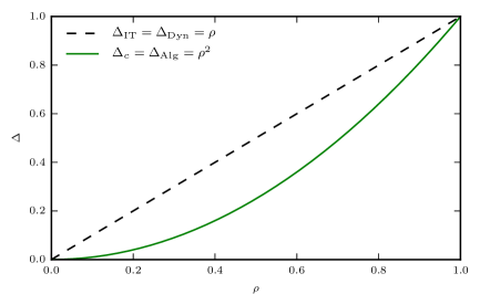
Figure 12: Phase diagram of the jointly-sparse PCA model at large rank $r$. In the large $r$ limit the algorithmic spinodal merges with $\Delta_{c}$, the dynamical spinodal and the information theoretic one converge toward the line $\Delta=\rho$.

V.3.2 Community detection

The large rank limit is analyzed for the problem of symmetric community detection in appendix E. The asymptotic behavior of $\Delta_{\rm IT}(r)$ and $\Delta_{\rm Dyn}(r)$ as $r\rightarrow+\infty$ are

$$\Delta_{c} = \frac{1}{r^{2}}\,,$$ (265)

$$\Delta_{\rm Dyn} = \frac{1}{2r\ln(r)}[1+o_{r}(1)]\,,$$ (266)

$$\Delta_{\rm IT} = \frac{1}{4r\ln(r)}[1+o_{r}(1)]\,.$$ (267)

We see that a large gap opens between $\Delta_{c}$ and $\Delta_{\rm IT}$ as $r$ grows. The behavior $\Delta_{\rm IT}$ and $\Delta_{\rm Dyn}$ for moderately large $r$ is illustrated in figure 11 and we see that the above limit is reached very slowly. Using eq. (229) this translates into the large $r$ limit phase transition in terms of parameters of the stochastic block model as discussed in lesieur2015mmse , and proven in banks2016information .

VI Discussion and perspective

The main results of this paper are summarised in section I.5. This concluding section is devoted to open directions and questions.

In this paper we considered models that lead to fully connected graphical models. It should be noted that the results and phase diagrams derived here in this setting are expected to hold as long as the average degree of the underlying factor graph is large enough (goes to infinity, after the $N\to\infty$ limit has been taken). Such expectation was proved rigorously in some special cases, see e.g. deshpande2016asymptotic ; caltagirone2016recovering .

A large part of results reported in this paper concerns the Bayes-optimal setting for which the mutual information and MMSE was recently established rigorously barbier2016mutual ; LelargeMiolane16 ; miolane2017fundamental .

A formidable open question concerns the nature of the hard phase, that is the region of parameters for which Low-RAMP does not reach the MMSE. Such regions have been identified in a considerable number of inference problems and it remains a great challenge to study whether efficient algorithms that perform better than Low-RAMP exist or to provide further evidence towards their non-existence. One notable direction is that whereas the MMSE in Bayes-optimal setting is correctly described by the replica symmetric solution, the nature of the metastable branch describing the behaviour of Low-RAMP in the hard phase may involve effect of replica symmetry breaking, this should be investigated in future work.

The results presented in this paper focused on the Bayes-optimal inference, the theory and methodology presented is not limited to this case and phase diagrams involving mismatch between the teacher and student models or parameters could provide further insight into issues such as model and parameter selection and learning, overfitting, or performance of minimisation-based algorithms. Effects of replica symmetry breaking are expected to play a role in this case. This is another interesting direction for future work.

In the present paper we focused on pair-wise interaction corresponding to matrix factorizations. In physics as well as in statistics a generalization to $p$-spin interaction have been studied. In statistics this type of problems is termed tensor PCA richard2014statistical . Detailed study of tensor PCA is also an interesting extension.

In the present paper we treated real-valued vectors spins. The generalization to spin-values that live on more involved spaces such as compact groups was recently considered in perry2016message and many interesting questions in this direction remain open.

Finally in the present work we concentrated on the theoretical development and phase diagrams for randomly generated data. The Low-RAMP algorithm (that is distributed in Matlab and Julia at http://krzakala.github.io/LowRAMP/ ) can be successfully applied to real-world data. In that case the set of theoretical guarantees on its performance is limited, but this is the case common to many other practically used approaches. Investigating performance of the Low-RAMP algorithm on data coming from applications of interest is another formidably rich and important direction for future work.

VII Acknowledgement

FK acknowledges funding from the EU (FP/2007-2013/ERC grant agreement 307087-SPARCS). LZ acknowledges funding for the project SaMURai from LabEx PALM (Ref : ANR-10-LABX-0039-PALM). We would like to thank Marc Mézard, Cristopher Moore, Pierfrancesco Urbani, and Christian Schmidt for discussions related to this work, and also Stefano Sarao, Fabrizio Antenucci, and Alexis Bozio for proofreading of the manuscript.

Appendix A Mean Field equations

In order to compare the Low-RAMP algorithm with the commonly used variational mean field inference we write here the variational mean field equations in the same notation we used for Low-RAMP. We also write the mean field free energy.

For the symmetric vector-spin glass the naive mean field equations read

$$B_{X,i}^{t} = \sum\limits_{k=1}^{N}\frac{1}{\sqrt{N}}S_{ki}{\hat{x}}_{k}^{t}\,,$$ (268)

$$A_{X,i}^{t} = \frac{1}{N}\sum\limits_{k=1}^{N}(S_{ki}^{2}-R_{ki})\left({{\hat{x}}_{k}^{t}{{\hat{x}}_{k}^{t,\top}+\sigma_{x,k}^{t}}}\right)\,,$$ (269)

$${\hat{x}}_{i}^{t+1} = f_{\rm in}^{x}(A_{X,i}^{t},B_{X,i}^{t})\,,$$ (270)

$$\sigma_{x,i}^{t+1} = \frac{\partial f_{\rm in}^{x}}{\partial B}(A_{X,i}^{t},B_{X,i}^{t})\,.$$ (271)

The mean field free energy for the symmetric $XX^{\top}$ case reads

$$F_{XX^{\top}}^{\rm MF}(\{A_{X,i}\},\{B_{X,i}\})=\sum\limits_{1\leq i\leq N}\log({\cal Z}_{x}(A_{X,i},B_{X,i}))-B_{X,i}^{\top}{\hat{x}}_{i}+\frac{1}{2}{\rm Tr}\left[A_{X,i}({\hat{x}}_{i}{\hat{x}}_{i}^{\top}+\sigma_{x,i})\right]\\ +\frac{1}{2}\sum\limits_{1\leq i,j\leq N}\left[\frac{1}{\sqrt{N}}S_{ij}{\hat{x}}_{i}^{\top}{\hat{x}}_{j}+\frac{(R_{ij}-S_{ij}^{2})}{2N}{\rm Tr}\left[({\hat{x}}_{i}{\hat{x}}_{i}^{\top}+\sigma_{x,i})({\hat{x}}_{j}{\hat{x}}_{j}^{\top}+\sigma_{x,j})\right]\right]\,.$$ (272)

For the bipartite $IUV^{\top}$ case the mean field equations read

$$B^{t}_{U,i} = \frac{1}{\sqrt{N}}\sum\limits_{l=1}^{M}S_{il}\hat{v}^{t}_{l}\,,$$ (273)

$$A_{U}^{t} = \frac{1}{N}\sum\limits_{l=1}^{M}\left(S_{il}^{2}-R_{il}\right)\left(\hat{v}_{l}^{t}{\hat{v}_{l}^{t,\top}}+\sigma_{u,l}^{t}\right)\,,$$ (274)

$$\hat{u}^{t}_{i} = f^{u}_{\rm in}(A^{t}_{U},B^{t}_{U,i})\,,$$ (275)

$$\sigma^{t}_{u,i} = \left(\frac{\partial f^{u}_{\rm in}}{\partial B}\right)(A^{t}_{U},B^{t}_{U,i})\,,$$ (276)

$$B^{t}_{V,j} = \frac{1}{\sqrt{N}}\sum\limits_{k=1}^{N}S_{kj}\hat{u}_{k}^{t}\,,$$ (277)

$$A_{V,j}^{t} = \frac{1}{N}\sum\limits_{k=1}^{N}(S_{kj}^{2}-R_{kj})\left(\hat{u}_{k}^{t}{\hat{u}_{k}^{t,\top}}+\sigma_{u,k}^{t}\right)\,,$$ (278)

$$\hat{v}^{t+1}_{j} = f^{v}_{\rm in}(A^{t}_{V,j},B^{t}_{V,j})\,,$$ (279)

$$\sigma^{t+1}_{v,j} = \left(\frac{\partial f^{v}_{\rm in}}{\partial B}\right)(A^{t}_{V,j},B^{t}_{V,j})\,.$$ (280)

The mean field free energy for the bipartite case reads

$$F_{UV^{\top}}^{\rm MF}(\{A_{U,i}\},\{B_{U,i}\},\{A_{V,j}\},\{B_{V,j}\})=\sum\limits_{1\leq i\leq N}\log({\cal Z}_{u}(A_{U,i},B_{U,i}))-{B_{U,i}}^{\top}{\hat{u}}_{i}+\frac{1}{2}{\rm Tr}\left[A_{U,i}({\hat{u}}_{i}{\hat{u}}_{i}^{\top}+\sigma_{u,i})\right]\\ +\sum\limits_{1\leq j\leq M}\log({\cal Z}_{v}(A_{V,j},B_{V,j}))-{B_{V,j}}^{\top}{\hat{v}}_{j}+\frac{1}{2}{\rm Tr}\left[A_{V,j}({\hat{v}}_{j}{\hat{v}}_{j}^{\top}+\sigma_{v,j})\right]\\ +\sum\limits_{1\leq i\leq N,1\leq j\leq M}\left[\frac{1}{\sqrt{N}}S_{ij}\hat{u}_{i}^{\top}\hat{v}_{j}+\frac{1}{2N}(R_{ij}-S_{ij}^{2}){\rm Tr}\left[(\hat{u}_{i}\hat{u}_{i}^{\top}+\sigma_{u,i})(\hat{v}_{j}\hat{v}_{j}^{\top}+\sigma_{v,j})\right]\right]\,.$$ (281)

The difference between the mean field equations and the Low-RAMP equations from section II.2 and II.4 can be seen for both variables $A$ and $B$.

Appendix B Bethe free energy derived by the Plefka expansion

We present here a way to compute the Bethe free energy for relatively generic class of Hamiltonians. The main hypothesis for this computation to be exact in the large $N$ limit is that the Fisher score matrix $S_{ij}$ can be well approximated as having elements with weak correlation of order $\frac{1}{N}$ one from another. If this is not true then the following equations do not apply.

As it turns out the mean-field free energy from Appendix A is just the first order term in the high temperature expansion of the free-energy. as was derived in [67, 72] first by Plefka and then by Georges and Yedidia. The Bethe free energy is then the 2nd order expansion. Suppose one is given a general system with with $N$ classical variables $x_{i}$ that weakly interact. The Hamiltonian $H$ defined the free energy

$$\Phi=\log\left({\rm Tr}\left[\exp(\beta H(x_{1},\cdots,x_{N}))\right]\right)\,.$$ (282)

We define a new Hamiltonian that fixes the marginal by

$$\beta H_{\rm Field}(\{\lambda_{i}\})=\beta H+\sum\limits_{1\leq i\leq N}\lambda_{i}(x_{i},\beta)\,,$$ (283)

$$\Phi_{\rm Field}(\beta,\{\lambda_{i}\})=\log\left({\rm Tr}\left[\exp(\beta H_{\rm Field}(\{\lambda_{i}\}))\right]\right)\,.$$ (284)

By taking the Legendre transform one gets

$$\Phi_{\rm Legendre}(\beta,\{\mu_{i}(x_{i})\}) = \min\left\{\Phi_{\rm Field}(\beta,\{\lambda_{i}\})-\sum\limits_{1\leq i\leq n}\int{\rm d}x\mu_{i}(x)\lambda_{i}(x)\right\}\,,$$ (285)

$$\{\Lambda_{i}(x_{i})\} = {\rm argmin}\left\{\Phi_{\rm Field}(\beta,\{\lambda_{i}\})-\sum\limits_{1\leq i\leq n}\int{\rm d}x\mu_{i}(x)\lambda_{i}(x)\right\}\,,$$ (286)

here the minimization is done over the fields $\lambda_{i}(x_{i})$. The $\mu_{i}(x_{i})$ are marginal density probabilities that one aims to impose on the system. The $\Lambda_{i}(x_{i})$ are the fields one uses to fix the marginals equal to $\mu_{i}(x_{i})$. The $\Lambda_{i}(x_{i})$ depend on the problem $H$, $\beta$ and the $\mu_{i}(x_{i})$. Because the $\Lambda_{i}(x_{i})$ are defined up to a constant

$$\int{\rm d}x\mu_{i}(x)\Lambda_{i}(x)=0$$ (287)

is imposed. According to the definition of the Legendre transformation on has

$$\Phi=\max\left\{\Phi_{\rm Legendre}(\beta,\{\mu_{i}(x_{i})\})\right\}\,.$$ (288)

To compute $\Phi_{\rm Legendre}(\beta,\{\mu_{i}(x_{i})$ we resort to a high temperature expansion. This procedure is called the Plefka expansion [67], it relies on the following high temperature expansion (we stop at order 2)

$$\Phi_{\rm Bethe}=\Phi_{\rm Frustrated}(\beta=0)+\beta\left(\frac{\partial\Phi_{\rm Legendre}}{\partial\beta}\right)(\beta=0)+\frac{\beta^{2}}{2}\left(\frac{\partial^{2}\Phi_{\rm Legendre}}{\partial\beta^{2}}\right)(\beta=0)\,.$$ (289)

The expansion was explained in detail in [72], here we remind the main steps. Let us introduce the following operator

$$U=H-\langle H\rangle-\sum\limits_{1\leq i\leq N}\frac{\partial\Lambda_{i}(x_{i})}{\partial\beta}\,,$$ (290)

where the average is taken with respect to probability distribution induced by (283). One can show that for all observables $O$ one has

$$\forall\beta,\frac{\partial\langle O\rangle}{\partial\beta}=\left\langle\frac{\partial O}{\partial\beta}\right\rangle-\langle OU\rangle\,.$$ (291)

According to the definition of $F_{\rm Frustrated}$ one can prove that.

$$\forall\beta,\frac{\partial\Phi_{\rm Legendre}}{\partial\beta}=\langle H\rangle\,.$$ (292)

Using (292) and (291) we get

$$\forall\beta,\frac{\partial^{2}\Phi_{\rm Legendre}}{\partial\beta^{2}}=\frac{\langle H\rangle}{\partial\beta}=-\langle HU\rangle\,.$$ (293)

Therefore

$$\Phi_{\rm Bethe}=\Phi_{\rm Legendre}(\beta=0)+\beta\langle H\rangle(\beta=0)-\frac{\beta^{2}}{2}\langle HU\rangle(\beta=0)\,.$$ (294)

We still need to compute $\frac{\partial\Lambda_{i}(x_{i})}{\partial\beta}$ at $\beta=0$. This can be done by computing the derivative of the marginals with respect to $\beta$ and noticing that they have to be zero.

$$\left(\frac{\partial\langle\delta(x_{i}-\hat{x}_{i})\rangle}{\partial\beta}\right)=\left(\frac{\partial\mu_{i}(\hat{x}_{i})}{\partial\beta}\right)=0=\langle U\delta(x_{i}-\hat{x}_{i})\rangle=\left\langle\left(H-<H>-\sum\limits_{1\leq i\leq N}\frac{\partial\Lambda_{i}(x_{i})}{\partial\beta}+\int{\rm d}\hat{x}_{i}\mu_{i}(\hat{x}_{i})\frac{\partial\Lambda_{i}(\hat{x}_{i})}{\partial\beta}\right)\delta(x_{i}-\hat{x}_{i})\right\rangle\,.$$ (295)

From this one deduces

$$\left\langle\frac{\partial\Lambda_{i}(x_{i})}{\partial\beta}\delta(x_{i}-\hat{x}_{i})+C(i,\beta)\delta(x_{i}-\hat{x}_{i})s\right\rangle=\langle H\delta(x_{i}-\hat{x}_{i})-\langle H\rangle\delta(x_{i}-\hat{x}_{i})\rangle\,,$$ (296)

where $C({i,\beta})$ is

$$C(i,\beta)=\int{\rm d}\hat{x}_{i}\mu_{i}(\hat{x}_{i})\frac{\partial\Lambda_{i}(\hat{x}_{i})}{\partial\beta}\,.$$ (297)

By definition

$$\langle\delta(x_{i}-\hat{x}_{i})\rangle = \mu_{i}(\hat{x}_{i})\,,$$ (298)

$$\langle H\delta(x_{i}-\hat{x}_{i})\rangle = \mu_{i}(x_{i})\langle H\rangle_{x_{i}=\hat{x}_{i}}\,,$$ (299)

where $\langle H\rangle_{x_{i}=\hat{x}_{i}}$ is the average energy conditioned on the fact that $x_{i}=\hat{x}_{i}$. Using (296) we get

$$\mu_{i}(\hat{x_{i}})\left(\frac{\partial\Lambda_{i}(\hat{x}_{i})}{\partial\beta}\right)=\mu_{i}(\hat{x_{i}})\langle H\rangle_{x_{i}=\hat{x}_{i}}-\mu_{i}(\hat{x_{i}})\langle H\rangle+\mu_{i}(\hat{x_{i}})C(i,\beta)\,,$$ (300)

$$\left(\frac{\partial\Lambda_{i}(\hat{x}_{i})}{\partial\beta}\right)=\langle H\rangle_{x_{i}=\hat{x}_{i}}-\langle H\rangle+C(i,\beta)\,.$$ (301)

We can see from (283) that $\Lambda_{i}(\hat{x}_{i},\beta)$ is defined up to a constant we fix that constant by having

$$\int{\rm d}\hat{x}_{i}\mu_{i}(\hat{x}_{i})\Lambda_{i}(\hat{x}_{i})=0\,.$$ (302)

Therefore we get

$$\forall\beta,\left(\frac{\partial\Lambda_{i}(\hat{x}_{i})}{\partial\beta}\right)=\langle H\rangle_{x_{i}=\hat{x}_{i}}-\langle H\rangle\ =\frac{1}{\mu_{i}(\hat{x}_{i})}\langle H\delta(x_{i}-\hat{x}_{i})\rangle-\langle H\rangle\,,$$ (303)

where once again $\langle H\rangle_{x_{i}=\hat{x}_{i}}$ is the average of the energy where we have conditioned on the event $x_{i}=\hat{x_{i}}$. Since we do all expansion around $\beta=0$ one is able to compute all the means present in this formula since at $\beta=0$ the density probability of the system at $\beta=0$ is just

$$P_{\rm Factorised}=\prod\limits_{i=1\cdots N}\mu_{i}(x_{i})\,.$$ (304)

By using (289) and (303) around $\beta=0$ one gets

$$\Phi_{\rm Bethe}=\sum\limits_{1\leq i\leq N}S_{\mu_{i}}+\beta\langle H\rangle+\frac{\beta^{2}}{2}\left[\langle H^{2}\rangle-\langle H\rangle^{2}-\sum\limits_{1\leq i\leq N}\int{\rm d}x_{i}\mu_{i}(\hat{x}_{i})(\langle H\rangle_{x_{i}=\hat{x}_{i}}-\langle H\rangle)^{2}\right]\,,$$ (305)

where here $S_{\mu_{i}}$ is here the entropy of the density probability $\mu_{i}(x_{i})$. In this setting all terms of order $3$ and beyond will give a zero contribution in the large $N$ limit. This is due to the fact that the matrix $Y$ has components largely uncorrelated since they were taken independently from one another (the signal induces correlation that are too small to be significant). One reason why this approach might fail is that even though order higher than 3 might disappears in the large $N$ limit their sum might be non convergent. This is the sign of a replica symmetry breaking in the system.

From this expression we deduce the Bethe free energy for the $XX^{\top}$ case as a function of the variables $A_{X,i}$ and $B_{X,i}$. The marginals that will be enforced are

$$P_{X,{\rm Marginal}}(x_{i})=\frac{1}{{\cal Z}_{x}(A_{X,i},B_{X,i})}P_{X}(x_{i})\exp\left(B_{X,i}^{\top}x_{i}-\frac{x_{i}^{\top}A_{X,i}x_{i}}{2}\right)\,,$$ (306)

$$P_{U,{\rm Marginal}}(u_{i})=\frac{1}{{\cal Z}_{u}(A_{U,i},B_{U,i})}P_{U}(u_{i})\exp\left(B_{U,i}^{\top}u_{i}-\frac{u_{i}^{\top}A_{U,i}u_{i}}{2}\right)\,,$$ (307)

$$P_{V,{\rm Marginal}}(v_{j})=\frac{1}{{\cal Z}_{v}(A_{V,j},B_{V,j})}P_{X}(v_{j})\exp\left(B_{V,i}^{\top}v_{j}-\frac{v_{j}^{\top}A_{V,j}v_{j}}{2}\right)\,.$$ (308)

The Hamiltonians are

$$H_{XX^{\top}}=\sum\limits_{i=1\cdots N}\log(P_{X}(x_{i}))+\sum\limits_{1\leq i<j\leq N}\left[g\left(Y_{ij},\frac{x_{i}^{\top}x_{j}}{\sqrt{N}}\right)-g(Y_{ij},0)\right]\,,$$ (309)

and

$$H_{UV^{\top}}=\sum\limits_{i=1\cdots N}\log(P_{U}(u_{i}))+\sum\limits_{j=1\cdots M}\log(P_{V}(v_{j}))+\sum\limits_{1\leq i\leq N,1\leq j\leq M}\left[g\left(Y_{ij},\frac{u_{i}^{\top}v_{j}}{\sqrt{N}}\right)-g(Y_{ij},0)\right]\,.$$ (310)

Using (306,307,308) and (309,310) in (305) one gets for the symmetric $XX^{\top}$ case

$$\Phi_{XX^{\top}}(\{A_{X,i}\},\{B_{X,i}\})=\sum\limits_{1\leq i\leq N}\left[\log({\cal Z}_{x}(A_{X,i},B_{X,i}))-B_{X,i}^{\top}{\hat{x}}_{i}+\frac{1}{2}{\rm Tr}\left[A_{X,i}({\hat{x}}_{i}{\hat{x}}_{i}^{\top}+\sigma_{x,i})\right]\right]\\ +\frac{1}{2}\sum\limits_{1\leq i,j\leq N}\left[\frac{1}{\sqrt{N}}S_{ij}{\hat{x}}_{i}^{\top}{\hat{x}}_{j}+\frac{R_{ij}}{2N}{\rm Tr}\left[({\hat{x}}_{i}{\hat{x}}_{i}^{\top}+\sigma_{x,i})({\hat{x}}_{j}{\hat{x}}_{j}^{\top}+\sigma_{x,j})\right]-\frac{S_{ij}^{2}}{2N}{\rm Tr}\left[{\hat{x}}_{i}{\hat{x}}_{i}^{\top}{\hat{x}}_{j}{\hat{x}}_{j}^{\top}\right]-\frac{1}{N}S_{ij}^{2}{\rm Tr}\left[\sigma_{x,i}\sigma_{x,j}\right]\right]\,.$$ (311)

For the $UV^{\top}$ case

$$\Phi_{{\rm Bethe},UV^{\top}}(\{A_{U,i}\},\{B_{U,i}\},\{A_{V,j}\},\{B_{V,j}\})=\sum\limits_{1\leq i\leq N}\left[\log({\cal Z}_{u}(A_{U,i},B_{U,i}))-{B_{U,i}}^{\top}{\hat{u}}_{i}+\frac{1}{2}{\rm Tr}\left[A_{U,i}({\hat{u}}_{i}{\hat{u}}_{i}^{\top}+\sigma_{u,i})\right]\right]\\ +\sum\limits_{1\leq j\leq M}\left[\log({\cal Z}_{v}(A_{V,j},B_{V,j}))-{B_{V,j}}^{\top}{\hat{v}}_{j}+\frac{1}{2}{\rm Tr}\left[A_{V,j}({\hat{v}}_{j}{\hat{v}}_{j}^{\top}+\sigma_{v,j})\right]\right]\\ +\sum\limits_{1\leq i\leq N,1\leq j\leq M}\left[\frac{1}{\sqrt{N}}S_{ij}\hat{u}_{i}^{\top}\hat{v}_{j}+\frac{1}{2N}R_{ij}{\rm Tr}\left[(\hat{u}_{i}\hat{u}_{i}^{\top}+\sigma_{u,i})(\hat{v}_{j}\hat{v}_{j}^{\top}+\sigma_{v,j})\right]-\frac{S_{ij}^{2}{\rm Tr}\left(\hat{u}_{i}\hat{u}_{i}^{\top}\hat{v}_{j}\hat{v}_{j}^{\top}\right)}{2N}-\frac{1}{N}S_{ij}^{2}{\rm Tr}\left[\sigma_{u,i}\sigma_{v,j}\right]\right]\,,$$ (312)

where the $\hat{x}_{i},\hat{u}_{i},\hat{v}_{j},\sigma_{x,i},\sigma_{u,i},\sigma_{v,j}$ are the mean of the marginals we want to enforce. These are all function of variables $B_{i}$, and $A_{i}$. One should try and minimize these function. This is what Low-RAMP does. Fixed points of the Low-RAMP algorithm are stationary points of the of the Bethe free energy.

Appendix C Replica computation $UV^{\top}$ case.

In this appendix we present the derivation replica free-energy in the case of the $UV^{\top}$ case. In the coming computation the indices $i$ and $k$ will go from $1$ to $N$. And $j$ and $l$ will go from $1$ to $M$.

$${\cal Z}(\{Y_{ij}\})=\int\prod_{i}{\rm d}u_{i}P_{U}({u}_{i})\prod_{j}{\rm d}v_{j}P_{U}({v}_{j})\prod_{ij}\exp\left(g\left(Y_{ij},\frac{u_{i}^{\top}v_{j}}{\sqrt{N}}\right)-g\left(Y_{ij},0\right)\right)\,.$$ (313)

One would like to compute the average of $\langle\log({\cal Z}(\{Y_{ij}\}))\rangle$. This can be computed using the replica trick

$$\langle\log({\cal Z}(\{Y_{ij}\}))\rangle_{Y}=\lim\limits_{n\rightarrow 0}\frac{\langle{\cal Z}^{n}\rangle-1}{n}=\lim\limits_{n\rightarrow 0}\frac{\log(\langle{\cal Z}^{n}\rangle)}{n}\,.$$ (314)

These can be hopefully be computed for any $n\in\mathbb{N}$. We will then compute this function as $n\rightarrow 0$. We start with evaluating

$${\cal Z}^{n}(\{Y_{ij}\})=\int\prod\limits_{a=1\cdots n}\prod\limits_{i=1\cdots N}{\rm d}u^{a}_{i}P^{a}_{U}(u^{a}_{i})\prod\limits_{j=1\cdots M}{\rm d}v^{a}_{j}P_{V}^{a}(v^{a}_{j})\exp\prod\limits_{i=1\cdots N,j=1\cdots M}\exp\left(g\left(Y_{ij},\frac{u_{i}v_{j}}{\sqrt{N}}\right)-g\left(Y_{ij},0\right)\right)\,.$$ (315)

Therefore one has

$$\mathbb{E}({\cal Z}^{n})=\int\prod\limits_{i=1\cdots N,j=1\cdots M}{\rm d}Y_{ij}P_{\rm out}\left(Y_{ij},w=0\right)\prod\limits_{a=0\cdots n}\left(\left[\prod\limits_{i=1\cdots N}{\rm d}u^{a}_{i}P_{U}^{a}(u^{a}_{i})\prod\limits_{j=1\cdots M}{\rm d}v^{a}_{j}P_{V}^{a}(v^{a}_{j})\right]\right.\\ \left.\left[\prod\limits_{i=1\cdots N,j=1\cdots M}\exp\left(\sum\limits_{a=0\cdots n}g^{a}\left(Y_{ij},\frac{u_{i}^{a}v_{j}^{a}}{\sqrt{N}}\right)-g^{a}\left(Y_{ij},0\right)\right)\right]\right)\,,$$ (316)

where

• if $a=0$ then $g^{a}=g^{0}=\log(P_{\rm out}(Y,w))$, $P^{a}_{U}(u)=P_{U_{0}}(u)$ and $P^{a}_{V}(v)=P_{V_{0}}(v)$

• if $a\neq 0$ then $g^{a}=g$, $P_{U}^{a}(u)=P_{U}(u)$ and $P_{V}^{a}(v)=P_{V}(v)$

We expand the function $g^{a}$ to order 2 and get

$$\mathbb{E}({\cal Z}^{n})=\int\prod\limits_{i=1\cdots N,j=1\cdots M}{\rm d}Y_{ij}P_{\rm out}\left(Y_{ij},w=0\right)\prod\limits_{a=0\cdots n}\left(\left[\prod\limits_{i=1\cdots N}{\rm d}u^{a}_{i}P_{U}^{a}(u^{a}_{i})\prod\limits_{j=1\cdots M}{\rm d}v^{a}_{j}P_{V}^{a}(v^{a}_{j})\right]\right.\\ \left.\left[\prod\limits_{i=1\cdots N,j=1\cdots M}\exp\left(\sum\limits_{a=0\cdots n}\left(\frac{\partial g^{a}}{\partial w}\right)_{Y_{ij},0}\frac{u_{i}^{a}v_{j}^{a}}{\sqrt{N}}+\left(\frac{\partial^{2}g^{a}}{\partial w^{2}}\right)_{Y_{ij},0}\frac{(u_{i}^{a}v_{j}^{a})^{2}}{2N}+O\left(\frac{1}{N^{1}.5}\right)\right)\right]\right)\,.$$ (317)

By expanding the exponential to order two one gets

$$\mathbb{E}({\cal Z}^{n})=\int\prod\limits_{i=1\cdots N,j=1\cdots M}{\rm d}Y_{ij}P_{\rm out}\left(Y_{ij},w=0\right)\prod\limits_{a=0\cdots n}\left[\prod\limits_{i=1\cdots N}{\rm d}u^{a}_{i}P_{U}^{a}(u^{a}_{i})\prod\limits_{j=1\cdots M}{\rm d}v^{a}_{j}P_{V}^{a}(v^{a}_{j})\right]\\ \prod\limits_{i=1\cdots N,j=1\cdots M}\left[1+\sum\limits_{a=0\cdots n}\left(\frac{\partial g^{a}}{\partial w}\right)_{Y_{ij},0}\frac{u_{i}^{a}v_{j}^{a}}{\sqrt{N}}+\right.\\ \left.\sum\limits_{a=1\cdots n}\left(\frac{\partial g}{\partial w}\right)_{Y_{ij},0}\left(\frac{\partial g^{0}}{\partial w}\right)_{Y_{ij},0}\frac{u_{i}^{a}v_{j}^{a}u_{i}^{0}v_{j}^{0}}{N}+\sum\limits_{1\leq a<b\leq n}\left(\frac{\partial g}{\partial w}\right)_{Y_{ij},0}\left(\frac{\partial g}{\partial w}\right)_{Y_{ij},0}\frac{u_{i}^{a}v_{j}^{a}u_{i}^{b}v_{j}^{b}}{N}+\right.\\ \left.\sum\limits_{a=0\cdots n}\left[\left(\frac{\partial^{2}g^{a}}{\partial w^{2}}\right)_{Y_{ij},0}+\left(\frac{\partial^{2}g^{a}}{\partial w^{2}}\right)_{Y_{ij},0}^{2}\right]\frac{(u_{i}^{a}v_{j}^{a})^{2}}{2N}+O\left(\frac{1}{N^{1.5}}\right)\right]\,.$$ (318)

By averaging with respect to the $Y_{ij}$ one gets

$$\mathbb{E}({\cal Z}^{n})=\int\prod\limits_{a=0\cdots n}\left[\prod\limits_{i=1\cdots N}{\rm d}u^{a}_{i}P_{U}^{a}(u^{a}_{i})\prod\limits_{j=1\cdots M}{\rm d}v^{a}_{j}P_{V}^{a}(v^{a}_{j})\right]\\ \prod\limits_{i=1\cdots N,j=1\cdots M}\left[1+\sum\limits_{a=1\cdots n}\frac{u_{i}^{a}v_{j}^{a}u_{i}^{0}v_{j}^{0}}{N\widehat{\Delta}}+\sum\limits_{1\leq a<b\leq n}\frac{u_{i}^{a}v_{j}^{a}u_{i}^{b}v_{j}^{b}}{N\widetilde{\Delta}}+\sum\limits_{a=1\cdots n}\overline{R}\frac{(u_{i}^{a}v_{j}^{a})^{2}}{2N}+O\left(\frac{1}{N^{1.5}}\right)\right]\,.\\ =\int\left[\prod\limits_{a=0\cdots n}\prod\limits_{i=1\cdots N}{\rm d}u^{a}_{i}P_{U}^{a}(u^{a}_{i})\prod\limits_{j=1\cdots M}{\rm d}v^{a}_{j}P_{V}^{a}(v^{a}_{j})\right]\\ \exp\left(\sum\limits_{i=1\cdots N,j=1\cdots M}\sum\limits_{a=1\cdots n}\frac{u_{i}^{a}v_{j}^{a}u_{i}^{0}v_{j}^{0}}{N\widehat{\Delta}}+\sum\limits_{1\leq a<b\leq n}\frac{u_{i}^{a}v_{j}^{a}u_{i}^{b}v_{j}^{b}}{N\widetilde{\Delta}}+\sum\limits_{a=1\cdots n}\overline{R}\frac{(u_{i}^{a}v_{j}^{a})^{2}}{2N}+O\left(\frac{1}{N^{1.5}}\right)\right)\,.$$ (319)

We now introduce the order parameters

$$q^{u}_{ab}=\frac{1}{N}\sum\limits_{i=1\cdots N}u_{i}^{a}u_{i}^{b}\,,$$ (320)

$$q^{v}_{ab}=\frac{1}{M}\sum\limits_{j=1\cdots M}v_{j}^{a}v_{j}^{b}\,.$$ (321)

This leads to

$$\mathbb{E}({\cal Z}^{n})=NM\int\prod_{0\leq a\leq b\leq n}{\rm d}q^{u}_{ab}{\rm d}q^{v}_{ab}\exp\left(\frac{N\alpha}{\widehat{\Delta}}\sum\limits_{a=1\cdots n}q^{u}_{a0}q^{v}_{a0}+\frac{N\alpha}{\widetilde{\Delta}}\sum\limits_{1\leq a<b\leq n}q^{u}_{ab}q^{v}_{ab}+\frac{N\alpha}{2}\sum\limits_{a=\cdots n}\overline{R}q^{u}_{aa}q^{v}_{aa}\right)\hat{\mathit{I}}_{u}(\{q^{u}_{ab}\})\hat{\mathit{I}}_{v}(\{q^{v}_{ab}\})\,,$$ (322)

where

$$\hat{\mathit{I}}_{u}(\{q^{u}_{ab}\})=\int\left(\prod\limits_{a=1\cdots n}\prod\limits_{i=1\cdots N}{\rm d}u^{a}_{i}P_{V}^{a}(u^{a}_{i})\right)\prod\limits_{0\leq a\leq b\leq n}\delta\left(\sum\limits_{i=1\cdots N}u_{i}^{a}u_{i}^{b}-Nq^{u}_{ab}\right)\,,$$ (323)

and

$$\hat{\mathit{I}}_{v}(\{q^{v}_{ab}\})=\int\left(\prod\limits_{a=1\cdots n}\prod\limits_{j=1\cdots M}{\rm d}v^{a}_{j}P_{V}^{a}(v^{a}_{j})\right)\prod\limits_{0\leq a\leq b\leq n}\delta\left(\sum\limits_{i=1\cdots N}v_{j}^{a}v_{j}^{b}-Mq^{v}_{ab}\right)\,.$$ (324)

Here $\hat{\mathit{I}}_{u}(\{q^{u}_{ab}\})$ and $\hat{\mathit{I}}_{v}(\{q^{v}_{ab}\})$ are the entropy costs one pays in order for the order parameters to take one specific value. We can treat this constraint by going to Fourier space and then rotating the path of integration

$$\mathit{I}_{u}(\{q^{u}_{ab}\},\{\hat{q}^{u}_{ab}\})=\int\prod\limits_{a=0\cdots n}P_{U}^{a}(u_{a}){\rm d}u^{a}\exp\left(\sum\limits_{0\leq a\leq b\leq n}\hat{q}^{u}_{ab}({u^{a}}u^{b}-q^{u}_{ab})\right)\,.$$ (325)

$$\mathit{I}_{v}(\{q^{v}_{ab}\},\{\hat{q}^{v}_{ab}\})=\int\prod\limits_{a=0\cdots n}P_{V}^{a}(v_{a}){\rm d}v^{a}\exp\left(\sum\limits_{0\leq a\leq b\leq n}\hat{q}^{v}_{ab}({v^{a}}v^{b}-q^{v}_{ab})\right)\,.$$ (326)

Therefore

$$\mathbb{E}({\cal Z}^{n})=NM\int\prod_{0\leq a\leq b\leq n}{\rm d}q^{u}_{ab}{\rm d}\hat{q}^{u}_{ab}{\rm d}q^{v}_{ab}{\rm d}\hat{q}^{v}_{ab}\exp\left(\frac{N\alpha}{\widehat{\Delta}}\sum\limits_{a=1\cdots n}q^{u}_{a0}q^{v}_{a0}+\frac{N\alpha}{\widetilde{\Delta}}\sum\limits_{1\leq a<b\leq n}q^{u}_{ab}q^{v}_{ab}+\frac{N\alpha}{2}\sum\limits_{a=\cdots n}\overline{R}q^{u}_{aa}q^{v}_{aa}\right)\\ +\mathit{I}_{u}(\{q^{u}_{ab}\},\{\hat{q}^{u}_{ab}\}))^{N}+\mathit{I}_{v}(\{q^{v}_{ab}\},\{\hat{q}^{v}_{ab}\}))^{M}$$ (327)

We need to extremize this function with respect to all variables. By taking the derivative equal to 0 with respect to variables $q^{u}_{ab}$ and $q^{v}_{ab}$ we get

$$\hat{q}_{a0}^{u} = \frac{\alpha\hat{q}_{a0}^{v}}{\widehat{\Delta}},\qquad\hat{q}_{a0}^{v}=\frac{\hat{q}_{a0}^{u}}{\widehat{\Delta}}\,,$$ (328)

$$\forall 1\leq a<b\leq n,\quad\quad\hat{q}_{ab}^{u} = \frac{\alpha\hat{q}_{ab}^{v}}{\widetilde{\Delta}},\qquad\hat{q}_{ab}^{v}=\frac{\hat{q}_{ab}^{u}}{\widetilde{\Delta}}\,,$$ (329)

$$\hat{q}_{aa}^{u} = \overline{R}\alpha\hat{q}_{ab}^{v},\qquad\hat{q}_{ab}^{v}=\overline{R}\hat{q}_{ab}^{u}\,.$$ (330)

We now assume the replica symmetric ansatz

$$\forall a,b>1,\quad q_{ab}^{u} = \delta^{a}_{b}(\Sigma_{u}+Q_{u})+(1-\delta^{a}_{b})Q_{u}\,,$$ (331)

$$\forall a>1,\quad q_{a0}^{u} = M_{u}\,,$$ (332)

$$\forall a,b>1,\quad q_{ab}^{v} = \delta^{a}_{b}(\Sigma_{v}+Q_{v})+(1-\delta^{a}_{b})Q_{v}\,,$$ (333)

$$\forall a>1,\quad q_{a0}^{v} = M_{v}\,.$$ (334)

We can then express the free energy. Let us compute $I_{u}$ and $I_{v}$ in that RS ansatz

$$\mathit{I}_{u}(\{q^{u}_{ab}\},\{\hat{q}^{u}_{ab}\})\exp\left(\sum\limits_{0\leq a\leq b\leq n}\hat{q}^{u}_{ab}q^{u}_{ab}\right)=\int\prod\limits_{a=0\cdots n}P_{U}^{a}(u_{a}){\rm d}u^{a}\exp\left(\sum\limits_{0\leq a\leq b\leq n}\hat{q}^{u}_{ab}{u^{a}}u^{b}\right)\,.$$ (335)

By using Hubbard-Stratonovich identity one gets

$$\mathit{I}_{u}(\{q^{u}_{ab}\},\{\hat{q}^{u}_{ab}\})\exp\left(\sum\limits_{0\leq a\leq b\leq n}\hat{q}^{u}_{ab}q^{u}_{ab}\right)=$$ (336)

$$=\int{\cal D}WP_{U_{0}}(u_{0}){\rm d}u^{0}\left[\int{\rm d}uP_{U}(u)\exp\left(\frac{\alpha M_{v}}{\widehat{\Delta}}uu_{0}+W\sqrt{\frac{\alpha Q_{v}}{\widetilde{\Delta}}}u-\left(\frac{\alpha Q_{v}}{\widetilde{\Delta}}-\alpha\overline{R}(Q_{v}+\Sigma_{v})\right)\frac{u^{2}}{2}\right)\right]^{n}\,.$$ (337)

We can now compute the limit as $n\rightarrow 0$.

$$\lim\limits_{n\rightarrow 0}\frac{\log(\mathit{I}_{u}(\{q^{u}_{ab}\},\{\hat{q}^{u}_{ab}\}))}{n}=\frac{\alpha Q_{v}Q_{u}}{2\widetilde{\Delta}}-\frac{\alpha M_{v}M_{u}}{\widehat{\Delta}}-\alpha\overline{R}(Q_{v}+\Sigma_{v})(Q_{u}+\Sigma_{u})+\\ \mathbb{E}_{W,u_{0}}\left[\log\left[\int{\rm d}uP_{U}(u)\exp\left(\frac{\alpha M_{v}}{\widehat{\Delta}}uu_{0}+W\sqrt{\frac{\alpha Q_{v}}{\widetilde{\Delta}}}u-\left(\frac{\alpha Q_{v}}{\widetilde{\Delta}}-\alpha\overline{R}(Q_{v}+\Sigma_{v})\right)\frac{u^{2}}{2}\right)\right)\right]\\ \lim\limits_{n\rightarrow 0}\frac{\mathit{I}_{v}(\{q^{v}_{ab}\},\{\hat{q}^{v}_{ab}\})}{N}=\frac{Q_{v}Q_{u}}{2\widetilde{\Delta}}-\frac{M_{v}M_{u}}{\widehat{\Delta}}-\overline{R}(Q_{v}+\Sigma_{v})(Q_{u}+\Sigma_{u})+\\ \mathbb{E}_{W,v_{0}}\left[\log\left[\int{\rm d}vP_{V}(v)\exp\left(\frac{M_{u}}{\widehat{\Delta}}vv_{0}+W\sqrt{\frac{Q_{u}}{\widetilde{\Delta}}}u-\left(\frac{Q_{u}}{\widetilde{\Delta}}-\overline{R}(Q_{u}+\Sigma_{u})\right)\frac{u^{2}}{2}\right)\right)\right]\,.$$ (338)

This finally gives us the replica free energy.

$$\Phi_{\rm RS}(M_{u},Q_{u},\Sigma_{u},M_{v},Q_{v},\Sigma_{v})=\frac{\alpha Q_{v}Q_{u}}{2\widetilde{\Delta}}-\frac{\alpha M_{v}M_{u}}{\widehat{\Delta}}-\alpha\overline{R}(Q_{v}+\Sigma_{v})(Q_{u}+\Sigma_{u})\\ +\mathbb{E}_{W,u_{0}}\left[{\cal Z}_{u}\left(\frac{\alpha Q_{v}}{\widetilde{\Delta}}-\alpha\overline{R}(Q_{v}+\Sigma_{v}),\frac{\alpha M_{v}}{\widehat{\Delta}}u_{0}+W\sqrt{\frac{\alpha Q_{v}}{\widetilde{\Delta}}}\right)\right]\\ +\alpha\mathbb{E}_{W,v_{0}}\left[{\cal Z}_{v}\left(\frac{Q_{u}}{\widetilde{\Delta}}-\overline{R}(Q_{u}+\Sigma_{u}),\frac{M_{u}}{\widehat{\Delta}}v_{0}+Ws\sqrt{\frac{Q_{u}}{\widetilde{\Delta}}}\right)\right]\,.$$ (339)

This can also be computed with vectorial notations in both the $XX^{\top}$ and $UV^{\top}$ setting leading to eqs. (146) and (144).

Appendix D Small $\rho$ expansion

In this appendix we give the small-$\rho$ limits of the state evolution update functions for the Rademacher-Bernoulli, Gauss-Bernoulli, 2 balanced groups and Bernoulli models.

Rademacher-Bernoulli model.

We want to compute $\forall\beta>0$ the limit $f_{\rm Rademacher-Bernoulli}(-\beta\log(\rho))/\rho$ (214) as $\rho\rightarrow 0$,

$$\frac{f_{\rm Rademacher-Bernoulli}^{\rm SE}(-\beta\log(\rho))}{\rho} = \mathbb{E}_{W}\left[\frac{\rho\tanh\left(-\beta\log(\rho)+W\sqrt{-\beta\log(\rho)}\right)}{(1-\rho)\frac{\exp(-\beta\log(\rho)/2)}{\cosh\left(-\beta\log(\rho)+W\sqrt{-\beta\log(\rho)}\right)}+\rho}\right].$$ (340)

Taking the small $\rho$ limit here we get

$$\lim\limits_{\rho=0}\frac{f_{\rm Rademacher-Bernoulli}^{\rm SE}(-\beta\log(\rho))}{\rho}=\lim\limits_{\rho=0}\frac{1}{\rho^{\beta/2-1}+1}=1(\beta>2)\,,$$ (341)

where we used the fact that the noise $W\sqrt{-\beta\log(\rho)}$ is negligible compared to $\log(\rho)$ when $\rho\rightarrow 0$.

Gauss-Bernoulli model.

We want to compute $\forall\beta>0$ the limit $f_{\rm Gauss-Bernoulli}(-\beta\log(\rho))/\rho$ (216) as $\rho\rightarrow 0$ and $r=1$.

$$f_{\rm Gauss-Bernoulli}^{\rm SE}(x)/\rho =\mathbb{E}_{W,x_{0}}\left[f_{\rm in}^{\rm Gauss-Bernoulli}\left(x,xx_{0}+\sqrt{x}W\right)x_{0}\right],$$ (342)

$$=\mathbb{E}_{W}\left[\int\frac{\exp\left(-x_{0}^{2}/2\right)}{\sqrt{2\pi}}x_{0}f_{\rm in}^{\rm Gauss-Bernoulli}\left(x,xx_{0}+\sqrt{x}W\right)\right],$$

$${\rm By}\,{\rm intregrating\,by\,part\,one\,gets}$$

$$=x\mathbb{E}_{W}\left[\int\frac{\exp\left(-x_{0}^{2}/2\right)}{\sqrt{2\pi}}\frac{\partial f_{\rm in}^{\rm Gauss-Bernoulli}}{\partial B}\left(x,xx_{0}+\sqrt{x}W\right)\right],$$ (344)

Here $xx_{0}+\sqrt{x}W$ is a Gaussian random variable of mean 0 and variance $x+x^{2}$. Therefore one has

$$f_{\rm Gauss-Bernoulli}^{\rm SE}(x)/\rho=x\mathbb{E}_{W}\left[\frac{\partial f_{\rm in}^{\rm Gauss-Bernoulli}}{\partial B}\left(x,\sqrt{x^{2}+x}W\right)\right],$$ (345)

By making another integration by part one gets

$$f_{\rm Gauss-Bernoulli}^{\rm SE}(x)/\rho=\frac{x}{\sqrt{x^{2}+x}}\mathbb{E}_{W}\left[f_{\rm in}^{\rm Gauss-Bernoulli}\left(x,\sqrt{x^{2}+x}W\right)W\right]=\frac{x}{1+x}\mathbb{E}_{W}\left[W^{2}\hat{\rho}(x,W\sqrt{x^{2}+xs}\right],$$ (346)

where

$${\hat{\rho}}(x,W^{2}(x^{2}+x))=\frac{\rho}{(1-\rho)\exp\left(\frac{-xW^{2}}{2}\right)\sqrt{1+x}+\rho}\,.$$ (347)

By writing $x=-\beta\log(\rho)$ Depending on the value of $W$, $\hat{\rho}$ will either go to zero or one as $\rho\rightarrow 0$. This will appear in the limit of $\hat{\rho}$. By taking $x=-\beta\log(\rho)$ one gets

$$\lim\limits_{\rho\rightarrow 0}\hat{\rho}(x,W^{2}(x^{2}+x))=\lim\limits_{\rho\rightarrow 0}\frac{1}{(1-\rho)\rho^{\frac{\beta W^{2}}{2}-1}\sqrt{1-\beta\log(\rho)}+1}=1(\beta W^{2}>2).$$ (348)

From this we deduce that

$$\lim\limits_{\rho\rightarrow 0}\frac{f_{\rm Gauss-Bernoulli}^{\rm SE}(-\beta\log(\rho))}{\rho}=\lim\limits_{\rho\rightarrow 0}\frac{-\beta\log(\rho)}{1-\beta\log(\rho)}\mathbb{E}_{W}\left[W^{2}1\left(|W|>\sqrt{\frac{2}{\beta}}\right)\right]=\frac{2\exp(-1/\beta)}{\sqrt{\beta\pi}}+{\rm erfc}\left(\frac{1}{\sqrt{\beta}}\right)\,.$$ (349)

Here we used again the fact that the noise $W\sqrt{-\beta\log(\rho)}$ is negligible compared to $\log(\rho)$ when $\rho\rightarrow 0$.

2 balanced groups.

We want to compute $\forall\beta>0$ the limit $f_{\rm Balanced}(-\beta\rho(1-\rho)\log(\rho(1-\rho)))$ (220) as $\rho\rightarrow 0$.

$$f_{\rm Balanced}^{\rm SE}(-\beta\rho(1-\rho)\log(\rho(1-\rho))) = \mathbb{E}_{W}\left[\frac{2\rho(1-\rho)\sinh\left(\frac{-\beta\log(\rho(1-\rho))}{2}+W\sqrt{-\beta\log(\rho(1-\rho))}\right)}{1+2\rho(1-\rho)\left(\cosh\left(\frac{-\beta\log(\rho(1-\rho))}{2}+W\sqrt{-\beta\log(\rho(1-\rho))}\right)-1\right)}\right]\,,$$

$$\lim\limits_{\rho\rightarrow 0}f_{\rm Balanced}^{\rm SE}(-\beta\rho(1-\rho)\log(\rho(1-\rho))) = \lim\limits_{\rho\rightarrow 0}\frac{2\left[\rho(1-\rho)\right]^{1-\beta/2}}{1+2\left[\rho(1-\rho)\right]^{1-\beta/2}}=1(\beta>2)\,.$$ (350)

Here we used the fact that the noise $W\sqrt{-\beta\log(\rho(1-\rho))}$ is negligible compared to $\log(\rho(1-\rho))$ when $\rho\rightarrow 0$.

Spiked Bernoulli model

The state evolution update function in this model is given by (212). Once again we set $x=-\beta\log(\rho)$ to get

$$\frac{f_{\rm Bernoulli}^{\rm SE}(-\beta\log(\rho))}{\rho} = \mathbb{E}_{W}\left[\frac{1}{1+(1-\rho)\exp\left((\beta/2-1)\log(\rho)+W\sqrt{-\beta\log(\rho)}\right)}\right]\,,$$ (351)

$$\lim\limits_{\rho\rightarrow 0}\frac{f_{\rm Bernoulli}^{\rm SE}(-\beta\log(\rho))}{\rho} = \lim\limits_{\rho\rightarrow 0}\frac{1}{1+(1-\rho)\rho^{\beta/2-1}}=1(\beta>2)\,.$$ (352)

Here we used the fact that the noise $W\sqrt{-\beta\log(\rho)}$ is negligible compared to $\log(\rho)$ when $\rho\rightarrow 0$.

To compute the limiting behaviour of the phase transitions we analyzed the functions $f_{\rm Rademacher-Bernoulli}$,$f_{\rm Gauss-Bernoulli}$ or $f_{\rm Bernoulli}$ (that we will call $f_{\rho}$) as follows. We remind

$$\Delta_{\rm Dyn}(\rho)=\max_{x\in\mathbb{R}^{+}}\frac{f_{\rho}(x)}{x}=\frac{\rho}{-\log(\rho)}\max_{\beta\in\mathbb{R}^{+}}\frac{f_{\rho}(-\beta\log(\rho))}{\rho\beta}\,.$$ (353)

In the small $\rho$ limit

$$\Delta_{\rm Dyn}(\rho)\sim_{\rho\rightarrow 0}\frac{\rho}{-\log(\rho)}\max_{\beta\in\mathbb{R}^{+}}\frac{1(\beta>2)}{\beta}=\frac{\rho}{-2\log(\rho)}\,.$$ (354)

The information-theoretic phase transition in the small $\rho$ limit is computed as follows

$$\Delta_{\rm IT}(\rho) = \max\limits_{x\in\mathbb{R}^{+}}\left\{\Delta(x),\int\limits_{0}^{x}{\rm d}mf_{\rho}\left(u\right)=\frac{xf_{\rho(x)}}{2}\right\}\,,$$ (355)

$$\Delta_{\rm IT}(\rho) \sim_{\rho\rightarrow 0} \max\limits_{\beta\in\mathbb{R}^{+}}\left\{\Delta(-\beta\log(\rho)),\int\limits_{0}^{-\beta\log(\rho)}{\rm d}uf_{\rho}\left(u\right)=\frac{-\beta\log(\rho)f_{\rho}(-\beta\log(\rho))}{2}\right\}\,,$$ (356)

$$\Delta_{\rm IT}(\rho) \sim_{\rho\rightarrow 0} \frac{\rho}{-\log(\rho)}\max\limits_{\beta\in\mathbb{R}^{+}}\left\{\frac{1(\beta>2)}{\beta},\int\limits_{0}^{\beta}{\rm d}u1(u>2)=\frac{\beta 1(\beta>2)}{2}\right\}\,,$$ (357)

$$\Delta_{\rm IT}(\rho) \sim_{\rho\rightarrow 0} \frac{\rho}{-4\log(\rho)}\,.$$ (358)

Appendix E Large rank behavior for the symmetric community detection

To locate the phase transitions $\Delta_{\rm IT}$ and $\Delta_{\rm Dyn}$ in the symmetric community detection case we make a couple of remarks about the state evolution. First we remark that for $\forall x\in\mathbb{R}^{+}$ $b={\cal M}_{r}(x)$ is a fixed point of (231) for $\Delta={{\cal M}_{r}(x)}/{x}$. By definition $\Delta_{\rm Dyn}$ is the greatest $\Delta$ for which a fixed point exists

$$\Delta_{\rm Dyn}(r)=\max_{x\in\mathbb{R}^{+}}\left\{\frac{{\cal M}_{r}(x)}{x}\right\}\,.$$ (359)

To find the $\Delta_{\rm IT}$ we notice that by taking the derivative with respect to $Q$ and $M$ of (144) one finds a combination of (126) and (127). Therefore we have

$$\phi(b_{2},\Delta)-\phi(b_{1},\Delta)=\frac{r-1}{2r^{2}\Delta}\int\limits_{b_{1}}^{b_{2}}{\rm d}u{\cal M}_{r}\left(\frac{u}{\Delta}\right)-u\,.$$ (360)

We deduce a way to compute $\Delta_{\rm IT}$ as

$$\Delta_{\rm IT}(r)=\max_{x\in\mathbb{R}^{+}}\left\{\frac{{\cal M}_{r}(x)}{x},{\rm s.t.}\,\int\limits_{0}^{x}{\rm d}u{\cal M}_{r}(u)=\frac{x{\cal M}_{r}(x)}{2}\right\}\,.$$ (361)

To compute $\Delta_{\rm IT}$ we evaluate ${\cal M}_{r}$ on a whole interval, then for each $x$ draw a line between point $(0,0)$ and $(x,H(x))$. We then compute the area between ${\cal M}_{r}$ and this line. When this area is zero then ${\cal M}_{r}(x)/{x}$ gives us $\Delta_{\rm IT}$.

In order to compute ${\cal M}_{r}$ we study the function ${\cal M}_{r}(x)$ where we take $x=\beta r\log(r)$, with $\beta=\Omega(1)$. The important part of ${\cal M}_{r}$ is the integral

$$\int\frac{\exp\left(\frac{x}{r}+\sqrt{\frac{x}{r}}u_{1}\right)}{\exp\left(\frac{x}{r}+\sqrt{\frac{x}{r}}u_{1}\right)+\sum\limits_{i=2}^{r}\exp\left(\sqrt{\frac{x}{r}}u_{i}\right)}\prod\limits_{i=1}^{r}{\cal D}u_{i}\,.$$ (362)

The important variables to look at are (when taking $x=\beta r\log(r)$)

$$F_{1} = \exp\left(\frac{x}{r}+\sqrt{\frac{x}{r}}u_{1}\right)=\exp\left(\beta\log(r)+\sqrt{\beta\log(r)}u_{1}\right)\,,$$ (363)

$$F_{2} = \sum\limits_{i=2}^{r}\exp\left(\sqrt{\frac{x}{r}}u_{i}\right)=\sum\limits_{i=2}^{r}\exp\left(\sqrt{\beta\log(r)}u_{i}\right).$$ (364)

If the typical value of $F_{1}$ dominates $F_{2}$ as $r\rightarrow+\infty$ then ${\cal M}_{r}=1$, otherwise if $F_{2}$ dominates $F_{1}$ then ${\cal M}_{r}=0$.

To estimate $F_{1}$, $F_{2}$ let us notice that with high probability the maximum value of the $u_{i}$ will be of order $\sqrt{2\log(r)}$. This is a general property of Gaussian variables that the maximum of $r$ independent Gaussian variables of variance $\sigma^{2}$ is of order $\sigma\sqrt{2\log(r)}$. We can therefore compute the mean of $F_{2}$ while conditioning on the fact that all of the $u_{i}$ are smaller than $\sqrt{2\log(r)}$. This allows us to compute the typical value of $F_{1}$ as $F_{1}\sim r^{\beta}$. For $F_{2}$ we obtain: when $\beta<2$ then $F_{2}\sim r^{\frac{\beta}{2}+1}$, and when if $\beta>2$ then $F_{2}\sim r^{\sqrt{2\beta}}$. We have to look at which of the $F_{1}$ or $F_{2}$ has a higher exponent. $\beta=2$ is the value at which these two exponent cross. Therefore we have

$${\cal M}_{r}(\beta r\log(r))={1}\left(\beta>2\right)\,.$$ (365)

Now let us remind (359) while keeping $x=\beta r\log(r)$ to get

$$\Delta_{\rm Dyn}(r)\sim_{r\to\infty}\max\left\{\frac{{1}\left(\beta>2\right)}{\beta r\log(r)},\beta\in\mathbb{R}^{+}\right\}=\frac{1}{2r\log(r)}\,.$$ (366)

To get the information-theoretic transition we use (361). Let us find the $\beta$ that satisfies equation (361) we get

$$\beta r\log(r)\left[1-\frac{2}{\beta}\right]=\frac{\beta r\log(r)}{2}\,.$$ (367)

We deduce $\beta=4$ and therefore

$$\Delta_{\rm IT}(r)\sim_{r\to\infty}\frac{1}{4r\log(r)}\,.$$ (368)

References

- [1] Thibault Lesieur, Florent Krzakala, and Lenka Zdeborová. Phase transitions in sparse PCA. In IEEE International Symposium on Information Theory Proceedings (ISIT), pages 1635–1639, 2015.
- [2] Thibault Lesieur, Florent Krzakala, and Lenka Zdeborová. MMSE of probabilistic low-rank matrix estimation: Universality with respect to the output channel. In 53rd Annual Allerton Conference on Communication, Control, and Computing (Allerton), pages 680–687. IEEE, 2015.
- [3] Marylou Gabrié, Eric W Tramel, and Florent Krzakala. Training restricted Boltzmann machine via the Thouless-Anderson-Palmer free energy. In Advances in Neural Information Processing Systems, pages 640–648, 2015.
- [4] Eric W Tramel, Andre Manoel, Francesco Caltagirone, Marylou Gabrié, and Florent Krzakala. Inferring sparsity: Compressed sensing using generalized restricted Boltzmann machines. In IEEE Information Theory Workshop (ITW), pages 265–269. IEEE, 2016.
- [5] H. Nishimori. Statistical Physics of Spin Glasses and Information Processing: An Introduction. Oxford University Press, Oxford, UK, 2001.
- [6] Lenka Zdeborová and Florent Krzakala. Statistical physics of inference: Thresholds and algorithms. Advances in Physics, 65:453–552, 2016.
- [7] Hidetoshi Nishimori and David Sherrington. Absence of replica symmetry breaking in a region of the phase diagram of the ising spin glass. In American Institute of Physics Conference Series, volume 553, pages 67–72, 2001.
- [8] Carl Eckart and Gale Young. The approximation of one matrix by another of lower rank. Psychometrika, 1(3):211–218, 1936.
- [9] Jinho Baik, Gérard Ben Arous, and Sandrine Péché. Phase transition of the largest eigenvalue for nonnull complex sample covariance matrices. Annals of Probability, pages 1643–1697, 2005.
- [10] D. Sherrington and S. Kirkpatrick. Solvable model of a spin-glass. Phys. Rev. Lett., 35:1792–1796, 1975.
- [11] D. J. Thouless, P. W. Anderson, and R. G. Palmer. Solution of ’solvable model of a spin glass’. Philosophical Magazine, 35(3):593–601, 1977.
- [12] JM Kosterlitz, DJ Thouless, and Raymund C Jones. Spherical model of a spin-glass. Physical Review Letters, 36(20):1217, 1976.
- [13] Hans-Juergen Sommers. Theory of a Heisenberg spin glass. Journal of Magnetism and Magnetic Materials, 22(3):267–270, 1981.
- [14] Marc Gabay and Gérard Toulouse. Coexistence of spin-glass and ferromagnetic orderings. Physical Review Letters, 47(3):201, 1981.
- [15] Geoffrey Hinton. A practical guide to training restricted Boltzmann machines. Momentum, 9(1):926, 2010.
- [16] Geoffrey E Hinton, Simon Osindero, and Yee-Whye Teh. A fast learning algorithm for deep belief nets. Neural computation, 18(7):1527–1554, 2006.
- [17] Yann LeCun, Yoshua Bengio, and Geoffrey Hinton. Deep learning. Nature, 521(7553):436–444, 2015.
- [18] Hilbert J Kappen and FB Rodriguez. Boltzmann machine learning using mean field theory and linear response correction. Advances in neural information processing systems, pages 280–286, 1998.
- [19] John J Hopfield. Neural networks and physical systems with emergent collective computational abilities. Proceedings of the national academy of sciences, 79(8):2554–2558, 1982.
- [20] Marc Mézard. Mean-field message-passing equations in the hopfield model and its generalizations. Phys. Rev. E, 95:022117, Feb 2017.
- [21] Trevor Hastie, Robert Tibshirani, Jerome Friedman, and James Franklin. The elements of statistical learning: data mining, inference and prediction. The Mathematical Intelligencer, 27(2):83–85, 2005.
- [22] Larry Wasserman. All of statistics: a concise course in statistical inference. Springer Science & Business Media, 2013.
- [23] Stuart Lloyd. Least squares quantization in PCM. IEEE Transactions on Information Theory, 28(2):129–137, 1982.
- [24] TLH Watkin and J-P Nadal. Optimal unsupervised learning. Journal of Physics A: Mathematical and General, 27(6):1899, 1994.
- [25] N Barkai and Haim Sompolinsky. Statistical mechanics of the maximum-likelihood density estimation. Physical Review E, 50(3):1766, 1994.
- [26] Michael Biehl and Andreas Mietzner. Statistical mechanics of unsupervised structure recognition. Journal of Physics A: Mathematical and General, 27(6):1885, 1994.
- [27] Ryosuke Matsushita and Toshiyuki Tanaka. Low-rank matrix reconstruction and clustering via approximate message passing. In C.J.C. Burges, L. Bottou, M. Welling, Z. Ghahramani, and K.Q. Weinberger, editors, Advances in Neural Information Processing Systems 26, pages 917–925. Curran Associates, Inc., 2013.
- [28] Lance Parsons, Ehtesham Haque, and Huan Liu. Subspace clustering for high dimensional data: a review. ACM SIGKDD Explorations Newsletter, 6(1):90–105, 2004.
- [29] Thibault Lesieur, Caterina De Bacco, Jess Banks, Florent Krzakala, Cris Moore, and Lenka Zdeborová. Phase transitions and optimal algorithms in high-dimensional Gaussian mixture clustering. In 54th Annual Allerton Conference on Communication, Control, and Computing (Allerton), pages 601–608. IEEE, 2016.
- [30] Iain M Johnstone and Arthur Yu Lu. Sparse principal components analysis. Unpublished manuscript, 7, 2004.
- [31] Hui Zou, Trevor Hastie, and Robert Tibshirani. Sparse principal component analysis. Journal of computational and graphical statistics, 15(2):265–286, 2006.
- [32] Arash A Amini and Martin J Wainwright. High-dimensional analysis of semidefinite relaxations for sparse principal components. In IEEE International Symposium on Information Theory, pages 2454–2458. IEEE, 2008.
- [33] Yash Deshpande and Andrea Montanari. Sparse PCA via covariance thresholding. In Advances in Neural Information Processing Systems, pages 334–342, 2014.
- [34] Robert Krauthgamer, Boaz Nadler, Dan Vilenchik, et al. Do semidefinite relaxations solve sparse PCA up to the information limit? The Annals of Statistics, 43(3):1300–1322, 2015.
- [35] Quentin Berthet and Philippe Rigollet. Complexity theoretic lower bounds for sparse principal component detection. In COLT, pages 1046–1066, 2013.
- [36] Yash Deshpande and Andrea Montanari. Information-theoretically optimal sparse PCA. In IEEE International Symposium on Information Theory (ISIT), pages 2197–2201. IEEE, 2014.
- [37] Rémi Monasson and Dario Villamaina. Estimating the principal components of correlation matrices from all their empirical eigenvectors. EPL (Europhysics Letters), 112(5):50001, 2015.
- [38] Sara C Madeira and Arlindo L Oliveira. Biclustering algorithms for biological data analysis: a survey. IEEE/ACM Transactions on Computational Biology and Bioinformatics (TCBB), 1(1):24–45, 2004.
- [39] Yizong Cheng and George M Church. Biclustering of expression data. In Ismb, volume 8, pages 93–103, 2000.
- [40] Santo Fortunato. Community detection in graphs. Physics Reports, 486(3):75–174, 2010.
- [41] Aurelien Decelle, Florent Krzakala, Cristopher Moore, and Lenka Zdeborová. Inference and phase transitions in the detection of modules in sparse networks. Physical Review Letters, 107(6):065701, 2011.
- [42] Aurelien Decelle, Florent Krzakala, Cristopher Moore, and Lenka Zdeborová. Asymptotic analysis of the stochastic block model for modular networks and its algorithmic applications. Physical Review E, 84(6):066106, 2011.
- [43] D. J. Gross, I. Kanter, and H. Sompolinsky. Mean-field theory of the potts glass. Phys. Rev. Lett., 55(3):304–307, Jul 1985.
- [44] Yash Deshpande, Emmanuel Abbe, and Andrea Montanari. Asymptotic mutual information for the binary stochastic block model. In IEEE International Symposium on Information Theory (ISIT), pages 185–189. IEEE, 2016.
- [45] Jean Barbier, Mohamad Dia, Nicolas Macris, Florent Krzakala, Thibault Lesieur, and Lenka Zdeborov’a. Mutual information for symmetric rank-one matrix estimation: A proof of the replica formula. In Advances In Neural Information Processing Systems, pages 424–432, 2016.
- [46] Francesco Caltagirone, Marc Lelarge, and Léo Miolane. Recovering asymmetric communities in the stochastic block model. arXiv preprint arXiv:1610.03680, 2016.
- [47] Andrea Montanari. Finding one community in a sparse graph. Journal of Statistical Physics, 161(2):273–299, 2015.
- [48] J. Tubiana and R. Monasson. Emergence of compositional representations in restricted boltzmann machines. Phys. Rev. Lett., 118:138301, Mar 2017.
- [49] Florent Krzakala, Marc Mézard, and Lenka Zdeborová. Phase diagram and approximate message passing for blind calibration and dictionary learning. In IEEE International Symposium on Information Theory Proceedings (ISIT), pages 659–663. IEEE, 2013.
- [50] Jason T Parker, Philip Schniter, and Volkan Cevher. Bilinear generalized approximate message passing — part I: Derivation. IEEE Transactions on Signal Processing, 62(22):5839–5853, 2014.
- [51] Yoshiyuki Kabashima, Florent Krzakala, Marc Mézard, Ayaka Sakata, and Lenka Zdeborová. Phase transitions and sample complexity in bayes-optimal matrix factorization. IEEE Transactions on Information Theory, 62(7):4228–4265, 2016.
- [52] Sundeep Rangan and Alyson K Fletcher. Iterative estimation of constrained rank-one matrices in noise. In IEEE International Symposium on Information Theory Proceedings (ISIT), pages 1246–1250. IEEE, 2012.
- [53] Adel Javanmard and Andrea Montanari. State evolution for general approximate message passing algorithms, with applications to spatial coupling. Information and Inference, page iat004, 2013.
- [54] Florent Krzakala, Jiaming Xu, and Lenka Zdeborová. Mutual information in rank-one matrix estimation. In Information Theory Workshop (ITW), 2016 IEEE, pages 71–75. IEEE, 2016.
- [55] Léo Miolane Marc Lelarge. Fundamental limits of symmetric low-rank matrix estimation. arXiv:1611.03888 [math.PR], 2016.
- [56] Léo Miolane. Fundamental limits of low-rank matrix estimation. arXiv preprint arXiv:1702.00473, 2017.
- [57] M. Mézard, G. Parisi, and M. A. Virasoro. Spin-Glass Theory and Beyond, volume 9 of Lecture Notes in Physics. World Scientific, Singapore, 1987.
- [58] Amelia Perry, Alexander S Wein, Afonso S Bandeira, and Ankur Moitra. Message-passing algorithms for synchronization problems over compact groups. arXiv preprint arXiv:1610.04583, 2016.
- [59] Florent Krzakala, Andre Manoel, Eric W Tramel, and Lenka Zdeborová. Variational free energies for compressed sensing. In IEEE International Symposium on Information Theory, pages 1499–1503. IEEE, 2014.
- [60] Sundeep Rangan, Philip Schniter, Erwin Riegler, Alyson Fletcher, and Volkan Cevher. Fixed points of generalized approximate message passing with arbitrary matrices. In IEEE International Symposium on Information Theory Proceedings (ISIT), pages 664–668. IEEE, 2013.
- [61] Jeremy Vila, Philip Schniter, Sundeep Rangan, Florent Krzakala, and Lenka Zdeborová. Adaptive damping and mean removal for the generalized approximate message passing algorithm. In IEEE International Conference on Acoustics, Speech and Signal Processing (ICASSP), pages 2021–2025. IEEE, 2015.
- [62] Amelia Perry, Alexander S Wein, Afonso S Bandeira, and Ankur Moitra. Optimality and sub-optimality of PCA for spiked random matrices and synchronization. arXiv preprint arXiv:1609.05573, 2016.
- [63] Jess Banks, Cristopher Moore, Roman Vershynin, and Jiaming Xu. Information-theoretic bounds and phase transitions in clustering, sparse PCA, and submatrix localization. arXiv preprint arXiv:1607.05222, 2016.
- [64] Jonathan S. Yedidia, William T. Freeman, and Yair Weiss. Exploring artificial intelligence in the new millennium. chapter Understanding Belief Propagation and Its Generalizations, pages 239–269. Morgan Kaufmann Publishers Inc., San Francisco, CA, USA, 2003.
- [65] Andrea Montanari and Guilhem Semerjian. Rigorous inequalities between length and time scales in glassy systems. Journal of statistical physics, 125(1):23–54, 2006.
- [66] Marc Mézard, Giorgio Parisi, and MA Virasoro. Sk model: The replica solution without replicas. EPL (Europhysics Letters), 1(2):77, 1986.
- [67] T Plefka. Convergence condition of the tap equation for the infinite-ranged ising spin glass model. Journal of Physics A: Mathematical and General, 15(6):1971, 1982.
- [68] Sundeep Rangan. Estimation with random linear mixing, belief propagation and compressed sensing. In 44th Annual Conference on Information Sciences and Systems (CISS), pages 1–6. IEEE, 2010.
- [69] David L. Donoho, Arian Maleki, and Andrea Montanari. Message-passing algorithms for compressed sensing. Proc. Natl. Acad. Sci., 106(45):18914–18919, 2009.
- [70] Mohsen Bayati and Andrea Montanari. The dynamics of message passing on dense graphs, with applications to compressed sensing. IEEE Transactions on Information Theory, 57(2):764–785, 2011.
- [71] Francesco Caltagirone, Lenka Zdeborová, and Florent Krzakala. On convergence of approximate message passing. In IEEE International Symposium on Information Theory, pages 1812–1816. IEEE, 2014.
- [72] A Georges and J S Yedidia. How to expand around mean-field theory using high-temperature expansions. Journal of Physics A: Mathematical and General, 24(9):2173, 1991.
- [73] Yash Deshpande and Andrea Montanari. Finding hidden cliques of size in nearly linear time. Foundations of Computational Mathematics, pages 1–60, 2015.
- [74] Florent Krzakala, Cristopher Moore, Elchanan Mossel, Joe Neeman, Allan Sly, Lenka Zdeborová, and Pan Zhang. Spectral redemption in clustering sparse networks. Proceedings of the National Academy of Sciences, 110(52):20935–20940, 2013.
- [75] David C Hoyle and Magnus Rattray. Principal-component-analysis eigenvalue spectra from data with symmetry-breaking structure. Physical Review E, 69(2):026124, 2004.
- [76] Emile Richard and Andrea Montanari. A statistical model for tensor PCA. In Advances in Neural Information Processing Systems, pages 2897–2905, 2014.