Tunneling control in an integrable model for Bose-Einstein Condensate in a triple well potential

Abstract

In this work we show the simplest and integrable model for Bose-Einstein condensates loaded in a triple well potential where the tunneling between two wells can be controlled by the other well showing a behavior similar to an electronic field effect transistor. Using a classical analysis, the Hamilton’s equation are obtained, a threshold indicating a discontinuous phase transition is presented and the classical dynamics is computed. Then, the quantum dynamics is investigated using direct diagonalization. We find well agreement in both these analysis. Based on our results, the switching scheme for tunneling is shown and the experimental feasibility is discussed.

1 Introduction

The research on quantum many-body system is an actual topic in physics. Experiments on mesoscopic quantum systems together with updated numerical techniques for quantum many-body theory has produced and puts light on questions related to fundaments of quantum many-body physics and the relationship between microphysics and thermodynamics [1, 2, 3, 4, 5, 6].

From the theoretical point of view, we still need analytical theory to clarify questions which answers can not be given with a non analytical theories. In this way the algebraic formulation of Bethe ansatz together with quantum inverse scattering method has been an important tool to propose new theoretical integrable models [7, 8, 9, 10]. They can be used to explain some experimental features and also to propose new experiments to investigate new physical phenomena in a mesoscopic scale.

For bosonic systems an important theoretical and integrable model is the two site Bose-Hubbard model (Canonical Josephson Hamiltonian) [11, 12, 13, 14, 15]. The model has been used to understand tunneling phenomena and it explains the qualitative experimental behaviour of Bose-Einstein condensates in a double well potential system [16, 17]. In recent literature models with more number of modes have been proposed. Non integrable models with three modes [18, 19, 20, 21, 22, 23, 24], four modes [5, 25, 26, 27, 28, 29] and five modes [32] have appeared in the literature in the last decades. However, integrable versions for the above models and even with more number of modes are welcomed because they could give new insights to broad our understanding in the quantum integrability area and consequently they could yield the possibilities to investigate new and opened questions related to the fundamental physics where thermodynamics effects are not taking into account. For example, in the reference [30] was speculated that coherent backscattering in ultracold bosonic atoms might act as some sort of precursor to many-body localization. However, the authors pointed out that more research appears to be useful in order to elucidate those speculative questions. In reference [31] was proposed and solved a simple double-well model which incorporates many key ingredients of the disordered Bose-Hubbard model. It is believed that the minimal model could be a simple theoretical paradigm for understanding the details of the full disordered interacting quantum phase diagram. That way, going beyond the two modes models, it allows us to take into account new effects, like the long-range effect, opening the possibility to do new theoretical investigations needed for the full understanding of the disordered Bose-Hubbard model. On the other hand side, in order to helping to elucidate the above questions, in the last year it was presented an integrable version for a model with four modes [33] and more recently a generalized integrable version for a multi-mode models were presented in the references [34, 35, 36] opening a great opportunity to do new theoretical investigations.

In this work we are interested to presenting the simplest and integrable model with three modes which can be used as a toy model for understanding quantum control devices operation. The model we show here is a particular case of a more general integrable model [37] belonging to the family of integrable models presented in the references [34, 35, 36]. We believe the model we are presenting here can be useful to put light on subjects related to Atomtronic [24, 38, 39, 40] and also in quantum manipulation via external fields [28].

The rest of the paper is organized as follows. In Section $2$ we present the integrable model and its physical meaning. Section $3$ is devoted to the classical analysis for the equivalent quantum model where the Hamilton’s equations, the threshold of discontinuous phase transition and the classical dynamics are presented. In Section $4$, the quantum dynamics is carried out. In Section $5$ is devoted for our discussions and overview and finally in Section $6$ is reserved for our conclusions.

2 The model

Recently the integrable Hamiltonian for three aligned well was presented in the reference [34] and it takes the following Hamiltonian

$$H = U(N_{1}+N_{3}-N_{2})^{2}+\mu(N_{1}+N_{3}-N_{2})$$ (1)

$$+ t_{1}(a_{1}^{\dagger}a_{2}+a_{1}a_{2}^{\dagger})+t_{3}(a_{2}^{\dagger}a_{3}+a_{2}a_{3}^{\dagger}),$$

where the coupling $U$ is the intra-well and inter-well interaction between bosons, $\mu$ is the external potential and $t_{i}=t\alpha_{i}$, $i=1,3$, is the constant couplings for the tunneling between the wells. There in the reference [34, 37] it was shown that there are three independent conserved quantities $Q_{1}$, $Q_{2}$, the energy $E$ and also an important dependent conserved quantity $N=Q_{1}+Q_{2}$, the total number of bosons in the system. For each fixed value of $N$, the dimension $D$ of Hilbert space associated to the model is given by $D=\frac{(N+2)!}{2!N!}$. In this paper we will focus on a particular case of the above Hamiltonian. Setting $\alpha_{1}=1,\;\alpha_{3}=0,\;t_{1}=t$ then the Hamiltonian takes the simple form

$$H=U(N_{1}-N_{2})^{2}+(2UN_{3}+\mu)(N_{1}-N_{2})+t(a_{1}^{\dagger}a_{2}+a_{1}a_{2}^{\dagger}),$$ (2)

up to an irrelevant constant $(UN_{3}+\mu)N_{3}$. We observe that the independent conserved quantities now take the simple form $Q_{1}=N_{1}+N_{2}$ and $Q_{2}=N_{3}$. The above model is basically a model with two wells (well $1$ and well $2$) interacting with a third well (well $3$). In Fig. 1 we show a schematic representation for the model.

Figure 1: Schematic representation of the model showing the tunneling couplings $t$ between the wells 1 and 2. The dashed lines represent the interwell interactions, without tunneling, between well 1 and 3 and well 2 and 3.

As the population in the wells $1$ and $2$ must be conserved and there is tunneling between them, we expect that flow of bosons between wells $1$ and $2$ can be controlled by the population of the well $3$ which is also a conserved quantity. In order to do a parallel with the well-known two site Bose-Hubbard model [11, 12, 13], we first performe the coupling mapping

$$U\mapsto\frac{k}{8},\;\;\;\;\;\;\;t\mapsto-\frac{\epsilon}{2},\;\;\;\;\;\;\;\mu\mapsto-\frac{\mu}{2},$$

and defining $\bar{\mu}=\mu-kQ_{2}/2$ where $\mu$ is the habitual external potential. So we have now the Hamiltonian

$$H=\frac{k}{8}(N_{1}-N_{2})^{2}-\frac{\bar{\mu}}{2}(N_{1}-N_{2})-\frac{\epsilon}{2}(a_{1}^{\dagger}a_{2}+a_{1}a_{2}^{\dagger}),$$ (3)

up to irrelevant constant $\frac{1}{2}(\frac{kQ_{2}}{4}-\mu)Q_{2}$. Now we observe that $\bar{\mu}$ works like an effective external potential that depends on the population in the well $3$ which turns on the interwell interactions between wells $1$-$3$ and wells $2$-$3$. Physically the above model, as the apparent similarity with the two well Bose-Hubbard model, has a different physical interpretation. Here we have a three well model where a two well Bose-Hubbard model (well $1$ and well $2$ with the tunneling possibility between them) interacting with a third one (well $3$) without the possibility of tunneling between them, that is no tunneling between wells $1$-$3$ and wells $2$-$3$. Later we will see that the presence of these interwell interactions will always induce the localization in the dynamics.

Before go ahead in the quantum analysis, firstly we take a look in the classical analogue of the model (3).

3 Semiclassical analysis

Doing $a_{i}=\exp{(i\theta_{i})}\sqrt{N_{i}},\;\;a_{i}^{\dagger}=\sqrt{N_{i}}\exp{(-i\theta_{i})},\;\;i=1,2$ and also the change of variables

$$z=\frac{N_{1}-N_{2}}{Q_{1}},\;\;\;\;\;\;\phi=\frac{Q_{1}}{2}(\theta_{1}-\theta_{2}),$$

where $z$ is the population imbalance between wells $1$ and $2$ and $\phi$ is the phase difference. So the classical analogue of the model above is

$$H_{cl}=\frac{Q_{1}\epsilon}{2}\left(\frac{\lambda}{2}z^{2}-\bar{\beta}z-\sqrt{1-z^{2}}\cos{\left(\frac{2\phi}{Q_{1}}\right)}\right),$$ (4)

with the identification

$$\lambda=\frac{kQ_{1}}{2\epsilon},\;\;\;\;\bar{\beta}=\frac{\bar{\mu}}{\epsilon}=\beta-\omega\lambda,$$

where $\beta=\mu/\epsilon$ and $\omega=Q_{2}/Q_{1}\geq 0$ is the relative population between well $3$ and wells $1$-$2$. The classical dynamics can be computed through Hamilton’s equations

$$\dot{\phi} = \frac{\partial H_{cl}}{\partial z}=\frac{Q_{1}\epsilon}{2}\left(\lambda z-\bar{\beta}+\frac{z}{\sqrt{1-z^{2}}}\cos\left(\frac{2\phi}{Q_{1}}\right)\right),$$

$$\dot{z} = -\frac{\partial H_{cl}}{\partial\phi}=-\epsilon\sqrt{1-z^{2}}\sin\left(\frac{2\phi}{Q_{1}}\right).$$

3.1 Threshold coupling

Defining $\varphi=2\phi/Q_{1}$ and $h(z(t),\varphi(t))=2H_{cl}/Q_{1}\epsilon$ and using the conservation of energy, then for any initial condition we have

$$h(z(t),\varphi(t))=h(z(0),\varphi(0)).$$ (5)

In what follows we consider only the initial state $(z(0),\varphi(0))=(1,0)$. Now the equation (5)

$$\cos\varphi=\frac{-\lambda(1+z)+2\bar{\beta}}{2(1+z)}\sqrt{1-z^{2}}\equiv F(z)\;\;\in[-1,1]$$ (6)

must be holded. From this equation is possible to obtain the threshold couplings for the population imbalance dynamics between wells $1$-$2$. Firstly, we will analyse the behavior of the function $F(z)$ in the allowed physical interval. In Fig.2 clearly the dynamics of the system can be localized ($z\in[z_{l},1]$) or delocalized ($z\in[z_{d},1]$), with $z_{l}>z_{d}$.

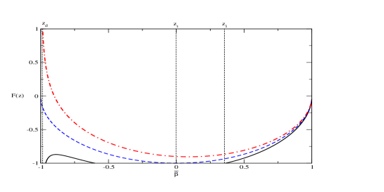
Figure 2: The intervals allowed of $z$: the threshold curve (dashed blue line) with $z_{t}=0$, $\lambda_{t}=2$ and $\overline{\beta}_{t}=0$. Above the threshold, for $\overline{\beta}=\overline{\beta}_{t}+\delta$ (dotted-dashed red line), the dynamics is delocalized since the system can move in the larger interval $[z_{d},1]$, with $z_{d}\approx-0.99$. Below the threshold, $\overline{\beta}=\overline{\beta}_{t}-\delta$ (solid black line), the dynamics is localized since the system is allowed to move in the smaller interval $[z_{l},1]$, with $z_{l}\approx 0.36$. Here we are using $\delta=0.1$.

To find the relationship between the parameters for the threshold curve, we consider $\cos\varphi=\pm 1$, so the above equation becomes

$$\lambda z+(\lambda-2\overline{\beta})=\mp 2\sqrt{\frac{1+z}{1-z}}\equiv g(z).$$ (7)

As the straight line $f(z,\overline{\beta})=\lambda z+(\lambda-2\overline{\beta})$ is tangent to the curve $g(z)$ in some point $z_{t}$, then we have that $\lambda=\frac{\partial g(z)}{\partial z}|_{z=z_{t}}$. Now doing $f(z_{t},\overline{\beta})=g(z_{t})$ we find the threshold coupling point, with the coordinates $\lambda_{t}$ and $\overline{\beta}_{t}$, as a parametric equations of $z_{t}$:

$$\lambda_{t} = \frac{\pm 2}{\sqrt{1+z_{t}}(1-z_{t})^{3/2}},$$

$$\overline{\beta}_{t} = \pm\frac{z_{t}\sqrt{1+z_{t}}}{(1-z_{t})^{3/2}},\qquad z_{t}\in[-\tfrac{1}{2},1).$$ (8)

The above equations gives $z_{t}=\frac{1}{2}\left(\pm\sqrt{\frac{8\overline{\beta}_{t}}{\lambda_{t}}+1}-1\right)$. Clearly there is a minimum point for $\lambda>0$ (maximum point for $\lambda<0$) in the threshold curve. The minimal (maximal) point has coordinates given by

$$\lambda_{m} = \lambda_{t}|_{z_{t}=-1/2}=\pm\frac{8}{3\sqrt{3}}\approx\pm 1.54,$$

$$\bar{\beta}_{m} = -\frac{\lambda_{m}}{8}=\mp\frac{1}{3\sqrt{3}}\approx\mp 0.19.$$

By using eq. (8) we can trace out the threshold curve. These results together with the some solutions of eq. (7) are shown in Fig. 3.

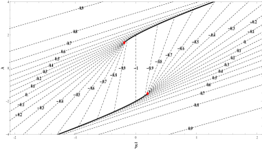
Figure 3: Diagram of coupling parameters $\lambda$ vs $\bar{\beta}$. The threshold curve is represented by the solid black line. The red dot is the mininal (maximal) point for the threshold curve. The dashed lines are obtained from eq. (7) for several values of $z=z_{n}=-0.9+n\,0.2$, $n=0,1,\cdots,9$. Each line represents the values of parameters which determines the interval $[z_{n},1)$ allowed for the classical dynamics.

As there is a symmetry in the diagram of parameter, hereafter we just consider the case $\lambda>0$. For $\lambda>\lambda_{m}$, the threshold curve separates the diagram of parameters in two regions:

• Region I: for $\bar{\beta}<\bar{\beta}_{t}$, the dynamics between wells $1$-$2$ is localized.

• Region II: for $\bar{\beta}>\bar{\beta}_{t}$: the dynanics between wells $1$-$2$ is delocalized;

It is worth to highlight for the case $\lambda>\lambda_{m}$ that the passing through the Region I to the Region II is abrupt configuring the threshold in the classical dynamics. On the other hand side, for $\lambda\leq\lambda_{m}$, there is not a threshold and the classical dynamics changes smoothly. These results are shown in Fig. 4.

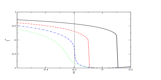
Figure 4: Plot of $z_{max}$ as a function of $\overline{\beta}$, for $\lambda=2.2$ (solid black line), $\lambda=1.8$ (dashed red line), $\lambda=\lambda_{m}$ (dotted-dashed blue line ) and $\lambda=1.3$ (dotted green line). Here $z_{max}=\max Z$, where $Z$ is the set of solutions of equations $F(z)=\pm 1$. The dashed line is $\overline{\beta}=\overline{\beta}_{m}$.

3.2 Classical dynamics

Integrating the above Hamilton’s equations we can see how the classical system is evolving. Recall that $\bar{\beta}=\beta-\omega\lambda$. Thus, if the system is initially in the delocalized dynamics regime (Region II) with $\bar{\beta}>\bar{\beta}_{t}$ and $\lambda>\lambda_{m}$, by increasing the relative population $\omega$, the system will eventually cross the threshold curve to get into the Region I and then the dynamics between wells 1-2 will be localized. In the Fig. 5 we plot the time evolution for $z$ showing the dependence of the parameter $\omega$.

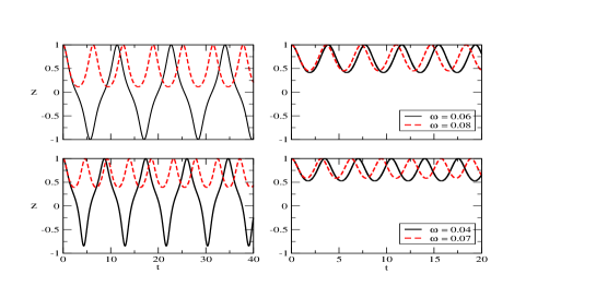
Figure 5: Time evolution for $z$ for two threshold points: above is for the point $P_{1}=(\lambda_{t},\bar{\beta}_{t})=(2,0)$ and below is for the point $P_{2}=(\lambda_{t},\bar{\beta}_{t})=(2.86,0.5)$. On the left side is for $\bar{\beta}=\bar{\beta}_{t}+\delta$ (delocalized region) and on the right is $\bar{\beta}=\bar{\beta}_{t}-\delta$ (localized region). On top the solid line is for $\omega=0.06$ and the dashed line is for $\omega=0.08$ ($\omega_{t}=0.05$). On botton the solid line is for $\omega=0.04$ and the dashed line is for $\omega=0.07$ ($\omega_{t}=0.05$). For the both cases we are using the initial state $(z(0),\varphi(0))=(1-\zeta,0)$,  $\zeta=0.001$, $Q_{1}=100$, $\epsilon=1$ and $\delta=0.1$.

Clearly from Fig. 5 there is a threshold in the classical dynamics when we move from one region to another by varying the parameter $\bar{\beta}$ (solid black line). It is worth noting from Fig. 5 that the increasing of $\omega$ induces always localization on the classical dynamics. The important issue here is to understand that if the system is in a delocalized dynamics regime (Region II) there is a threshold for relative population ($\omega_{t}$) which separates again the dynamics in delocalized and localized regimes. However if the system is in localized dynamics regime (Region I) the dynamics smoothly becomes more localized by increasing the relative population in well $3$ (dashed red line). Next we look if these behaviors are also present in the quantum dynamics of the model.

4 Quantum dynamics

Using the standard procedure now we compute the time evolution of the expectation value of the population imbalance between wells $1$-$2$ using the expression

$$\langle z\rangle=\langle\Psi(t)|\frac{N_{1}-N_{2}}{Q_{1}}|\Psi(t)\rangle,$$ (9)

where $|\Psi(t)\rangle=U(t)|\Psi_{0}\rangle$, $U(t)=e^{-iHt}$ is the temporal evolution operator and $|\Psi_{0}\rangle$ represents the initial state in Fock space. Recall that for fixed value of total number of bosons $N$, the Hilbert space associated to the Hamiltonian (3) has dimension $D=\frac{(N+2)!}{2!N!}$. As $Q_{2}=N_{3}$ is conserved, the Hamiltonian can be written in block-diagonal form for appropriated choice of the basis, where each eigenvalue of $N_{3}$ gives the dimension of each block by $D_{N_{3},N}=N-N_{3}+1$. The total number of blocks is $N+1$, such that $D=\sum_{N_{3}=0}^{N}D_{N_{3},N}$. If one boson is added in the well $3$, then the dimension of Hamiltonian is given by $D=\frac{((N+1)+2)!}{2!(N+1)!}$ and the dimension of block associated to the eigenvalue $N_{3}+1$ is given by $D_{N_{3}+1,N+1}=(N+1)-(N_{3}+1)+1=D_{N_{3},N}$. Therefore, for initial state $|\Psi_{0}\rangle=|N_{1},0,N_{3}\rangle$ the quantum dynamics is just governed by the block with fixed dimension $D_{N_{3},N}=N_{1}+1$ for any $N_{3}\geq 0$.

To start our discussion, firstly, we choose $\beta=\overline{\beta}_{t}\pm\delta$ and $\lambda>\lambda_{m}$ to go from one regime to the another. In Fig. 6 it is shown the time evolution of expectation value of population imbalance $\langle z\rangle$ using four values of $N_{3}$.

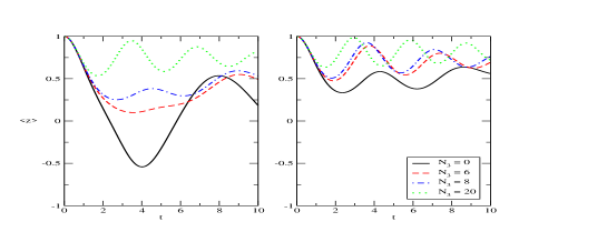
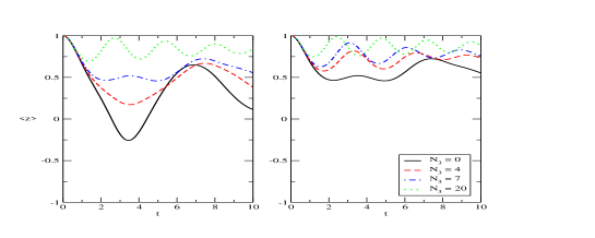
Figure 6: Time evolution of the expectation of population imbalance $\langle z\rangle$ for two threshold points using different values of $\omega$ ($N_{3}$): above is for the point $P_{1}=(\lambda_{t},\bar{\beta}_{t})=(2,0)$ and below is for the point $P_{2}=(\lambda_{t},\bar{\beta}_{t})=(2.86,0.5)$. On the left hand side $\beta=\bar{\beta}_{t}+\delta$ and on the right hand side $\beta=\bar{\beta}_{t}-\delta$. On top: the black solid line if for $N_{3}=0$, the dashed red line is for $N_{3}=6$, the dotted-dashed blue line is for $N_{3}=8$ and the dotted green line is for $N_{3}=20$. On botton: the black solid line if for $N_{3}=0$, the dashed red line is for $N_{3}=4$, the dotted-dashed blue line is for $N_{3}=7$ and the dotted green line is for $N_{3}=20$. In both cases the initial state is $|N_{1},0,N_{3}\rangle$. Here we are using $N_{1}=Q_{1}=100,\;\;\epsilon=1,\;\;\;\delta=0.1$.

In Fig. 6 we choose the initial state $|\Psi_{0}\rangle=|N_{1},0,N_{3}\rangle$ and we observe the time evolution in the localized (right side) and delocalized (left side) regime by changing the population in well $3$. Clearly for both regimes the increasing of population in well $3$ always induces localization of population imbalance between wells $1$-$2$. However in the localized regime (right side) the localization of population imbalance is smooth by increasing the population in well $3$ even around the threshold of the relative population $\omega_{t}$ (see curves for $N_{3}=6,\,8$ ($N_{3}=4,\,7$) on the right hand side of Fig. 6). In the delocalized regime, as predicted classically the dynamics of system will change around $\omega_{t}=\frac{\delta}{\lambda_{t}}$, and a new scenario emerges. A small fraction of bosons putting into well $3$ induces a large localization of population imbalance. In Fig. 7 it is shown the time average $\displaystyle\overline{\langle N_{i}/Q_{1}\rangle}=\frac{1}{\Delta t}\int_{0}^{\Delta t}\langle N_{i}/Q_{1}\rangle dt$,   $i=1,2$, as function of $N_{3}/Q_{1}$, for the interval of time $\Delta t=10$. Clearly we can see the localization effect is more prominent when the relative population is below to $\approx 20\;\%$.

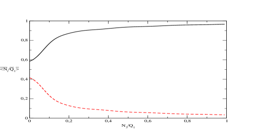
Figure 7: Time average $\overline{\langle N_{1}/Q_{1}\rangle}$ (solid line) and $\overline{\langle N_{2}/Q_{1}\rangle}$ (dashed line), for $\Delta t=10$ against the relative population $\omega=N_{3}/Q_{1}$. Here we are using $N_{1}=100$, $\lambda_{t}=2.0$ and $\overline{\beta}_{t}=0.0$, $\delta=0.1$ and $\epsilon=1$.

Here it is important to observe that around the threshold for the relative population the evolution changes and it has the same pattern that in the localized regime (compare, for example, the dotted-dashed blue line on the left hand side of Fig. 6 with the solid black line on the right hand side of Fig. 6). We highlight that if the system is in the delocalized regime and around the threshold, the dynamics can be driven abruptly from one regime to the another just increasing or decreasing the population in well $3$. This opens the possibility to induce localization or delocalization in the dynamics between wells 1-2 just controlling the population in well $3$ (external control). We believe that this property can be useful to explain quantum devices where the switching scheme is needed.

5 Discussions and overview

The model presented above is the simplest model we can build using three modes and moreover it is integrable in the sense of Bethe ansatz. However, as the apparent simplicity, we believe that this model may be feasible experimentally. Taking into account the extent of the interwell interaction is greater than the range required for tunneling, the results obtained from the model could be verifyed in a proposed experiment using two subtly different possible experimental realization leading to the same physical interpretation:

• spatially bringing closer the well $1$ and well $2$ allowing tunneling between them and then leaving well $3$ at a fixed distance such the tunneling is not allowed but the interwell interactions among them are turned on. By increasing or decreasing the population in well $3$ will change the intensity of the interwell interactions between wells, so in this way we can have control of population imbalance between the wells $1$-$2$ at some distance.

• keeping the population in well $3$ fixed and spatially bringing it closer at the well $1$ and well $2$ and separating apart after an interval of time.

Clearly from our previous theoretical results the variation of the population in well $3$ or analogously the approximation of the well $3$ keeping fixed its population close to the wells $1$-$2$ can be seen as a variation of the intensity of an external field. By the way quantum manipulation via external field is a long-standing research area in physics and chemistry [28, 41]. A study of coherent control of tunneling for an ultracold atoms can be found in the references [42, 43].

On the other hand side, the proposed theoretical model can be seen as the simplest and useful model for modeling quantum devices which needs some control at a distance by using an external field/potential. In this way the model presented here can be useful in atomtronic area [24, 38, 39] since it can mimic a field effect transistor. Taking into account the analogy with the electronic transistor, the well $1$ behaves like the source, the well $2$ behaves like the drain and the well $3$ behaves like the gate. We have demonstrated that tunneling of a large fraction of bosons from well $1$ to well $2$ can be controlled by small fraction of bosons put into the well $3$, without passing through it. In the absence or very small population in well $3$ the device is switched on resulting into the strong flux of bosons from well $1$ (the source) into the well $2$ (the drain). Increasing the population in the well $3$ the flux of bosons from well $1$ to well $2$ becomes smaller and the device starts to be switched off. These results for the model presented in this work is shown in Fig. 8. Here we observe that the transistor-like behavior presented here has a different operation from that transistor-like model presented in reference [24].

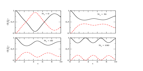
Figure 8: Time evolution of the expectation value of $\langle N_{1}/Q_{1}\rangle$ (solid black line) and $\langle N_{2}/Q_{1}\rangle$ (dashed red line) for the initial state $|\Psi_{0}>=|N_{1},0,N_{3}>$ with different population in well $3$: on the left, top is for $N_{3}=0$ and botton, for $N_{3}=40$; on the right, top is for $N_{3}=30$ and botton, for $N_{3}=100$. Here we are using $\lambda_{t}=2.0$ and $\overline{\beta}_{t}=0.0$, $\delta=0.1$, $\epsilon=1$ and $N_{1}=500$.

Moreover, the proposed model allows us also go further and we can envisioning another interesting scenario. We can induce a change of quantum phase transition by using an external field by controlling the distance between two parallel bidimensional chains. For example, if we are imagining bosons weakly interacting loaded in a bidimensional chain where bosons are in a delocalized dynamics regime with tunneling allowed just on the plane. If another similar bidimensional chain is putting parallel nearby the former one, then taking in account that tunneling between plane is prohibited the change of quantum phase can be induced by changing the interplane distance. That way, we can go from the superfluid-like phase to insulator-like phase just manipulating the interplane separation between bidimensional planes. Our studies are just in the beginning of the investigations and new results will be published somewhere.

6 Conclusions

In summary, in this work we presented the simplest model we can build using three modes and moreover it is integrable in the sense of Bethe ansatz. After, the semiclassical analysis for the model was carried out. The Hamilton’s equations, the diagram of coupling parameters and the classical dynamics were presented. Posteriorly the quantum dynamics of the model was presented and we show that the flow of bosons between the wells $1$-$2$ can be controlled by increasing or decreasing the population in the well $3$ leading to the conclusions that a small population put into well $3$, relative with population in well $1$ and well $2$, generates an effective control of population imbalance between wells $1$-$2$. Later we discussed the experimental feasibility of model suggesting an experiment without taking into account the technicality experimental. In the end, we conclude that the proposed model can be very useful to understand quantum devices which needs a quantum control in its operation, for example, in atomtronic [24, 38, 39, 40] and also in quantum manipulation via external field [28]. Anyway our studies are just beginning and more research in this direction appears to be useful in order to elucidate points and thereby contributing to our understanding of the many-body physics in ultracold bosonic atoms systems.

References

- [1] T.Kinoshita, T. Wenger and D. S. Weiss, Nature 440, 900 (2006)
- [2] M. Rigol, V. Dunjko ans M. Olshanii,Nature 452, 845 (2008)
- [3] J.M. Deutsch, Phys. Rev. A 43, 2046 (1991)
- [4] M. Eckstein, M. Kollar and P. Werner, Phys. Rev. Lett. 103 056403 (2009)
- [5] M.P. Strzys and J.R. Anglin, Phys. Rev. A 81, 043616 (2010)
- [6] D. Manzano and E. Kyoseva, 2016 An atomic symmetry-controlled thermal switch, arXiv:1508.05691v3
- [7] L.D. Faddeev, E.K. Sklyanin and L.A. Takhtajan, Theor. Math. Phys. 40 194 (1979)
- [8] P.P.Kulish and E.K. Sklyanin, Lec. Notes Phys. 151 61(1982)
- [9] L.A. Takhtajan, Lec. Notes Phys. 370 3 (1990)
- [10] L.D. Faddeev, Int. J. Mod. Phys 10 1845 (1995)
- [11] A. J. Leggett, Rev. Mod. Phys. 73 (2001), 307
- [12] G. J. Milburn, J. Corney, E. M. Wright and D. F. Walls, Phys. Rev. A 55 4318 (1997)
- [13] J.Links, A. Foerster, A. Tonel and G. Santos, Ann. Henri Poincaré 7 1591 (2006)
- [14] A.P. Tonel, J. Links, A. Foerster, J. Phys. A: Math. Gen. 38 1235 (2005)
- [15] A.P. Tonel, J. Links, A. Foerster, J. Phys. A: Math. Gen. 38 6879 (2005)
- [16] J. Williams, R. Walser, J. Cooper, E. A. Cornell and M. Holland Phys. Rev. A 61 033612 (2000)
- [17] M. Albiez, R. Gati, J. Folling, S. Hunsmann, M. Cristiani and M. K. Oberthaler, Phys. Rev. Lett. 95 010402 (2005)
- [18] K. Nemoto, C. A. Holmes, G.J. Milburn and W.J. Munro, Phys. Rev. A 63 013604 (2000)
- [19] T. Lahaye, T. Pfau and L. Santos,Phys.Rev.Lett. 104 170404 (2010)
- [20] A. Gallemi, M. Guilleumas, R. Mayol and A. Sanpera, Phys. Rev. A 88 063645 (2013)
- [21] D. Peter, K. Pawlowski, T. Pfau and K. Rzazewski,J. Phys. B: At. Mol. Opt. Phys. 45 225302 (2012)
- [22] J-M. Liu and Y-Z. Wang, Int. J. Mod. Phys. B 20 277 (2006)
- [23] F. Wang, X. Yan and D. Wang, Int. J. Mod. Phys. B 23 383 (2009)
- [24] J.A. Stickney, D. Z. Anderson and A. A. Zozulya , Phys. Rev. A 75 013608 (2007)
- [25] C.V. Chianca and M.K. Olsen, Phys.Rev. A 83, 043607 (2011)
- [26] S. De Liberato and C. J. Foot, Phys.Rev. A 73, 035602 (2006)
- [27] I. Zerec, V. Keppens, M.A. McGuire, D. Mandrus, B.C. Sales and P. Thalmeier Phys. Rev. Lett. 92, 185502 (2004)
- [28] G. Lu, W. Hai and M. Zou, J. Phys. B: At. Mol. Opt. Phys. 45, 185504 (2012)
- [29] G. Mazzarella and V. Penna, J. Phys. B: At. Mol. Opt. Phys. 48, 065001 (2015)
- [30] P. Schlagheck and J. Dujardin, Coherent backscattering in the Fock space of ultracold bosonic atoms, arXiv:1610.04350v1
- [31] Q. Zhou and S. Das Sarma, Phys. Rev. A 82 041601 (2010)
- [32] A-X. Zhang, S-L. Tian,R-A. Tang and J-K. Xue, Chin. Phys. Lett. 25, 3566 (2008)
- [33] A.P. Tonel, L.H. Ymai, A. Foerster and J. Links, J. Phys. A: Math. Theor. 48, 494001(2015)
- [34] L.H. Ymai, A.P. Tonel, A. Foerster and J. Links, 2016 Quantum integrable multi-well tunneling models, arXiv:1606.00816
- [35] G. Santos, A. Foerster, I. Roditi, J. Phys. A: Math. Theor. 46, 265206 (2013)
- [36] G. Santos, The exact solution of a generalized Bose–Hubbard model, arXiv:1605.08452v1
- [37] A.P. Tonel, L.H. Ymai, K. Wilsmann, J. Links and A. Foerster, in preparation (2016)
- [38] B.T. Seaman, M. Kramer, D.Z. Anderson and M.J. Holland, Phys. Rev. A 75 023615 (2007)
- [39] J.A. Stickney, D.Z. Anderson and A.A. Zozulya, Phys. Rev. A 75 013608 (2007)
- [40] S. Moulder, S. Beattie, R.P. Smith, N. Tammuz and Z. Hadzibabic, Phys. Rev. A 86 013629 (2012)
- [41] H. Rabitz, R. de Vivie-Riedle, M. Motzkus and K. Kompa Science 288 824 (2000)
- [42] E. Kierig, U. Schnorrberger, A. Schietinger, J. Tomkovic, and M. K. Oberthaler Phys. Rev. Lett. 100 190405 (2008)
- [43] G. Lu, W. Hai and H. Zhong, Phys. Rev. A 80 013411 (2009)