Gibbs Measures with memory of length 2 on an arbitrary order Cayley tree

Abstract.

In this paper, we consider the Ising-Vanniminus model on an arbitrary order Cayley tree. We generalize the results conjectured in [3, 4] for an arbitrary order Cayley tree. We establish existence and a full classification of translation invariant Gibbs measures with memory of length 2 associated with the model on arbitrary order Cayley tree. We construct the recurrence equations corresponding generalized ANNNI model. We satisfy the Kolmogorov consistency condition. We propose a rigorous measure-theoretical approach to investigate the Gibbs measures with memory of length 2 for the model. We explain whether the number of branches of tree does not change the number of Gibbs measures. Also we take up with trying to determine when phase transition does occur.

Keywords: Solvable lattice models, Rigorous results in statistical mechanics, Gibbs measures, Ising-Vannimenus model, phase transition.
PACS: 05.70.Fh; 05.70.Ce; 75.10.Hk.

1. Introduction

One of the main purposes of equilibrium statistical mechanics consists in describing all limit Gibbs distributions corresponding to a given Hamiltonian [9]. One of the methods used for the description of Gibbs measures on Cayley trees is Markov random field theory and recurrent equations of this theory [27, 28, 30, 33, 35, 38, 40]. The approach we use here is based on the theory of Markov random fields on trees and recurrent equations of this theory. In this paper, we discuss their relation with the recurrent equations of the theory of Markov random fields on trees for Ising model [28, 32]. In [22], we obtain a new set of limiting Gibbs measures for the Ising model on a Cayley tree. In [2, 17, 18], the authors study the phase diagram for the Ising model on a Cayley tree of arbitrary order $k$ with competing interactions. In [18], the authors characterized each phase by a particular attractor and the obtained the phase diagram by following the evolution and detecting the qualitative changements of these attractors.

$n$-dimensional integer lattice, denoted $\mathbf{Z}^{n}$, has so-called amenability property. Moreover, analytical solutions does not exist on such lattice. But investigations of phase transitions of spin models on hierarchical lattices showed that there are exact calculations of various physical quantities (see for example, [23, 35]). Such studies on the hierarchical lattices begun with the development of the Migdal-Kadanoff renormalization group method where the lattices emerged as approximants of the ordinary crystal ones. On the other hand, the study of exactly solved models deserves some general interest in statistical mechanics [31].

A Cayley tree is the simplest hierarchical lattice with non-amenable graph structure [26]. Also, Cayley trees still play an important role as prototypes of graphs [7]. This means that the ratio of the number of boundary sites to the number of interior sites of the Cayley tree tends to a nonzero constant in the thermodynamic limit of a large system. Nevertheless, the Cayley tree is not a realistic lattice, however, its amazing topology makes the exact calculations of various quantities possible.

One of the most interesting problems in statistical mechanics on a lattice is the phase transition problem, i.e. deciding whether there are many different Gibbs measures associated to a given Hamiltonian [10, 11, 29, 40]. Investigations of phase transitions of spin models on hierarchical lattices showed that they make the exact calculation of various physical quantities [34, 36, 37]. It was established the existence of the phase transition, for the model in terms of finitely correlated states, which describes ground states of the model. Up to this day many authors have studied the existence of phase transition by means of the recurrence equations corresponding to the Ising-Vanniminus model on Cayley tree of order two and three [3, 4, 22, 28, 33]. Recently, Ganikhodjaev [29] has studied the existence of phase transition for Ising model on the semi-infinite Cayley tree of second order with competing interactions up to third-nearest-neighbor generation with spins belonging to the different branches of the tree. In the present paper, for a given Hamiltonian, we provide a more general construction of Gibb measures associated with the Hamiltonian. We prove the existence of translation-invariant Gibb measures associated to the model which yield the existence of the phase transition.

It is well known that the Potts model is a generalization of the Ising model, but the Potts model on a Cayley tree is not well studied, compared to the Ising model [35]. In the last decade, many researches have investigated Gibbs measures associated with Potts model on Cayley trees [12, 13, 14, 15, 16, 27]. In [13], we studied the existence, uniqueness and non-uniqueness of the Gibbs measures associated with the Potts model on a Bethe lattice of order three with three coupling constants by using Markov random field method. In [14], we have obtained the exact solution of a phase transition problem by means of Gibbs state of the same Potts model in [14].

In the present paper, we are concerned with the Ising-Vanniminus model on an arbitrary order Cayley tree. We investigate translation invariant Gibbs measures associated with Ising-Vannimenus model on arbitrary order Cayley tree. We generalize the results obtained in [3, 4]. We use the Markov random field method to describe the Gibbs measures. We satisfy the Kolmogorov consistency condition. We propose a rigorous measure-theoretical approach to investigate the Gibbs measures with memory of length 2 corresponding to the Ising-Vanniminus model on a Cayley tree of arbitrary order. Also we take up with trying to determine when phase transition does occur.

The outline of this paper is as follows. In Section 2 we give the definitions of the Cayley tree, Gibbs measures and Ising-Vannimenus model. Section 3 provides a construction of Gibbs measures on an arbitrary order Cayley tree. In Section 4 we establish the existence, uniqueness and non-uniqueness of the translation-invariant Gibbs measures by means of the recurrence equations for $k$-even, while in Section 5 we do the same for $k$-odd. We contain in Section 6 concluding remarks and discussion of the consequences of the results with next problems.

2. PRELIMINARIES

2.1. Cayley trees

Cayley trees (or Bethe lattices) are simple connected undirected graphs $G=(V,E)$ ($V$ set of vertices, $E$ set of edges) with no cycles (a cycle is a closed path of different edges), i.e., they are trees [7]. Let $\Gamma^{k}=(V,L,i)$ be the uniform Cayley tree of order $k$ with a root vertex $x^{(0)}\in V$, where each vertex has $k+1$ neighbors with $V$ as the set of vertices and the set of edges. The notation $i$ represents the incidence function corresponding to each edge $\ell\in L$, with end points $x_{1},x_{2}\in V$. There is a distance $d(x,y)$ on $V$ the length of the minimal point from $x$ to $y$, with the assumed length of 1 for any edge (see Figure 1).

We denote the sphere of radius $n$ on $V$ by $W_{n}=\{x\in V:d(x,x^{(0)})=n\}$ and the ball of radius $n$ by $V_{n}=\{x\in V:d(x,x^{(0)})\leq n\}.$ The set of direct successors of any vertex $x\in W_{n}$ is denoted by $S_{k}(x)=\{y\in W_{n+1}:d(x,y)=1\}.$

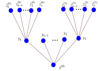
Figure 1. Two successive generations of semi-infinite Cayley tree $\Gamma^{k}$ of arbitrary order $k>1$ (branching ratio is finite $k$). The fixed vertex $x^{(0)}$ is the root of the lattice that emanates $k$ edges of $\Gamma^{k}$ ($y_{j}\in S(x^{(0)}),z_{i}^{(j)}\in S(y_{j})$).

2.2. Ising-Vannimenus model

The Ising model with competing nearest-neighbors interactions is defined by the Hamiltonian

$$H(\sigma)=-J\sum_{<x,y>\subset V}\sigma(x)\sigma(y),$$ (2.1)

where the sum runs over nearest-neighbor vertices $<x,y>$ and the spins $\sigma(x)$ and $\sigma(y)$ take values in the set $\Phi=\{-1,+1\}$.

The Hamiltonian

$$H(\sigma)=-J_{p}\sum_{>x,y<}\sigma(x)\sigma(y)-J\sum_{<x,y>}\sigma(x)\sigma(y)$$ (2.2)

defines the Ising-Vannimenus model with competing nearest-neighbors and next-nearest-neighbors, with the sum in the first term representing the ranges of all nearest-neighbors, where $J_{p},J\in\mathbb{R}$ are coupling constants corresponding to prolonged next-nearest-neighbor and nearest-neighbor potentials [21].

2.3. Gibbs measures

A finite-dimensional distribution of measure $\mu$ in the volume $V_{n}$ has been defined by formula

$$\mu_{n}(\sigma_{n})=\frac{1}{Z_{n}}\exp[-\frac{1}{T}H_{n}(\sigma)+\sum_{x\in W_{n}}\sigma(x)h_{x}]$$ (2.3)

with the associated partition function defined as

$$Z_{n}=\sum_{\sigma_{n}\in\Phi^{V_{n}}}\exp[-\frac{1}{T}H_{n}(\sigma)+\sum_{x\in W_{n}}\sigma(x)h_{x}],$$

where the spin configurations $\sigma_{n}$ belongs to $\Phi^{V_{n}}$ and $h=\{h_{x}\in\mathbb{R},x\in V\}$ is a collection of real numbers that define boundary condition (see [11, 36, 37]). Physically, Eq. (2.3) represents the first step of the Bethe-Peierls approach [8]. Bleher [1] proved that the disordered Gibbs distribution (2.3) in the ferromagnetic Ising model associated to the Hamiltonian (2.1) on the Cayley tree is extreme for $T\geq T^{SG}_{C}$, where $T^{SG}_{C}$ is the critical temperature of the spin glass model on the Cayley tree, and it is not extreme for $T<T^{SG}_{C}$. Previously, researchers frequently used memory of length 1 over a Cayley tree to study Gibbs measures [11, 36, 37].

Let $S=\{1,2,...,s\}$ be a finite state space. On the infinite product space ${{S}^{\mathbb{Z}}}$, one can define the product $\sigma$-algebra, which is generated by cylinder sets ${}_{m}[i_{1},...,i_{N}]$ of length $N$ based on the block $(i_{1},...,i_{N})$ at the place $m$. We denote by ${{\mathfrak{M}}}({{S}^{\mathbb{Z}}})$ the set of all measures on ${{S}^{\mathbb{Z}}}$. The set of all $\sigma$-invariant measures in ${{S}^{\mathbb{Z}}}$ is denoted by ${{\mathfrak{M}}_{\sigma}}({{S}^{\mathbb{Z}}})$, where $\sigma$ is the shift transformation.

Proposition 2.1.

[5, (8.1) Proposition] For $\mu\in{{\mathfrak{M}}_{\sigma}}({{S}^{\mathbb{Z}}})$ the following properties are valid:

1. $\sum\limits_{i\in S}{\mu{{(}_{0}}[i])=1}$;

2. $\mu(_{n}[i_{0},...,i_{k}])\geq 0$ for any block $({{i}_{0}},{{i}_{1}},...,{{i}_{k}})\in S^{k+1}$ and any $n\in\mathbb{Z}$;

3. $\mu(_{n}[{{i}_{0}},...,{{i}_{k}}])=\sum\limits_{{{i}_{k+1}}\in S}{\mu{{(}_{n}}[{{i}_{0}},...,{{i}_{k}},{{i}_{k+1}}])}$;

4. $\mu(_{n}[{{i}_{0}},...,{{i}_{k}}])=\sum\limits_{{{i}_{-1}}\in S}{\mu{{(}_{n}}[{{i}_{-1}},{{i}_{0}},...,{{i}_{k}}])}$.

The proof of the Proposition 2.1 can clearly be checked for both the Bernoulli and the Markov measures on $\sigma$-algebra [5]. By a special case of Kolmogoroff’s consistency theorem (see [5]), these properties are sufficient to define a measure. It is well known that a Gibbs measure is a generalization of a Markov measure to any graph, therefore any Gibbs measure should satisfy the conditions in the Proposition 2.1. In the next sections, we will show that the Gibbs measure associated to the Ising-Vannimenus model satisfies the conditions in the Proposition 2.1.

Let us consider increasing subsets of the set of states for one dimensional lattices [25] as follows:

$$\mathfrak{G}_{1}\subset\mathfrak{G}_{2}\subset...\subset\mathfrak{G}_{n}\subset...,$$

where $\mathfrak{G}_{n}$ is the set of states corresponding to non-trivial correlations between $n$-successive lattice points; $\mathfrak{G}_{1}$ is the set of mean field states; and $\mathfrak{G}_{2}$ is the set of Bethe-Peierls states, the latter extending to the so-called Bethe lattices. All these states correspond in probability theory to so-called Markov chains with memory of length $n$ (see [24, 25, 31]).

In [25], by using the idea of Bayesian extension, Fannes and Verbeure defined states known as a finite-block measure or as Markov chains with memory of length $n$ on the lattices. Recently, the author has studied the Gibbs measures with memory of length 2 associated to the Ising-Vannimenus model on the Cayley tree of order two and three [3, 4]. The construction is based on the idea in the Proposition 2.1. In the present paper, we are going to establish the existence of Gibbs measures associated with the Ising-Vannimenus model with memory of length 2 on the Cayley tree of arbitrary order.

3. Construction of Gibbs measures on Cayley tree

In this section, we will presents the general structure of Gibbs measures with memory of length 2 associated with the Hamiltonian (2.2) on an arbitrary order Cayley tree. On non-amenable graphs, Gibbs measures depend on boundary conditions [35]. This paper considers this dependency for Cayley trees, the simplest of graphs.

An arbitrary edge $<x^{(0)},x^{(1)}>=\ell\in L$ deleted from a Cayley tree $\Gamma_{1}^{k}$ and $\Gamma_{0}^{k}$ splits into two components: semi-infinite Cayley tree $\Gamma_{1}^{k}$ and semi-infinite Cayley tree $\Gamma_{0}^{k}$. This paper considers a semi-infinite Cayley tree $\Gamma_{0}^{k}$. For a finite subset $V_{n}$ of the lattice, we define the finite-dimensional Gibbs probability distributions on the configuration space $\Omega^{V_{n}}=\{\sigma_{n}=\{\sigma(x)=\pm 1,x\in V_{n}\}\}$ at inverse temperature $\beta=\frac{1}{kT}$ by formula.

Let $x\in W_{n}$ for some $n$ and $S(x)=\{{{y}_{1}},{{y}_{2}},\cdots,{{y}_{k}}\}$ are the direct successors of $x$, where ${{y}_{1}},{{y}_{2}},\cdots,{{y}_{k}}\in{{W}_{n+1}}$.

Denote ${{B}_{1}}(x)=\left(\begin{matrix}{{y}_{k}},\cdots,{{y}_{2}},{{y}_{1}}\\ x\\ \end{matrix}\right)$ a unite semi-ball with a center $x$. We denote the set of all spin configurations on $V_{n}$ by $\Phi^{V_{n}}$ and the set of all configurations on unite semi-ball $B_{1}(x)$ by $\Phi^{B_{1}(x)}$. One can get that the set $\Phi^{B_{1}(x)}$ consists of ${{2}^{k+1}}$ configurations:

$$\Phi^{B_{1}(x)}=\left\{\left(\begin{matrix}i_{k},\cdots,i_{2},i_{1}\\ i\\ \end{matrix}\right):i,i_{1},i_{2},\cdots,i_{k}\in\Phi\right\}.$$

Let

$$\sigma_{S}({{x}^{(0)}})=\left(\begin{matrix}\sigma({{y}_{k}}),\cdots,\sigma({{y}_{2}}),\sigma({{y}_{1}})\\ \sigma({{x}^{(0)}})\\ \end{matrix}\right)$$

be a configuration on the set ${{x}^{(0)}}\cup S({{x}^{(0)}})$ and

$$\sigma_{S}({{y}_{i}})=\left(\begin{matrix}\sigma(z_{k}^{(i)}),\cdots,\sigma(z_{2}^{(i)}),\sigma(z_{1}^{(i)})\\ \sigma({{y}_{i}})\\ \end{matrix}\right)$$

be a configuration on the set ${{y}_{i}}\cup S({{y}_{i}}),$ ${y}_{i}\in S({{x}^{(0)}})$. Let $\Omega(S)$ be the set of all such configurations.

We wish to consider a probability measure $\mu_{\mathbf{h}}^{(n)}$ that is formally given by

$$\mu_{\mathbf{h}}^{(n)}(\sigma)=\frac{1}{Z_{\mathbf{h}}^{(n)}}\exp[-\beta{{H}_{n}}(\sigma)+\sum\limits_{x\in{{W}_{n-1}}}{\sum\limits_{y\in S(x)}{\sigma}}(x)\prod\limits_{y\in S(x)}{\sigma(y)h_{B_{1}(y);\sigma_{S}(y)}}],$$ (3.1)

where $\beta=\frac{1}{{{k}_{B}}T}$, ${{k}_{B}}$ is the Boltzmann constant and $h_{B_{1}(y);\sigma_{S}(y)}$ is a real-valued function of $y\in V$. $\sigma_{n}:x\in V_{n}\to\sigma_{n}(x)$ and $Z_{\mathbf{h}}^{(n)}$ corresponds to the following partition function:

$$Z_{\mathbf{h}}^{(n)}=\sum\limits_{{{\sigma}_{n}}\in{{\Phi}^{{{V}_{n}}}}}{\exp}[-\beta H({{\sigma}_{n}})+\sum\limits_{x\in{{W}_{n-1}}}{\sum\limits_{y\in S(x)}{\sigma}}(x)\prod\limits_{y\in S(x)}{\sigma(y){{h}_{B_{1}(y);\sigma_{S}(y)}}}].$$ (3.2)

In this paper, we suppose that vector valued function $\textbf{h}:V\rightarrow\mathbb{R}^{2(k+1)}$ is defined by

$$\textbf{h}:(x,y_{k},y_{k-1},\ldots,y_{2},y_{1})\rightarrow\textbf{h}_{B_{1}(x)}=(h_{B_{1}(x);\sigma_{S}({{x}})}:y_{i}\in S(x)),$$ (3.3)

where $h_{B_{1}(x);\sigma_{S}({{x}})}\in\mathbb{R}$, $x\in W_{n-1}$ and $y_{i}\in S(x).$

We will consider a construction of an infinite volume distribution with given finite-dimensional distributions. More exactly, we will attempt to find a probability measure $\mu$ on $\Omega$ that is compatible with given measures $\mu_{\textbf{h}}^{(n)}$, i.e.,

$$\mu(\sigma\in\Omega:\sigma|_{V_{n}}=\sigma_{n})=\mu^{(n)}_{\textbf{h}}(\sigma_{n}),\ \ \ \textrm{for all}\ \ \sigma_{n}\in\Omega^{V_{n}},\ n\in\mathbf{N}.$$ (3.4)

We say that the probability distributions $\mu_{\textbf{h}}^{n}$ satisfy the Kolmogorov consistency condition if for any configuration $\sigma_{n-1}\in\Omega^{V_{n-1}}$

$$\sum_{\omega\in\Omega^{W_{n}}}\mu^{(n)}_{\textbf{h}}(\sigma_{n-1}\vee\omega)=\mu^{(n-1)}_{\textbf{h}}(\sigma_{n-1}).$$ (3.5)

This condition implies the existence of a unique measure $\mu_{\textbf{h}}^{(n)}$ defined on $\Omega$ with a required condition (3.4). Such a measure $\mu_{\textbf{h}}^{(n)}$ is called a Gibbs measure with memory of length 2 associated to the model (2.2).

We note that first two conditions of Proposition 2.1 is trivial to check for the measure in (3.1). The condition (3) of Proposition 2.1 is the same as the condition in (3.5). Therefore, it should be proved that the Gibbs measure (3.1) satisfies the condition (3) in the Proposition 2.1.

4. The recurrence equations for $k$-even

Let $k$ be the positive even integer, where $k$ is the order of the Cayley tree. It is reasonable, though, to assume that the different branches are equivalent, as is usually done for models on trees.

Let

$$\sigma_{S}^{+}({{x}^{(0)}})=\left(\begin{matrix}\sigma({{y}_{k}}),\cdots,\sigma({{y}_{2}}),\sigma({{y}_{1}})\\ +\\ \end{matrix}\right)$$

be a configuration in $\Phi^{B_{1}(x)}$ (see Fig. 1). Let $m$ be the number of spins down, i.e., $\sigma({{y}_{i}})=-1$ on the first level ${{W}_{1}}$, where $0\leq m\leq k$. Then $(k-m)$ is the number of spins up, i.e., $\sigma({{y}_{i}})=+1$ on the first level ${{W}_{1}}$. Let

$$\sigma_{S}^{+}({{y}_{i}})=\left(\begin{matrix}\sigma(z_{k}^{(i)}),\cdots,\sigma(z_{2}^{(i)}),\sigma(z_{1}^{(i)})\\ +\\ \end{matrix}\right)$$

be a configuration in $\Omega(S)$. Let $m$ be the number of spins down, i.e., $\sigma(z_{j}^{(i)})=-1$ on the second level ${{W}_{2}}$, where $0\leq m\leq k.$ Let

$$\sigma_{S}^{-}({{x}^{(0)}})=\left(\begin{matrix}\sigma({{y}_{k}}),\cdots,\sigma({{y}_{2}}),\sigma({{y}_{1}})\\ -\\ \end{matrix}\right)$$

be a configuration in $\Omega(S)$. Let $m$ be the number of spins down, i.e., $\sigma(y_{i})=-1$ on the first level ${{W}_{1}}$, where $0\leq m\leq k.$ Let

$$\sigma_{S}^{-}({{y}_{i}})=\left(\begin{matrix}\sigma(z_{k}^{(i)}),\cdots,\sigma(z_{2}^{(i)}),\sigma(z_{1}^{(i)})\\ -\\ \end{matrix}\right)$$

be a configuration in $\Omega(S)$ (see Fig. 1). Let $m$ be the number of spins down, i.e., $\sigma(z_{j}^{(i)})=-1$ on the second level ${{W}_{2}}$, where $0\leq m\leq k.$

For clarity, denote the configuration of the set $\Phi^{B_{1}(x^{(0)})}$ by

$$S_{m}^{(k-m)}(\sigma({{x}^{(0)}}))=\left(\begin{matrix}\overbrace{++\cdots+}^{k-m}\overbrace{--\cdots-}^{m}\\ \sigma(x^{(0)})\\ \end{matrix}\right).$$

From the consistency condition (3.5), we can use the following equation:

Theorem 4.1.

[3] The measures $\mu_{{\mathbf{h}}}^{(n)}(\sigma)$, $n=1,2,...,$ in (2.3) satisfy the compatibility condition (3.5) if and only if for any $n\in\mathbf{N}$ the following equations hold:

$$\exp(h_{B_{1}(x^{(0)});S_{0}^{k}(+)}+h_{B_{1}(x^{(0)});S_{0}^{k}(-)}) = \frac{\left(\sum\limits_{i=0}^{k}\left(\begin{array}[]{c}k\\ i\end{array}\right)(ab)^{k-2i}(-1)^{i}{{h}_{{{B}_{1}}(y_{i});S_{i}^{k-i}(+)}}\right)^{k}}{{{\left(\sum\limits_{i=0}^{k}{\left(\begin{array}[]{c}k\\ i\end{array}\right){{\left(\frac{a}{b}\right)}^{k-2i}}}(-1)^{i}{{h}_{{{B}_{1}}(y_{i});S_{i}^{k-i}(+)}}\right)}^{k}}}$$

$$\exp(h_{B_{1}(x^{(0)});S_{0}^{k}(+)}+h_{B_{1}(x^{(0)});S_{k}^{0}(-)}) = \frac{\left(\sum\limits_{i=0}^{k}\left(\begin{array}[]{c}k\\ i\end{array}\right)(ab)^{k-2i}(-1)^{i}{{h}_{{{B}_{1}}(y_{i});S_{i}^{k-i}(+)}}\right)^{k}}{\left(\sum\limits_{i=0}^{k}\left(\begin{array}[]{c}k\\ i\end{array}\right)(ab)^{2i-k}{{(-1)}^{i+1}}{{h}_{{{B}_{1}}(y_{i});S_{i}^{k-i}(-)}}\right)^{k}}$$

$$\exp(h_{B_{1}(x^{(0)});S_{k}^{0}(+)}+h_{B_{1}(x^{(0)});S_{k}^{0}(-)}) = \frac{\left(\sum\limits_{i=0}^{k}\left(\begin{array}[]{c}k\\ i\\ \end{array}\right)\left(\frac{b}{a}\right)^{k-2i}{{(-1)}^{i+1}}{{h}_{{{B}_{1}}(y_{i});S_{i}^{k-i}(-)}}\right)^{k}}{\left(\sum\limits_{i=0}^{k}\left(\begin{array}[]{c}k\\ i\end{array}\right)(ab)^{2i-k}{{(-1)}^{i+1}}{{h}_{{{B}_{1}}(y_{i});S_{i}^{k-i}(-)}}\right)^{k}}$$

where $a=e^{\beta J}$ and $b=e^{\beta J_{p}}$.

The Theorem 4.1 partially confirms the conjecture formulated in [3]. Also, the proof of the Theorem 4.1 can be done as similar to [3].

By means of the last equalities, from (3.1) and (3.2) we can get that

$$\exp(\sigma(x^{(0)})\prod_{y\in S(x^{(0)})}\sigma(y)h_{B_{1}(x^{(0)});S_{m}^{k-m}(\sigma(x^{(0)}))})$$

$$= L_{2}\sum_{\eta\in\Phi^{W_{2}}}(\exp(\beta J\sum_{y_{i}\in S(x^{(0)})}\sigma(y_{i})\sum_{z_{j}^{(i)}\in S(y_{i})}\eta(z_{j}^{(i)}))$$

$$\times\exp(\beta J_{p}\sigma(x^{(0)})\sum_{z_{j}^{(i)}\in S^{2}(x^{(0)})}\eta(z_{j}^{(i)})+\sum_{y_{i}\in S(x^{(0)})}\sigma(y_{i})\prod_{z_{j}^{(i)}\in S(y_{i})}\eta(z_{j}^{(i)})h_{B_{1}(y_{i});S_{m}^{k-m}(\sigma(y_{i}))}))$$

where ${{L}_{2}}=\frac{{{Z}_{1}}}{{{Z}_{2}}}.$

Consider the configuration $S_{0}^{k}(\sigma({{x}^{(0)}})=+)=\left(\begin{matrix}+,\cdots,+,+\\ +\\ \end{matrix}\right)$. For the sake of simplicity, assume such that $\exp[(-1)^{m}{{h}_{{{B}_{1}}(y_{i});S_{m}^{k-m}(\sigma(y)=+1)}}]=u_{1+m}^{{{(-1)}^{m}}}$, we have

$$u_{1}^{{}^{\prime}}=\exp(h_{B_{1}(x^{(0)});S_{0}^{k}(+)})=L_{2}\left(\sum\limits_{i=0}^{k}\left(\begin{array}[]{c}k\\ i\end{array}\right)(ab)^{-2i+k}u_{1+i}^{{{(-1)}^{i}}}\right)^{k}.$$ (4.7)

Now let us consider the configuration $S_{k}^{0}(\sigma({{x}^{(0)}})=+)=\left(\begin{matrix}-,\cdots,-,-\\ +\\ \end{matrix}\right)$ and let

$$\exp[{{(-1)}^{m+1}}{{h}_{{{B}_{1}}(y_{i});S_{m}^{k-m}(\sigma(y_{i})=-1)}}]=u_{k+2+m}^{{{(-1)}^{m+1}}},$$

then we have

$$u_{k+1}^{{}^{\prime}}=\exp(h_{B_{1}(x^{(0)});S_{k}^{0}(+)})=L_{2}\left(\sum\limits_{i=0}^{k}\left(\begin{array}[]{c}k\\ i\\ \end{array}\right)\left(\frac{b}{a}\right)^{-2i+k}u_{2+i+k}^{{(-1)}^{1+i}}\right)^{k}.$$ (4.10)

Similarly, for the configuration $S_{0}^{k}(\sigma({{x}^{(0)}})=-)=\left(\begin{matrix}+,\cdots,+,+\\ -\\ \end{matrix}\right)$, one can obtain

$${{\left(u_{k+2}^{{}^{\prime}}\right)}^{-1}}=\exp(-h_{B_{1}(x^{(0)});S_{0}^{k}(-)})={{L}_{2}}{{\left(\sum\limits_{i=0}^{k}{\left(\begin{array}[]{c}k\\ i\end{array}\right){{\left(\frac{a}{b}\right)}^{-2i+k}}}u_{1+i}^{{{(-1)}^{i}}}\right)}^{k}}.$$ (4.13)

Lastly, for the configuration $S_{k}^{0}(\sigma({{x}^{(0)}})=-)=\left(\begin{matrix}-,\cdots,-,-\\ -\\ \end{matrix}\right)$ we have

$${{\left(u_{2(k+1)}^{{}^{\prime}}\right)}^{-1}}=\exp(-h_{B_{1}(x^{(0)});S_{k}^{0}(-)})=L_{2}\left(\sum\limits_{i=0}^{k}\left(\begin{array}[]{c}k\\ i\end{array}\right)(ab)^{2i-k}u_{2+i+k}^{(-1)^{1+i}}\right)^{k}.$$ (4.16)

From (4.7)-(4.16) we immediately get that

$$e^{(-1)^{m}h_{B_{1}(x^{(0)});S_{m}^{k-m}(+)}} = \left(e^{h_{B_{1}(x^{(0)});S_{0}^{k}(+)}}\right)^{\frac{k-m}{k}}\left(e^{h_{B_{1}(x^{(0)});S_{k}^{0}(+)}}\right)^{\frac{m}{k}}$$ (4.17)

$$e^{(-1)^{m+1}h_{B_{1}(x^{(0)});S_{m}^{k-m}(-)}} = \left(e^{-h_{B_{1}(x^{(0)});S_{0}^{k}(-)}}\right)^{\frac{k-m}{k}}\left(e^{-h_{B_{1}(x^{(0)});S_{k}^{0}(-)}}\right)^{\frac{m}{k}}.$$ (4.18)

Through the introduction of the new variables $v_{i}=(u_{i})^{\frac{1}{k}}$ in the equations (4.7)-(4.18), we derive the following recurrence system:

$$v_{1}^{{}^{\prime}} = \sqrt[k]{L_{2}}{{\left(\frac{{{(ab)}^{2}}{{v}_{1}}+{{v}_{k+1}}}{ab}\right)}^{k}},$$ (4.19)

$$v_{k+1}^{{}^{\prime}} = \sqrt[k]{L_{2}}{{\left(\frac{{{a}^{2}}{{v}_{k+2}}+{{b}^{2}}{{v}_{2(k+1)}}}{ab{{v}_{k+2}}{{v}_{2(k+1)}}}\right)}^{k}},$$ (4.20)

$$(v_{k+2}^{{}^{\prime}})^{-1} = \sqrt[k]{L_{2}}{{\left(\frac{{{a}^{2}}{{v}_{1}}+{{b}^{2}}{{v}_{k+1}}}{ab}\right)}^{k}},$$ (4.21)

$$(v_{2(k+1)}^{{}^{\prime}})^{-1} = \sqrt[k]{L_{2}}{{\left(\frac{{{(ab)}^{2}}{{v}_{k+2}}+{{v}_{2(k+1)}}}{(ab){{v}_{k+2}}{{v}_{2(k+1)}}}\right)}^{k}}.$$ (4.22)

4.1. Translation-invariant Gibbs measures: Even case

In this subsection, we are going to focus on the existence of translation-invariant Gibbs measures (TIGMs) by analyzing the equations (4.19)-(4.22). Note that vector-valued function

$$\textbf{h}(x)=\{h_{B_{1}(x);S_{m}^{k-m}(\sigma(x))}:m\in\{0,1,2,...,k\},\sigma(x)\in\Phi\}$$ (4.23)

is considered as translation-invariant if $h_{B_{1}(x);S_{m}^{k-m}(\sigma(x))}=h_{B_{1}(y);S_{m}^{k-m}(\sigma(y))}$ for all $y\in S(x)$ and $\sigma(x)=\sigma(y)$ (see for details [3, 35]). A translation-invariant Gibbs measure is defined as a measure, $\mu_{\textbf{h}}$, corresponding to a translation-invariant function h (see for details [28, 35]). Here we will assume that $v^{\prime}_{i}=v_{i}$ for all $i\in\{1,\ldots,2(k+1)\}$.

Remark 4.1.

By using the equations (4.17) and (4.18), it can be shown that if the vector-valued function $\textbf{h}(x)$ given in (4.23) has the following form:

$$\textbf{h}(x)=(p,-\frac{(k-1)p+q}{k},\cdots,-\frac{p+(k-1)q}{k},q,r,-\frac{(k-1)r+s}{k},\cdots,-\frac{r+(k-1)s}{k},s),$$

where $p,q,r,s\in\mathbb{R}$, then the consistency condition (3.5) is satisfied.

Now, we want to find Gibbs measures for considered case. To do so, we introduce some notations. Define the transformation

$$\textbf{F}=(F_{1},F_{k+1},F_{k+2},F_{2(k+1)}):\mathbf{R}^{4}_{+}\rightarrow\mathbf{R}^{4}_{+}$$ (4.24)

such that

$$v^{\prime}_{1} = F_{1}(v_{1},v_{k+1},v_{k+2},v_{2(k+1)}),$$

$$v^{\prime}_{k+1} = F_{k+1}(v_{1},v_{k+1},v_{k+2},v_{2(k+1)}),$$

$$v^{\prime}_{k+2} = F_{k+2}(v_{1},v_{k+1},v_{k+2},v_{2(k+1)}),$$

$$v^{\prime}_{2(k+1)} = F_{2(k+1)}(v_{1},v_{k+1},v_{k+2},v_{2(k+1)}).$$

The fixed points of the cavity equation $\textbf{v}=\textbf{F}(\textbf{v})$ given in the equation (4.24) describe the translation-invariant Gibbs measures associated to the model corresponding to the Hamiltonian (2.2), where $\textbf{v}=(v_{1},v_{k+1},v_{k+2},v_{2(k+1)})$ and $k$ is positive even integer.

Description of the solutions of the system of equations (4.19)-(4.22) is rather tricky. Assume that $v_{1}^{{}^{\prime}}=v_{k+2}^{{}^{\prime}}$ and $v_{k+1}^{{}^{\prime}}=v_{2(k+1)}^{{}^{\prime}}$ that is

$$\exp({{(-1)}^{0}}{{h}_{{{B}_{1}}({{x}^{(0)}});S_{0}^{k}(+)}}) = \exp(-{{h}_{{{B}_{1}}({{x}^{(0)}});S_{0}^{k}(-)}})$$

$$\exp({{(-1)}^{k}}{{h}_{{{B}_{1}}({{x}^{(0)}});S_{k}^{0}(+)}}) = \exp(-{{h}_{{{B}_{1}}({{x}^{(0)}});S_{k}^{0}(-)}}).$$

Below we will consider the following case when the system of equations (4.19)-(4.22) is solvable for set

$$A=\left\{(v_{1}^{{}^{\prime}},v_{k+1}^{{}^{\prime}},v_{k+2}^{{}^{\prime}},v_{2(k+1)}^{{}^{\prime}})\in\mathbb{R}_{+}^{4}:v_{1}^{{}^{\prime}}=v_{k+2}^{{}^{\prime}}=\frac{1}{v_{k+1}^{{}^{\prime}}}=\frac{1}{v_{2(k+1)}^{{}^{\prime}}}\right\}.$$ (4.25)

Divide the equation (4.19) by the equation (4.21), then we have

$$(v_{1}^{{}^{\prime}})={{\left(\frac{{{(ab)}^{2}}{{v}_{1}}+{{v}_{k+1}}}{{{a}^{2}}{{v}_{1}}+{{b}^{2}}{{v}_{k+1}}}\right)}^{\frac{k}{2}}}.$$ (4.26)

Similarly, divide the equation (4.20) by the equation (4.22), then we get

$$v_{k+1}^{{}^{\prime}}={{\left(\frac{{{a}^{2}}{{v}_{k+2}}+{{b}^{2}}{{v}_{2(k+1)}}}{{{(ab)}^{2}}{{v}_{k+2}}+{{v}_{2(k+1)}}}\right)}^{\frac{k}{2}}}={{\left(\frac{{{a}^{2}}{{v}_{1}}+{{b}^{2}}{{v}_{(k+1)}}}{{{(ab)}^{2}}{{v}_{1}}+{{v}_{(k+1)}}}\right)}^{\frac{k}{2}}}.$$ (4.27)

For brevity, denote $a^{2}=c$ and $b^{2}=d$. From (4.26) and (4.27), if we assume as $x^{\prime}=v_{1}^{{}^{\prime}}=\frac{1}{v_{k+1}^{{}^{\prime}}}$ ($x>0$), then we obtain the following dynamical system $f:\mathbb{R}^{+}\rightarrow\mathbb{R}^{+}$

$$x^{\prime}=\left(\frac{1+cdx^{2}}{d+cx^{2}}\right)^{\frac{k}{2}}=:f(x).$$ (4.28)

Remark 4.2.

For $(v_{1},v_{k+1},v_{k+2},v_{2(k+1)})\in A$, that is

$$h_{B_{1}(x);S_{0}^{k}(+)}=h_{B_{1}(x);S_{0}^{k}(-)}=-h_{B_{1}(x);S_{k}^{0}(+)}=-h_{B_{1}(x);S_{k}^{0}(-)}$$

the equation (4.28) is valid. Also, one can verify that $\textbf{F}(A)\subset A.$ In other words, the set $A$ in (4.25) is an invariant set under the mapping F in (4.24).

Let us investigate the fixed points of the function given in (4.28), i.e., $x=f(x)$. In fact, we should show that the system (4.28) has at least one solution with respect to $x^{\prime}$ in the domain $\mathbb{R}^{+}$. It is obvious that $f$ is bounded and thus the curve $y=f(x)$ must intersect the line $y=mx.$ Therefore, this construction provides one element of a new set of Gibbs measures with memory of length 2 associated to the model (2.2) for any $x\in\mathbb{R}^{+}$ (see [26, Proposition 10.7]).

Proposition 4.2.

The equation (4.28) (with $x\geq 0,c>0,d>0$) has one solution if $d<1$. If $d>\sqrt{\frac{k+1}{k-1}}$ then there exists $\eta_{1}(c,d)$, $\eta_{2}(c,d)$ with $0<\eta_{1}(c,d)<\eta_{2}(c,d)$ such that equation (4.28) has 3 solutions if $\eta_{1}(c,d)<m<\eta_{2}(c,d)$ and has 2 solutions if either $\eta_{1}(c,d)=m$ or $\eta_{2}(c,d)=m$. In fact

$$\eta_{i}(c,d)=\frac{1}{x_{i}}\left(\frac{1+cdx^{2}_{i}}{d+cx^{2}_{i}}\right)^{k/2}.$$

where $x_{1},x_{2}$ are the solutions of equation $c^{2}dx^{4}-c\left(d^{2}k-1-d^{2}-k\right)x^{2}+d=0.$

Proof.

Let us consider the equation (4.28). Taking the first and the second derivatives of the function $f$, then we have

$$f^{\prime}(x)=\frac{c(d^{2}-1)kx\left(1+cdx^{2}\right)^{-1+k/2}}{\left(d+cx^{2}\right)^{1+k/2}}$$

and

$$f^{\prime\prime}(x)=-\frac{c(d^{2}-1)k\left(3c^{2}dx^{4}+c\left(1+d^{2}+k-d^{2}k\right)x^{2}-d\right)}{\left(d+cx^{2}\right)^{2+\frac{k}{2}}\left(1+cdx^{2}\right)^{-\frac{k}{2}+2}}.$$

If $d<1$, i.e. $J_{p}<0$, then $f$ is decreasing and the equation (4.28) has only a unique solution; thus we can restrict ourselves to the case $d>1$.

Let us consider equation

$$3c^{2}dx^{4}+c\left(1+d^{2}+k-d^{2}k\right)x^{2}-d=0.$$ (4.29)

It is clear that $3c^{2}dx^{4}+c\left(1+d^{2}+k-d^{2}k\right)x^{2}-d$ is even function. Solving such an equation w.r.t. $x$, we can find a positive root

$$x^{*}=\frac{\sqrt{-1-d^{2}-k+d^{2}k+\sqrt{12d^{2}+\left(1+d^{2}+k-d^{2}k\right)^{2}}}}{\sqrt{6cd}}.$$

$x^{*}$ is a unique positive root of the quartic equation (4.29). Therefore, the function $f$ is convex up, if

$$x<\frac{\sqrt{-1-d^{2}-k+d^{2}k+\sqrt{12d^{2}+\left(1+d^{2}+k-d^{2}k\right)^{2}}}}{\sqrt{6cd}}.$$

The function $f$ is convex down, for

$$x>\frac{\sqrt{-1-d^{2}-k+d^{2}k+\sqrt{12d^{2}+\left(1+d^{2}+k-d^{2}k\right)^{2}}}}{\sqrt{6cd}}.$$

It is quite easy to see that three is more than one solution if and only if there is more than one solution to $xf^{\prime}(x)=f(x)$, which is the same as

$$c^{2}dx^{4}-c\left(-1-d^{2}-k+d^{2}k\right)x^{2}+d=0$$

with the help of a little elementary analysis the proof is readily completed. ∎

Remark 4.3.

It is clear that the function (4.28) has a unique inflection point $x^{*}$ in the region $(0,\infty)$, therefore the function (4.28) has at most three fixed points in the region $(0,\infty)$. We can conclude that the increase of $k$ affects the number of fixed points by no more than 3. So, we can obtain at most 3 TIGMs associated to the model (2.2) for $(v_{1},v_{k+1},v_{k+2},v_{2(k+1)})\in A$ in (4.25).

4.2. Numerical Example: Even Case

Previously documented analysis can analytically solve these equations for some given values $J,J_{p},T$ and $k$, which we will not show all of solutions here due to the complicated nature of formulas and coefficients [39]. In order to describe the number of the fixed points of the function (4.28), we have manipulated the function (4.28) and the linear function $y=x$ via Mathematica [39]. We have obtained at most 3 positive real roots for some parameters $J$ and $J_{p}$ (coupling constants), temperature $T$ and even positive integer $k$.

Let us give an illustrative example. Figs. 2 (a)-(b) show that there are 3 positive fixed points of the function (4.28), if we take $J=-5.8,J_{p}=3.25,T=14.358$ and $k=12,10$. Therefore, the phase transition for the model (2.2) occur.

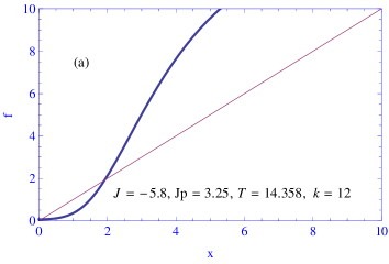
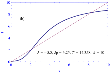
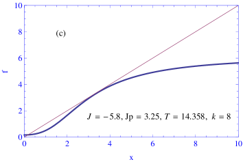
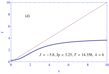
Figure 2. Graphs of the function $f$ defined in (4.28) for $J=-5.8,J_{p}=3.25,T=14.358$ and even integers $k=12,10,8,6$.

In Figure 2 (c), there exists two positive fixed point of the function (4.28) for $J=-5.8,J_{p}=3.25,T=14.358$ and $k=8$.

In Figure 2 (d), we are also able to find that, for the parameters $J=-5.8,J_{p}=3.25,T=14.358$ and $k=6$, the function (4.28) has a unique positive fixed point. Therefore, the phase transition does not occur for $J=-5.8,J_{p}=3.25,T=14.358$ and $k=6$.

We note that for $J=-5.8,J_{p}=3.25,T=14.358$ and $k=10$, the function (4.28) have three positive fixed points as $x_{1}^{*}=0.106457,x_{2}^{*}=2.13383,x_{3}^{*}=8.30085.$ Figure 2 (b) shows that for all $x\in(x_{2}^{*},x_{3}^{*})$, $\lim\limits_{n\rightarrow\infty}f^{n}(x)=x_{3}^{*}.$ Similarly, for all $x\in(x_{1}^{*},x_{2}^{*})$, $\lim\limits_{n\rightarrow\infty}f^{n}(x)=x_{1}^{*}.$ Therefore, the fixed points $x_{1}^{*}$ and $x_{3}^{*}$ are stable and $x_{2}^{*}$ is unstable.

Therefore, there is a critical temperature $T_{c}>0$ such that for $T<T_{c}$ this system of equations has 3 positive solutions: $h_{1}^{*};h_{2}^{*};h_{3}^{*}.$ We denote the Gibbs measure that corresponds to the root $h_{1}^{*}$ (and respectively $h_{2}^{*};h_{3}^{*}$) by $\mu^{(1)}$ (and respectively $\mu^{(2)}$,$\mu^{(3)}$).

Remark 4.4.

We can conclude that the Gibbs measures $\mu_{1}^{*}$ and $\mu_{3}^{*}$ corresponding to the stable fixed points $x_{1}^{*}$ and $x_{3}^{*}$ are extreme Gibbs distributions (for details [20, 28]).

Remark 4.5.

For $J=-5.8,J_{p}=3.25,T=14.358$ and $k>6$ ($k$ is even integer), the model has phase transition. For $J=-5.8,J_{p}=3.25,T=14.358$ and $k=6$, the phase transition of the model does not occur.

5. The Recurrence equations for $k$-odd.

Let us derive the recurrence equations to describe the existence of the translation-invariant Gibbs measures (TIGMs) associated to the model (2.2) on the Cayley tree of order $k$-odd.

From the equations (3.1), (3.2) and (4), one get the following equations:

$$u_{1}^{{}^{\prime}} = \exp(h_{B_{1}(x^{(0)});S_{0}^{k}(+)})=L_{2}\left(\sum_{i=0}^{k}(ab)^{-2i+k}\left(\begin{array}[]{c}k\\ i\end{array}\right)u_{1+i}^{(-1)^{i}}\right)^{k}$$ (5.3)

$$(u_{k+1}^{{}^{\prime}})^{-1} = \exp(-h_{B_{1}(x^{(0)});S_{k}^{0}(+)})={{L}_{2}}{{\left(\sum\limits_{i=0}^{k}{\left(\begin{array}[]{c}k\\ i\end{array}\right){{\left(\frac{b}{a}\right)}^{-2i+k}}}u_{2+i+k}^{{{(-1)}^{1+i}}}\right)}^{k}}.$$ (5.6)

For the configuration $S_{0}^{k}(\sigma({{x}^{(0)}})=-)=\left(\begin{matrix}\overbrace{+,\cdots,+,+}^{k-odd}\\ -\\ \end{matrix}\right)$, similarly to (5.3) and (5.6) we obtain

$${{\left(u_{k+2}^{{}^{\prime}}\right)}^{-1}}=\exp(-{{h}_{{{B}_{1}}({{x}^{(0)}});S_{0}^{k}(-)}})={{L}_{2}}{{\left(\sum\limits_{i=0}^{k}{\left(\begin{array}[]{c}k\\ i\end{array}\right){{\left(\frac{a}{b}\right)}^{-2i+k}}}u_{1+i}^{{{(-1)}^{i}}}\right)}^{k}}.$$ (5.9)

Lastly, for the configuration $S_{k}^{0}(\sigma({{x}^{(0)}})=-)=\left(\begin{matrix}\overbrace{-,\cdots,-,-}^{k-odd}\\ -\\ \end{matrix}\right)$ we have

$$\left(u_{2(k+1)}^{{}^{\prime}}\right)=\exp({{h}_{{{B}_{1}}({{x}^{(0)}});S_{k}^{0}(-)}})={{L}_{2}}{{\left(\sum\limits_{i=0}^{k}{\left(\begin{array}[]{c}k\\ i\end{array}\right){{(ab)}^{2i-k}}}u_{2+i+k}^{{{(-1)}^{1+i}}}\right)}^{k}}.$$ (5.12)

From the equations (5.3)-(5.12), it is obvious that

$$e^{(-1)^{m}h_{B_{1}(x^{(0)});S_{m}^{k-m}(+)}} = \left(e^{h_{B_{1}(x^{(0)});S_{0}^{k}(+)}}\right)^{\frac{k-m}{k}}\left(e^{-h_{B_{1}(x^{(0)});S_{k}^{0}(+)}}\right)^{\frac{m}{k}}$$ (5.13)

$$e^{(-1)^{m+1}h_{B_{1}(x^{(0)});S_{m}^{k-m}(-)}} = \left(e^{-h_{B_{1}(x^{(0)});S_{0}^{k}(-)}}\right)^{\frac{k-m}{k}}\left(e^{h_{B_{1}(x^{(0)});S_{k}^{0}(-)}}\right)^{\frac{m}{k}}.$$ (5.14)

By substituting variables $u_{i}=v_{i}^{k}$ for $i=1,2,\cdots,2(k+1)$ in the recurrent equations (5.3)-(5.12), after small calculations, we can express a new recurrence system in a simpler form:

$$(v^{\prime}_{1}) = \sqrt[k]{L_{2}}\left(\frac{1+(ab)^{2}v_{1}v_{k+1}}{abv_{k+1}}\right)^{k},$$ (5.15)

$$(v^{\prime}_{k+1})^{-1} = \sqrt[k]{L_{2}}\left(\frac{b^{2}+a^{2}v_{k+2}v_{2(k+1)}}{abv_{k+2}}\right)^{k},$$ (5.16)

$$(v^{\prime}_{k+2})^{-1} = \sqrt[k]{L_{2}}\left(\frac{b^{2}+a^{2}v_{1}v_{k+1}}{abv_{k+1}}\right)^{k},$$ (5.17)

$$(v^{\prime}_{2(k+1)}) = \sqrt[k]{L_{2}}\left(\frac{1+(ab)^{2}v_{k+2}v_{2(k+1)}}{abv_{k+2}}\right)^{k}.$$ (5.18)

5.1. The translation-invariant Gibbs measures: Odd case

In this subsection, we will identify the solutions of the system of nonlinear equations (5.15)-(5.18) to describe the translation invariant Gibbs measures associated to the model (2.2) on the arbitrary odd-order Cayley tree.

Remark 5.1.

By using the equations (5.13) and (5.14), it can be shown that if the vector-valued function $\textbf{h}(x)$ given in (4.23) has the following form:

$$\textbf{h}(x)=(p,\cdots,\frac{(-1)^{m}((k-m)p-mq)}{k},\cdots,q,r,\cdots,\frac{(-1)^{m+1}(ms-(k-m)r)}{k},\cdots,s),$$

where $p,q,r,s\in\mathbb{R}$, then the consistency condition (3.5) is satisfied.

Now, we want to find the TIGMs for considered case. To do so, we introduce some notations. Define transformation

$$\textbf{F}=(F_{1},F_{k+1},F_{k+2},F_{2(k+1)}):\mathbf{R}^{4}_{+}\rightarrow\mathbf{R}^{4}_{+}$$ (5.19)

such that

$$v^{\prime}_{1} = F_{1}(v_{1},v_{k+1},v_{k+2},v_{2(k+1)}),$$

$$v^{\prime}_{k+1} = F_{k+1}(v_{1},v_{k+1},v_{k+2},v_{2(k+1)}),$$

$$v^{\prime}_{k+2} = F_{k+2}(v_{1},v_{k+1},v_{k+2},v_{2(k+1)}),$$

$$v^{\prime}_{2(k+1)} = F_{2(k+1)}(v_{1},v_{k+1},v_{k+2},v_{2(k+1)}).$$

The fixed points of the cavity equation $\textbf{v}=\textbf{F}(\textbf{v})$ given in the Eq. (5.19) describe the translation invariant Gibbs measures associated to the model (2.2), where $\textbf{v}=(v_{1},v_{k+1},v_{k+2},v_{2(k+1)})$ and $k$ is any positive odd integer greater than 1.

Divide (5.15) by (5.16), then we have

$$v_{k+1}^{2k+1}v_{k+2}^{-k}=\left(\frac{1+(ab)^{2}v_{k+1}^{k+1}}{b^{2}+a^{2}v_{k+2}^{k+1}}\right)^{k}.$$ (5.20)

Similarly, divide (5.18) by (5.17), then one gets

$$v_{k+2}^{2k+1}v_{k+1}^{-k}=\left(\frac{1+(ab)^{2}v_{k+2}^{k+1}}{b^{2}+a^{2}v_{k+1}^{k+1}}\right)^{k}.$$ (5.21)

Multiply the equations (5.20) and (5.21), we obtain

$$v_{k+1}^{k+1}v_{k+2}^{k+1}=\left(\frac{1+(ab)^{2}v_{k+1}^{k+1}}{b^{2}+a^{2}v_{k+2}^{k+1}}\right)^{k}\left(\frac{1+(ab)^{2}v_{k+2}^{k+1}}{b^{2}+a^{2}v_{k+1}^{k+1}}\right)^{k}.$$

Let us consider set

$$B=\left\{(v_{1},v_{k+1},v_{k+2},v_{2(k+1)})\in\mathbb{R}_{+}^{4}:v_{1}=v_{k+1}^{k}=v_{2({k+1})}=v_{{k+2}}^{k}\right\}.$$ (5.22)

Assume that $v_{k+1}^{k+1}=v_{k+2}^{k+1}=x$, and $a^{2}=c$, $b^{2}=d$ then we get

$$x=\left(\frac{1+cdx}{d+cx}\right)^{k}=:g(x).$$ (5.23)

Remark 5.2.

If $(v_{1},v_{k+1},v_{k+2},v_{2(k+1)})\in B$, that is

$$h_{B_{1}(x);S_{0}^{k}(+)}=kh_{B_{1}(x);S_{k}^{0}(+)}=kh_{B_{1}(x);S_{0}^{k}(-)}=h_{B_{1}(x);S_{k}^{0}(-)}$$

then the equation (5.23) is valid. Also, one can verify that $\textbf{F}(B)\subset B.$ That is, the set $B$ is an invariant set under the mapping F.

Now we examine how many solutions the equation $g(x)=x$ has. Thus, similarly to the Proposition 4.2, we have the following Proposition. Here, by using the procedure given in [26, Proposition 10.7] we will describe the number of fixed points of the function $g$ in (5.23).

Proposition 5.1.

The equation (5.23) (with $x\geq 0,c>0,d>0$) has one solution if $d<1$. If $d>\frac{k+1}{k-1}$ then there exists $\eta_{1}(c,d)$, $\eta_{2}(c,d)$ with $0<\eta_{1}(c,d)<\eta_{2}(c,d)$ such that equation (4.28) has 3 solutions if $\eta_{1}(c,d)<m<\eta_{2}(c,d)$ and has 2 solutions if either $\eta_{1}(c,d)=m$ or $\eta_{2}(c,d)=m$. In fact

$$\eta_{i}(c,d)=\frac{1}{x_{i}}\left(\frac{1+cdx_{i}}{d+cx_{i}}\right)^{k}.$$

where $x_{1},x_{2}$ are the solutions of quadratic equation $c^{2}dx^{2}-c(d^{2}(k-1)-(1+k))x+d=0.$

The proof of Proposition 5.1 can be done easily by following the procedure in Proposition 4.2.

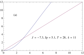
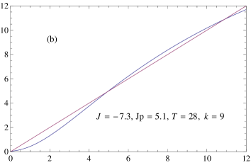
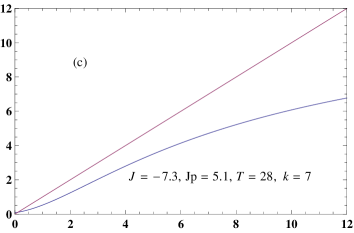
Figure 3. Graphs of the function $g$ given in (4.28) for $J=-7.3,Jp=5.1,T=28$ and odd integers $k=11,9,7$, respectively.

5.2. Illustrative Example: Odd Case

We have manipulated the equation (5.23) via Mathematica [39]. We have obtained at most 3 positive real roots for some parameters $J$ and $J_{p}$ and temperature $T$. As an illustrative example, the Figures 3 (a)-(b) show that there are 3 positive fixed points of the function (5.23) for $J=-7.3,J_{p}=5.1,T=28$ and $k=11,9$ values. Therefore, we have demonstrated the occurrence of phase transitions. The Figures 3 (a)-(b) shows that there are three positive fixed points of the function $g$ for $J=-7.3,J_{p}=5.1,T=28$ and $k=11,9$.

In the Figure 3 (c), there exists a unique positive fixed point of the function (5.23) for $J=-7.3,J_{p}=5.1,T=28$ and $k=7$. Therefore, the phase transition does not occur for $J=-7.3,J_{p}=5.1,T=28$ and $k=7$.

We can explicitly compute the fixed points of the function (5.23) for given some parameters $J,J_{p},T$ and $k$. For example, for $J=-7.3,J_{p}=5.1,T=28$ and $k=9$, the function (5.23) have three positive fixed points as $x_{1}^{*}=0.0448184,x_{2}^{*}=4.93008,x_{3}^{*}=10.8931.$ The Figure 3 (b) shows that for all $x\in(x_{2}^{*},x_{3}^{*})$, $\lim\limits_{n\rightarrow\infty}g^{n}(x)=x_{3}^{*}.$ Similarly, for all $x\in(x_{1}^{*},x_{2}^{*})$, $\lim\limits_{n\rightarrow\infty}g^{n}(x)=x_{1}^{*}.$ Therefore, the fixed points $x_{1}^{*}$ and $x_{3}^{*}$ are stable and $x_{2}^{*}$ is unstable.

Remark 5.3.

As concluded in Remark 4.4, we can see that the Gibbs measures $\mu_{1}^{*}$ and $\mu_{3}^{*}$ corresponding to the stable fixed points $x_{1}^{*}$ and $x_{3}^{*}$ are extreme Gibbs distributions (for details [20, 28]).

Remark 5.4.

There is a critical temperature $T_{c}>0$ such that for $T<T_{c}$ the system of nonlinear equations (5.15)-(5.18) has 3 positive solutions: $h_{1}^{*};h_{2}^{*};h_{3}^{*}.$ We denote the Gibbs measure that corresponds to the root $h_{1}^{*}$ (and respectively $h_{2}^{*};h_{3}^{*}$) by $\mu^{(1)}$ (and respectively $\mu^{(2)}$,$\mu^{(3)}$).

6. Conclusions

In the present paper, we have proposed a rigorous measure-theoretical approach to investigate the Gibbs measures with memory of length 2 associated with the Ising-Vanniminus model on the arbitrary order Cayley tree. We have generalized the results conjectured in [3, 4] for an arbitrary order Cayley tree. We have used the Markov random field method to describe the Gibbs measures. We constructed the recurrence equations corresponding generalized ANNNI model. We have satisfied the Kolmogorov consistency condition. We have explained whether the number of branches of tree does not change the number of Gibbs measures. We have concluded that the order $k$ of the tree significantly affects the occurrence of phase transition. Also, we have seen that the role of $k$ is rather significant on the number of Gibbs measures. Exact description of the solutions of the system of recurrence equations (4.19)-(4.22) (and (5.15)-(5.18)) is rather tricky. Therefore, we were able to resolve only case (4.25) (and (5.22)) for even $k$ (and odd $k$, respectively), the other cases remain open problem. Also, depending on the even and odd of $k$, the recurrence equations obtained for even branch totaly differ from odd branch.

Note that for many problems the solution on a tree is much simpler than on a regular lattice such as $d$-dimensional integer lattice and is equivalent to the standard Bethe-Peierls theory [6]. Although the Cayley tree is not a realistic lattice; however, its amazing topology makes the exact calculations of various quantities possible. Therefore, the results obtained in our paper can inspire to study the Ising and Potts models over multi-dimensional lattices or the grid ${{\mathbb{Z}}^{d}}$. After a glimpse of some applications, we believe now that new theoretical developments can be inspired by concrete problems. By considering the method used in this paper, the investigation of Gibbs measures with memory of length $n>2$ on arbitrary order Cayley tree and Cayley tree-like lattices [41, 42, 43] is planned to be the subject of forthcoming publications.

References

• [1] P. M. Bleher, Extremity of the Disordered Phase in the Ising Model on the Bethe Lattice, Commun. Math. Phys. 128, 411-419 (1990). doi: 10.1007/BF02108787
• [2] N. Ganikhodjaev, S. Uguz, Competing binary and k-tuple interactions on a Cayley tree of arbitrary order, Physica A 390, 4160 4173 (2011). doi: 10.1016/j.physa.2011.06.044
• [3] H. AkΔ±n, Using New Approaches to obtain Gibbs Measures of Vannimenus model on a Cayley tree, Chinese Journal of Physics, 54 (4), 635-649 (2016). doi: 10.1016/j.cjph.2016.07.010
• [4] H. AkΔ±n, Phase transition and Gibbs Measures of Vannimenus model on semi-infinite Cayley tree of order three, International Journal of Modern Physics B, to appear, arXiv:1608.06178 [math.DS]
• [5] M. Denker, C. Grillenberger, and K. Sigmund, Ergodic Theory on Compact Spaces, Lecture Notes in Math. 527, Springer, Berlin, 1976.
• [6] S. Katsura, T. Makoto, Bethe lattice and the Bethe approximation, Prog. Theor. Phys. 51 (1), 82-98 (1974). doi: 10.1143/PTP.51.824
• [7] M. Ostilli, Physica A 391, 3417 3423 (2012). doi: 10.1016/j.physa.2012.01.038
• [8] H.A. Bethe, Statistical theory of superlattices, Proc. Roy. Soc. London Ser A, Mathematical and Physical Sciences 150 (871), 552-575 (1935).
• [9] H.O. Georgii, Gibbs measures and phase transitions (Walter de Gruyter, Berlin, 1988)
• [10] P. M. Bleher, J. Ruiz, and V. A. Zagrebnov, On the purity of the limiting Gibbs state for the Ising model on the Bethe lattice, J. Stat. Phys. 79, 473-482 (1995). doi: 10.1007/BF02179399
• [11] P. M. Bleher and N. N. Ganikhodjaev, On Pure Phases of the Ising Model on the Bethe Lattices, Theory Probab. Appl. 35, 216-227 (1990). doi: 10.1137/1135031
• [12] N. N. Ganikhodjaev, S. Temir, and H. AkΔ±n, Modulated Phase of a Potts Model with Competing Binary Interactions on a Cayley tree, J. Stat. Phys. 137, 701 (2009). doi: 10.1007/s10955-009-9869-z
• [13] H. AkΔ±n, H. SaygΔ±lΔ±, Phase transition of the Potts model with three competing interactions on Cayley tree of order 3, AIP Conference Proceedings 1676, 020026 (2015); http://doi.org/10.1063/1.4930452
• [14] H. AkΔ±n, H. SaygΔ±lΔ±, On Gibbs measures of the Potts model with three competing interactions on Cayley tree of order 3, Acta Physica Polonica A, 129 (4), 845-848 (2016).
doi: 10.12693/APhysPolA.129.845
• [15] N. N. Ganikhodjaev, H. AkΔ±n, and T. Temir, Potts model with two competing binary interactions, Turk. J Math. 31 (3), 229-238 (2007).
• [16] N. N. Ganikhodjaev, S. Temir, and H. Akin, The exact solution of the Potts models with external magnetic field on the Cayley tree, CUBO A Math. Jour. 7 (3), 37-48 (2005).
• [17] S. Uguz, N. N. Ganikhodjaev, H. AkΔ±n, and S. Temir, Lyapunov exponents and modulated phases of an ising model on cayley tree of arbitrary order, Int. J. Mod. Phys. C 23, 1250039 (2012) [15 pages] doi: 10.1142/S0129183112500398
• [18] N. Ganikhodjaev, H. AkΔ±n, S. Temir, S. Uguz, and A. M. Nawi, Strange Attractors in the Vannimenus Model on an Arbitrary Order Cayley Tree, Journal of Physics: Conference Series, 435 (2013) 012031 doi:10.1088/1742-6596/435/1/012031
• [19] S. Inawashiro and C. J. Thompson, , Competing Ising Interactions and Chaotic Glass-Like Behaviour on a Cayley tree, Physics Letters 97A, 245-248 (1983). doi: 10.1016/0375-9601(83)90758-2
• [20] D. Ioffe, A note on the extremality of the disordered state for the Ising model on the Bethe lattice Lett. Math. Phys. 37, 137-143 (1996). doi: 10.1007/978-3-0348-9037-3-1
• [21] J. Vannimenus, Modulated phase of an Ising system with competing interactions on a Cayley tree, Zeitschrift fur Physik B Condensed Matter 43 (2), 141-148 (1981). doi: 10.1007/BF01293605
• [22] H. AkΔ±n, U. A. Rozikov, and S. Temir, A new set of limiting Gibbs measures for the Ising model on a Cayley tree. J. Stat. Phys. 142 (2), 314-321 (2011). doi: 10.1007/s10955-010-0106-6
• [23] R. J. Baxter, Exactly Solved Models in Statistical Mechanics, Academic Press, London/ New York, (1982).
• [24] R. L. Dobrushin, Description of a random field by means of conditional probabilities and conditions of its regularity Theor. Prob. Appl. 13, 197-225 (1968). doi: 10.1137/1113026
• [25] M. Fannes and A. Verbeure, On Solvable Models in Classical Lattice Systems, Commun. Math. Phys. 96, 115-124 (1984). doi: 10.1007/BF01217350
• [26] Ch. J. Preston, Gibbs States on Countable Sets, Cambridge Univ. Press, Cambridge (1974).
• [27] H. AkΔ±n and S. Temir, On phase transitions of the Potts model with three competing interactions on Cayley tree, Condensed Matter Physic 14 (2), 23003:1-11 (2011). doi: 10.5488/CMP.14.23003
• [28] N. N. Ganikhodjaev, H. AkΔ±n, S. Uguz, and T. Temir, On extreme Gibbs measures of the Vannimenus model, J. Stat. Mech. Theor. Exp. 03 (2011): P03025. doi: 10.1088/1742-5468/2011/03/P03025
• [29] N. Ganikhodjaev, Ising model with competing ”uncle-nephew” interactions, Phase Transitions, 89 (12), 1196-1202 (2016). doi: 10.1080/01411594.2016.1156680
• [30] D. Gandolfo, J. Ruiz, and S. Shlosman, A manifold of pure Gibbs states of the Ising model on a Cayley tree, J. Stat. Phys. 148, 999-1005 (2012). doi: 10.1007/s10955-012-0574-y
• [31] S. Zachary, Countable state space Markov random Felds and Markov chains on trees, Ann. Prob. 11, 894-903 (1983).
• [32] N. N. Ganikhodjaev, H. AkΔ±n, S. Uguz, and S. Temir, Phase diagram and extreme Gibbs measures of the Ising model on a Cayley tree in the presence of competing binary and ternary interactions, Phase Transitions 84, no. 11-12, 1045-1063 (2011). doi: 10.1080/01411594.2011.579395
• [33] U. A. Rozikov, H. AkΔ±n, and S. Uguz, Exact Solution of a generalized ANNNI model on a Cayley tree, Math. Phys. Anal. Geom. 17, 103-114 (2014). doi: 10.1007/s11040-014-9144-7
• [34] Ya G. Sinai, Theory of Phase Transitions: Rigorous Results (Pergamon, 1983).
• [35] U. A. Rozikov, Gibbs Measures on Cayley trees, World Scientific Publishing Company (2013).
• [36] D. Gandolfo, M. M. Rakhmatullaev, U. A. Rozikov, and J. Ruiz, On free energies of the Ising model on the Cayley tree, J. Stat. Phys. 150 (6), 1201-1217 (2013). doi: 10.1007/s10955-013-0713-0
• [37] D. Gandolfo, F. H. Haydarov, U. A. Rozikov, and J. Ruiz, New phase transitions of the Ising model on Cayley trees, J. Stat. Phys. 153 (3), 400-411 (2013). doi: 0.1007/s10955-013-0836-3
• [38] F. Mukhamedov, M. Dogan, and H. AkΔ±n, Phase transition for the p-adic Ising-Vannimenus model on the Cayley tree, J. Stat. Mech. Theor. Exp. P10031, pp. 1-21. (2014). doi: 10.1088/1742-5468/2014/10/P10031
• [39] Wolfram Research, Inc., Mathematica, Version 8.0, Champaign, IL (2010).
• [40] H. AkΔ±n, N. N. Ganikhodjaev, S. Uguz, and S. Temir, Periodic extreme Gibbs measures with memory length 2 of Vannimenus model, AIP Conf. Proc. 1389 (1), 2004-2007, (2011). doi: 10.1063/1.3637008.
• [41] S. Uguz and H. AkΔ±n, Modulated Phase of an Ising System with quinary and binary interactions on a Cayley tree-like lattice: Rectangular Chandelier. Chin. J. Phys. 49 (3), 788-801 (2011).
• [42] S. Uguz and H. AkΔ±n, Phase diagrams of competing quadruple and binary interactions on Cayley tree-like lattice: Triangular Chandelier Physica A 389, 1839 1848 (2010). doi:10.1016/j.physa.2009.12.057
• [43] H. Moraal, Ising spin systems on Cayley tree-like lattices: Spontaneous magnetization and correlation functions far from the boundary Physica A 92, 305-314 (1978). doi:10.1016/0378-4371(78)90037-7