Change detection in complex dynamical systems using intrinsic phase and amplitude synchronization

Abstract

We present an approach for the detection of sharp change points (short-lived and persistent) in nonlinear and nonstationary dynamic systems under high levels of noise by tracking the local phase and amplitude synchronization among the components of a univariate time series signal. The signal components are derived via Intrinsic Time scale Decomposition (ITD)–a nonlinear, non-parametric analysis method. We show that the signatures of sharp change points are retained across multiple ITD components with a significantly higher probability as compared to random signal fluctuations. Theoretical results are presented to show that combining the change point information retained across a specific set of ITD components offers the possibility of detecting sharp transitions with high specificity and sensitivity. Subsequently, we introduce a concept of mutual agreement to identify the set of ITD components that are most likely to capture the information about dynamical changes of interest and define an InSync statistic to capture this local information. Extensive numerical, as well as real-world case studies involving benchmark neurophysiological processes and industrial machine sensor data, suggest that the present method can detect sharp change points, on an average 62% earlier (in terms of average run length) as compared to other contemporary methods tested.

I Introduction

CONVENTIONALLY, the detection of anomalies and change points involves testing a hypothesis, $H_{o}:\bm{\theta=\theta_{0}}$ against $H_{a}:\bm{\theta\neq\theta_{0}}$ over some process parameters $\bm{\theta}$. This implicitly assumes that the process exhibits stationarity. In contrast, real-world processes are inherently nonstationary, i.e., they are continuously changing such as modulations to autocorrelation structure [choi2008sequential] or are piece-wise stationary [wang2018dirichlet]. Examples of nonstationary processes include seismic waves (see Fig. 1(a)), speech signals such as the word “greasy” as shown in Fig. 1(b), etc. While nonstationary processes are time varying, abrupt changes may occur in the structure [choi2008sequential] or the distributional characteristics [wang2018dirichlet] of the underlying processes. For instance, change in the autocorrelation of a slowly varying first order auto-regressive (AR) process as shown in Fig. 1(c).

Critical anomalies may occur when real-world processes transition sharply from one dynamic behavior to the other [basseville1993detection, nikiforov1999quadratic]. These anomalies can either be persistent [wang2014change] (e.g., changes in the covariance structure) or short-lived [barry1993bayesian] that typically do not last beyond the sampling interval of the time series, as in singularities (or spikes). Timely detection of these sharp transitions to an anomalous behavior is crucial for effective process control. However, the existing change detection models are severely limited in discerning these sharp transitions [nemeth2014sequential]. Much of the existing change detection methods are based on utilizing the amplitude information [gao2000structures]; only a handful of the methods have investigated the instantaneous phase properties of the underlying time series signal [chiang2000phase].

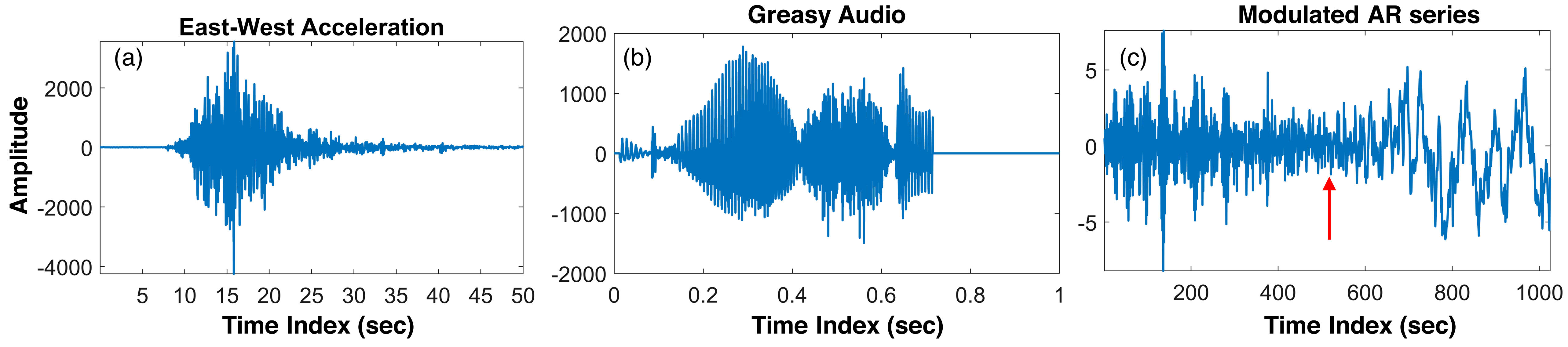
Figure 1: (a) Loma-Prieta Earthquake data (b) “greasy” audio signal (c) modulated autoregressive time series with abrupt change at $t=512$ pointed by the arrow.

The importance of phase is becoming increasingly evident in various domains, such as image analysis and reconstruction [oppenheim1981importance], electrophysiology [varela2001brainweb], etc. Phase-based change detection methods have been shown to detect some of the critical events that might go undetected if we rely only on the amplitude information. In many instances, the signal phases exhibited a higher level of synchronization during such events as compared to the amplitudes [rosenblum1996phase]. However, the current phase synchronization approaches require multiple signals (or channels) to utilize the phase information. In the absence of such multi-dimensional time series signals, we propose to decompose the univariate time series signal $x(t)\in\mathbb{R},t\in\mathbb{Z}^{+}$ into multiple components to extract the phase information.

Unlike stationary Gaussian time series signals, decomposition of nonlinear and nonstationary signals is a non-trivial task [frei2007intrinsic]. Parametric signal decomposition methods such as short-time Fourier, Wavelet or Wigner-Ville transform [Cohen1995] tend to be sub-optimal since they assume an a priori basis and often yield poor or inaccurate time-frequency localization. This is a critical issue, especially when detecting short-lived change points. Alternatively, non-parametric methods, e.g., Empirical Mode Decomposition [huang903empirical] or Independent Component Analysis [oja2000independent] offer a data-driven approach with intrinsic basis functions for the decomposition of nonstationary signals. However, these methods cannot be used for real-time applications with streaming data because the decomposition is not causal, i.e., the basis functions are sensitive to the signal length and may change as more data is collected. Such decomposition methods are often employed for off-line detection of change points, where the complete time series is available, and the emphasis is on the accuracy of the detection. However, they may not be pertinent for online change point detection, where the objective is to detect the change point as quickly as possible while satisfying the constraints on the false alarms. Frie and Osorio’s Intrinsic Time Scale Decomposition (ITD) overcomes many of these limitations [frei2007intrinsic]. The elementary decomposition step in ITD considers the signal segment only between consecutive extrema. This allows for a real-time signal decomposition approach with temporal localization of signal features, e.g., change points, across multiple decomposition levels.

In this paper, we present an approach to detect sharp changes (short-lived and persistent) in noisy real-world processes based on combining the phase and amplitude synchronization among multiple levels of ITD components. The specific contributions of this paper are:

1. We derive theoretical results to show that sharp change point features are retained across two or more ITD components with probability more than $0.95$. In contrast, this probability is less than $0.05$ for random signal features. This increases the sensitivity and specificity for detecting change points.

2. We introduce a concept of mutual agreement to identify a set of ITD components that are likely to retain the change point information. Subsequently, we develop a change detection statistic called InSync that fuses the phase and amplitude information from ITD components identified via mutual agreement.

3. We perform extensive numerical and real-world case studies involving short-lived and persistent changes under various process conditions to establish the performance of the present method. We also present the significance level and the rejection criteria (specified in terms of average run length (ARL)) for detecting changes based on the InSync statistic.

We compare the performance of our method with those of conventional approaches, mainly Exponentially Weighted Moving Average (EWMA) and rather contemporary methods including, Wavelet based CUSUM (WCUSUM) method that employs wavelets coefficients to determine the optimal monitoring levels [guo2012multiscale] and Dirichlet Process Gaussian State Machine (DPGSM) [wang2018dirichlet] where a time series is modeled as a mixture of Gaussian and changes occur when the process transitions from one state to the other. We also compare our results with two benchmark change detection packages, CPM [ross2015parametric] and changepoint [killick2014changepoint], each of which contains the implementation of several state-of-the-art change detection approaches. We also compare the computational complexity of these algorithms in the context of online change detection.

The remainder of this paper is organized as follows: in Section 2, we present the ITD algorithm and discuss its relevant properties. In Section 3, we introduce the concepts of intrinsic phase synchronization and mutual agreement followed by the InSync statistic. Section 4 presents the case studies and comparative results followed by concluding remarks and a brief discussion on the performance and limitations of the proposed method in Section 5.

II Overview and properties of ITD

As noted in the preceding section, we utilize ITD to decompose a signal into different components and use phase and amplitude synchronization among a specific set of ITD components to develop a change detection statistic. In this section, we begin with a brief overview of ITD and analyze the behavior of ITD components at sharp change points.

II-A Intrinsic Time Scale Decomposition

ITD belongs to a general class of Volterra series expansions [Franz:2011] that iteratively extracts the baseline component of a nonlinear or nonstationary signal $x(t)$ such that the residual is a proper rotation, i.e., the successive extrema lies on the opposite side of the zero line [frei2007intrinsic]. Formally, $x(t)$ is decomposed as:

$$x(t)=\mathcal{L}(x(t))+R(t)$$

Here, $\mathcal{L}(\cdot)$ is the baseline extracting operator such that $\mathcal{L}(x(t))=L(t)$ is the baseline component and $R(t)$ is the residual, referred to as the rotation component.

Let us denote the local extrema of $x(t)$ by $\tau_{k},k=1,2,\ldots,N$ where $N$ is the total number of local extrema observed in $x(t)$. For simplicity, let $x_{k}$ and $L_{k}$ denote $x(\tau_{k})$ and $L(\tau_{k})$. Then the baseline extracting operator is defined piecewise on the interval $t\in[\tau_{k},\tau_{k+1}]$ between successive extrema as:

$$\mathcal{L}(x(t))\triangleq L(t)=L_{k}+\left(\frac{L_{k+1}-L_{k}}{x_{k+1}-x_{k}}\right)(x(t)-x_{k})$$ (1)

where

$$L_{k+1}=\frac{1}{2}\left[x_{k}+\left(\frac{\tau_{k+1}-\tau_{k}}{\tau_{k+2}-\tau_{k}}\right)(x_{k+2}-x_{k})\right]+\frac{1}{2}x_{k+1}$$ (2)

Once the input signal $x(t)$ is decomposed into the baseline component and the rotation component, we iterate the decomposition process until a monotonic baseline component is obtained, i.e.,

$$x(t) = \mathcal{L}(x(t))+R(t)$$

$$= \mathcal{L}(\mathcal{L}(x(t))+R(t))+R(t)$$

$$\ldots$$

$$= \sum_{j=1}^{J-1}\mathcal{L}^{j}(R(t))+\mathcal{L}^{J}(x(t))$$

where $\mathcal{L}^{J}(x(t))$ is the monotonic baseline component obtained after the stopping criteria is reached [frei2007intrinsic] and $\mathcal{L}^{j}(R(t))$ is the rotation component at level $j=1,2,...,J-1$. For simplicity, we denote $\mathcal{L}^{j}(R(t))$ as $R^{j}(t)$ and $\mathcal{L}^{j}(x(t))$ as $L^{j}(t)$ such that:

$$x(t)=\sum_{j=1}^{J-1}R^{j}(t)+L^{J}(t)$$ (3)

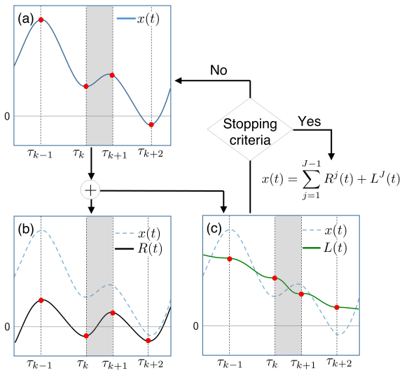
Figure 2: Flow chart showing the recursive decomposition of (a) signal $x(t)$ into (b) a rotation component $R(t)$ and (c) a baseline component $L(t)$. The highlighted region shows the support of the intrinsic basis function defined between two consecutive extrema, $\tau_{k}$ and $\tau_{k+1}$.

In essence, $R^{j}(t)$ captures the “details” of the signal $x(t)$ at the level $j$. The higher the $j$ is, the coarser the details are. As extrema locations are different across different levels, we denote the local extrema at any level $j$ by $\tau^{j}_{k},~{}k=1,2,\ldots,N^{j}$, where $N^{j}$ is the total number of extrema at level $j$. From an algorithm standpoint, the rotation components are obtained recursively by taking the difference between baseline components obtained at two consecutive levels, i.e.,

$$R^{j}(t)=L^{j-1}(t)-L^{j}(t),~{}j=1,2,\ldots,J-1$$ (4)

An instance of the decomposition is shown in Fig. 2. To initialize the decomposition in the interval $[0,\tau_{1}]$, we consider the first point of the signal as an extremum (i.e., $\tau_{0}=0$) and define $L_{0}=(x(\tau_{0})+x(\tau_{1}))/2$.

Since ITD performs the decomposition iteratively between consecutive extrema, the basis functions have finite support (see Fig. 2(c)) which allows for (a) causal representation and (b) temporal localization of the nonlinear and nonstationary signal features across multiple decomposition levels—essential for detecting sharp changes. Also, from Eq. (1), we see that the decomposition involves linear operations which can be performed in $\mathcal{O}(cN)$ time, where $N$ is the number of extrema in $x(t)$ and $c>0$.

II-B Properties of ITD

In this subsection, we extend a simple, yet powerful construct introduced in [restrepo2014defining] to show that the signatures of sharp change points (short-lived as well as persistent) in a given signal are retained across multiple decomposition levels with a specific and significantly higher probability as compared to other random signal features. But first, we present some important properties that will be useful in the representation and understanding of the dynamics of ITD. We begin with a “half-wave” representation of the rotation components as introduced in [frei2007intrinsic]. This representation allows for the definition and extraction of instantaneous phase $\phi_{k}^{j}(t)$ and amplitude $a_{k}^{j}$ over finite support. Figure 3 shows a representative halfwave defined between the zero crossings $(z_{k}^{j},z^{j}_{k+1}]$.

Property 1.

Rotation components can be represented as a concatenation of halfwaves $\hslash^{j}_{k}(t)$ each of which is defined between two consecutive zero crossings $(z_{k}^{j},z^{j}_{k+1}]$, for all $k=1,2,\ldots,N^{j}-1$, i.e.,

$$\hslash^{j}_{k}(t)\triangleq\{R^{j}(t)|t\in(z_{k}^{j},z_{k+1}^{j}]\}$$ (5)

Here, each of the halfwaves $\hslash^{j}_{k}(t)$ has a characteristic amplitude $a^{j}_{k}$ and an instantaneous phase component $\phi^{j}_{k}(t)$. Note that the halfwaves need not be harmonic or even symmetric (i.e., they can be skewed).

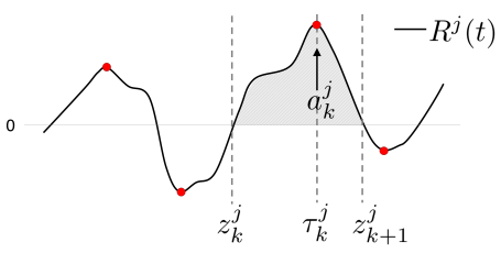
Figure 3: A halfwave, $\hslash^{j}_{k}(t)$ defined on $(z_{k}^{j},z_{k+1}^{j}]$ in $R^{j}(t)$ such that $\tau^{j}_{k}$ is the characteristic extrema of $\hslash^{j}_{k}(t)$.

Property 2.

The value and the location of extrema in the baseline component at $j+1$, i.e., $\{L(\tau^{j+1}_{k}),\tau^{j+1}_{k}\}$ depends only on $\{L(\tau^{j}_{k}),\tau^{j}_{k}\}$ and not on the signal values elsewhere [restrepo2014defining].

Property 2 suggests that in order to obtain $\{L(\tau^{j+1}_{k}),\tau^{j+1}_{k}\}$, we do not need to know the entire baseline component $L^{j}(t)$ but only the value and the location of extrema points in level $j$, i.e., $\{L(\tau^{j}_{k}),\tau^{j}_{k}\}$. In other words, for the purpose of ITD, we can neglect the intermediate points between two successive extrema. We now employ these properties of ITD to determine the probability with which different change point features in $x(t)$ are retained across the levels of ITD.

We first show that a randomly selected point in the in-control region of $x(t)$ is unlikely to be retained across two or more levels of ITD. Following Property 2, we neglect the intermediate points between the successive extrema of $x(t)$ and consider a time series $x_{k}$ whose successive samples are the alternating extrema of $x(t)$ (i.e., maximum followed by a minimum). Such an alternating extrema series is a long-term memory process—its autocorrelation function decays slowly regardless of the distribution (or the autocorrelation function) of $x(t)$. Therefore, without loss of generality (also see [restrepo2014defining]), we define:

$$x_{k}\triangleq(-1)^{k}|w_{k}|;w_{k}\sim\mathcal{N}(0,\sigma^{2}),k\in\mathbb{Z}^{+}$$ (6)

where the magnitudes of successive samples (alternating extrema) are drawn from a white noise process with mean 0 and standard deviation $\sigma$. It turns out that the probability that an extremum at $k$ in level $j$ is retained as an extremum across the subsequent $j+\eta,\eta\in\mathbb{Z}^{+}$ levels decays at a geometric rate as the value of $\eta$ increases. This is presented in the following corollary.

Corollary 1.

The probability that an extremum in the rotation component at level $j$ of $x_{k}$ is retained as an extremum across the subsequent $\eta$ rotation components is approximately equal to $0.24^{\eta}$.

The result follows from [restrepo2014defining]. Please refer to Appendix A of the supplementary material for the proof.

Remark 1.

Corollary 1 shows that the probability with which an extremum in $x_{k}$ is retained across two or more levels of ITD is less than $0.05$. From a change detection standpoint, it is highly desirable to have a low probability for the extrema points in the in-control region to be retained across multiple levels of ITD. This will enhance the specificity when detecting changes based on combining the information across multiple levels.

We now extend this result to a more general scenario by introducing a sharp change in $x_{k}$ such that the baseline component at some level $j$ is represented as:

$$L^{j}_{k}=x_{k}+\text{sgn}(x_{k})\nu\sigma\delta_{k^{*}}$$ (7)

where $\nu$ is a non-negative scale variable, $\delta_{k^{*}}$ is Kronecker delta and $\text{sgn}(\cdot)$ is the sign function. Here, $\nu\delta_{k^{*}}$ is representative of a sharp change point at $k^{*}$. We now determine the probability $P_{e}(\nu)$ that an extremum at $k^{*}$ in level $j$ is retained as an extremum in level $j+1$. For notational simplicity, let $r^{j}_{k}$ and $l^{j}_{k}$ denote $R^{j}(\tau^{j}_{k})$ and $L^{j}(\tau^{j}_{k})$. We now write the probability $P_{e}(\nu)$ as follows:

$$P_{e}(\nu)=P\left(r^{j+1}_{k^{*}}-r^{j+1}_{k^{*}-1}>0\right)P\left(r^{j+1}_{k^{*}}-r^{j+1}_{k^{*}+1}>0\right)$$ (8)

In the following, we show that as $\nu$ increases, there is a dramatic increase in the value of $P_{e}(\nu)$. For this, we first determine the distribution function of $r_{k}^{j+1}$.

Proposition 1.

Let $r^{j+1}_{k}$ be the extremum in the rotation component $R^{j+1}(k)$. The distribution function of the magnitude of $r^{j+1}_{k}$ is given by the convolution of three independent random variables $K_{1},K_{2}$, and $\Gamma$ such that:

$$F_{r^{j+1}_{k}}(r)=\hskip-20.00003pt\underset{\begin{subarray}{c}\{(\kappa_{1},\kappa_{2},\gamma)\in\mathbb{R}^{2}\times[0,2\nu\sigma];\\ \kappa_{1}+\kappa_{2}+\gamma\leq r\}\end{subarray}}{\int\int\int}\hskip-20.00003ptF_{K_{1}}(d\kappa_{1})F_{K_{2}}(d{\kappa_{2}})F_{\Gamma}(d\gamma)$$ (9)

where $K_{i},i=1,2$ are identically distributed random variables that are a sum of independently distributed normal random variables $l^{j}_{k}\sim\mathcal{N}(0,\sigma^{2})$ (see Eqs. (6) and (7)) and $\Theta$, i.e., $K_{i}=l^{j}_{k}+\Theta$ with distribution function given as:

$$F_{K}(l,\theta)=\hskip-20.00003pt\underset{\{(l,\theta)\in\mathbb{R}^{2}:l+\theta\leq\kappa\}}{\int\int}\hskip-20.00003ptG_{\Theta}(d\theta)G_{l^{j}_{k}}(dl)$$

where the distribution function of $\Theta$ is given as:

$$G_{\Theta}(\theta)=\int_{-\infty}^{\theta}\left(\int_{-\infty}^{\infty}f_{U,l^{j}_{k}}\left(l,\frac{\omega}{l}\frac{1}{|l|}dl\right)d\omega\right)$$

with $U\sim\text{Uniform}(0,2)$ and $l^{j}_{k}\sim\mathcal{N}(0,\sigma^{2})$. $\Gamma$ follows a mixture distribution such that:

$$F_{\Gamma}(\gamma)=\int_{0}^{\gamma}\frac{1}{2\nu\sigma}d\omega\bm{1}_{k={k^{*}}\pm 1}+c\bm{1}_{k=k^{*}}$$

where $c>0$ and $\bm{1}_{A}$ is the indicator function for some set $A$.

Please see Appendix B of the supplementary material for the proof of Proposition 1. In the absence of a closed form representation of Eq. (9), we present the following approximation result to simplify the subsequent analysis:

Corollary 2.

Using Gaussian approximation to the distribution function of $r^{j+1}_{k}$, $P_{e}(\nu)$ can be deduced in closed form as:

$$\hat{P}_{e}(\nu)=\left[1-P\left(\mathcal{Z}\leq-\frac{\nu}{\sqrt{2}}\right)\right]^{2}$$ (10)

where $\mathcal{Z}\sim\mathcal{N}(0,1)$.

Proof of the corollary is presented in Appendix C of the supplementary material.

We now use Eq. (10) to determine the probability with which the extremum at $k^{*}$ in level $j$ is retained as an extremum in level $j+1$. The probability as a function of $\nu$ is shown in Fig. LABEL:fig:im4(a) in the black line, labeled as “Approximation”. First, we note that for $\nu=0$, $P_{e}(\nu)\approx 0.25$ is simply is the probability that an extremum in level $j$ is retained as an extremum in level $j+1$ for a white noise signal. This is consistent with the result stated in Corollary 1. Additionally, we note that as $\nu$ increases, there is a sharp increase in the value of $P_{e}(\nu)$, indicating that the information pertaining to a change point is retained across multiple decomposition levels.

To validate the values of $\hat{P_{e}}(\nu)$ obtained by using the Gaussian approximation, we compare with the corresponding probabilities computed numerically by using the analytical form of the distribution function of $r^{j+1}_{k}$ as given in Eq. (9) as well as the empirical estimate of $P_{e}(\nu)$ obtained by using Monte Carlo (MC) simulation. In the MC simulation we perform ITD of $L^{j}_{k}$ with different realizations of $x_{k}$ as given in Eq. (7) and observe the cases when the extremum at $k^{*}$ is retained as an extremum in the subsequent level. To get a consistent estimate of the probability, we performed 100 MC simulations. From Fig. LABEL:fig:im4(a) we notice that the Gaussian approximation $\hat{P_{e}}(\nu)$ closely follows the trend of the probability estimated analytically (blue) as well as via MC simulation (red).

The sharp rise in $P_{e}(\nu)$ as observed in Fig. LABEL:fig:im4(a) can be explained by the Gaussian approximation of $r^{j+1}_{k}$. First, for $r^{j}_{k^{*}}$ to remain an extremum in level $j+1$, we need $r^{j+1}_{k^{*}}-r^{j+1}_{k^{*}\pm 1}>0$. From the proof of Corollary 2 (Appendix C of the supplementary material), we notice that:

$$\left(\hat{r}^{j+1}_{k^{*}}-\hat{r}^{j+1}_{k^{*}\pm 1}\right)\sim\mathcal{N}\left(\frac{\nu}{4},\frac{1}{8}\right)$$

Since the mean of $\hat{r}^{j+1}_{k^{*}}-\hat{r}^{j+1}_{k^{*}\pm 1}$ is a function of $\nu$, the distribution function of $r^{j+1}_{k^{*}}-r^{j+1}_{k^{*}\pm 1}>0$ shifts on the positive $\nu$ axis as the value of $\nu$ increases. As a result, $P_{e}(\nu)$ increases steeply.