Akid: A Library for Neural Network Research and Production From A Dataism Approach

Abstract

Neural networks are a revolutionary but immature technique that is fast evolving and heavily relies on data. To benefit from the newest development and newly available data, we want the gap between research and production as small as possibly. On the other hand, differing from traditional machine learning models, neural network is not just yet another statistic model, but a model for the natural processing engine — the brain. In this work, we describe a neural network library named akid. It provides higher level of abstraction for entities (abstracted as blocks) in nature upon the abstraction done on signals (abstracted as tensors) by Tensorflow, characterizing the dataism observation that all entities in nature processes input and emit out in some ways. It includes a full stack of software that provides abstraction to let researchers focus on research instead of implementation, while at the same time the developed program can also be put into production seamlessly in a distributed environment, and be production ready. At the top application stack, it provides out-of-box tools for neural network applications. Lower down, akid provides a programming paradigm that lets user easily build customized models. The distributed computing stack handles the concurrency and communication, thus letting models be trained or deployed to a single GPU, multiple GPUs, or a distributed environment without affecting how a model is specified in the programming paradigm stack. Lastly, the distributed deployment stack handles how the distributed computing is deployed, thus decoupling the research prototype environment with the actual production environment, and is able to dynamically allocate computing resources, so development (Devs) and operations (Ops) could be separated. It has been open source, and please refer to http://akid.readthedocs.io/en/latest/ for documentation.

1 Introduction

Neural network, which is a cornerstone technique of a pool of techniques under the name of Deep Learning nowadays, seems to have the potential to lead to another technology revolution. It has incurred wide enthusiasm in industry, and serious consideration in public sector and impact evaluation in government. However, though being a remarkable breakthrough in high dimensional perception problems academically and intellectually stimulating and promising [8] [13] [5] [9] [14], it is still rather an immature technique that is fast moving and in short of understanding [11]. Temporarily its true value lies in the capability to solve perception related data analytic problems in industry, e.g. self-driving cars, detection of lung cancer etc. On the other hand, Neural Network is a technique that heavily relies on a large volume of data. It is critical for businesses that use such a technique to leverage on newly available data as soon as possible, which helps form a positive feedback loop that reinforces the quality of service.

Accordingly, to benefit from the newest development and newly available data, we want the gap between research and production as small as possible. In this package, we explore technology stack abstraction that enable fast research prototyping and are production ready.

akid tries to provide a full stack of software that provides abstraction to let researchers focus on research instead of implementation, while at the same time the developed program can also be put into production seamlessly in a distributed environment, and be production ready.

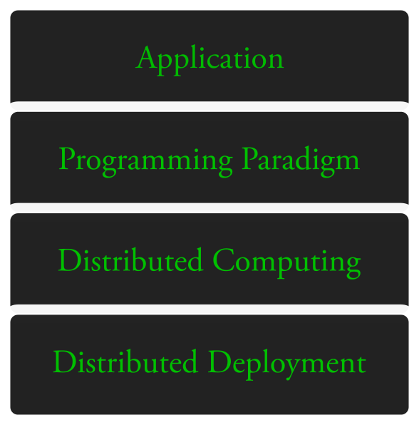
Figure 1: Illustration of stack abstraction of akid.

At the top application stack, it provides out-of-box tools for neural network applications. Lower down, akid provides programming paradigm that lets users easily build customized models, which is the major intellectual innovation of akid that provides higher level of abstraction for entities in nature (abstracted as blocks) upon the abstraction done on signals (abstracted as tensors) by Tensorflow. The distributed computing stack handles the concurrency and communication, thus letting models be trained or deployed to a single GPU, multiple GPUs, or a distributed environment without affecting how a model is specified in the programming paradigm stack. Lastly, the distributed deployment stack handles how the distributed computing is deployed, thus decoupling the research prototype environment with the actual production environment, and is able to dynamically allocate computing resources, so development (Devs) and operations (Ops) could be separated. An illustration of the four stack is shown in Figure 1.

From a feature point of view as a library, it aims to enable fast prototyping and production ready at the same time by offering the following features:

• supports fast prototyping

  • built-in data pipeline framework that standardizes data preparation and data augmentation.

  • arbitrary connectivity schemes (including multi-input and multi-output training), and easy retrieval of parameters and data in the network

  • meta-syntax to generate neural network structure before training

  • support for visualization of computation graph, weight filters, feature maps, and training dynamics statistics.

• be production ready

  • built-in support for distributed computing

  • compatibility to orchestrate with distributed file systems, docker containers, and distributed operating systems such as Kubernetes.

The name comes from the Kid saved by Neo in Matrix, and the metaphor to build a learning agent, which we call kid in human culture.

The rest of the paper discusses related works in Section 2, each stack of akid in detail in Section 3.

2 Related works

akid differs from existing packages from the perspective that it does not aim to be yet another wrapper for another machine learning model. Subtle it seems. The fundamental difference lies in the design. It aims to reproduce how signal propagates in nature by introducing Block. If Tensor in Tensorflow can be viewed as the abstraction for signals in nature, Block can be viewed as the abstraction for entities in nature, which all process inputs in some way, and emit output. It also aims to integrate technology stacks to solve both research prototyping and industrial production by clearly defining the behavior for each stack. We compare akid with existing packages in the following briefly. Note that since Tensorflow is used as the computation backend, we do not discuss speed here, which is not our concern for akid.

Theano [12], Torch [3], Caffe [7], MXNet [2] are packages that aim to provide a friendly front end to complex computation back-end that are written in C++. Theano is a python front end to a computational graph compiler, which has been largely superseded by Tensorflow in the compilation speed, flexibility, portability etc, while akid is built on of Tensorflow. MXNet is a competitive competitor to Tensorflow. Torch is similar with theano, but with the front-end language to be Lua, the choice of which is mostly motivated from the fact that it is much easier to interface with C using Lua than Python. It has been widely used before deep learning has reached wide popularity, but is mostly a quick solution to do research in neural networks when the integration with community and general purpose production programming are not pressing. Caffe is written in C++, whose friendly front-end, aka the text network configuration file, loses its affinity when the model goes more than dozens of layer.

DeepLearning4J is an industrial solution to neural networks written in Java and Scala, and is too heavy weight for research prototyping.

Perhaps the most similar package existing with akid is Keras, which both aim to provide a more intuitive interface to relatively low-level library, i.e. Tensorflow. akid is different from Keras in at least two fundamental aspects. First, akid mimics how signals propagate in nature by abstracting everything as a semantic block, which holds many states, thus is able to provide a wide range of functionalities in a easily customizable way, while Keras uses a functional API that directly manipulates tensors, which is a lower level of abstraction, e.g. it has to do class attributes traverse to retrieve layer weights with a fixed variable name while in akid variable are retrieved by names. Second, Keras mostly only provides an abstraction to build a neural network topology, which is roughly the programming paradigm stack of akid, while akid provides unified abstraction that includes application stack, programming stack, and distributed computing stack. A noticeable improvement is that Keras needs the user to handle communication and concurrency, while the distributed computing stack of akid hides them.

3 akid stack

Now we go technical to discuss each stack provided by akid. The major novel intellectual design of akid is the programming paradigm that provides a higher level abstraction upon signal/tensor. We introduce it first, then we discuss the application stack, and distributed computing and deployment stack.

3.1 Programming Paradigm

3.1.1 It is all about signal processing blocks

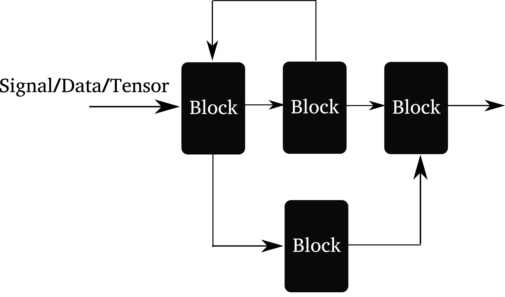
Figure 2: Illustration of the arbitrary connectivity supported by akid. Forward connection, branching and mergine, and feedback connection are supported.

akid builds another layer of abstraction on top of Tensor: Block. Tensor can be taken as the media/formalism signal propagates in digital world, while Block is the data processing entity that processes inputs and emits outputs.

It coincides with a branch of “ideology” called dataism that takes everything in this world is a data processing entity. An interesting one that may come from A Brief History of Tomorrow by Yuval Noah Harari.

Best designs mimic nature. akid tries to reproduce how signals in nature propagates. Information flow can be abstracted as data propagating through inter-connected blocks, each of which processes inputs and emits outputs. For example, a vision classification system is a block that takes image inputs and gives classification results. Everything is a Block in akid.

A block could be as simple as a convonlutional neural network layer that merely does convolution on the input data and outputs the results; it also be as complex as an acyclic graph that inter-connects blocks to build a neural network, or sequentially linked block system that does data augmentation.

Compared with pure symbol computation approach, like the one in tensorflow, a block is able to contain states associated with this processing unit. Signals are passed between blocks in form of tensors or list of tensors. Many heavy lifting has been done in the block (Block and its sub-classes), e.g. pre-condition setup, name scope maintenance, copy functionality for validation and copy functionality for distributed replicas, setting up and gathering visualization summaries, centralization of variable allocation, attaching debugging ops now and then etc.

akid offers various kinds of blocks that are able to connect to other blocks in an arbitrary way, as illustrated in Figure 2. It is also easy to build one’s own blocks. The Kid class is essentially an assembler that assemblies blocks provided by akid to mainly fulfill the task to train neural networks. Here we show how to build an arbitrary acyclic graph of blocks using class Brain, to illustrate how to use blocks in akid.

A brain is the data processing engine to process data supplied by Sensor to fulfill certain tasks. More specifically,

• it builds up blocks to form an arbitrary network

• offers sub-graphs for inference, loss, evaluation, summaries

• provides access to all data and parameters within

To use a brain, data as a list should be fed in, as how it is done in with any other block. Some pre-specified brains are available under akid.models.brains. An example could be:

⬇

# … first get a feed sensor

sensor.setup()

brain = OneLayerBrain(name="brain")

input = [sensor.data(), sensor.labels()]

brain.setup(input)

Note in this case, data() and labels() of sensor returns tensors. It is not always the case. If it does not, saying return a list of tensors, you need do things like:

⬇

input = [sensor.data()]

input.extend(sensor.labels())

Act accordingly.

Similarly, all blocks work this way.

A brain provides easy ways to connect blocks. For example, a one layer brain can be built through the following:

⬇

class OneLayerBrain(Brain):

def __init__(self, **kwargs):

super(OneLayerBrain, self).__init__(**kwargs)

self.attach(

ConvolutionLayer(ksize=[5, 5],

strides=[1, 1, 1, 1],

padding="SAME",

out_channel_num=32,

name="conv1")

)

self.attach(ReLULayer(name="relu1"))

self.attach(

PoolingLayer(ksize=[1, 5, 5, 1],

strides=[1, 5, 5, 1],

padding="SAME",

name="pool1")

)

\parself.attach(InnerProductLayer(

out_channel_num=10, name="ip1"))

self.attach(SoftmaxWithLossLayer(

class_num=10,

inputs=[

{"name": "ip1", "idxs": [0]},

{"name": "system_in", "idxs": [1]}],

name="loss"))

It assembles a convolution layer, a ReLU Layer, a pooling layer, an inner product layer and a loss layer. To attach a block (layer) that directly takes the outputs of the previous attached layer as inputs, just directly attach the block. If inputs exists, the brain will fetch corresponding tensors by name of the block attached and indices of the outputs of that layer. See the loss layer above for an example. Note that even though there are multiple inputs for the brain, the first attached layer of the brain will take the first of these input by default, given the convention that the first tensor is the data, and the remaining tensors are normally labels, which is not used till very late.

As an example to build more complex connectivity scheme, residual units can be built using Brain as shown in Figure 3.

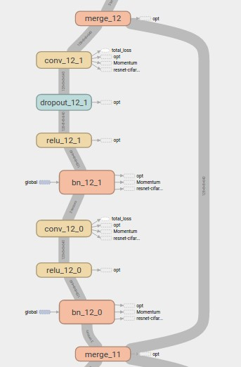
Figure 3: A residual unit. On the left is the branch that builds up patterns complexity, and on the right is the stem branch that shortcuts any layers to any layers. They merge at the at the start and at the end of the branching points.

3.1.2 Self-modifying brains — parameter tuning

akid offers automatic parameter tuning through defining template using tune function. A function tune that takes a Brain jinja2 template class and a parameters to fill the template in runtime.

The tune function would use all available GPUs to train networks with all given different set of parameters. If available GPUs are not enough, the ones that cannot be trained will wait till some others finish, and get its turn.

Tunable parameters are divided into two sets, network hyper parameters, net_paras_list, and optimization hyper parameters, opt_paras_list. Each set is specified by a list whose item is a dictionary that holds the actual value of whatever hyper parameters defined as jinja2 templates. Each item in the list corresponds to a tentative training instance. Network paras and optimization paras combine with each other exponentially (or in Cartesian Product way if we could use Math terminology), which is to say if you have two items in network parameter list, and two in optimization parameters, the total number of training instances will be four.

Given the available GPU numbers, a semaphore is created to control access to GPUs. A lock is created to control access to the mask to indicator which GPU is available. After a process has modified the gpu mask, it releases the lock immediately, so other process could access it. But the semaphore is still not release, since it is used to control access to the actual GPU. A training instance will be launched in a subshell using the GPU acquired. The semaphore is only released after the training has finished.

For example, to tune the activation function and learning rates of a network, first we set up network parameters in net_paras_list, optimization parameters in opt_paras_list, build a network in the setup function, then pass all of it to tune:

⬇

net_paras_list = []

net_paras_list.append({

"activation": [

{"type": "relu"},

{"type": "relu"},

{"type": "relu"},

{"type": "relu"}],

"bn": True})

net_paras_list.append({

"activation": [

{"type": "maxout", "group_size": 2},

{"type": "maxout", "group_size": 2},

{"type": "maxout", "group_size": 2},

{"type": "maxout", "group_size": 5}],

"bn": True})

\paropt_paras_list = []

opt_paras_list.append({"lr": 0.025})

opt_paras_list.append({"lr": 0.05})

\pardef setup(graph):

\parbrain.attach(cnn_block(

ksize=[8, 8],

init_para={

"name": "uniform",

"range": 0.005},

wd={"type": "l2", "scale": 0.0005},

out_channel_num=384,

pool_size=[4, 4],

pool_stride=[2, 2],

activation={{ net_paras["activation"][1] }},

keep_prob=0.5,

bn={{ net_paras["bn"] }}))

\partune(setup, opt_paras_list, net_paras_list)

3.2 Application stack

At the top of the stack, akid could be used as a part of application without knowing the underlying mechanism of neural networks.

akid provides full machinery from preparing data, augmenting data, specifying computation graph (neural network architecture), choosing optimization algorithms, specifying parallel training scheme (data parallelism etc), logging and visualization.

3.2.1 Neural network training — A holistic example

To create better tools to train neural network has been at the core of the original motivation of akid. Consequently, in this section, we describe how akid can be used to train neural networks. Currently, all the other features resolve around this.

The snippet below builds a simple neural network, and trains it using MNIST, the digit recognition dataset.

⬇

from akid import AKID_DATA_PATH

from akid import FeedSensor

from akid import Kid

from akid import MomentumKongFu

from akid import MNISTFeedSource

\parfrom akid.models.brains import LeNet

\parbrain = LeNet(name="Brain")

source = MNISTFeedSource(

name="Source",

url=’http://yann.lecun.com/exdb/mnist/’,

work_dir=AKID_DATA_PATH + ’/mnist’,

center=True,

scale=True,

num_train=50000,

num_val=10000)

\parsensor = FeedSensor(name=’Sensor’, source_in=source)

s = Kid(sensor,

brain,

MomentumKongFu(name="Kongfu"),

max_steps=100)

kid.setup()

kid.practice()

It builds a computation graph as shown in Figure 4.

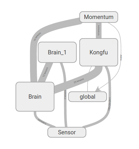
Figure 4: Computational graph of the simple neural network built for MNIST digit recognition example.

The underlying stories are described in the following section, which also debriefs the design motivation and vision behind akid.

akid is a kid who has the ability to keep practicing to improve itself. The kid perceives a data Source with its Sensor and certain learning methods (nicknamed KongFu) to improve itself (its Brain), to fulfill a certain purpose. The world is timed by a clock. It represents how long the kid has been practicing. Technically, the clock is the conventional training step.

To break things done, Sensor takes a Source which either provides data in form of tensors from Tensorflow or numpy arrays. Optionally, it can make jokers on the data using Joker, meaning doing data augmentation. The data processing engine, which is a deep neural network, is abstracted as a Brain. Brain is the name we give to the data processing system in living beings. A Brain incarnates one of data processing system topology, or in the terminology of neural network, network structure topology, such as a sequentially linked together layers, to process data. Available topology is defined in module systems. The network training methods, which are first order iterative optimization methods, is abstracted as a class KongFu. A living being needs to keep practicing Kong Fu to get better at tasks needed to survive.

A living being is abstracted as a Kid class, which assemblies all above classes together to play the game. The metaphor means by sensing more examples, with certain genre of Kong Fu(different training algorithms and policies), the data processing engine of the Kid, the brain, should get better at doing whatever task it is doing, letting it be image classification or something else.

3.2.2 Visualization

As a library gearing upon research, it also has rich features to visualize various components of a neural network. It has built-in training dynamics visualization, more specifically, distribution visualization on multi-dimensional tensors, e.g., weights, activation, biases, gradients, etc, and line graph visualization on on scalars, e.g., training loss, validation loss, learning rate decay, regularization loss in each layer, sparsity of neuron activation etc, and filter and feature map visualization for neural networks.

Distribution and scalar visualization are built in for typical parameters and measures, and can be easily extended, and distributedly gathered. Distribution visualizations are shown in Figure 5, and scalar visualizations are shown in Figure 6.

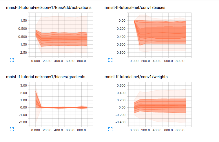
Figure 5: Visualization of how distribution of multi-dimensional tensors change over time. Each line on the chart represents a percentile in the distribution over the data: for example, the bottom line shows how the minimum value has changed over time, and the line in the middle shows how the median has changed. Reading from top to bottom, the lines have the following meaning: [maximum, 93%, 84%, 69%, 50%, 31%, 16%, 7%, minimum] These percentiles can also be viewed as standard deviation boundaries on a normal distribution: [maximum, $\mu$+1.5$\sigma$, $\mu$+$\sigma$, $\mu$+0.5$\sigma$, $\mu$, $\mu$-0.5$\sigma$, $\mu$-$\sigma$, $\mu$-1.5$\sigma$, minimum] so that the colored regions, read from inside to outside, have widths [$\sigma$, 2$\sigma$, 3$\sigma$] respectively.

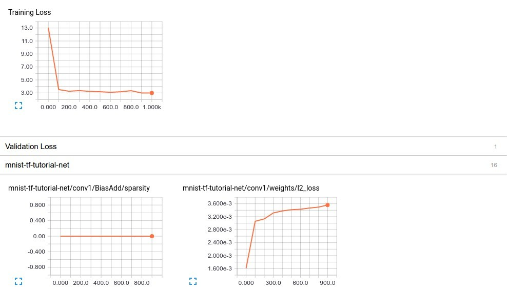
Figure 6: Visualization of how important scalar measures change over time.

akid supports visualization of all feature maps and filters with control on the layout through Observer class. When having finished creating a Kid, pass it to Observer, and call visualization as the following.

⬇

from akid import Observer

\paro = Observer(kid)

# Visualize filters as the following

o.visualize_filters()

# Or visualize feature maps as the following

o.visualize_activation()

Various layouts are provided when drawing the filters. Additional features are also available. The post-preprocessed visualization results of filters are shown in Figure 8, and that of feature maps are shown Figure 7.

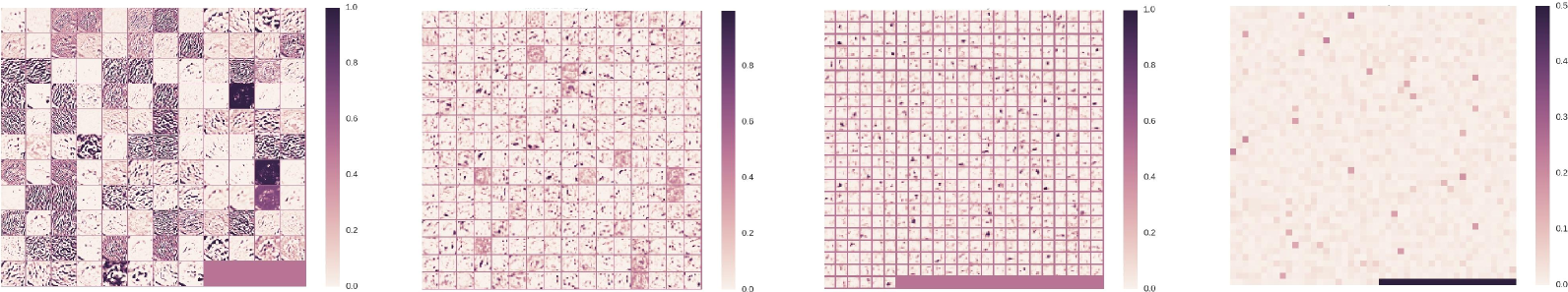
Figure 7: Visualization of feature maps learned.

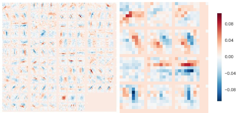
Figure 8: Visualization of filters learned.

3.3 Distributed Computation

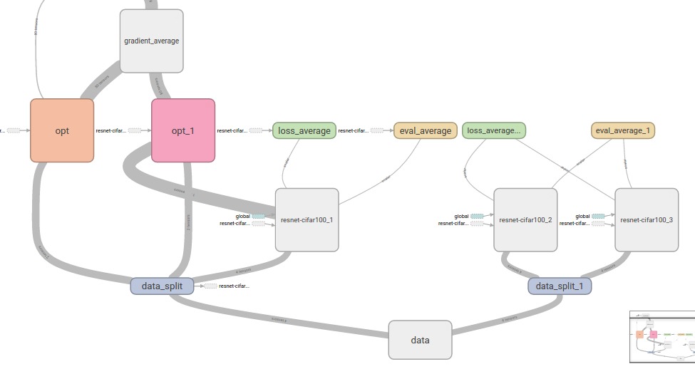
Figure 9: Illustration of computational graph constructed by a data parallel engine. It partitions a mini-batch of data into subsets, as indicated by the data_split blue blocks, and passes the subsets to replicates of neural network models at different computing towers, as indicated by the gray blocks one level above blue blocks, then after the inference results have been computed, the results and the labels (from the splitted data block) will be passed to the optimizers in the same tower, as indicated by red and orange blocks named opt, to compute the gradients. Lastly, the gradients will be passed to a tower that computes the average of the gradients, and pass them back to neural networks of each computing towers to update their parameters.

The distributed computing stack is responsible to handle concurrency and communication between different computing nodes, so the end user only needs to deal with how to build a power network. All complexity has been hidden in the class Engine. The usage of Engine is just to pick and use.

More specifically, akid offers built-in data parallel scheme in form of class Engine. Currently, the engine mainly works with neural network training, which is be used with Kid by specifying the engine at the construction of the kid.

As an example, we could do data parallelism on multiple towers using:

⬇

kid = kids.Kid(

sensor,

brain,

MomentumKongFu(

lr_scheme={

"name": LearningRateScheme.placeholder}),

engine={"name": "data_parallel", "num_gpu": 2},

log_dir="log",

max_epoch=200)

The end computational graph constructed is illustrated in Figure 9.

3.4 Distributed Deployment

The distributed deployment stack handles the actual production environment, thus decouples the development/prototyping environment and production environment. We leverage on recent developments of distributed system in the open source community to build a distributed deployment solution for akid. More specifically, we investigate and test out three cornerstone techniques that provides network file system, i.e. Glusterfs, containerization, i.e. Docker, and distributed scheduler, i.e. Kubernetes, functionality. More would come when we get the chance to test them out in a real production environment.

4 Conclusion

We have described akid, a neural network library that provides a four-layer stack to enable fast research prototyping and be production ready. It has a clean and intuitive application facing interface, nature inspired programming paradigm, and abstracts away distributing computing, decouples developments and operations.

References

- [1] B. Burns, B. Grant, D. Oppenheimer, E. Brewer, and J. Wilkes. Borg, Omega, and Kubernetes. Queue, 14(1):70–93, jan 2016.
- [2] T. Chen, M. Li, Y. Li, M. Lin, N. Wang, M. Wang, T. Xiao, B. Xu, C. Zhang, and Z. Zhang. MXNet: A Flexible and Efficient Machine Learning Library for Heterogeneous Distributed Systems. In NIPS, Workshop on Machine Learning Systems, dec 2016.
- [3] R. Collobert, R. Collobert, S. Bengio, and J. Marithoz. Torch: A Modular Machine Learning Software Library. Technical report, 2002.
- [4] J. D. J. Deng, W. D. W. Dong, R. Socher, L.-J. L. L.-J. Li, K. L. K. Li, and L. F.-F. L. Fei-Fei. ImageNet: A large-scale hierarchical image database. CVPR, 2009.
- [5] K. He, X. Zhang, S. Ren, and J. Sun. Delving Deep into Rectifiers: Surpassing Human-Level Performance on ImageNet Classification. In ICCV, 2015.
- [6] K. He, X. Zhang, S. Ren, and J. Sun. Identity Mappings in Deep Residual Networks. In ECCV, 2016.
- [7] Y. Jia, E. Shelhamer, J. Donahue, S. Karayev, J. Long, R. Girshick, S. Guadarrama, and T. Darrell. Caffe: Convolutional Architecture for Fast Feature Embedding. Technical report, jun 2014.
- [8] A. Krizhevsky, I. Sutskever, and G. E. Hinton. ImageNet Classification with Deep Convolutional Neural Networks. In NIPS, 2012.
- [9] S. Mallat. Understanding deep convolutional networks. Philosophical transactions. Series A, Mathematical, physical, and engineering sciences, 374(2065), 2016.
- [10] Merkel and Dirk. Docker: lightweight Linux containers for consistent development and deployment. Linux Journal, (239):2, 2014.
- [11] C. Szegedy, W. Zaremba, and I. Sutskever. Intriguing properties of neural networks. arXiv preprint arXiv: …, pages 1–10, 2013.
- [12] T. T. D. The Theano Development Team, R. Al-Rfou, G. Alain, A. Almahairi, C. Angermueller, D. Bahdanau, N. Ballas, F. Bastien, J. Bayer, A. Belikov, A. Belopolsky, Y. Bengio, A. Bergeron, J. Bergstra, V. Bisson, J. B. Snyder, N. Bouchard, N. Boulanger-Lewandowski, X. Bouthillier, A. de Brébisson, O. Breuleux, P.-L. Carrier, K. Cho, J. Chorowski, P. Christiano, T. Cooijmans, M.-A. Côté, M. Côté, A. Courville, Y. N. Dauphin, O. Delalleau, J. Demouth, G. Desjardins, S. Dieleman, L. Dinh, M. Ducoffe, V. Dumoulin, S. E. Kahou, D. Erhan, Z. Fan, O. Firat, M. Germain, X. Glorot, I. Goodfellow, M. Graham, C. Gulcehre, P. Hamel, I. Harlouchet, J.-P. Heng, B. Hidasi, S. Honari, A. Jain, S. Jean, K. Jia, M. Korobov, V. Kulkarni, A. Lamb, P. Lamblin, E. Larsen, C. Laurent, S. Lee, S. Lefrancois, S. Lemieux, N. Léonard, Z. Lin, J. A. Livezey, C. Lorenz, J. Lowin, Q. Ma, P.-A. Manzagol, O. Mastropietro, R. T. McGibbon, R. Memisevic, B. van Merriënboer, V. Michalski, M. Mirza, A. Orlandi, C. Pal, R. Pascanu, M. Pezeshki, C. Raffel, D. Renshaw, M. Rocklin, A. Romero, M. Roth, P. Sadowski, J. Salvatier, F. Savard, J. Schlüter, J. Schulman, G. Schwartz, I. V. Serban, D. Serdyuk, S. Shabanian, É. Simon, S. Spieckermann, S. R. Subramanyam, J. Sygnowski, J. Tanguay, G. van Tulder, J. Turian, S. Urban, P. Vincent, F. Visin, H. de Vries, D. Warde-Farley, D. J. Webb, M. Willson, K. Xu, L. Xue, L. Yao, S. Zhang, and Y. Zhang. Theano: A Python framework for fast computation of mathematical expressions. Technical report, may 2016.
- [13] W. Xiong, J. Droppo, X. Huang, F. Seide, M. Seltzer, A. Stolcke, D. Yu, and G. Zweig. Achieving Human Parity in Conversational Speech Recognition. Technical report, oct 2016.
- [14] M. Zeiler and R. Fergus. Visualizing and understanding convolutional networks. ECCV, 2014.