Testing for Equivalence of Network
Distribution Using Subgraph Counts
Abstract
We consider that a network is an observation, and a collection of observed networks forms a sample. In this setting, we provide methods to test whether all observations in a network sample are drawn from a specified model. We achieve this by deriving the joint asymptotic properties of average subgraph counts as the number of observed networks increases but the number of nodes in each network remains finite. In doing so, we do not require that each observed network contains the same number of nodes, or is drawn from the same distribution. Our results yield joint confidence regions for subgraph counts, and therefore methods for testing whether the observations in a network sample are drawn from: a specified distribution, a specified model, or from the same model as another network sample. We present simulation experiments and an illustrative example on a sample of brain networks where we find that highly creative individuals’ brains present significantly more short cycles than found in less creative people.
Keywords: Statistical Testing, Subgraph Count Statistics
1 Introduction
We show that subgraph counts are flexible and powerful statistics for testing distributional properties of networks, when more than one network is observed. Specifically, we use subgraph counts to test the hypotheses that all networks in a sample are generated either from a given distribution, from distributions specified by a given model class, or from the same model as that of another sample.
Our results address the fundamental inference problem raised by the following experiment (Gray et al., 2012): The networks connecting brain regions of individuals of varied levels of creativity are observed. However, while these observations can be assumed to be independent, due to the variability of the brain structure and the instability of the observation technique, they cannot be assumed to be identically distributed; for instance, they need not contain as many nodes and edges. Unfortunately, this implies that if we identify each network realization with its adjacency matrix, the obtained matrices will be of different sizes. This prevents, for instance, estimating the distribution the adjacency matrices are drawn from as one would from a sample of independent and identically distributed realizations. How, while allowing for such variations, can we test for significant differences between individuals with different levels of creativity?
Formally, we consider that each network is an observation—say for each subject—and a collection of observed networks form a sample—say . Then, our goal is to compare distributional properties of the -s as grows. This parallels more classical statistical settings, where an observation is a vector—such as —and a sample is a matrix: . However, this parallel with the classical setting stops there. Indeed, the need not be of the same size, or have nodes that are matched; i.e., the -s would not have the same dimension, and the entries could be shuffled.
This setting strongly differs from the two settings that have already seen extensive research. First, the setting where only one or two very large network are observed and for which many statistical tests already exist (see Hoff et al. (2012); Ho et al. (2012); Bickel et al. (2012); Sussman et al. (2012); Bhattacharyya and Bickel (2015); Tang et al. (2013); Olhede and Wolfe (2014); Fosdick and Hoff (2015); Klopp et al. (2016); Coulson et al. (2016), to cite but a few). Available statistical tests for network comparison in that setting focus on the case where one or two large networks are observed (Asta and Shalizi, 2014; Tang et al., 2017; Gao and Lafferty, 2017; Banerjee and Ma, 2017; Ghoshdastidar et al., 2017), or when one finite network is compared to a fixed model alone (Birmele, 2012; Ali et al., 2014, 2016). The second case addresses graph samples, as we do here, but under very restrictive assumptions: samples that are independent and identically distributed, where all graphs have the same size, and where nodes across networks can be matched one-to-one. Then, under these assumptions, it is possible to compare network summaries using classical statistical methods (Simpson et al., 2012; Stoffers et al., 2013; Daianu et al., 2013; Ginestet et al., 2017), or by fitting a parametric or semi-parametric model (Simpson et al., 2012; Wang et al., 2019; Durante and Dunson, 2018).
We provide, in the graph sample setting described above, an analog of the multivariate -test for network samples: methods to test whether a given network sample presents averages consistent with either a specific model, or with that of another sample. The averages we use are subgraph counts; e.g., the number of or in the sample. The choice of subgraph counts as statistics is motivated by their success in comparing large networks (Milo et al., 2002; Ali et al., 2014), but also by results in random graph theory and the study of large graphs. In both fields, subgraph counts have proved to be the most powerful tool available to compare networks (Ali et al., 2014, 2016) and are known to have properties similar to moments of random variables when studying large networks (Diaconis and Janson, 2008; Bickel et al., 2012; Lovász, 2012; Chatterjee and Diaconis, 2013). Finally, on account of these results, many powerful algorithm exists to count subgraphs efficiently; e.g., Talukder and Zaki (2016); Ortmann and Brandes (2016).
Formally, we are representing network samples in a space defined by subgraph counts, and performing comparisons in that space. While other network comparison techniques also use embeddings (Asta and Shalizi, 2014; Tang et al., 2017; Gao and Lafferty, 2017; Wang et al., 2019), using subgraph counts presents three key advantages: first, if the -s are generated by a blockmodel (Hoff et al., 2012)—one of the most popular random network models to date—and for some families of subgraphs, the embedding is one-to-one. This result is known as the finite forciblity of a family of graphs (Lovász, 2012, Ch. 16). Second, very few assumptions on each need to be made as grows to obtain consistency and asymptotic normality of the image of in the embedding space. This enables us to work under a very flexible null model. Finally, because it relies on direct summaries of the -s—the number of , , and so on—this embedding remains interpretable, part of the appeal to use subgraph based inference.
The main risk in subgraphs for testing purposes is that we cannot be assured that the subgraphs considered are sufficient to distinguish the null and the data generative mechanism. We provide several experiment allowing us to claim that while possible, this does not appear to be common. Furthermore, this risk is balanced by the interpretability of subgraph counts: if the null and the generative mechanism have the same number of subgraph, they are maybe equivalent for the purpose of the study at hand. Another shortcoming is that subgraph counts can be highly correlated, especially in denser networks, making the estimation of the inverse of their covariance matrix unstable. One of our contribution are closed form formulae for these covariance matrices under our null, which reduces but does not fully resolves this issue. Finally, because subgraph counting library are not standard, implementing the proposed methods is not as easy as for other methods, which tend to rely on more common, linear algebra related, data transformation pipelines. To this end we made all the code to perform our analysis available111Code to perform all methods, as well as reproduce all figure and tables reported in the article, can be found at: https://github.com/PierreAndreMaugis/motifs-for-network-samples.
In the remainder of this article, we first introduce subgraph counts and the kernel based random graph model. We then present, successively, the case where all the networks in the sample come from the same kernel model, and the case where each observed network may come from a different kernels. In both cases, we prove asymptotic normality of our estimator, present a plug-in estimator of its variance, describe the limit of the estimator under the alternative hypothesis, and provide representative examples showing the practical utility of the result. Methods to produce the figures, as well as supporting simulations, can be found in the Supplementary Material. We conclude with an analysis of connectome data, and with a discussion.
2 Subgraph Counts in Kernel Based Random Graphs
We now define our statistics (subgraph counts) and our null model (the kernel based random graph model). Subgraph counts are natural statistics to compare networks for two reasons. First, subgraph counts intuitively summarize a network through its fundamental building blocks. This has historically given them purchase to address hard fundamental and empirical problems (Rucinski, 1988; Milo et al., 2002; Ali et al., 2014). Second, subgraph counts present tractable analytical properties. We will describe and leverage these properties below, in a manner paralleling what is done in related literature (Bickel et al., 2012; Bhattacharyya and Bickel, 2015; Rucinski, 1988).
(a) (b) (c)
A subgraph count is the number of copies of a given graph in another graph (see Figure 1). Throughout, we call the subgraph—and denote —the graph which is counted and the larger graph in which the counting takes place. All graphs will be simple (unweighted, no self loops or multiple edges). Subgraphs are also termed motifs, pattern graphs or shapes depending on the field (Milo et al., 2002; Alon et al., 1997; Hočevar and Demšar, 2014; Benson et al., 2016).
For clarity, we define subgraph counts formally as follows:
Definition 1 (Graph equivalence ‘’).
Fix two graphs and . We say that is equivalent to—or is a copy of—, and write , if there exists a bijective map from the vertex set of to the vertex set of such that is an edge in iff is an edge in .
Definition 2 (Subgraph count ).
Fix two graphs and . We denote the number of non-necessarily induced subgraphs of equivalent to ; i.e,
where if the vertex end edge sets of are subsets of those of .
With this notation, calling , and the graphs in Figure 1, we have , , . A more complete definition is provided in Definition 2.
The power of subgraph counts to study networks stems from their inherent linearity. Indeed, products of subgraph counts are but linear combinations of other subgraph counts. Intuitively, first observe that a product of two subgraph counts will involve counting pairs of copies. Then, a product of subgraph counts can be recovered by counting the number of copies of all subgraphs that can be induced by a pair of copies. More precisely, in the Appendix we show the following, which is implicitly used in Rucinski (1988):
Lemma 1 (Linearity of subgraph counts (Rucinski, 1988)).
For any two graphs and , there are factors and a set of subgraphs—the set of subgraphs that can be obtained using one copy of each and as building blocks—such that for any graph
For instance, as these will be used later on, we have that in any graph ,
This algebraic property of subgraph counts allows us to understand the proofs of Rucinski (1988); Bhattacharyya and Bickel (2015). The property is also crucial to the subgraph counting algorithms of Hočevar and Demšar (2014), and can be found in many other examples. Crucially, as opposed to cases where the model enforces linearity—such as with assumptions of Normality—it is the nature of the statistics (subgraph counts) and the system (graphs) that makes the problem linear.
The linearity of subgraph counts allows us to use as null the very flexible kernel based model (Lovász, 2012). This framework subsumes most models used in the statistical literature on networks; e.g., blockmodel (Hoff et al., 2012) and dot-product models (Sussman et al., 2012). It has the intuitive structure of affixing to each node a latent feature (here ) and of connecting nodes and (conditionally independently) with a probability determined by the node features (here ).
Definition 3 (Kernel and random graph ).
Fix a symmetric measurable map , and call it a kernel. We call the random graph distribution over graphs with nodes such that: to each node is randomly and independently assigned a feature , with ; and where edges form independently conditionally on with conditional probability
To recover a blockmodel with blocks, it suffices to consider a partition of in sets (i.e., ) and set as constant over each . The dot-product model is recovered with a kernel of finite rank; i.e., .
The model assumes that vertices’ location in the latent space are independent and identically distributed, so that the model does not assume any structure or symmetry among the nodes in the observed networks. However, it can accommodate any such structure, which would be recovered through estimation. Nonetheless, in some cases it may seem relevant to enforce such structure; e.g., in our brain example, assume that nodes in different hemispheres are unlikely to connect. Doing so risks misspecifying the model to gain faster convergence, which might be necessary in some cases. We did not find it necessary in our application.
In the kernel framework, subgraph counts have direct interpretation as moments of (Lovász, 2012) (see 1). Specifically, if , then the moments of are moments of . An infinite number of subgraph counts are sufficient statistics to distinguish between any two kernel (Lovász, 2012; Bollobás and Riordan, 2009), as the subgraph counts can be used to define the subgraph metric. However, there are no guarantees on which or how many subgraph counts are needed to distinguish between two kernels. For blockmodels and finite rank models, we know only that a finite number is sufficient (a concept know as finite forcibility, see Lovász (2012, Chapter 16.7 & Appendix 4) for more details).
This makes subgraph counts especially appropriate as statistics in an hypothesis test. Indeed, for any finite set of subgraphs , we could have two kernels and such that , and yet . However, as we prove below, if for any , then . Therefore, a difference in subgraph counts is sufficient but not necessary to distinguish between kernels. Conversely, not observing a difference in subgraph count can only imply that we do not observe a difference in the kernels, and therefore that we fail to reject the hypotheses that the kernel are equal. This has implication regarding the power of our test that we explore below.
Unfortunately, all known results on subgraph counts under the kernel model consider the setting where one very large graph is observed. Here we present the tools to address the problem where a sample of graphs is observed.
3 The simple case: Samples from one kernel
We now present a central limit theorem as well as practical methods to build confidence regions for the subgraph counts observed in a network sample . In this section, we assume that there is a kernel such that each is drawn independently from (with , where for any graph we write for the number of nodes in ).
Fix and . In this setting, is a random variable, and the first parameter to consider is its mean. To compute this mean, let be all the copies of in (the complete graph over the nodes of ), so that using the linearity of the expectation, we have that
Then, direct computations show that does not depend on (see Proposition 1), and that
| (1) |
so that . Observe that is a moment of the kernel , as discussed above.
Similar computations for higher moments, aided by Lemma 1, enable us to use the Lindeberg-Feller central limit theorem and the Cramer-Wold device to prove the following:
Theorem 1 (Statistical properties of subgraph counts).
Fix a set of graphs , a kernel and a sequence such that . Let be a network sample such that for all , . Set , , and . Then, is an unbiased, -consistent and asymptotically normal estimator of ; i.e., and there exists a positive semi-definite such that asymptotically in :
Furthermore, for each ,
| (2) |
with the disjoint union of , , and is defined in Lemma 1.
Crucial to the following is the covariance matrix —which can be obtained by taking the limit in in (2) for each —and which will enable the computation of confidence regions. Interestingly, its elicitation is more involved than for the study of large networks, where only a few terms dominate. We refer to the Appendix for the proof. The Appendix’s proof relies on understanding the moments of single network counts, which have been studied extensively in the Erdős–Rényi and the exchangeable cases, see for example Rucinski (1988); Coulson et al. (2016).
Remark 1 (Non-random latent positions).
Because our proof build on the foundation of Rucinski (1988), our results extend to the case where the latent -s are not random; say fixed to some values. The only modification would be that the sum in (2) should be restricted to graphs formed by copies of and overlapping over at least an edge (as opposed to overlapping over one node in (2).) This also means that all our methods apply to that case, with the caveat that the resulting test will be conservative (as the variance is overestimated.)
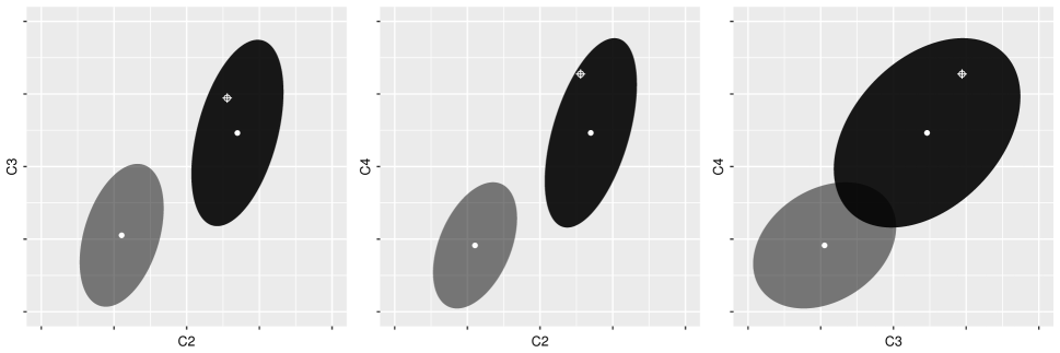
Theorem 1 enables testing against the null that all are drawn from a given kernel. Further, the Appendix contains a simulation experiment exploring convergence in small sample. To make this concrete, we consider an example in Figure 2. There, we observe a graph sample , and aim to compare it to two kernels (in black) and (in gray) using Theorem 1; i.e., we assume that for , and consider the null hypothesis and the alternative . We draw as a white cross . The sizes of the networks in , the , are non-random but not constant. We achieve this by using the sequence of digits of .
First, since we have specified and , we can evaluate both and and draw them on the figure (as white dots). Then, since is observed, we can compute and using Theorem 1, which allows us to compute the confidence ellipse around and (in shaded black and gray respectively). Finally, since we know the limit distribution and covariance under the null, we can use and to compute a -value using Mahalanobis distance; e.g., assuming is full rank, the -value is , with the cumulative distribution function of the distribution with degrees of freedom.
Figure 2 is useful to understand the power of the proposed test. We see that since all the confidence ellipses do not all overlap, the power is larger than . However, if we were to use only and , then the power would be less as the ellipses overlap. For larger sample sizes, the radii of both ellipses will be smaller, so that eventually the power tends to using any combination of subgraphs. In the Supplementary Material we explore the power of our test when the expected count is held fixed, but the number of blocks in the null and true models differ.
In the following we consider the case where instead of testing against the null of a single kernel, we test against the null of a kernel class.
4 The general case: Flexible sampling design
Here we expand our results to cases where the observed networks may be generated from different kernels. Indeed, in many settings, the sampling mechanism may distort the structure of the underlying kernel; e.g., although the network connecting brain regions can be satisfactorily modeled by a blockmodel (Koutra et al., 2013), the proportion of nodes of each block may be different in different experimental settings, so that each observation is drawn from a different blockmodel.
In this practically important and conceptually challenging new setting, the proof techniques developed for Theorem 1 yield the following.
Theorem 2.
Fix a set of graphs , a sequence of kernels and a sequence of integers such that . Let be a network sample such that for all , . Set and . Then, asymptotically in , and for some , we have
Therefore, even in this much more flexible setting, we can recover the barycenter of the . However, the variance has now a more complex structure (see Appendix for details).
Following the intuition of our example of brain networks, and to make the usefulness of Theorem 2 concrete, we introduce the flexible stochastic blockmodel (FSBm).
Definition 4 (FSBm and embedding shape).
For a symmetric matrix we call the set of all possible kernels with the same block structure as ; i.e., recalling that is the set of partitions of in sets,
For a set of graphs, we call embedding shape the set
For instance, with and , then:
The most direct way of using the FSBm is to test for all the being equal to any blockmodel instance in a class; i.e assume that all -s are drawn from a kernel and test for the null . This is achieved by using a composite hypothesis test, and our results allow us to produce confidence regions and -values using the same tools as before.
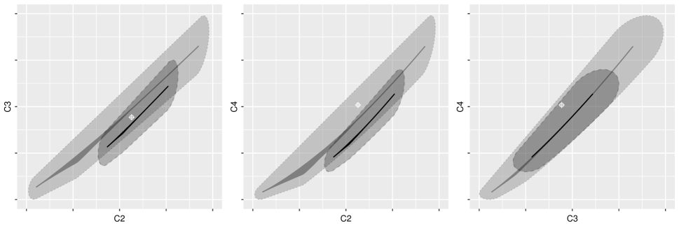
We present such an example in Figure 3. There, we observe , and consider two FSBm classes generated from (in gray) and (in black). Then, we assume that all networks in the sample are drawn from a kernel and test for the null and the alternative . We first represent as a white cross. Using Definition 4, we plot the embedding shapes and in solid gray and black respectively. The confidence regions (in shaded gray with dotted contour and black with dashed contour) are the union of the confidence ellipses at all points in and .
A more general use of Theorem 2 is to test for all graphs in a sample being drawn from elements of a FSBm class; i.e assume that the -s are drawn from the -s and test for the null for some . As before, we face a composite null, and we may compute the confidence region and the -value by scanning all possible sequences . This, however, is clearly computationally intractable. Nonetheless, the form of the variance and the structure of the FSBm allows us to propose conservative confidence regions and -values that can be efficiently computed (we fully describe the method in the Supplementary Information).
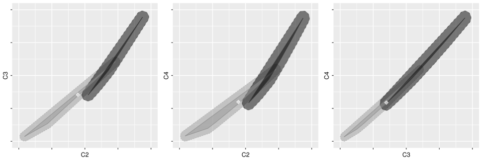
We present an example in Figure 4. There we observe and consider two FSBm classes generated by and . We first plot as a white cross. Then, using Definition 4, we plot the convex hull of the embedding shapes and (in solid gray and black respectively) wherein—by Theorem 2— must lie. Finally, we use a method described in the SI to produce the confidence region around each shape (in shaded hue).
5 Are creative brains different from less creative ones?
We now consider a sample of brain networks (Koutra et al., 2013). This sample was produced as follows: diffusion MRI (dMRI) and structural MRI (sMRI) scans from individuals were collected over sessions from Beijing Normal University (Zuo et al., 2014). Graphs were estimated using the ndmg (Kiar et al., 2018) pipeline. The dMRI scans were pre-processed for eddy currents using FSL’s eddy-correct (Smith et al., 2004). FSL’s “standard” linear registration pipeline was used to register the sMRI and dMRI images to the MNI152 atlas (Woolrich et al., 2009; Jenkinson et al., 2012; Mazziotta et al., 2001). A tensor model is fit using DiPy (Garyfallidis et al., 2014) to obtain an estimated tensor at each voxel. A deterministic tractography algorithm is applied using DiPy’s EuDX (Garyfallidis et al., 2012) to obtain streamlines, which indicate the voxels connected by an axonal fiber tract. Simple graphs are formed by first contracting voxels into graph vertices according to the Desikan parcellation (Desikan et al., 2006) and then by placing an edge between two regions if a fiber tract is observed between any pair of voxel from each regions. Further, we have available a covariate measuring subject’s creativity, which is related to the person’s performance on a series of creativity tasks.
To study this network sample and use the covariate , we introduce a direct extension of our results to compare two network samples:
Corollary 1 (Two-sample test).
Fix a set of subgraphs and two network samples and generated respectively by the kernels and and the network size sequences and . Then, as both and tend to infinity, and if , we have that if , then
and, as (2) applies, we can produce an unbiassed -consistent and asymptotically normal estimator of , this without specifying or estimating .
In the following we choose to work with . We chose these for several reasons: in a simulation experiment (see Supplementary Material) we find that using these counts leads to power surpassing the best available alternative in the literature (Tang et al. (2017), Tang et al. (2017)); the associated counts correspond to spectral moments of the underlying kernel (Maugis et al., 2017b); and are staples of graph analysis (related to conductance, clustering, transitivity, …) and are key network summaries throughout the literature; is one of the smallest graphs that is larger than and but cannot be built from copies of and , which reduces correlation between counts, and therefore improve power of the tests; all three are small, and there is extensive and available software to efficiently count them (e.g., Maugis et al. (2017a); Jha et al. (2015); Pinar et al. (2016).)
We note that our estimator of is entrywise Normal, not Wishart as in the classical setting. Thus, we have no guarantee that is positive definite, and cannot use the Hotelling’s -squared distribution to compute -values. If the estimate is positive definite, we recommend ignoring the variations in and using the distribution. If the estimate is not positive definite, we recommend using the marginals.
Before analyzing using our results, we make the following test: we subsample uniformly at random and without replacement from , yielding and such that , and use Corollary 1 to test for and being drawn from the same kernel . Unless presents characteristics that cannot be explained by our results, and should be indistinguishable, and we expect to see -values that are uniformly distributed in .
We perform this experiment times, and obtain a sample of -values for which we fail to reject the null of a uniform distribution using the Kolmogorov–Smirnov test (, -value ). For this test we use because of the small sample () size and a very high level of correlation; otherwise the correlation between the counts is so high that the correlation matrix appears singular.
We now use to split in two samples. To do so, we choose to build a first subsample containing the less creative, and a second subsample containing the more creative. More precisely, for a quantile and denoting the empirical quantile function of :
Interestingly, for and , we fail to reject the null that the networks in and come from the same kernel (see Table 3 for the -values). However, for we can reject the null of the same kernel at the confidence level using or , but not .
| Quantile () | -value | ||
|---|---|---|---|
| | | | |
| 0.5 | 0.126 | 0.110 | 0.115 |
| 0.4 | 0.077 | 0.051 | 0.050 |
| 0.3 | 0.062 | 0.042 | 0.040 |
| 0.2 | 0.014 | 0.011 | 0.012 |
| 0.1 | 0.046 | 0.047 | 0.061 |
Thus, we observe that individuals with a very high level of creativity present significantly more and than those with a very low level of creativity. To further confirm this discovery, we undertake the following experiment: we estimate kernels (through the random-dot-product framework (Athreya et al., 2018)) over the samples , , and , that we call , , and respectively; then, for several , we consider the power of Corollary 1’s test when the samples compared are of the same cardinality as , and , but drawn i.i.d. from and respectively; we find that the proposed test is very powerful, as powerful than a semi-parametric test relying on the random-dot-product structure of the model (Tang et al., 2017). This comforts the claim that the difference in sample is only observed for , and not for more central quantiles.
We now aim to understand whether the added and arise from a few edges completing partially present shapes or from fully new and . To do so, we first observe that if , then , where is the complement graph of . Therefore, we may use our tests on , which can be understood as estimating instead of to compare network samples.
Then, using the , we can test whether there are significantly more fully absent subgraphs in compared to . There, we find we cannot reject this null; i.e., we cannot reject the null of the networks in and coming from the same kernel for . Therefore, we conclude that the added and in the highly creative arise from a few edges completing partially present and .
One key conclusion of our analysis is that we must use Theorem 2 to study . Indeed, we have just shown that all networks generating cannot come from the same kernel. This allows us to write, that using the full sample , a centered and consistent estimate of the average density of within human brains is . To conclude, we remark that since all the s in have the same number of nodes, one could produce a similar analysis using—instead of our results—the as if they formed an independent and identically distributed sample. However, as we have just shown, the are not identically distributed, and therefore such an analysis could lead to spurious conclusions.
6 Discussion
We provide the tools to perform statistical inference on a network sample using subgraph counts. Our two main results provide consistency and asymptotic normality of subgraph counts under very flexible conditions. Using these results, we show that subgraph counts are powerful statistics to test whether network samples come from a specified distribution, a specified model, or from the same model.
The key insight we provide is that statistical inference methods paralleling classical ones for standard samples may be obtained for network samples. From this perspective, our results may be seen as providing an analog of a multivariate -test for network samples. However, going beyond what our results directly imply, we expect that parallels to ANOVA, model selection, model ranking, and goodness of fit may be obtained for network samples using our proof techniques.
However, since our tests are analog to the -test, they rely on global summaries. Therefore, while we can reject the null of two network samples being drawn from the same model, our approach is unable to locate where in the network the difference is stemming from.
Appendix A Properties of subgraph counts
In the following we formalize certain notions we use loosely in the main body (especially the notion of copy and the sets , as well as the constants ), prove all our results, and provide more details on the numerical examples we present.
We start by proving our first lemma, establishing the linearity of subgraph counts. We first define and , generalizing definitions given in Rucinski (1988).
Definition 5 (Overlapping copies).
For two graphs and we write the set of unlabeled graphs that can be formed by two copies of and , and the number of ways a given can be built from copies of and :
Finally, call the set removed of , the vertex disjoint union of and .
Note that is defined as a quotient set, sometimes called quotient space, through the equivalence relation . In the following we identify the equivalence classes in with any of their element, and therefore will treat the elements of as graphs.
Lemma 2 (Copies pairwise interaction).
Fix three graphs and . Then,
Proof.
We start by writing:
| (3) |
Now, from Definition 5, we first note that by construction of , for each pair in the sum, if and only if there exists such that . Therefore we can reindex the sum in (3) as follows:
We now note that by definition of , for each copy of in , there will be pairs of copies of and in such that . Therefore we can simplify the sum above to obtain:
yielding the desired result. ∎
With these tools in hand, we compute the first two moments of when .
Proposition 1.
Fix two graphs and and a random graph such that . Then, we have that
Proof.
We prove each statement in succession. To begin, call the copies of in ( because ). Then, and by linearity of the expectation,
| (4) |
Let us fix and consider . To do so we will use the law of total probability:
Therefore, does not depend on , and resuming from (4), we obtain
| (5) |
which is the desired result.
We now turn to the variance. Call the copies of in ( because ). We first write that
| (6) |
Now, we observe that if is disjoint form (i.e., which is possible because ) then is independent from and we have that
Therefore resuming from (6) we obtain that
Then, by the exact same transformation we used in Lemma 2, we know that each is in (because they are not disjoint), and furthermore, for each copy of in there are pairs and such that , so that
which is the desired result. ∎
We now turn to the proofs of Theorems 1 and 2. As the second generalizes the first, it is sufficient to prove the second.
Proof.
We obtain the result by a joint application of the Lindeberg-Feller central limit theorem and the Cramer-Wold device. To do so, we fix and compute the variance of our estimator projected along .
Computing the variance: First recall that Therefore, denoting “” the inner product and taking the expectation over , let
Then, using the independence of the s and the bi-linearity of the covariance, we have
To proceed, recall that for each , . Then, we may use Proposition 1 to obtain
Because all sums are finite, we can reorder the summations, leading to
| (7) |
where
Convergence of : To proceed we must show that converges to a limit as diverges. We will achieve this by showing that is Cauchy. To do so, observe that
Then, we recall that (see for instance Bollobás and Riordan (2009)), where is the number of automorphisms of (the number of bijections from the vertex set of to itself that preserve adjacency.) Then, as , we have
As furthermore is bounded by , we have leading to for . Thus, the sequence is Cauchy, and we may call its limit; i.e.,
Satisfying the Lindeberg-Feller condition: To invoke the Lindeberg-Feller central limit theorem, we must show that our sequence verifies the so called Lindeberg-Feller condition. Recall that the sequence under study is
and that the variance of the partial sum is . Therefore, the Lindeberg-Feller condition we need to satisfy is the following:
| (8) |
To verify the condition we first fix . Then, observe that since for each and we have and , we have that by the triangle inequality. Therefore, as as grows, we may fix an such that for all we have . In this setting, the sum in (8) is equal to zero for all , and the condition is verified. Therefore, we have that
Reverting to the notation of the statement of the Theorem, we have that for any
which is sufficient to obtain the claimed result for the limit in distribution. ∎
We now turn to the proof of Corollary 1.
Proof.
The result follows almost immediately from Theorem 1 and Slutsky’s theorem.
First, since and tend to infinity and both and are large enough, we have
As both samples are independent, linear combinations are also multivariate Gaussian. Therefore, multiplying the first line by , the second by (both ratios being in , the limit in distribution is unaffected), and taking the difference, we obtain, with
which is the desired limit in distribution.
To obtain the consistent estimator of we first recall that for
Then, with we have
There observe that:
-
–
As and grow we have that
-
–
All the in may be estimated by Furthermore, both and may be estimated in the same way.
Then, by a direct application of the Slutsky’s theorem, we have that
is an asymptotically normal estimator of converging at rate , which yields the claimed result. ∎
Appendix B Finite sample experiments
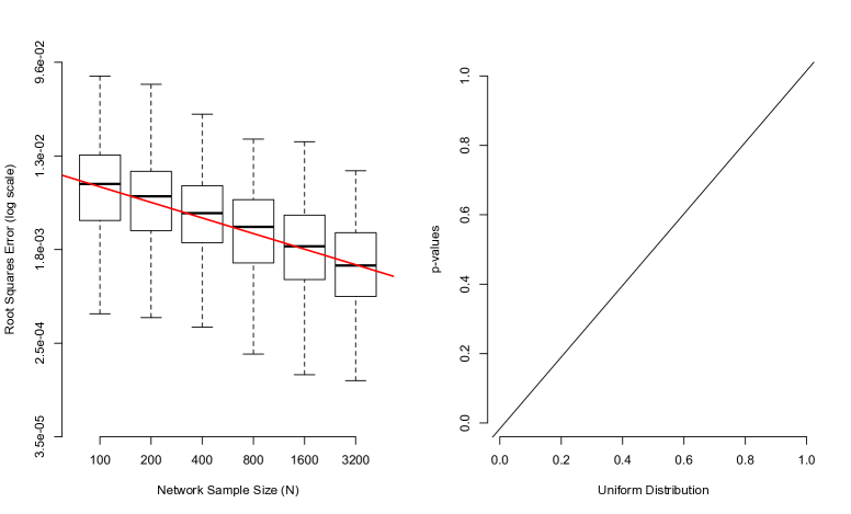
Before we proceed, we consider a simulation experiment to determine how large the sample size must be for the asymptotic limit to be a satisfactory approximation of the statistic’s distribution. We present our result in Figure 5. There, we observe that fairly small , on the order of 100 even with small -s, may be sufficient. Furthermore, results from Bickel et al. (2012) suggest that larger networks would make this convergence faster.
Appendix C Power experiments
C.1 Direct application of Theorem 1
Here we consider the simple problem where we test for a sample being drawn from a given model, as in Figure 2.
Specifically we first fix and consider the following family of blockmodels : graphs over vertices and equisized blocks, of fixed global density , and where between blocks probability of connection is , and within blocks probability of connection is constant (set to that the overall density is .)
Then, for to , we draw graphs from , yielding . This enables us to investigate the power of our test. Specifically we estimate the probability to reject when we test for the null of for . To obtain power estimates, we apply Theorem 1 with a level of .05 over 5000 replicates, yielding the following table:
| Sample name | Null model | ||
|---|---|---|---|
| 0.047 | 0.108 | 0.460 | |
| 0.332 | 0.053 | 0.091 | |
| 0.754 | 0.232 | 0.058 | |
C.2 Direct application of Corollary 1
Resuming from the main document, Section 5. We undertake the following experiment: we estimate kernels (through the random-dot-product framework (Athreya et al., 2018)) over the samples , , and , that we call , , and respectively; then, for several , we consider the power of Corollary 1’s test when the samples compared are of the same cardinality as , and , but drawn i.i.d. from and respectively.
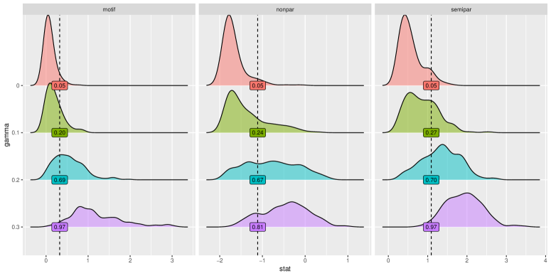
The purpose of the exercise is to see how large needs to be for the tests to show reasonably good power. But also to compare the powers of the test to other in the literature. Specifically, we compare to both Tang et al. (2017) and Tang et al. (2017). These tests are tightly related to that of Durante and Dunson (2018). Call , and the respective power of our test, that of Tang et al. (2017) and that of Tang et al. (2017) respectively. Then, we observe that:
| -test outcomes (at ) under the null that | ||
|---|---|---|
| 0.1 | Fail to reject | Fail to reject |
| 0.2 | Fail to reject | Fail to reject |
| 0.3 | Fail to reject | Reject |
Appendix D Methods to produce Figures 2-4
The code to produce all figures and tables is available from the authors. All computation are done in R. To ease presentation we always denote the number of blocks in the blockmodel, or flexible blockmodel, under consideration. Furthermore, we call the -th digit of .
D.1 Subgraph counting
D.2 Figure 2
We first describe the network sample. The sample is such that for each , , where , , and .
We now describe the construction of the confidence region and -value under the null. The first task is to compute the subgraph densities (the and ). To do so, we use the formulas presented in Coulson et al. (2016); Bickel et al. (2012) to compute subgraph densities in the blockmodel. More specifically, they show that for a kernel blockmodel with blocks such that the probability of being in each block is , and the block matrix is , then
Practically, this is achieved by imbricated loops.
That we can compute the subgraph densities under the null directly implies that we can compute both and . Then, the construction of the confidence ellipse as well as of the -value using the Mahalanobis distance are classical statistical inference methods which we need not describe here.
The black region is built with . The gray region is built with where , , and
D.3 Figure 3
We first describe the network sample. The sample is such that for each , , where for , , and
We now describe how we produced the embedding shape and its confidence region. First, to produce the embedding shape, we compute for a a large number of elements of . Practically, we parametrize by a -dimensional vector , the entries of which are the sizes of each block, and call the associated kernel . Then, we build a grid over the dimensional simplex of step-size , and for each we compute . To produce the confidence region, we produce the confidence ellipse for each which we achieve by computing for each in our grid .
The gray region is built with . The black region is built with where, for , , and
D.4 Figure 4
We first describe the network sample. The sample is such that independently for each , , where is drawn uniformly at random over with for , , .
We now describe how we produced the surface where may live as well as its confidence region. First, we know that may realize any point in the convex hull of the embedding shape. Therefore, we build the embedding shape as for Figure 3, and then present its convex hull. Building the confidence region is achieved using the following reasoning:
-
–
Observe that for any kernel and , . This can for instance be directly recovered from the formulas in Proposition 1. Then, for any sequences and , we have that , so that all correlations are positive, and the greatest amplitude of the confidence ellipse will be found on its first quadrant; i.e., the variance of will be maximal for some such that for all .
-
–
For any sequences and , we have that
Then, for any in the first quadrant we have that . Therefore, the maximal radius of the ellipse associated with on the first quadrant is larger than that induced by . Thus, by the previous item, the maximal radius of is larger than that of . It follows that the auxiliary sphere of the ellipse associated with contains that associated with .
-
–
Finally, is dominated by , where is the constant kernel equal to the maximal entry of . In this final setting, we need only compute the , where describes an Erdős-Rényi random graph. This makes the computation straightforward as we then have , where is the number of edges in .
Following this argument, our confidence region is the union of the auxiliary spheres of the ellipse associated with centered at each point in the convex hull of the embedding shape. Finally, the gray region is built with , where for , , .
References
- Ali et al. (2014) Ali, T., T. Rito, G. Reinert, F. Sun, and C. M. Deane (2014). Alignment-free protein interaction network comparison. Bioinformatics 30, i430–i437.
- Ali et al. (2016) Ali, W., A. E. Wegner, R. E. Gaunt, C. M. Deane, and G. Reinert (2016). Comparison of large networks with sub–sampling strategies. Scientific Reports 6, 28955.
- Alon et al. (1997) Alon, N., R. Yuster, and U. Zwick (1997). Finding and counting given length cycles. Algorithmica 17(3), 209–223.
- Asta and Shalizi (2014) Asta, D. and C. R. Shalizi (2014). Geometric network comparison. arXiv:1411.1350.
- Athreya et al. (2018) Athreya, A., D. E. Fishkind, K. Levin, V. Lyzinski, Y. Park, Y. Qin, D. L. Sussman, M. Tang, J. T. Vogelstein, and C. E. Priebe (2018). Statistical inference on random dot product graphs: a survey. JMLR 18, 1–92.
- Banerjee and Ma (2017) Banerjee, D. and Z. Ma (2017). Optimal hypothesis testing for stochastic block models with growing degrees. arXiv:1705.05305.
- Benson et al. (2016) Benson, A. R., D. F. Gleich, and J. Leskovec (2016). Higher-order organization of complex networks. Science 353(6295), 163–166.
- Bhattacharyya and Bickel (2015) Bhattacharyya, S. and P. J. Bickel (2015). Subsampling bootstrap of count features of networks. Ann. Statist. 43, 2384–2411.
- Bickel et al. (2012) Bickel, P. J., A. Chen, and E. Levina (2012). The method of moments and degree distributions for network models. Ann. Statist. 39, 2280–2301.
- Birmele (2012) Birmele, E. (2012). Detecting local network motifs. E. J. Stat. 6, 908–933.
- Bollobás and Riordan (2009) Bollobás, B. and O. Riordan (2009). Metrics for sparse graphs. In S. Huczynska, J. D. Mitchell, and C. M. Roney-Dougal (Eds.), Surveys in Combinatorics 2009, pp. 211–287. Cambridge, UK: Cambridge University Press.
- Chatterjee and Diaconis (2013) Chatterjee, S. and P. Diaconis (2013). Estimating and understanding exponential random graph models. Ann. Statist. 41(5), 2428–2461.
- Coulson et al. (2016) Coulson, M., R. E. Gaunt, and G. Reinert (2016). Poisson approximation of subgraph counts in stochastic block models and a graphon model. arXiv:1509.07754.
- Daianu et al. (2013) Daianu, M., N. Jahanshad, T. Nir, A. Toga, C. Jack, M. Weiner, and P. Thompson (2013). Breakdown of brain connectivity between normal aging and alzheimer’s disease: A structural k-core network analysis. Brain Connectivity 3, 407–422.
- Desikan et al. (2006) Desikan, R., F. Segonne, B. Fischl, B. Quinn, B. Dickerson, D. Blacker, R. Buckner, A. Dale, R. Maguire, B. Hyman, M. Albert, and R. Killiany (2006). An automated labeling system for subdividing the human cerebral cortex on mri scans into gyral based regions of interest. NeuroImage 16530430, 1053–8119.
- Diaconis and Janson (2008) Diaconis, P. and S. Janson (2008). Graph limits and exchangeable random graphs. Rendi. Mat. Appl. 28, 33–61.
- Durante and Dunson (2018) Durante, D. and D. B. Dunson (2018). Bayesian inference and testing of group differences in brain networks. Bayesian Anal. 13, 29–58.
- Fosdick and Hoff (2015) Fosdick, B. and P. D. Hoff (2015). Testing and modeling dependencies between a network and nodal attributes. J. Amer. Statist. Assoc. 110(511), 1047–1056.
- Gao and Lafferty (2017) Gao, C. and J. Lafferty (2017). Testing network structure using relations between small subgraph probabilities. arXiv:1704.06742.
- Garyfallidis et al. (2014) Garyfallidis, E., M. Brett, B. Amirbekian, A. Rokem, S. Van Der Walt, M. Descoteaux, and I. Nimmo-Smith (2014). Dipy, a library for the analysis of diffusion mri data. Frontiers in neuroinformatics 8, 8.
- Garyfallidis et al. (2012) Garyfallidis, E., M. Brett, M. Correia, G. Williams, and I. Nimmo-Smith (2012). Quickbundles, a method for tractography simplification. Frontiers in neuroscience 6, 175.
- Ghoshdastidar et al. (2017) Ghoshdastidar, D., U. von Luxburg, M. Gutzeit, and A. Carpentier (2017). Two-sample tests for large random graphs using network statistics. arXiv:1705.06168.
- Ginestet et al. (2017) Ginestet, C. E., J. Li, P. Balachandran, S. Rosenberg, and E. D. Kolaczyk (2017). Hypothesis testing for network data in functional neuroimaging. Ann. Appl. Stat. 11, 725–750.
- Gray et al. (2012) Gray, W. R., J. A. Bogovic, J. T. Vogelstein, B. A. Landman, J. L. Prince, and R. J. Vogelstein (2012). Magnetic resonance connectome automated pipeline: an overview. IEEE pulse 3(2), 42–48.
- Ho et al. (2012) Ho, Q., A. P. Parikh, and E. P. Xing (2012). A multiscale community blockmodel for network exploration. J. Amer. Statist. Assoc. 107(499), 916–934.
- Hoff et al. (2012) Hoff, P. D., A. E. Raftery, and M. S. Handcock (2012). Latent space approaches to social network analysis. J. Amer. Statist. Assoc. 97(460), 1090–1098.
- Hočevar and Demšar (2014) Hočevar, T. and J. Demšar (2014). A combinatorial approach to graphlet counting. Bioinformatics 30, 559–565.
- Jenkinson et al. (2012) Jenkinson, M., C. Beckmann, T. Behrens, W. M., and S. S. (2012). FSL. NeuroImage 62(2), 782–90.
- Jha et al. (2015) Jha, M., C. Seshadhri, and A. Pinar (2015). Path sampling: A fast and provable method for estimating 4-vertex subgraph counts. In Proceedings of the 24th International Conference on World Wide Web, WWW ’15, New York, NY, USA, pp. 495–505. ACM.
- Kiar et al. (2018) Kiar, G., E. Bridgeford, W. Roncal, C. f. R. (CoRR), Reproducibliity, V. Chandrashekhar, D. Mhembere, S. Ryman, X. Zuo, D. Marguiles, R. Craddock, C. Priebe, R. Jung, V. Calhoun, B. Caffo, R. Burns, M. Milham, and J. Vogelstein (2018). A high-throughput pipeline identifies robust connectomes but troublesome variability. bioRxiv, 188706.
- Klopp et al. (2016) Klopp, O., A. B. Tsybakov, and N. Verzelen (2016). Oracle inequalities for network models and sparse graphon estimation. Ann. Statist. 45, 316–354.
- Koutra et al. (2013) Koutra, D., J. T. Vogelstein, and C. Faloutsos (2013). DeltaCon: A principled massive-graph similarity function. In Proceedings of the SIAM International Conference in Data Mining. Society for Industrial and Applied Mathematics, pp. 162–170. SIAM.
- Lovász (2012) Lovász, L. (2012). Large Networks and Graph Limits. Providence, RI: Am. Mathematical Soc.
- Maugis et al. (2017a) Maugis, P.-A. G., S. C. Olhede, and P. J. Wolfe (2017a). Fast counting of medium-sized rooted subgraphs. arXiv:1701.00177.
- Maugis et al. (2017b) Maugis, P.-A. G., S. C. Olhede, and P. J. Wolfe (2017b). Topology reveals universal features for network comparison. arXiv:1705.056777.
- Mazziotta et al. (2001) Mazziotta, J., A. Toga, A. Evans, P. Fox, J. Lancaster, K. Zilles, R. Woods, T. Paus, G. Simpson, B. Pike, C. Holmes, L. Collins, P. Thompson, D. MacDonald, M. Iacoboni, T. Schormann, K. Amunts, N. Palomero-Gallagher, S. Geyer, L. Parsons, K. Narr, N. Kabani, G. Le Goualher, J. Feidler, K. Smith, D. Boomsma, P. Hulshoff, T. Cannon, R. Kawashima, and B. Mazoyer (2001). A four-dimensional probabilistic atlas of the human brain. Journal of the American Medical Informatics Association 8, 401–430.
- Milo et al. (2002) Milo, R., S. Shen-Orr, S. Itzkovitz, N. Kashtan, D. Chklovskii, and U. Alon (2002). Network motifs: Simple building blocks of complex networks. Science 298, 824–827.
- Olhede and Wolfe (2014) Olhede, S. C. and P. J. Wolfe (2014). Network histograms and universality of blockmodel approximation. Proc. Natl. Acad. Sci. USA 111, 14722–14727.
- Ortmann and Brandes (2016) Ortmann, M. and U. Brandes (2016). Quad census computation: simple, efficient, and orbit-aware, pp. 1–13. Cham: Springer Int. Publishing.
- Pinar et al. (2016) Pinar, A., C. Seshadhri, and V. Vishal (2016). Escape: Efficiently counting all 5-vertex subgraphs. arXiv:1610.09411.
- Rucinski (1988) Rucinski, A. (1988). When are small subgraphs of a random graph normally distributed? Probab. Theory Related Fields 78(1), 1–10.
- Simpson et al. (2012) Simpson, S., M. Moussa, and P. Laurienti (2012). An exponential random graph modeling approach to creating group-based representative whole-brain connectivity networks. NeuroImage 60, 1117–1126.
- Smith et al. (2004) Smith, S., M. Jenkinson, M. Woolrich, C. Beckmann, T. Behrens, H. Johansen-Berg, P. Bannister, M. De Luca, I. Drobnjak, D. Flitney, R. Niazy, J. Saunders, J. Vickers, Y. Zhang, N. De Stefano, J. Brady, and P. Matthews (2004). Advances in functional and structural mr image analysis and implementation as fsl. NeuroImage 23, S208–19.
- Stoffers et al. (2013) Stoffers, D., H. Berendse, K. Olde Dubbelink, A. Hillebrand, C. Stam, J. Deijen, and J. Twisk (2013). Disrupted brain network topology in parkinson’s disease: a longitudinal magnetoencephalography study. Brain 137, 197–207.
- Sussman et al. (2012) Sussman, D. L., M. Tang, D. E. Fishkind, and C. E. Priebe (2012). A consistent adjacency spectral embedding for stochastic blockmodel graphs. J. Amer. Statist. Assoc. 107, 1119–1128.
- Talukder and Zaki (2016) Talukder, N. and M. J. Zaki (2016). A distributed approach for graph mining in massive networks. Data Min. Knowl. Discov. 30, 1024–1052.
- Tang et al. (2017) Tang, M., A. Athreya, D. L. Sussman, V. Lyzinski, Y. Park, and C. E. Priebe (2017). A semiparametric two-sample hypothesis testing for random dot product graphs. Journal of Computational and Graphical Statistics 26, 344–354.
- Tang et al. (2017) Tang, M., A. Athreya, D. L. Sussman, V. Lyzinski, and C. E. Priebe (2017). A nonparametric two-sample hypothesis testing for random dot product graphs. Bernoulli 23, 1599–1630.
- Tang et al. (2013) Tang, M., D. L. Sussman, and C. E. Priebe (2013). Universally consistent vertex classification for latent positions graphs. Ann. Statist. 41, 1406–1430.
- Wang et al. (2019) Wang, L., Z. Zhang, and D. Dunson (2019). Common and individual structure of brain networks. Ann. App. Stat. 13, 85–112.
- Woolrich et al. (2009) Woolrich, M., S. Jbabdi, B. Patenaude, M. Chappell, S. Makni, T. Behrens, C. Beckmann, M. Jenkinson, and S. Smith (2009). Bayesian analysis of neuroimaging data in fsl. NeuroImage 45, S173–86.
- Zuo et al. (2014) Zuo, X.-N., J. S. Anderson, P. Bellec, R. M. Birn, B. B. Biswal, J. Blautzik, J. C. Breitner, R. L. Buckner, V. D. Calhoun, F. X. Castellanos, et al. (2014). An open science resource for establishing reliability and reproducibility in functional connectomics. Scientific data 1, 140049.