Time and space efficient generators for quasiseparable matrices

Abstract

The class of quasiseparable matrices is defined by the property that any submatrix entirely below or above the main diagonal has small rank, namely below a bound called the order of quasiseparability. These matrices arise naturally in solving PDE’s for particle interaction with the Fast Multi-pole Method (FMM), or computing generalized eigenvalues. From these application fields, structured representations and algorithms have been designed in numerical linear algebra to compute with these matrices in time linear in the matrix dimension and either quadratic or cubic in the quasiseparability order. Motivated by the design of the general purpose exact linear algebra library LinBox, and by algorithmic applications in algebraic computing, we adapt existing techniques introduce novel ones to use quasiseparable matrices in exact linear algebra, where sub-cubic matrix arithmetic is available. In particular, we will show, the connection between the notion of quasiseparability and the rank profile matrix invariant, that we have introduced in 2015. It results in two new structured representations, one being a simpler variation on the hierarchically semiseparable storage, and the second one exploiting the generalized Bruhat decomposition. As a consequence, most basic operations, such as computing the quasiseparability orders, applying a vector, a block vector, multiplying two quasiseparable matrices together, inverting a quasiseparable matrix, can be at least as fast and often faster than previous existing algorithms.

url]http://ljk.imag.fr/membres/Clement.Pernet/ url]https://cs.uwaterloo.ca/ astorjoh/

1 Introduction

We consider the class of quasiseparable matrices, defined by a bounding condition on the ranks of the submatrices in their lower and upper triangular parts. These structured matrices originate mainly from two distinct application fields: computing generalized eigenvalues (Gohberg et al., 1985; Eidelman and Gohberg, 1999), and solving partial differential equations for particule simulation with the fast multipole method (Carrier et al., 1988). This class also arise naturally, as it includes the closure under inversion of the class of banded matrices. Among the several definitions used in the litterature, we will use that of Eidelman and Gohberg (1999) for the class of quasiseparable matrices.

Definition 1.

An $n\times n$ matrix $\mathsf{M}$ is $(r_{L},r_{U})$-quasiseparable if its strictly lower and upper triangular parts satisfy the following low rank structure: for all $1\leq k\leq n-1$,

$$\text{rank}(\mathsf{M}_{k+1..n,1..k}) \leq r_{L},$$ (1)

$$\text{rank}(\mathsf{M}_{1..k,k+1..n}) \leq r_{U}.$$ (2)

The values $r_{L}$ and $r_{U}$ are the quasiseparable orders of $\mathsf{M}$.

Other popular classes of structured matrices like Toeplitz, Vandermonde, Cauchy, Hankel matrices and their block versions, enjoy a unified description through the powerful notion of displacement rank (Kailath et al., 1979). Consequently they benefit from space efficient representations (linear in the dimension $n$ and in the displacement rank $s$), and time efficient algorithms to apply them to a vector, compute their inverse and solve linear systems: most operations have been reduced to polynomial arithmetic (Pan, 1990; Bini and Pan, 1994), and by incorporating fast matrix algebra, this cost has been reduced from $O\tilde{\ }(s^{2}n)$ to $O\tilde{\ }(s^{\omega-1}n)$ by Bostan et al. (2008) (assuming that two $n\times n$ matrices can be mutliplied in $O(n^{\omega})$ for $2.3728639\leq\omega\leq 3$ (Le Gall, 2014)).

However quasiseparable matrices do not fit in the framework of rank displacement structures. Taking advantage of the low rank properties, mainly two types of structured representations have been developped together with corresponding dedicated algorithms to perform common linear algebra operations: the quasiseparable generators of Eidelman and Gohberg (1999); Vandebril et al. (2005, 2007), their generalization for finite block matrices by Eidelman and Gohberg (2005), that coincides with the sequentially semiseparable (SSS) representation of Chandrasekaran et al. (2005) and the hierarchically semiseparable representations (HSS) of Chandrasekaran et al. (2006); Xia et al. (2010). We refer to (Vandebril et al., 2005), (Vandebril et al., 2007) and Xia et al. (2010) for a broad bibliographic overview on the topic. Note also the alternative approach of Givens and unitary weights in Delvaux and Van Barel (2007).

Sequentially Semiseparable representation

The sequentially semiseparable representation used by Eidelman and Gohberg (1999); Vandebril et al. (2005, 2007); Eidelman et al. (2005); Boito et al. (2016) for a matrix $\mathsf{M}$, consists of $(n-1)$ pairs of vectors $\mathsf{p}(i),\mathsf{q}(i)$ of size $r_{L}$, $(n-1)$ pairs of vectors $\mathsf{g}(i),\mathsf{h}(i)$ of size $r_{U}$, $n-1$ matrices $\mathsf{a}(i)$ of dimension $r_{L}\times r_{L}$, and $n-1$ matrices $\mathsf{b}(i)$ of dimension $r_{U}\times r_{U}$ and $n$ scalars $d(i)$ such that

$$\mathsf{M}_{i,j}=\left\{\begin{array}[]{ll}\mathsf{p}(i)^{T}\mathsf{a}^{>}_{ij}\mathsf{q}(j),&1\leq j<i\leq n\\ d(i),&1\leq i=j\leq n\\ \mathsf{g}(i)^{T}\mathsf{b}^{<}_{ij}\mathsf{h}(j),&1\leq i<j\leq n\\ \end{array}\right.$$

where

$$\mathsf{a}^{>}_{ij}=\mathsf{a}(i-1)\dots\mathsf{a}(j+1) \text{ for }j>i+1, \mathsf{a}_{j+1,j} =1,$$

$$\mathsf{b}^{<}_{ij}=\mathsf{b}(i+1)\dots\mathsf{b}(i-1) \text{ for }i>j+1, \mathsf{b}_{i,i+1} =1.$$

For $s=\max(r_{L},r_{U})$, this representation, of size $O(n(r_{L}^{2}+r_{U}^{2}))=O(s^{2}n)$ makes it possible to apply a vector in $O(s^{2}n)$ field operations, multiply two quasiseparable matrices in time $O(s^{3}n)$ and also compute the inverse of a strongly regular matrix in time $O(s^{3}n)$ (Eidelman and Gohberg, 1999). Note that the inefficiency in size for these represention can be mitigated using the blocked version of this representation of Eidelman and Gohberg (2005).

The Hierarchically Semiseparable representation

The Hierarchically Semiseparable representation was introduced in Chandrasekaran et al. (2006) and is related to the structure used in the Fast Multipole Method (Carrier et al., 1988). It is based on the splitting of the matrix in four quadrants, the use of rank revealing factorizations of its off-diagonal quadrants and applying the same scheme recursively on the diagonal blocks. A further compression is applied to represent all off-diagonal blocks as linear combinations (called translation operators) of blocks of a finer recursive order. While the space and time complexity of the HSS representation is depending on numerous parameters, the analysis in Chandrasekaran et al. (2006) seem to indicate that the size of an HSS representation is $O(sn)$, it can be applied to a vector in linear time in its size, and linear systems can be solved in $O(s^{2}n)$. For the product of two HSS matrices, we could not find any better estimate than $O(s^{3}n)$ given by Sheng et al. (2007).

Context and motivation

The motivation here is to propose simplified and improved representations of quasiseparable matrices (in space and time). Our approach does not focus on numerical stability for the moment. Our first motivation is indeed to use these structured matrices in computer algebra where computing e.g. over a finite field or over multiprecision integers and rationals does not lead to any numerical instability. Hence we will assume throughout the paper that any Gaussian elimination algorithm mentioned has the ability to reveal ranks. In numerical linear algebra, a special care need to be taken for the pivoting of LU decompositions (Hwang et al., 1992; Pan, 2000), and QR or SVD decompositions are often preferred (Chan, 1987; Chandrasekaran and Ipsen, 1994). Part of the methods presented here, namely that of Section 5, rely on an arbitrary rank revealing matrix factorization and can therefore be applied to a setting with numerical instability. In the contrary, Section 6 relies on a class of Gaussian elimination algorithm that reveal the rank profile matrix, hence applying it to numerical setting is future work. This study is motivated by the design of new algorithms on polynomial matrices over a finite field, where quasiseparable matrices naturally occur, and more generally by the framework of the LinBox library (The LinBox Group, 2016) for black-box exact linear algebra.

Contribution

This paper presents in further details and extends the results of Pernet (2016), while also fixing a mistake . It proposes two new structured representations for quasiseparable matrices, a Recursive Rank Revealing (RRR) representation that can be viewed as a simplified version of the HSS representation of Chandrasekaran et al. (2006), and a representation based on the generalized Bruhat decomposition, which we name Compact Bruhat (CB) representation. The later one, is made possible by the connection that we make between the notion of quasiseparability and a matrix invariant, the rank profile matrix, that we introduced in Dumas et al. (2015) and applied to the generalized Bruhat decomposition in Dumas et al. (2016). More precisely, we show that the lower and upper triangular parts of a quasiseparabile matrix have a Generalized Bruhat decompositions off of which many coefficients can be shaved. The resulting structure of these decompositions allows to handle them within memory footprint and time complexity that does not depend on the rank but on the quasiseparable order (which can be arbitrarily lower). These two representations use respectively a space $O(sn\log\frac{n}{s})$ (RRR) and $O(sn)$ (CB), hence improving over that of the SSS, $O(s^{2}n)$, and matching that of the HSS representation, $O(sn)$.

The complexity of applying a vector remains linear in the size of the representations. The main improvement in these two representations is in the complexity of applying them to matrices and computing the matrix inverse, where we replace by $s^{\omega-1}$ the $s^{3}$ factor of the SSS or the $s^{2}$ factor of the HSS representations. Table 1

	SSS	HSS	RRR	CB
Size	$O(s^{2}n)$	$O(sn)$	$O(sn\log\frac{n}{s})$	$O(sn)$
Construction	$O(s^{2}n^{2})$	$O(sn^{2})$	$O(s^{\omega-2}n^{2})$	$O(s^{\omega-2}n^{2})$
QSxVec	$O(s^{2}n)$	$O(sn)$	$O(sn\log\frac{n}{s})$	$O(sn)$
QSxTS	$O(s^{3}n)$	$O(s^{2}n)$	$O(s^{\omega-1}n\log\frac{n}{s})$	$O(s^{\omega-1}n)$
QSxQS	$O(s^{3}n)$	$O(s^{3}n)$	$O(s^{\omega-1}n\log^{2}\frac{n}{s})$	$O(s^{\omega-2}n^{2})$
LinSys	$O(s^{3}n)$	$O(s^{2}n)$	$O(s^{\omega-1}n\log^{2}\frac{n}{s})$

Table 1: Comparing the size and time complexities for basic operations of the proposed RRR and CB representations with the existing one SSS and HSS on an $n\times n$ quasiseparable matrix of order $s$.

compares the two proposed representations with the SSS and the HSS in their the size, and the complexity of the main basic operations.

Outline

Section 2 defines and recalls some preliminary notions on left triangular matrices and the rank profile matrix, that will be used in Section 3 and 6. Using the strong connection between the rank profile matrix and the quasiseparable structure, we first propose in Section 3 an algorithm to compute the quasiseparability orders $(r_{L},r_{U})$ of any dense matrix in $O(n^{2}s^{\omega-2})$ where $s=\max(r_{L},r_{U})$. Section 4 then describes the two proposed structured representations for quasiseparable matrices: the Recursive Rank Revealing representation (RRR), a simplified HSS representation based on a binary tree of rank revealing factorizations, and the Compact Bruhat representation (CB), based on the intermediate Bruhat representation. Section 5 then presents algorithms to compute an RRR representation, and perform the most common operations with it: applying a vector, a tall and skinny matrix, multiplying two quasiseparable matrices in RRR representation, and computing the inverse of a strongly regular RRR matrix. Section 6 presents algorithms to compute a Compact Bruhat representation, and multiply it with a vector, a tall and skinny matrix or a dense matrix.

Notations

Throughout the paper, $\mathsf{A}_{i..j,k..l}$ will denote the sub-matrix of $\mathsf{A}$ of row indices between $i$ and $j$ and column indices between $k$ and $l$. The matrix of the canonical basis, with a one at position $(i,j)$ will be denoted by $\mathsf{\Delta}^{(i,j)}$. We will denote the identity matrix of order $n$ by $\mathsf{I}_{n}$, the unit antidiagonal of dimension $n$ by $\mathsf{J}_{n}$ and the zero matrix of dimension $m\times n$ by $\mathsf{0}_{m\times n}$.

2 Preliminaries

2.1 Left triangular matrices

We will make intensive use of matrices with non-zero elements only located above the main anti-diagonal. We will refer to these matrices as left triangular, to avoid any confusion with upper triangular matrices.

Definition 2.

An $m\times n$ matrix $\mathsf{A}$ is left triangular if $\mathsf{A}_{i,j}=0$ for all $i>n-j$.

The left triangular part of a matrix $\mathsf{A}$, denoted by $\text{Left}(\mathsf{A})$ will refer to the left triangular matrix extracted from it. We will need the following property on the left triangular part of the product of a matrix by a triangular matrix.

Lemma 3.

Let $\mathsf{A}=\mathsf{B}\mathsf{U}$ be an $m\times n$ matrix where $\mathsf{U}$ is $n\times n$ upper triangular. Then $\text{Left}(\mathsf{A})=\text{Left}(\text{Left}(\mathsf{B})\mathsf{U})$.

Proof.

Let $\mathsf{\bar{A}}=\text{Left}(\mathsf{A}),\mathsf{\bar{B}}=\text{Left}(\mathsf{B})$. For $j\leq n-i,$ we have $\mathsf{\bar{A}}_{i,j}=\sum_{k=1}^{n}\mathsf{B}_{i,k}\cdot\mathsf{U}_{k,j}=\sum_{k=1}^{j}\mathsf{B}_{i,k}\cdot\mathsf{U}_{k,j}$ as $\mathsf{U}$ is upper triangular. Now for $k\leq j\leq n-i$, $\mathsf{B}_{i,k}=\mathsf{\bar{B}}_{i,k}$, which proves that the left triangular part of $\mathsf{A}$ is that of $\text{Left}(\mathsf{B})\mathsf{U}$. ∎

Applying Lemma 3 on $\mathsf{A}^{T}$ yields Lemma 4

Lemma 4.

Let $\mathsf{A}=\mathsf{L}\mathsf{B}$ be an $m\times n$ matrix where $\mathsf{L}$ is $m\times m$ lower triangular. Then $\text{Left}(\mathsf{A})=\text{Left}(\mathsf{L}\text{Left}(\mathsf{B}))$.

Lastly, we will extend the notion of order of quasiseparability to left triangular matrices, in the natural way: the order of left quasiseparability is the maximal rank of any leading $k\times(n-k)$ sub-matrix. When no confusion may occur, we will abuse the definition and simply call it the order of quasiseparability.

2.2 PLUQ decomposition

We recall that for any $m\times n$ matrix $\mathsf{A}$ of rank $r$, there exist a PLUQ decomposition $\mathsf{A}=\mathsf{P}\mathsf{L}\mathsf{U}\mathsf{Q}$ where $\mathsf{P}$ is an $m\times m$ permutation matrix, $\mathsf{Q}$ is an $n\times n$ permutation matrix, $\mathsf{L}$ is an $m\times r$ unit lower triangular matrix, and $\mathsf{U}$ is an $r\times n$ upper triangular matrix. matrix. It is not unique, but once the permutation matrices $\mathsf{P}$ and $\mathsf{Q}$ are fixed, the triangular factors $\mathsf{L}$ and $\mathsf{U}$ are unique, since the matrix $\mathsf{P}^{T}\mathsf{A}\mathsf{Q}^{T}$ has generic rank profile and therefore has a unique LU decomposition.

2.3 The rank profile matrix

We will use a matrix invariant, introduced in (Dumas et al., 2015, Theorem 1), that summarizes the information on the ranks of any leading sub-matrices of a given input matrix.

Definition 5.

(Dumas et al., 2015, Theorem 1) The rank profile matrix of an $m\times n$ matrix $\mathsf{A}$ of rank $r$ is the unique $m\times n$ matrix $\mathcal{R}_{\mathsf{A}}$, with only $r$ non-zero coefficients, all equal to one, located on distinct rows and columns such that any leading sub-matrices of $\mathcal{R}_{\mathsf{A}}$ has the same rank as the corresponding leading sub-matrix in $\mathsf{A}$.

This invariant can be computed in just one Gaussian elimination of the matrix $\mathsf{A}$, at the cost of $O(mnr^{\omega-2})$ field operations (Dumas et al., 2015), provided some conditions on the pivoting strategy being used. It is obtained from the corresponding PLUQ decomposition as the product

$$\mathcal{R}_{\mathsf{A}}=\mathsf{P}\begin{bmatrix}\mathsf{I}_{r}\\ &\mathsf{0}_{(m-r)\times(n-r)}\end{bmatrix}\mathsf{Q}.$$

Remark 6.

The notion of rank profile matrix orginates from Bruhat’s matrix decomposition for non-singular matrices in Bruhat (1956), where uniqueness of this permutation was established. It has then been generalized in Tyrtyshnikov (1997) and Manthey and Helmke (2007) for all matrices and in Malaschonok (2010) with the LEU decomposition, where it appears as the $E$ factor. The connection to rank profiles introduced in Dumas et al. (2015) was the motivation for its name.

We also recall in Theorem 7 an important property of such PLUQ decompositions revealing the rank profile matrix.

Property 7 ((Dumas et al., 2016, Th. 24), (Dumas et al., 2013, Th. 1)).

Let $\mathsf{A}=\mathsf{P}\mathsf{L}\mathsf{U}\mathsf{Q}$, a PLUQ decomposition revealing the rank profile matrix of $\mathsf{A}$. Then, $\mathsf{P}\begin{bmatrix}\mathsf{L}&\mathsf{0}_{m\times(m-r)}\end{bmatrix}\mathsf{P}^{T}$ is lower triangular and $\mathsf{Q}^{T}\begin{bmatrix}\mathsf{U}\\ \mathsf{0}_{(n-r)\times n}\end{bmatrix}\mathsf{Q}$ is upper triangular.

Lemma 8.

The rank profile matrix invariant is preserved by multiplication

1. to the left with an invertible lower triangular matrix,

2. to the right with an invertible upper triangular matrix.

Proof.

Let $\mathsf{B}=\mathsf{L}\mathsf{A}$ for an invertible lower triangular matrix $\mathsf{L}$. Then for any $i\leq m,j\leq n$, $\text{rank}(\mathsf{B}_{1..i,1..j})=\text{rank}(\mathsf{L}_{1..i,1..i}\mathsf{A}_{1..i,1..j})=\text{rank}(\mathsf{A}_{1..i,1..j})$ . Hence $\mathcal{R}_{\mathsf{B}}=\mathcal{R}_{\mathsf{A}}$. ∎

3 Computing the orders of quasiseparability

Let $\mathsf{M}$ be an $n\times n$ matrix of which one wants to determine the quasiseparable orders $(r_{L},r_{U})$. Let $\mathsf{L}$ and $\mathsf{U}$ be respectively the lower triangular part and the upper triangular part of $\mathsf{M}$.

Multiplying on the left by $\mathsf{J}_{n}$, the unit anti-diagonal matrix, inverses the row order while multiplying on the right by $\mathsf{J}_{n}$ inverses the column order. Hence both $\mathsf{J}_{n}\mathsf{L}$ and $\mathsf{U}\mathsf{J}_{n}$ are left triangular matrices. Remark that conditions (1) and (2) state that all leading $k\times(n-k)$ sub-matrices of $\mathsf{J}_{n}\mathsf{L}$ and $\mathsf{U}\mathsf{J}_{n}$ have rank no greater than $r_{L}$ and $r_{U}$ respectively. We will then use the rank profile matrix of these two left triangular matrices to find these parameters.

3.1 From a rank profile matrix

First, note that the rank profile matrix of a left triangular matrix is not necessarily left triangular. For example, the rank profile matrix of $\left[\begin{smallmatrix}1&1&0\\ 1&0&0\\ 0&0&0\end{smallmatrix}\right]$ is $\left[\begin{smallmatrix}1&0&0\\ 0&1&0\\ 0&0&0\end{smallmatrix}\right]$. However, only the left triangular part of the rank profile matrix is sufficient to compute the left quasiseparable orders.

Suppose for the moment that the left-triangular part of the rank profile matrix of a left triangular matrix is given (returned by a function LT-RPM). It remains to enumerate all leading $k\times(n-k)$ sub-matrices and find the one with the largest number of non-zero elements. Algorithm 1 shows how to compute the largest rank of all leading sub-matrices of such a matrix. Run on $\mathsf{J}_{n}\mathsf{L}$ and $\mathsf{U}\mathsf{J}_{n}$, it returns successively the quasiseparable orders $r_{L}$ and $r_{U}$.

Algorithm 1 QS-order

$\mathsf{A}$, an $n\times n$ matrix

$\max\{\text{rank}(\mathsf{A}_{1..k,1..n-k}):1\leq k\leq n-1\}$

$\mathcal{R}\leftarrow\text{LT-RPM}(\mathsf{A})$$\triangleright$ The left triangular part of the rank profile matrix of $\mathsf{A}$

rows $\leftarrow$ (False,…,False)

cols $\leftarrow$ (False,…,False)

for all $(i,j)$ such that $\mathcal{R}_{i,j}=1$ do

     rows[i] $\leftarrow$ True

     cols[j] $\leftarrow$ True

end for

$s,r\leftarrow 0$

for $i=1\dots n-1$ do

     if rows[$i$] then $r\leftarrow r+1$

     if cols[$n-i+1$] then $r\leftarrow r-1$

     $s\leftarrow\max(s,r)$

end for

return $s$

This algorithm runs in $O(n)$ provided that the rank profile matrix $\mathsf{R}$ is stored in a compact way, e.g. using a vector of $r$ pairs of pivot indices ($[(i_{1},j_{1}),\dots,(i_{r},j_{r})]$.

3.2 Computing the rank profile matrix of a left triangular matrix

We now deal with the missing component: computing the left triangular part of the rank profile matrix of a left triangular matrix.

3.2.1 From a PLUQ decomposition

A first approach is to run any Gaussian elimination algorithm that can reveal the rank profile matrix, as described in Dumas et al. (2015). In particular, the PLUQ decomposition algorithm of Dumas et al. (2013) computes the rank profile matrix of $\mathsf{A}$ in $O(n^{2}r^{\omega-2})$ where $r=\text{rank}(\mathsf{A})$. However this estimate may be pessimistic as it does not take into account the left triangular shape of the matrix. Moreover, it does not depend on the left quasiseparable order $s$ but on the rank $r$, which could be much higher.

Remark 9.

The discrepancy between the rank $r$ of a left triangular matrix and its quasiseparable order arises from the location of the pivots in its rank profile matrix. Pivots located near the top left corner of the matrix are shared by many leading sub-matrices, and are therefore likely to contribute to the quasiseparable order. On the other hand, pivots near the main anti-diagonal can be numerous, but do not add up to a large quasiseparable order. As an illustration, consider the two following extreme cases:

1. a matrix $\mathsf{A}$ with generic rank profile. Then the leading $r\times r$ sub-matrix of $\mathsf{A}$ has rank $r$ and the quasiseparable order is $s=r$.

2. the matrix with $n-1$ ones immediately above the main anti-diagonal. It has rank $r=n-1$ but quasiseparable order $1$.

Remark 9 indicates that in the unlucky cases when $r\gg s$, the computation should reduce to instances of smaller sizes, hence a trade-off should exist between, on one hand, the discrepancy between $r$ and $s$, and on the other hand, the dimension $n$ of the problems. All contributions presented in the remaining of the paper are based on such trade-offs.

3.2.2 A dedicated algorithm

In order to reach a complexity depending on $s$ and not $r$, we adapt in Algorithm 2 the tile recursive algorithm of Dumas et al. (2013), so that the left triangular structure of the input matrix is preserved and can be used to reduce the amount of computation. In this algorithm, the input matrix is modified in-place, and comments keep track of its current value. In particular, the upper and lower triangular factors obtained after a PLUQ decomposition are stored one above the other on the same storage, which is represented by the notation $\begin{bmatrix}\mathsf{L}\backslash\mathsf{U}\end{bmatrix}$.

Algorithm 2 does not assume that the input matrix is left triangular, as it will be called recursively with arbitrary matrices, but guarantees to return the left triangular part of the rank profile matrix.

1:$\mathsf{A}$: an $n\times n$ matrix

2:$\mathcal{R}$: the left triangular part of the RPM of $\mathsf{A}$

3:if $n=1$ then return $[0]$

4:Split $\mathsf{A}=\begin{bmatrix}\mathsf{A_{1}}&\mathsf{A_{2}}\\ \mathsf{A_{3}}\end{bmatrix}$ where $\mathsf{A_{3}}$ is $\lfloor\frac{n}{2}\rfloor\times\lfloor\frac{n}{2}\rfloor$

5:Compute a PLUQ decomposition $\mathsf{A_{1}}=\mathsf{P_{1}}\begin{bmatrix}\mathsf{L_{1}}\\ \mathsf{M_{1}}\end{bmatrix}\begin{bmatrix}\mathsf{U_{1}}&\mathsf{V_{1}}\end{bmatrix}\mathsf{Q_{1}}$ revealing the RPM

6:$\mathcal{R}_{1}\leftarrow\mathsf{P_{1}}\begin{bmatrix}\mathsf{I_{r_{1}}}\\ &\mathsf{0}\end{bmatrix}\mathsf{Q_{1}}$ where $r_{1}=\text{rank}(\mathsf{A_{1}})$.

7:$\begin{bmatrix}\mathsf{B_{1}}\\ \mathsf{B_{2}}\end{bmatrix}\leftarrow\mathsf{P_{1}}^{T}\mathsf{A_{2}}$

8:$\begin{bmatrix}\mathsf{C_{1}}&\mathsf{C_{2}}\end{bmatrix}\leftarrow\mathsf{A_{3}}\mathsf{Q_{1}}^{T}$ $\triangleright$ Here $\mathsf{A}=\left[\begin{array}[]{cc|c}\mathsf{L_{1}}\backslash\mathsf{U_{1}}&\mathsf{V_{1}}&\mathsf{B_{1}}\\ \mathsf{M_{1}}&\mathsf{0}&\mathsf{B_{2}}\\ \hline\cr\mathsf{C_{1}}&\mathsf{C_{2}}&\\ \end{array}\right]$.

9:$\mathsf{D}\leftarrow\mathsf{L_{1}}^{-1}\mathsf{B_{1}}$

10:$\mathsf{E}\leftarrow\mathsf{C_{1}}\mathsf{U_{1}}^{-1}$

11:$\mathsf{F}\leftarrow\mathsf{B_{2}}-\mathsf{M_{1}}\mathsf{D}$

12:$\mathsf{G}\leftarrow\mathsf{C_{2}}-\mathsf{E}\mathsf{V_{1}}$$\triangleright$ Here $\mathsf{A}=\left[\begin{array}[]{cc|c}\mathsf{L_{1}}\backslash\mathsf{U_{1}}&\mathsf{V_{1}}&\mathsf{D}\\ \mathsf{M_{1}}&\mathsf{0}&\mathsf{F}\\ \hline\cr\mathsf{E}&\mathsf{G}&\\ \end{array}\right]$.

13:$\mathsf{H}\leftarrow\mathsf{P_{1}}\begin{bmatrix}\mathsf{0}_{r_{1}\times\frac{n}{2}}\\ \mathsf{F}\end{bmatrix}$

14:$\mathsf{I}\leftarrow\begin{bmatrix}\mathsf{0}_{r_{1}\times\frac{n}{2}}&\mathsf{G}\end{bmatrix}\mathsf{Q_{1}}$

15:$\mathcal{R}_{2}\leftarrow\texttt{LT-RPM}(\mathsf{H})$

16:$\mathcal{R}_{3}\leftarrow\texttt{LT-RPM}(\mathsf{I})$

17:return $\mathcal{R}\leftarrow\begin{bmatrix}\mathcal{R}_{1}&\mathcal{R}_{2}\\ \mathcal{R}_{3}\end{bmatrix}$

Algorithm 2 LT-RPM: Left Triangular part of the Rank Profile Matrix

While the top left quadrant $\mathsf{A}_{1}$ is eliminated using any PLUQ decomposition algorithm revealing the rank profile matrix, the top right and bottom left quadrants are handled recursively.

Theorem 10.

Given an $n\times n$ input matrix $\mathsf{A}$ with left quasiseparable order $s$, Algorithm 2 computes the left triangular part of the rank profile matrix of $\mathsf{A}$ in $O(n^{2}s^{\omega-2})$ field operations.

Proof.

First remark that

$$\mathsf{P_{1}}\begin{bmatrix}\mathsf{D}\\ \mathsf{F}\end{bmatrix}=\underbrace{\mathsf{P_{1}}\begin{bmatrix}\mathsf{L_{1}}^{-1}\\ -\mathsf{M_{1}}\mathsf{L_{1}}^{-1}&\mathsf{I_{n-r_{1}}}\end{bmatrix}\mathsf{P_{1}}^{T}}_{\mathsf{L}}\mathsf{P_{1}}\begin{bmatrix}\mathsf{B_{1}}\\ \mathsf{B_{2}}\end{bmatrix}=\mathsf{L}\mathsf{A}_{2}.$$

Hence

$$\mathsf{L}\begin{bmatrix}\mathsf{A_{1}}&\mathsf{A_{2}}\end{bmatrix}=\mathsf{P_{1}}\left[\begin{array}[]{c|c}\begin{bmatrix}\mathsf{U_{1}}&\mathsf{V_{1}}\end{bmatrix}\mathsf{Q_{1}}&\mathsf{D}\\ \mathsf{0}&\mathsf{F}\end{array}\right].$$

From Theorem 7, the matrix $\mathsf{L}$ is lower triangular and by Lemma 8 the rank profile matrix of $\begin{bmatrix}\mathsf{A_{1}}&\mathsf{A_{2}}\end{bmatrix}$ equals that of $\mathsf{P_{1}}\left[\begin{array}[]{c|c}\begin{bmatrix}\mathsf{U_{1}}&\mathsf{V_{1}}\end{bmatrix}\mathsf{Q_{1}}&\mathsf{D}\\ \mathsf{0}&\mathsf{F}\end{array}\right]$. Now as $\mathsf{U_{1}}$ is upper triangular and non-singular, this rank profile matrix is in turn that of $\mathsf{P_{1}}\left[\begin{array}[]{c|c}\begin{bmatrix}\mathsf{U_{1}}&\mathsf{V_{1}}\end{bmatrix}\mathsf{Q_{1}}&\mathsf{0}\\ \mathsf{0}&\mathsf{F}\end{array}\right]$ and its left triangular part is $\begin{bmatrix}\mathcal{R}_{1}&\mathcal{R}_{2}\end{bmatrix}$.

By a similar reasoning, $\begin{bmatrix}\mathcal{R}_{1}&\mathcal{R}_{3}\end{bmatrix}^{T}$ is the left triangular part of the rank profile matrix of $\begin{bmatrix}\mathsf{A_{1}}&\mathsf{A_{3}}\end{bmatrix}^{T}$, which shows that the algorithm is correct.

Let $s_{1}$ be the left quasiseparable order of $\mathsf{H}$ and $s_{2}$ that of $\mathsf{I}$. The number of field operations required to run Algorithm 2 is

$$T(n,s)=\alpha r_{1}^{\omega-2}n^{2}+T_{\text{LT-RPM}}(n/2,s_{1})+T_{\text{LT-RPM}}(n/2,s_{2})$$

for a positive constant $\alpha$. We will prove by induction that $T(n,s)\leq 2\alpha s^{\omega-2}n^{2}$.

Again, since $\mathsf{L}$ is lower triangular, the rank profile matrix of $\mathsf{L}\mathsf{A_{2}}$ is that of $\mathsf{A}_{2}$ and the quasiseparable orders of the two matrices are the same. Now $\mathsf{H}$ is the matrix $\mathsf{L}\mathsf{A_{2}}$ with some rows zeroed out, hence $s_{1}$, the quasiseparable order of $\mathsf{H}$ is no greater than that of $\mathsf{A_{2}}$ which is less or equal to $s$. Hence $\max(r_{1},s_{1},s_{2})\leq s$ and we obtain $T(n,s)\leq\alpha s^{\omega-2}n^{2}+4\alpha s^{\omega-2}(n/2)^{2}=2\alpha s^{\omega-2}n^{2}$. ∎

4 New structured representations for quasiseparable matrices

In order to introduce fast matrix arithmetic in the algorithms computing with quasiseparable matrices, we introduce in this section three new structured representations: the Recursive Rank Revealing (RRR) representation, the Bruhat representation, and finally its compact version, the Compact Bruhat (CB) representation.

4.1 The Recursive Rank Revealing representation

This a simplified version of the HSS representation. It uses in the same manner a recursive splitting of the matrix in a quad-tree, and each off-diagonal block at each recursive level is represented by a rank revealing factorization.

Definition 11 (RR: Rank revealing factorization).

A rank revealing factorization (RR) of an $m\times n$ matrix $\mathsf{A}$ of rank $r$ is a pair of matrices $\mathsf{L}$ and $\mathsf{R}$ of dimensions $m\times r$ and $r\times n$ respectively, such that $\mathsf{A}=\mathsf{L}\mathsf{R}$.

For instance, a PLUQ decomposition is a rank revealing factorization. One can either store explicitely the two factors $\mathsf{P}\mathsf{L}$ and $\mathsf{U}\mathsf{Q}$ or only consider the factors $\mathsf{L}$ and $\mathsf{U}$ keeping in mind that permutations need to be applied on the left and on the right of the product.

Definition 12 (RRR: Recursive Rank Revealing representation).

A recursive rank revealing (RRR) representation of an $n\times n$ quasiseparable matrix $\mathsf{A}=\begin{bmatrix}\mathsf{A}_{11}&\mathsf{A}_{12}\\ \mathsf{A}_{21}&\mathsf{A}_{22}\end{bmatrix}$ of order $s$ is formed by a rank revealing factorization of $\mathsf{A}_{12}$ and $\mathsf{A}_{21}$ and applies recursively for the representation of $\mathsf{A}_{11}$ and $\mathsf{A}_{22}$.

A Recursive Rank Revealing representation forms a binary tree where each node correspond to a diagonal block of the input matrix, and contains the Rank Revealing factorization of its off-diagonal quadrants.

If $\mathsf{A}$ is $(r_{L},r_{U})$-quasiseparable, then all off-diagonal blocks in its lower part have rank bounded by $r_{L}$, and their rank revealing factorizations take advantage of this low rank until a block dimension $n/2^{k}\approx r_{L}$ where a dense representation is used. The same applies for the upper triangular part with quasiseparable order $r_{U}$. This representation uses $O(sn\log\frac{n}{s})$ space where $s=\max(r_{L},r_{U})$.

4.2 The Bruhat representation

This structured representation is closely related to the notion of the rank profile matrix and the LEU decomposition of Malaschonok (2010). Contrarily to the RRR or the HSS representations, it is not depending on a specific recursive cutting of the matrix. For this representation, and its compact version that will be studied in section 4.3, the lower and the upper triangular parts are represented independently. We will therefore treat them in a unified way, showing how to represent a left triangular matrix. Recall that if $\mathsf{L}$ is lower triangular and $\mathsf{U}$ is upper triangular then both $\mathsf{J_{n}}\mathsf{L}$ and $\mathsf{U}\mathsf{J_{n}}$ are left triangular.

Given a left triangular matrix $\mathsf{A}$ of quasiseparable order $s$ and a PLUQ decomposition of it, revealing its rank profile matrix $\mathsf{R}$, the Bruhat generator consists in the three matrices

$$\mathcal{L} = \text{Left}(\mathsf{P}\begin{bmatrix}\mathsf{L}&\mathsf{0}\end{bmatrix}\mathsf{Q}),$$ (3)

$$\mathcal{R} = \text{Left}(\mathsf{R}),$$ (4)

$$\mathcal{U} = \text{Left}(\mathsf{P}\begin{bmatrix}\mathsf{U}\\ \mathsf{0}\end{bmatrix}\mathsf{Q}).$$ (5)

Lemma 13 shows that these three matrices suffice to recover the initial left triangular matrix.

Lemma 13.

$\mathsf{A}=\text{Left}(\mathcal{L}\mathcal{R}^{T}\mathcal{U})$

Proof.

$\mathsf{A}=\mathsf{P}\begin{bmatrix}\mathsf{L}&\mathsf{0}_{m\times(n-r)}\end{bmatrix}\mathsf{Q}\mathsf{Q}^{T}\begin{bmatrix}\mathsf{U}\\ \mathsf{0}_{(n-r)\times n}\end{bmatrix}\mathsf{Q}.$ From Theorem 7, the matrix $\mathsf{Q}^{T}\begin{bmatrix}\mathsf{U}\\ \mathsf{0}\end{bmatrix}\mathsf{Q}$ is upper triangular and the matrix $\mathsf{P}\begin{bmatrix}\mathsf{L}&\mathsf{0}\end{bmatrix}\mathsf{P}^{T}$ is lower triangular. Applying Lemma 3 yields $\mathsf{A}=\text{Left}(\mathsf{A})=\text{Left}(\mathcal{L}\mathsf{Q}^{T}\begin{bmatrix}\mathsf{U}\\ \mathsf{0}\end{bmatrix}\mathsf{Q})=\text{Left}(\mathcal{L}\mathsf{R}^{T}\mathsf{P}\begin{bmatrix}\mathsf{U}\\ \mathsf{0}\end{bmatrix}\mathsf{Q}),$ where $\mathsf{R}=\mathsf{P}\left[\begin{smallmatrix}\mathsf{I}_{r}\\ &0\end{smallmatrix}\right]\mathsf{Q}$. Then, as $\mathcal{L}\mathsf{R}^{T}$ is the matrix $\mathsf{P}\begin{bmatrix}\mathsf{L}&\mathsf{0}\end{bmatrix}\mathsf{P}^{T}$ with some coefficients zeroed out, it is lower triangular, hence applying again Lemma 4 yields

$$\mathsf{A}=\text{Left}(\mathcal{L}\mathsf{R}^{T}\mathcal{U}).$$ (6)

Consider any non-zero coefficient $e_{j,i}$ of $\mathsf{R}^{T}$ that is not in its the left triangular part, i.e. $j>n-i$. Its contribution to the product $\mathcal{L}\mathsf{R}^{T}$, is only of the form $\mathcal{L}_{k,j}e_{j,i}$. However the leading coefficient in column $j$ of $\mathsf{P}\begin{bmatrix}\mathsf{L}&\mathsf{0}\end{bmatrix}\mathsf{Q}$ is precisely at position $(i,j)$. Since $i>n-j$, this means that the $j$-th column of $\mathcal{L}$ is all zero, and therefore $e_{i,j}$ has no contribution to the product. Hence we finally have $\mathsf{A}=\text{Left}(\mathcal{L}\mathcal{R}^{T}\mathcal{U})$. ∎

We now analyze the space required by this generator.

Lemma 14.

Consider an $n\times n$ left triangular rank profile matrix $\mathsf{R}$ with quasiseparable order $s$. Then a left triangular matrix $\mathsf{L}$ all zero except at the positions of the pivots of $\mathsf{R}$ and below these pivots, does not contain more than $s(n-s)$ non-zero coefficients.

Proof.

Let $p(k)=\text{rank}(\mathsf{R}_{1..k,1..n-k})$. The value $p(k)$ indicates the number of non zero columns located in the $k\times n-k$ leading sub-matrix of $\mathsf{L}$ and is therefore an upper bound on the number of non-zero elements in row $k$ of $\mathsf{L}$. Consequently the sum $\sum_{k=1}^{n-1}p(k)$ is an upper bound on the number of non-zero coefficients in $\mathsf{L}$. Since $p(k)\leq s$, it is bounded by $sn$. More precisely, there is no more than $k$ pivots in the first $k$ columns and the first $k$ rows, hence $p(k)\leq k$ and $p(n-k)\leq k$ for $k\leq s$. The bound becomes $s(s+1)+(n-2s-1)s=s(n-s)$. ∎

Corollary 15.

The Bruhat generator $\left(\mathcal{L},\mathcal{R},\mathcal{U}\right)$ uses $2s(n-s)$ field coefficients and $O(n)$ additional indices to represent a left triangular matrix.

Proof.

The leading column elements of $\mathcal{L}$ are located at the pivot positions of the left triangular rank profile matrix $\mathcal{R}$. Lemma 14 can therefore be applied to show that this matrix occupies no more than $s(n-s)$ non-zero coefficients. The same argument applies to the matrix $\mathcal{U}$. ∎

Figure 1 illustrates this generator on a left triangular matrix of quasiseparable order $5$.

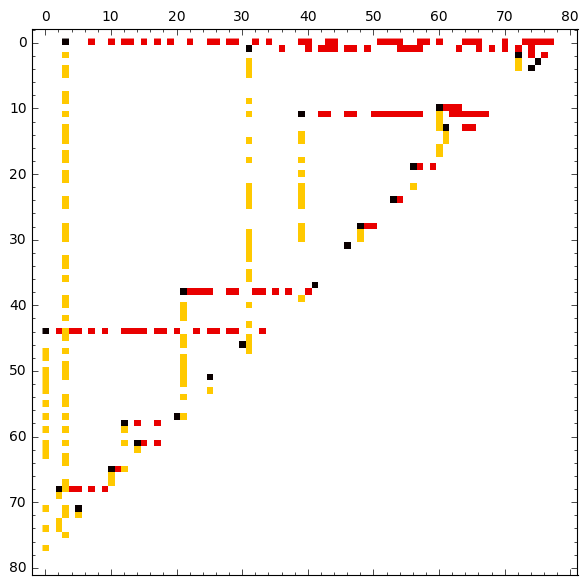
Figure 1: Support of the $\mathcal{L}$ (yellow), $\mathcal{R}$ (black) and $\mathcal{U}$ (red) matrices of the Bruhat generator for a $80\times 80$ left triangular matrix of quasiseparable order $5$.

As the supports of $\mathcal{L}$ and $\mathcal{U}$ are disjoint, the two matrices can be shown on the same left triangular matrix. The pivots of $\mathcal{R}$ (black) are the leading coefficients of every non-zero row of $\mathcal{U}$ and non-zero column of $\mathcal{L}$.

Corollary 16.

Any $(r_{L},r_{U})$-quasiseparable matrix of dimension $n\times n$ can be represented by a generator using no more than $2n(r_{L}+r_{U})+n-2(r_{L}^{2}-2r_{U}^{2})$ field elements and $2(r_{L}+r_{U})$ indices.

Proof.

This estimate is obtained as the space required for the Bruhat representation of the upper and lower triangular parts of the matrix, with $n$ coefficients for the main diagonal. The $2(r_{L}+r_{U})$ indices correspond to the storge of the pivot positions of the two rank profile matrices. ∎

4.3 The compact Bruhat representation

The scattered structure of the Bruhat generator makes it not amenable to the use of fast matrix arithmetic. We therefore propose here a compact variation on it, called the compact Bruhat, that will be used to derive algorithms taking advantage of fast matrix multiplication. This structured representation relies on the generalized Bruhat decomposition described in Manthey and Helmke (2007), thanks to the connection with the rank profile matrix made in Dumas et al. (2016).

Theorem 17 (Generalized Bruhat decomposition (Manthey and Helmke, 2007; Dumas et al., 2016)).

For any $m\times n$ matrix $\mathsf{A}$ of rank $r$, there exist an $m\times r$ matrix $\mathsf{C}$ in column echelon form, an $r\times n$ matrix $\mathsf{E}$ in row echelon form, and an $r\times r$ permutation matrix $\mathsf{R}$ such that $\mathsf{A}=\mathsf{C}\mathsf{R}\mathsf{E}$.

We will also need an additional structure on the echelon form factors.

Definition 18.

Two non-zero columns of matrix are non-overlapping if one has its leading element below the trailing element of the other.

Definition 19.

A matrix is $s$-overlapping if any sub-set of $s+1$ of its non-zero columns contains at least a pair that are non-overlapping.

The motivation for introducing this structure is that left triangular matrices of quasiseparable order $s$ have a generalized Bruhat decomposition with echelon form factors $\mathsf{C}$ and $\mathsf{E}$ that are $s$-overlapping.

Theorem 20.

For any $n\times n$ left triangular matrix $\mathsf{A}$ of quasiseparable order $s$ and of rank $r$, there is a generalized Bruhat decomposition of the form $\mathsf{A}=\text{Left}(\mathsf{C}\mathsf{R}\mathsf{E})$ where $\mathsf{C}$ and $\mathsf{E}^{T}$ are $s$-overlapping.

Proof.

Let $(\mathcal{L},\mathcal{R},\mathcal{U})$ be a Bruhat generator for $\mathsf{A}$. The matrix $\mathcal{L}$ is $s$-overlapping: otherwise, there would be a subset $S$ of $s+1$ of columns such that no pair of them is non-overlapping. Let $((i_{1},j_{1}),\dots,(i_{s+1},j_{s+1}))$ be the coordinates of their leading elements sorted by increasing row index : $i_{1}<i_{2}<\dots<i_{s+1}$. Since $\mathcal{L}$ is left triangular, $j_{s+1}\leq n-i_{s+1}$. The trailing elements of every other column of $S$ must be below row $i_{s+1}$, hence, $j_{k}\leq n-i_{s+1}$ for all $k\leq s$ since $\mathcal{L}$ is left triangular. Consequently the $i_{s+1}\times(n-i_{s+1})$ leading submatrix of $\mathcal{L}$ contains $s+1$ pivots, a contradiction. The same reasonning applies to show that $\mathsf{E}^{T}$ is $s$-overlapping. Consider the permutation matrix $\mathcal{Q}$ such that $\mathcal{L}\mathcal{Q}=\begin{bmatrix}\mathsf{C}&\mathsf{0}_{m\times(n-r)}\end{bmatrix}$ is in column echelon form. Similarly let $\mathcal{P}$ be the permutation matrix such that $\mathcal{P}\mathcal{U}=\begin{bmatrix}\mathsf{E}\\ \mathsf{0}_{(m-r)\times n}\end{bmatrix}$, and remark that $\mathsf{R}=\begin{bmatrix}\mathsf{I}_{r}&\mathsf{0}\end{bmatrix}\mathcal{Q}^{T}\mathcal{R}^{T}\mathcal{P}^{T}\begin{bmatrix}\mathsf{I}_{r}\\ \mathsf{0}\end{bmatrix}$ is a permutation matrix and verifies $\mathsf{A}=\text{Left}(\mathsf{C}\mathsf{R}\mathsf{E})$. ∎

The $s$-overlapping shape of the echelon form factors in the generalized Bruhat decomposition allow to further compress it as follows.

Proposition 21.

Any $s$-overlapping $m\times r$ matrix $\mathsf{A}$ can be written $\mathsf{A}=(\mathsf{D}+\mathsf{S}\mathsf{T})\mathsf{P}$ where $\mathsf{P}$ is a permutation matrix, $\mathsf{T}\in\{0,1\}^{r\times r}$ has at most one non zero element per row and $\mathsf{D}=\text{Diag}(\mathsf{D}_{1},\dots,\mathsf{D}_{t})$, $\mathsf{S}=\left[\begin{smallmatrix}\mathsf{0}\\ \mathsf{S}_{2}&\mathsf{0}\\ &\ddots&\ddots\\ &&\mathsf{S}_{t}\end{smallmatrix}\right]$ where each $\mathsf{D}_{i}$ and $\mathsf{S}_{i}$ is $k_{i}\times s$, except $\mathsf{D}_{t}$ and $\mathsf{S}_{t}$ having possibly fewer columns than $s$ and $\sum_{i=1}^{t}k_{i}=n$.

Intuitively, the permutation $\mathsf{P}^{T}$ sorts the columns of $\mathsf{A}$ in increasing order of their leading row index. Cutting the columns in slices of dimension $s$ makes $\mathsf{A}\mathsf{P}^{T}$ block lower triangular. The block diagonal is $\mathsf{D}$, and the remaining part can be folded into a block sub-diagonal matrix $\mathsf{S}$ thanks to the $s$-overlapping property.

Algorithm 3 Compress-to-Block-Bidiagonal

1:$\mathsf{A}$: an $s$-overlapping matrix

2:$\mathsf{D},\mathsf{S},\mathsf{T},\mathsf{P}$: such that $\mathsf{A}=(\mathsf{D}+\mathsf{S}\mathsf{T})\mathsf{P}$ as in Proposition 21.

3:$\mathsf{P}\leftarrow$ a permutation sorting the columns of $\mathsf{A}$ by increasing row position of their leading coefficient.

4:$\mathsf{C}\leftarrow\mathsf{A}\mathsf{P}\left[\begin{smallmatrix}\mathsf{I}_{r}\\ \mathsf{0}\end{smallmatrix}\right]$ where $r$ is the number of non-zero columns in $\mathsf{A}$

5:Split $\mathsf{C}$ in column slices of width $s$. $\triangleright$ $\mathsf{C}=\left[\begin{smallmatrix}\mathsf{C}_{11}&\\ \mathsf{C}_{21}&\mathsf{C}_{22}\\ \vdots&\vdots&\ddots\\ \mathsf{C}_{t1}&\mathsf{C}_{t2}&\dots&\mathsf{C}_{tt}\end{smallmatrix}\right]$ where $\mathsf{C}_{ii}$ is $k_{i}\times s$ $\forall i<t$.

6:$\mathsf{D}\leftarrow\text{Diag}(\mathsf{C}_{11},\dots,\mathsf{C}_{tt})$

7: $\mathsf{C}\leftarrow\mathsf{C}-\mathsf{D}=\left[\begin{smallmatrix}\mathsf{0}\\ \mathsf{C}_{21}\\ \vdots&\ddots&\ddots\\ \mathsf{C}_{t1}&\dots&\mathsf{C}_{t,t-1}&\mathsf{0}\end{smallmatrix}\right]$

8:$\mathsf{T}\leftarrow\mathsf{I}_{n}$

9:for $i=3\dots t$ do

10:     for each non zero column $j$ of $\left[\begin{smallmatrix}\mathsf{C}_{i,i-2}\\ \dots\\ \mathsf{C}_{t,i-2}\end{smallmatrix}\right]$ do

11:          Let $k$ be a zero column of $\left[\begin{smallmatrix}\mathsf{C}_{i,i-1}\\ \dots\\ \mathsf{C}_{t,i-1}\end{smallmatrix}\right]$

12:          Move column $j$ in $\left[\begin{smallmatrix}\mathsf{C}_{i,i-2}\\ \vdots\\ \mathsf{C}_{t,i-2}\end{smallmatrix}\right]$ to column $k$ in $\left[\begin{smallmatrix}\mathsf{C}_{i,i-1}\\ \vdots\\ \mathsf{C}_{t,i-1}\end{smallmatrix}\right]$.

13:         $\mathsf{T}\leftarrow(\mathsf{I}_{n}+\mathsf{\Delta}^{(k,j)}-\mathsf{\Delta}^{(k,k)})\times\mathsf{T}$

14:     end for

15:end for

16:$\mathsf{S}\leftarrow\mathsf{C}=\left[\begin{smallmatrix}\mathsf{0}&\\ \mathsf{C}_{21}&\mathsf{0}\\ &\ddots&\ddots\\ &&\mathsf{C}_{t,t-1}&\mathsf{0}\end{smallmatrix}\right]$

17:return $(\mathsf{D},\mathsf{S},\mathsf{T},\mathsf{P})$

Algorithm 3 is a constructive proof of Proposition 21, computing a compact representation of any $s$-overlapping matrix.

Proof.

Since $\mathsf{A}$ is $s$-overlapping, there exists a permutation $\mathsf{P}$ such that $\mathsf{C}=\mathsf{A}\mathsf{P}$ is block lower triangular, with blocks of column dimension $s$ except possibly the last one of column dimension $\leq s$. Note that for every $i$, the dimensions of the blocks $\mathsf{S}_{i}$ and $\mathsf{D}_{i}$ are that of the block $\mathsf{C}_{ii}$: $k_{i}\times s$. We then prove that there always exists a zero column to pick at step 11. In the first row of $\begin{bmatrix}\mathsf{C}_{i1}&\dots&\mathsf{C}_{ii}\end{bmatrix}$, there is a non zero element located in the block $\mathsf{C}_{ii}$. As any non-zero column of $\begin{bmatrix}\mathsf{C}_{i1}&\dots&\mathsf{C}_{i,i-1}\end{bmatrix}$ has a leading coefficient in $\mathsf{A}$ at a row index stricly lower than $i$, there can not be more than $s-1$ of them. These $s-1$ columns of $\begin{bmatrix}\mathsf{C}_{i1}&\dots&\mathsf{C}_{i,i-1}\end{bmatrix}$ can all be gathered in the block $\mathsf{C}_{i,i-1}$ of column dimension $s$.

There only remains to show that $\mathsf{S}\mathsf{T}$ is the matrix $\mathsf{C}$ of step 7. For every pair of indices $(j,k)$ selected in loop 9, right multiplication by $(\mathsf{I}_{n}+\mathsf{\Delta}^{(k,j)}-\mathsf{\Delta}^{(k,k)})$ adds up column $k$ to column $j$ and zeroes out column $k$. On matrix $\mathsf{S}$, this has the effect of reverting each operation done at step 12 in the reverse order of the loop 9. ∎

Proposition 22.

If an $s$-overlapping matrix $\mathsf{A}$ is in column echelon form, then, the structured representation $(\mathsf{D},\mathsf{S},\mathsf{T},\mathsf{P})$ is such that $\mathsf{P}=\mathsf{I}_{r}$ and $k_{i}\geq s\ \forall i<t$.

Proof.

The leading elements of each column are already sorted in a column echelon form, hence $\mathsf{P}=\mathsf{I}_{r}$. Then, each block $\mathsf{C}_{ii}$ contains $s$ pivots, hence $k_{i}\geq s$. ∎

We can now define the compact Bruhat representation.

Definition 23.

The compact Bruhat representation of an $n\times n$ $s$-quasiseparable left triangular matrix $\mathsf{A}$ is given by the tuples $(\mathsf{D}^{\mathsf{C}_{\mathsf{A}}},\mathsf{S}^{\mathsf{C}_{\mathsf{A}}},\mathsf{T}^{\mathsf{C}_{\mathsf{A}}})$, $(\mathsf{D}^{\mathsf{E}_{\mathsf{A}}},\mathsf{S}^{\mathsf{E}_{\mathsf{A}}},\mathsf{T}^{\mathsf{E}_{\mathsf{A}}})$ where $\mathsf{D}^{\mathsf{C}_{\mathsf{A}}},\mathsf{S}^{\mathsf{C}_{\mathsf{A}}},(\mathsf{D}^{\mathsf{E}_{\mathsf{A}}})^{T}$ and $(\mathsf{S}^{\mathsf{E}_{\mathsf{A}}})^{T}$ are $n\times r$ block diagonal, with blocks of column dimension $s$, and $\mathsf{T}^{\mathsf{C}_{\mathsf{A}}}$ and $(\mathsf{T}^{\mathsf{E}_{\mathsf{A}}})^{T}$ are lower triangular $\{0,1\}$-matrices with $r$ coefficients equals to $1$ placed on distinct rows, and a permutation matrix $\mathsf{R}^{\mathsf{A}}$ such that

$$\left\{\begin{array}[]{lll}\mathsf{C}^{\mathsf{A}}&=&\mathsf{D}^{\mathsf{C}_{\mathsf{A}}}+\mathsf{S}^{\mathsf{C}_{\mathsf{A}}}\mathsf{T}^{\mathsf{C}_{\mathsf{A}}},\\ \mathsf{E}^{\mathsf{A}}&=&\mathsf{D}^{\mathsf{E}_{\mathsf{A}}}+\mathsf{T}^{\mathsf{E}_{\mathsf{A}}}\mathsf{S}^{\mathsf{E}_{\mathsf{A}}}\\ \end{array}\right.$$

and $\mathsf{A}=\text{Left}(\mathsf{C}^{\mathsf{A}}\mathsf{R}^{\mathsf{A}}\mathsf{E}^{\mathsf{A}})$ is a generalized Bruhat decomposition of $\mathsf{A}$.

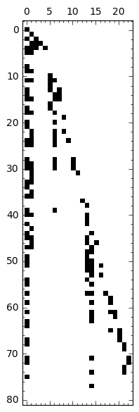
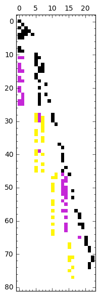
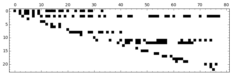
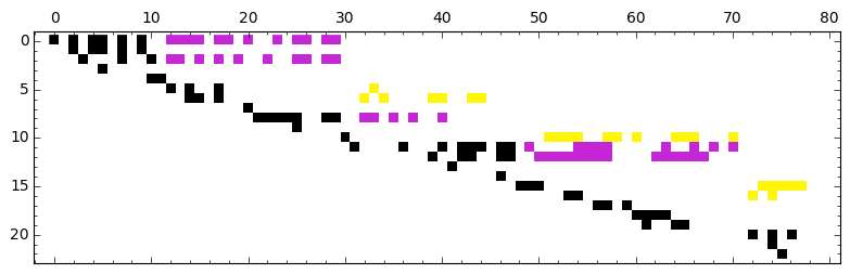
Figure 2: Support of the matrices $\mathsf{C}=\mathcal{L}\mathcal{Q}$ (left), $\mathsf{E}=\mathcal{P}\mathcal{U}$ (top right) of the $s$-overlapping CRE decomposition of Theorem 20 applied to the matrix of Figure 1. The Compression to the block bi-diagonal structure of the corresponding compact Bruhat generator is shown in the central and bottom right matrices. There, $\mathsf{D}$ is in black and $\mathsf{S}$ in magenta and yellow; those rows and columns moved at step 12 of Algorithm 3 are in yellow.

5 Computing with RRR representations

In this section, we will keep considering that the RRR representation is based on any rank revealing factorization (RR), which could originate from various matrix factorizations: PLUQ, CUP, PLE, QR, SVD, etc. We will assume that there exists an algorithm RRF computing such a rank revealing factorization. For instance, PLUQ, CUP, PLE decomposition algorithms can be used to compute such a factorization in time $T_{\texttt{RRF}}(m,n,r)=O(mnr^{\omega-2})$ on an $m\times n$ matrix of rank $r$ (Jeannerod et al., 2013).

5.1 Construction of the generator

The construction of the RRR representation simply consists in computing rank revealing factorizations of all off-diagonal submatrices in a binary splitting of the main diagonal. Let $T_{\texttt{RRR}}(n,s)$ denote the cost of the computation of the binary tree generator for an $n\times n$ matrix of order of quasiseparability $s$. It satisfies the recurrence relation $T_{\texttt{RRR}}(n,s)=2T_{\texttt{RRF}}(n,n,s)+2T_{\texttt{RRR}}(n/2,s)$ which solves in $T_{\texttt{RRR}}(n,s)=O(s^{\omega-2}n^{2})$.

5.2 Matrix-vector product

In the RRR representation, the application of a vector to the quasiseparable matrix takes the same amount of field operations as the number of coefficients used for its representation. This yields a cost of $O(n(r_{L}\log\frac{n}{r_{L}}+r_{U}\log\frac{n}{r_{U}}))=O(sn\log\frac{n}{s})$ field operations.

5.3 Auxiliary algorithms

In the following, we present a set of routines that will be used to build multiplication and inversion algorithms for RRR representations. Algorithm 4 expands a matrix from an RRR representation to a dense representation.

Algorithm 4 RRRExpand: expands an RRR representation into a dense representation

1:$\mathsf{A}$, an $n\times n$ $s$-quasiseparable matrix in an RRR representation,

2:$\mathsf{B}\leftarrow\mathsf{A}$ in a dense representation.

3:if $n\leq s$ then return $\mathsf{B}\leftarrow\mathsf{A}$

4:end if

5:$\mathsf{B}_{11}\leftarrow\texttt{RRRExpand}(\mathsf{A}_{11})$

6:$\mathsf{B}_{22}\leftarrow\texttt{RRRExpand}(\mathsf{A}_{22})$

7:$\mathsf{B}_{12}\leftarrow\mathsf{L}^{\mathsf{A}}_{12}\mathsf{R}^{\mathsf{A}}_{12}$

8:$\mathsf{B}_{21}\leftarrow\mathsf{L}^{\mathsf{A}}_{21}\mathsf{R}^{\mathsf{A}}_{21}$

9:return $\mathsf{B}\leftarrow\begin{bmatrix}\mathsf{B}_{11}&\mathsf{B}_{12}\\ \mathsf{B}_{21}&\mathsf{B}_{22}\end{bmatrix}$

The recurring relation $T_{\texttt{RRRExpand}}(n,s)=2T_{\texttt{RRRExpand}}(n/2,s)+O(n^{2}s^{\omega-2})$ for $n>s$ yields directly

$$T_{\texttt{RRRExpand}}(n,s)=O(n^{2}s^{\omega-2}).$$

Algorithm 5 multiplies two rank revealing factorizations and outputs the result in a rank revealing factorization. As $\mathsf{L}^{\mathsf{A}}$ and $\mathsf{L}^{\mathsf{X}}$ have full column rank, so is their product. Hence the $\mathsf{L}^{\mathsf{C}}\mathsf{R}^{\mathsf{C}}$ is a rank revealing factorization of the product.

Algorithm 5 RRxRR: multiplies two matrices stored as rank revealing factorization

1:$\mathsf{A}$, an $m\times k$ matrix of rank $\leq s$ in an RR representation $\mathsf{L}^{\mathsf{A}}\times\mathsf{R}^{\mathsf{A}}$,

2:$\mathsf{B}$, an $k\times n$ matrix of rank $\leq t$ in an RR representation $\mathsf{L}^{\mathsf{B}}\times\mathsf{R}^{\mathsf{B}}$,

3:$\mathsf{C}\leftarrow\mathsf{A}\times\mathsf{B}$ in an RR representation $\mathsf{L}^{\mathsf{C}}\times\mathsf{R}^{\mathsf{C}}$.

4:$\mathsf{X}\leftarrow\mathsf{R}^{\mathsf{A}}\mathsf{L}^{\mathsf{B}}$

5:$(\mathsf{L}^{\mathsf{X}},\mathsf{R}^{\mathsf{X}})\leftarrow\texttt{RRF}(\mathsf{X})$ $\triangleright$ Computes the RR factorization $\mathsf{X}=\mathsf{L}^{\mathsf{X}}\times\mathsf{R}^{\mathsf{X}}$

6:$\mathsf{L}^{\mathsf{C}}\leftarrow\mathsf{L}^{\mathsf{A}}\mathsf{L}^{\mathsf{X}}$

7:$\mathsf{R}^{\mathsf{C}}\leftarrow\mathsf{R}^{\mathsf{X}}\mathsf{R}^{\mathsf{B}}$

The resulting cost (assuming $s\leq t$ without loss of generality) is

$$T_{\texttt{RRxRR}}(m,k,n,s,t)=O(s^{\omega-2}tk)+T_{\texttt{RRF}}(s,t)+O(r_{\mathsf{X}}^{\omega-2}(ms+nt)).$$

With $n=\Theta(m)=\Theta(k)$, this is $T_{\texttt{RRxRR}}(n,s,t)=O((s+t)^{\omega-1}n).$

Algorithm 6 adds two rank revealing factorizations. It first stacks together the left sides and the right sides of the rank revealing factorizations of the two terms. The resulting factorization may not reveal the rank as the inner dimension may be larger. Therefore, a rank revealing factorization of each factor is first computed, before invoquing RRxRR to obtain an RR representation of their product.

Algorithm 6 RR+RR: adds two matrices stored as rank revealing factorization

1:$\mathsf{A}$, an $m\times n$ matrix of rank $\leq s$ in an RR representation $\mathsf{L}^{\mathsf{A}}\times\mathsf{R}^{\mathsf{A}}$

2:$\mathsf{B}$, an $m\times n$ matrix of rank $\leq t$ in an RR representation $\mathsf{L}^{\mathsf{B}}\times\mathsf{R}^{\mathsf{B}}$

3:$\mathsf{D}\leftarrow\mathsf{A}+\mathsf{B}$ in an RR representation $\mathsf{L}^{\mathsf{D}}\times\mathsf{R}^{\mathsf{D}}$.

4:$\mathsf{X}\leftarrow\begin{bmatrix}\mathsf{L}^{\mathsf{A}}&\mathsf{L}^{\mathsf{B}}\end{bmatrix}$; $\mathsf{Y}\leftarrow\begin{bmatrix}\mathsf{R}^{\mathsf{A}}\\ \mathsf{R}^{\mathsf{B}}\end{bmatrix}$

5:$(\mathsf{L}^{\mathsf{X}},\mathsf{R}^{\mathsf{X}})\leftarrow\texttt{RRF}(\mathsf{X})$ $\triangleright$ $\mathsf{X}=\mathsf{L}^{\mathsf{X}}\times\mathsf{R}^{\mathsf{X}}$, $r_{\mathsf{X}}=\text{rank}(\mathsf{X})$; $\mathsf{L}^{\mathsf{X}}$ is $m\times r_{\mathsf{X}}$ and $\mathsf{R}^{\mathsf{X}}$ is $r_{\mathsf{X}}\times n$

6:$(\mathsf{L}^{\mathsf{Y}},\mathsf{R}^{\mathsf{Y}})\leftarrow\texttt{RRF}(\mathsf{Y})$ $\triangleright$ $\mathsf{Y}=\mathsf{L}^{\mathsf{Y}}\times\mathsf{R}^{\mathsf{Y}}$, $r_{\mathsf{Y}}=\text{rank}(\mathsf{Y})$; $\mathsf{L}^{\mathsf{Y}}$ is $m\times r_{\mathsf{Y}}$ and $\mathsf{R}^{\mathsf{Y}}$ is $r_{\mathsf{Y}}\times n$

7:$\mathsf{D}\leftarrow\texttt{RRxRR}(\mathsf{X},\mathsf{Y})$ $\triangleright$ Computes an RR representation of the product $\mathsf{D}=\mathsf{X}\mathsf{Y}$

Assuming $n=\Theta(m)$, the time complexity is

$$T_{\texttt{RR+RR}}(n,s,t)=2T_{\texttt{RRF}}(n,s+t)+O((s+t)^{\omega-1}n)=O((s+t)^{\omega-1}n).$$

Algorithm 7 adds a quasiseparable matrix in RRR representation with a matrix in RR representation.

Algorithm 7 RRR+RR: adds a quasiseparable matrix in RRR representation and a rank revealing factorization

1:$\mathsf{A}$, an $n\times n$ $s$-quasiseparable matrix in an RRR representation

2:$\mathsf{B}$, an $n\times n$ matrix of rank $\leq t$ in an RR representation $\mathsf{L}^{\mathsf{B}}\times\mathsf{R}^{\mathsf{B}}$

3:$\mathsf{C}\leftarrow\mathsf{A}+\mathsf{B}$ in an RRR representation.

4:if $n\leq s+t$ then

5:     return $\mathsf{C}\leftarrow$ $\texttt{RRRExpand}(\mathsf{A})+\mathsf{L}^{\mathsf{B}}\times\mathsf{R}^{\mathsf{B}}$

6:end if

7:Split the matrices as $\begin{bmatrix}\mathsf{C}_{11}&\mathsf{C}_{12}\\ \mathsf{C}_{21}&\mathsf{C}_{22}\end{bmatrix}\leftarrow\begin{bmatrix}\mathsf{A}_{11}&\mathsf{A}_{12}\\ \mathsf{A}_{21}&\mathsf{A}_{22}\end{bmatrix}+\begin{bmatrix}\mathsf{B}_{11}&\mathsf{B}_{12}\\ \mathsf{B}_{21}&\mathsf{B}_{22}\end{bmatrix}$.

8:$\mathsf{C}_{11}\leftarrow\texttt{RRR+RR}(\mathsf{A}_{11},\mathsf{B}_{11})$ $\triangleright$ $\mathsf{C}_{11}\leftarrow\mathsf{A}_{11}+\mathsf{B}_{11}$

9:$\mathsf{C}_{22}\leftarrow\texttt{RRR+RR}(\mathsf{A}_{22},\mathsf{B}_{22})$ $\triangleright$ $\mathsf{C}_{11}\leftarrow\mathsf{A}_{22}+\mathsf{B}_{22}$

10:$\mathsf{C}_{12}\leftarrow\texttt{RR+RR}(\mathsf{A}_{12},\mathsf{B}_{12})$ $\triangleright$ $\mathsf{C}_{12}\leftarrow\mathsf{A}_{12}+\mathsf{B}_{12}$

11:$\mathsf{C}_{21}\leftarrow\texttt{RR+RR}(\mathsf{A}_{21},\mathsf{B}_{21})$ $\triangleright$ $\mathsf{C}_{21}\leftarrow\mathsf{A}_{21}+\mathsf{B}_{21}$

12:return $\mathsf{C}\leftarrow\begin{bmatrix}\mathsf{C}_{11}&\mathsf{C}_{12}\\ \mathsf{C}_{21}&\mathsf{C}_{22}\end{bmatrix}$

The time complexity satisfies the recurring relation

$$\left\{\begin{array}[]{llll}T_{\texttt{RRR+RR}}(n,s,t)&=&2T_{\texttt{RRR+RR}}(n/2,s,t)+2T_{\texttt{RR+RR}}(n/2,s,t)&\text{ for }n>s+t\\ &=&2T_{\texttt{RRR+RR}}(n/2,s,t)+O(n(s+t)^{\omega-1})\\ T_{\texttt{RRR+RR}}(n,s,t)&=&T_{\texttt{RRRExpand}}(s+t,s)+O((s+t)^{2}t^{\omega-2})&\text{ for }n\leq s+t\end{array}\right.$$

which solves in

$$T_{\texttt{RRR+RR}}(n,s,t) = O((s+t)^{\omega-1}n\log\frac{n}{s+t}+\frac{n}{s+t}(s+t)^{2}(s^{\omega-2}+t^{\omega-2})$$

$$= O((s+t)^{\omega-1}n\log\frac{n}{s+t}).$$

5.4 Quasiseparable times tall and skinny

Algorithm 8 RRRxTS: multiplies a quasiseparable matrix in RRR representation with a tall and skinny matrix

1:$\mathsf{A}$, an $n\times n$ $s$-quasiseparable matrix in RRR representation

2:$\mathsf{B}$, an $n\times t$ matrix

3:$\mathsf{C}\leftarrow\mathsf{A}\mathsf{B}$

4:if $n\leq s+t$ then

5:     return $\mathsf{C}\leftarrow\texttt{RRRExpand}(\mathsf{A})\times\mathsf{B}$

6:end if

7:Split the matrices as $\begin{bmatrix}\mathsf{C}_{1}\\ \mathsf{C}_{2}\end{bmatrix}\leftarrow\begin{bmatrix}\mathsf{A}_{11}&\mathsf{A}_{12}\\ \mathsf{A}_{21}&\mathsf{A}_{22}\end{bmatrix}\begin{bmatrix}\mathsf{B}_{1}\\ \mathsf{B}_{2}\end{bmatrix}$.

8:$\mathsf{C}_{1}\leftarrow\texttt{RRRxTS}(\mathsf{A}_{11},\mathsf{B}_{1})$ $\triangleright$ $\mathsf{C}_{1}\leftarrow\mathsf{A}_{11}\mathsf{B}_{1}$

9:$\mathsf{C}_{2}\leftarrow\texttt{RRRxTS}(\mathsf{A}_{22},\mathsf{B}_{2})$ $\triangleright$ $\mathsf{C}_{2}\leftarrow\mathsf{A}_{22}\mathsf{B}_{2}$

10:$\mathsf{X}\leftarrow\mathsf{R}^{\mathsf{A}}_{12}\mathsf{B_{2}}$

11:$\mathsf{C}_{1}\leftarrow\mathsf{C_{1}}+\mathsf{L}^{\mathsf{A}}_{12}\mathsf{X}$ $\triangleright$ $\mathsf{C_{1}}\leftarrow\mathsf{C_{1}}+\mathsf{A}_{12}\mathsf{B}_{2}$

12:$\mathsf{Y}\leftarrow\mathsf{R}^{\mathsf{A}}_{21}\mathsf{B_{1}}$

13:$\mathsf{C}_{2}\leftarrow\mathsf{C_{2}}+\mathsf{L}^{\mathsf{A}}_{21}\mathsf{Y}$ $\triangleright$ $\mathsf{C_{2}}\leftarrow\mathsf{C_{2}}+\mathsf{A}_{21}\mathsf{B}_{1}$

14:return $\mathsf{C}\leftarrow\begin{bmatrix}\mathsf{C}_{1}\\ \mathsf{C}_{2}\end{bmatrix}$

Algorithm 8 multiplies an $s$-quasiseparable matrix of dimension $n\times n$ in RRR representation by a tall and skinny matrix: an $n\times t$ rectangular dense matrix with $t\leq n$.

Let $T_{\texttt{RRRxTS}}(n,s,t)$ denote its cost. The recurring relation

$$\left\{\begin{array}[]{llll}T_{\texttt{RRRxTS}}(n,s,t)&=&2T_{\texttt{RRRxTS}}(n/2,s,t)+O(n\max(s,t)\min(s,t)^{\omega-2})&\text{ for }n>s+t\\ T_{\texttt{RRRxTS}}(n,s,t)&=&T_{\texttt{RRRExpand}}(s+t,s)+O((s+t)^{2}t^{\omega-2})&\text{ for }n\leq s+t\end{array}\right.$$

yields

$$T_{\texttt{RRRxTS}}(n,s,t) = O((s+t)^{\omega-1}n\log\frac{n}{s+t}+\frac{n}{s+t}(s+t)^{2}(s^{\omega-2}+t^{\omega-2})$$

$$= O((s+t)^{\omega-1}n\log\frac{n}{s+t}).$$

From this algorithm, follows Algorithm 9, computing the product of an $s$-quasiseparable matrix in RRR representation by a rank revealing factorization. Similarly as for Algorithm 5, $\mathsf{R}^{\mathsf{X}}$ and $\mathsf{R}^{\mathsf{B}}$ have full row rank, so has their product, which ensures that the factors $\mathsf{L}^{\mathsf{D}},\mathsf{R}^{\mathsf{D}}$ form a rank revealing factorization of the result.

Algorithm 9 RRRxRR: multiplies a quasiseparable matrix in RRR representation with a rank revealing factorization

1:$\mathsf{A}$, an $n\times n$ $s$-quasiseparable matrix in RRR representation

2:$\mathsf{B}$, an $n\times m$ matrix of rank $\leq t$ in an RR representation $\mathsf{L}^{\mathsf{B}}\times\mathsf{R}^{\mathsf{B}}$

3:$\mathsf{D}\leftarrow\mathsf{A}\mathsf{B}$ in a rank revealing factorization $\mathsf{L}^{\mathsf{D}}\times\mathsf{R}^{\mathsf{D}}$

4:$\mathsf{X}\leftarrow\texttt{RRRxTS}(\mathsf{A},\mathsf{L}^{\mathsf{B}})$ $\triangleright$ $\mathsf{X}\leftarrow\mathsf{A}\mathsf{L}^{\mathsf{B}}$

5:$(\mathsf{L}^{\mathsf{X}},\mathsf{R}^{\mathsf{X}})\leftarrow\texttt{RRF}(\mathsf{X})$ $\triangleright$ Computes the RR factorization $\mathsf{X}=\mathsf{L}^{\mathsf{X}}\times\mathsf{R}^{\mathsf{X}}$

6:$\mathsf{L}^{\mathsf{D}}\leftarrow\mathsf{L}^{\mathsf{X}}$

7:$\mathsf{R}^{\mathsf{D}}\leftarrow\mathsf{R}^{\mathsf{X}}\mathsf{R}^{\mathsf{B}}$

Its time complexity is

$$T_{\texttt{RRRxRR}}(n,s,t)=T_{\texttt{RRRxTS}}(n,s,t)+T_{\texttt{RRF}}(n,t)+O(nt^{\omega-1})=O((s+t)^{\omega-1}n\log\frac{n}{s+t})$$

5.5 Quasiseparable times Quasiseparable

The product of an $s$-quasiseparable matrix by a $t$-quasiseparable matrix is an $(s+t)$-quasiseparable matrix (Eidelman and Gohberg, 1999). Algorithm 10, calling Algorithms 5, 6, 7 and 8, shows how to perform such a multiplication with the RRR representations.

Algorithm 10 RRRxRRR

1:$\mathsf{A}$, an $n\times n$ $s$-quasiseparable matrix in an RRR representation,

2:$\mathsf{B}$, an $n\times n$ $t$-quasiseparable matrix in an RRR representation,

3:$\mathsf{C}\leftarrow\mathsf{A}\times\mathsf{B}$ in an RRR representation.

4:if $n\leq s+t$ then

5:     return $\mathsf{C}\leftarrow\texttt{RRRExpand}(\mathsf{A})\times\texttt{RRRExpand}(\mathsf{B})$

6:end if

7:Split the matrices as $\begin{bmatrix}\mathsf{C}_{11}&\mathsf{C}_{12}\\ \mathsf{C}_{21}&\mathsf{C}_{22}\end{bmatrix}\leftarrow\begin{bmatrix}\mathsf{A}_{11}&\mathsf{A}_{12}\\ \mathsf{A}_{21}&\mathsf{A}_{22}\end{bmatrix}\begin{bmatrix}\mathsf{B}_{11}&\mathsf{B}_{12}\\ \mathsf{B}_{21}&\mathsf{B}_{22}\end{bmatrix}$.

8:$\mathsf{C}_{11}\leftarrow$ RRRxRRR $(\mathsf{A}_{11},\mathsf{B}_{11})$ $\triangleright$ $\mathsf{C}_{11}\leftarrow\mathsf{A}_{11}\mathsf{B}_{11}$

9:$\mathsf{C}_{22}\leftarrow$ RRRxRRR $(\mathsf{A}_{22},\mathsf{B}_{22})$ $\triangleright$ $\mathsf{C}_{22}\leftarrow\mathsf{A}_{22}\mathsf{B}_{22}$

10:$\mathsf{X}\leftarrow$ RRxRR $(\mathsf{A}_{12},\mathsf{B}_{21})$ $\triangleright$ $\mathsf{X}\leftarrow\mathsf{A}_{12}\mathsf{B}_{21}$

11:$\mathsf{Y}\leftarrow$ RRxRR $(\mathsf{A}_{21},\mathsf{B}_{12})$ $\triangleright$ $\mathsf{Y}\leftarrow\mathsf{A}_{21}\mathsf{B}_{12}$

12:$\mathsf{C}_{11}\leftarrow$ RRR+RR $(\mathsf{C}_{11},\mathsf{X})$ $\triangleright$ $\mathsf{C}_{11}\leftarrow\mathsf{C}_{11}+\mathsf{X}$

13:$\mathsf{C}_{22}\leftarrow$ RRR+RR $(\mathsf{C}_{22},\mathsf{Y})$ $\triangleright$ $\mathsf{C}_{22}\leftarrow\mathsf{C}_{22}+\mathsf{Y}$

14:$\mathsf{L}^{\mathsf{X}}\leftarrow\texttt{RRRxTS}(\mathsf{A}_{11},\mathsf{L}^{\mathsf{B}}_{12})$; $\mathsf{R}^{\mathsf{X}}\leftarrow\mathsf{R}^{\mathsf{B}}_{12}$ $\triangleright$ $\mathsf{X}\leftarrow\mathsf{A}_{11}\mathsf{B}_{12}$ in RR representation

15:$\mathsf{L}^{\mathsf{Y}}\leftarrow\mathsf{L}^{\mathsf{A}}_{12}$; $\mathsf{R}^{\mathsf{Y}}\leftarrow\texttt{TSxRRR}(\mathsf{R}^{\mathsf{A}}_{12},\mathsf{B}_{22})$ $\triangleright$ $\mathsf{Y}\leftarrow\mathsf{A}_{12}\mathsf{B}_{22}$ in RR representation revealing factorization

16:$\mathsf{C}_{12}\leftarrow\texttt{RR+RR}(\mathsf{X},\mathsf{Y})$ $\triangleright$ $\mathsf{C}_{12}\leftarrow\mathsf{X}+\mathsf{Y}$

17:$\mathsf{L}^{\mathsf{X}}\leftarrow\texttt{RRRxTS}(\mathsf{A}_{11},\mathsf{L}^{\mathsf{B}}_{21})$; $\mathsf{R}^{\mathsf{X}}\leftarrow\mathsf{R}^{\mathsf{B}}_{21}$ $\triangleright$ $\mathsf{X}\leftarrow\mathsf{A}_{11}\mathsf{B}_{21}$ in RR representation

18:$\mathsf{L}^{\mathsf{Y}}\leftarrow\mathsf{L}^{\mathsf{A}}_{21}$; $\mathsf{R}^{\mathsf{Y}}\leftarrow\texttt{TSxRRR}(\mathsf{R}^{\mathsf{A}}_{21},\mathsf{B}_{22})$ $\triangleright$ $\mathsf{Y}\leftarrow\mathsf{A}_{21}\mathsf{B}_{22}$ in RR representation

19:$\mathsf{C}_{21}\leftarrow\texttt{RR+RR}(\mathsf{X},\mathsf{Y})$ $\triangleright$ $\mathsf{C}_{21}\leftarrow\mathsf{X}+\mathsf{Y}$

20:return $\mathsf{C}\leftarrow\begin{bmatrix}\mathsf{C}_{11}&\mathsf{C}_{12}\\ \mathsf{C}_{21}&\mathsf{C}_{22}\\ \end{bmatrix}$

In steps 12 and 13, a $(s+t)$-quasiseparable matrix is added to a rank revealing factorization of rank $(s+t)$. It should in general result in an RRR representation of an $2(s+t)$-quasiseparable matrix. However, the matrix $\mathsf{C}$ is no more than $(s+t)$-quasiseparable, hence the rank revealing factorization of the result, will have rank only $s+t$. The reductions to RR representation, performed in step 5 of Algorithm 5 and steps 5 and 6 of Algorithm 6, ensure that this factorization will be reduced to this size.

Let $T_{\texttt{RRR$\times$RRR}}(n,s,t)$ denote the time complexity of this algorithm. If $n\leq s+t$, then $T_{\texttt{RRRxRRR}}(n,s,t)=T_{\texttt{RRRExpand}}(n,s)+T_{\texttt{RRRExpand}}(n,t)+O(n^{\omega})=O((s+t)^{\omega}).$ Now consider the case $n>s+t$.

$$T_{\texttt{RRRxRRR}}(n,s,t) = 2T_{\texttt{RRRxRRR}}(n/2,s,t)+2T_{\texttt{RRxRR}}(n/2,s,t)+2T_{\texttt{RRRxTS}}(n/2,s,t)$$

$$+2T_{\texttt{RRR+RR}}(n/2,s+t,s+t)+2T_{\texttt{RR+RR}}(n/2,s+t,s+t)$$

$$= 2T_{\texttt{RRRxRRR}}(n/2,s,t)+O((s+t)^{\omega-1}n\log\frac{n}{s+t})$$

Consequently, $T_{\texttt{RRRxRRR}}(n,s,t)=O((s+t)^{\omega-1}n\log^{2}\frac{n}{s+t})$.

5.6 Computing the inverse in RRR representation

We consider the case, as in (Eidelman and Gohberg, 1999, § 6), where the matrix to be inverted has generic rank profile, i.e. all of its leading principal minors are non-vanishing. Under this assumption, Strassen’s divide and conquer algorithm (Strassen, 1969) reduces the computation of the inverse to matrix multiplication. More precisely, the inverse is recursively computed using the following block $2\times 2$ formula:

$$\begin{bmatrix}\mathsf{A}_{11}&\mathsf{A}_{12}\\ \mathsf{A}_{21}&\mathsf{A}_{22}\\ \end{bmatrix}^{-1}=\begin{bmatrix}\mathsf{A}_{11}^{-1}+\mathsf{A}_{11}^{-1}\mathsf{A}_{12}\mathsf{D}^{-1}\mathsf{A}_{21}\mathsf{A}_{11}^{-1}&-\mathsf{A}_{11}^{-1}\mathsf{A}_{12}\mathsf{D}^{-1}\\ -\mathsf{D}^{-1}\mathsf{A}_{21}\mathsf{A}_{11}^{-1}&\mathsf{D}^{-1}\\ \end{bmatrix},$$

where $\mathsf{D}=\mathsf{A}_{22}-\mathsf{A}_{21}\mathsf{A}_{11}^{-1}\mathsf{A}_{12}$.

This formula leads to a recursive algorithm that we adapt to the case of quasiseparable matrices in RRR representation in algorithm 11.

Algorithm 11 RRRinvert: compute the inverse in RRR representation

1:$\mathsf{A}$, an $n\times n$ $s$-quasiseparable strongly regular matrix in RRR representation,

2:$\mathsf{X}=\mathsf{A}^{-1}$, $s$-quasiseparable in RRR representation.

3:if $n\leq s$ then

4:     $\mathsf{Y}\leftarrow\texttt{RRRExpand}(\mathsf{A})$

5:     return $\mathsf{X}\leftarrow\texttt{Invert}(\mathsf{Y})$

6:end if

7:Split the matrix as $\mathsf{A}=\begin{bmatrix}\mathsf{A}_{11}&\mathsf{A}_{12}\\ \mathsf{A}_{21}&\mathsf{A}_{22}\end{bmatrix}$ and $\mathsf{X}=\begin{bmatrix}\mathsf{X}_{11}&\mathsf{X}_{12}\\ \mathsf{X}_{21}&\mathsf{X}_{22}\end{bmatrix}$

8:$\mathsf{Y}_{11}\leftarrow\texttt{RRRinvert}(\mathsf{A}_{11})$ $\triangleright$ $\mathsf{Y}_{11}=\mathsf{A}_{11}^{-1}$

9:$\mathsf{Y}_{12}\leftarrow\texttt{RRRxRR}(\mathsf{Y}_{11},\mathsf{A}_{12})$ $\triangleright$ $\mathsf{Y}_{12}\leftarrow\mathsf{A}_{11}^{-1}\mathsf{A}_{12}$

10:$\mathsf{Y}_{21}\leftarrow\texttt{RRRxRR}(\mathsf{A}_{21},\mathsf{Y}_{11})$ $\triangleright$ $\mathsf{Y}_{21}\leftarrow\mathsf{A}_{21}\mathsf{A}_{11}^{-1}$

11:$\mathsf{Z}\leftarrow-\texttt{RRxRR}(\mathsf{A}_{21}\mathsf{Y}_{12})$ $\triangleright$ $\mathsf{Z}\leftarrow-\mathsf{A}_{21}\mathsf{A}_{11}^{-1}\mathsf{A}_{12}$

12:$\mathsf{D}\leftarrow\texttt{RR+RR}(\mathsf{A}_{22},\mathsf{Z})$ $\triangleright$ $\mathsf{D}\leftarrow\mathsf{A}_{22}-\mathsf{A}_{21}\mathsf{A}_{11}^{-1}\mathsf{A}_{12}$

13:$\mathsf{X}_{22}\leftarrow\texttt{RRRinvert}(\mathsf{D})$ $\triangleright$ $\mathsf{X}_{22}=\mathsf{D}^{-1}$

14:$\mathsf{X}_{21}\leftarrow-\texttt{RRRxRR}(\mathsf{X}_{22},\mathsf{Y}_{21})$ $\triangleright$ $\mathsf{X}_{21}\leftarrow-\mathsf{D}^{-1}\mathsf{A}_{21}\mathsf{A}_{11}^{-1}$

15:$\mathsf{W}\leftarrow-\texttt{RRxRR}(\mathsf{Y}_{12},\mathsf{X}_{21})$ $\triangleright$ $\mathsf{W}\leftarrow\mathsf{A}_{11}^{-1}\mathsf{A}_{12}\mathsf{D}^{-1}\mathsf{A}_{21}\mathsf{A}_{11}^{-1}$

16:$\mathsf{X}_{12}\leftarrow-\texttt{RRRxRR}(\mathsf{Y}_{12},\mathsf{X}_{22})$ $\triangleright$ $\mathsf{X}_{12}\leftarrow-\mathsf{A}_{11}^{-1}\mathsf{A}_{12}\mathsf{D}^{-1}$

17:$\mathsf{X}_{11}\leftarrow\texttt{RRR+RR}(\mathsf{Y}_{11},\mathsf{W})$ $\triangleright$ $\mathsf{X}_{11}\leftarrow\mathsf{A}_{11}^{-1}+\mathsf{A}_{11}^{-1}\mathsf{A}_{12}\mathsf{D}^{-1}\mathsf{A}_{21}\mathsf{A}_{11}^{-1}$

18:return $\mathsf{X}=\begin{bmatrix}\mathsf{X}_{11}&\mathsf{X}_{12}\\ \mathsf{X}_{21}&\mathsf{X}_{22}\\ \end{bmatrix}$.

The fact that the inverse matrix $\mathsf{X}$ is itself $s$-quasiseparable, implies that the matrix $\mathsf{D}$ is also $s$-quasiseparable and not $2s$-quasiseparable, as the generic upper bound would say. The compression happens in the RR+RR routine, at step 12. Hence all operations except the recursive calls take $O(s^{\omega-1}n\log\frac{n}{s})$. The overall complexity of Algorithm 11 is therefore $T_{\texttt{RRRInverse}}(n,s)=O(s^{\omega-1}n\log^{2}\frac{n}{s})$.

6 Computing with a Compact Bruhat representation

6.1 Construction of the generator

We first propose in Algorithm 12 an evolution of Algorithm 2 to compute the factors of the Bruhat generator (without compression) for a left triangular matrix.

Algorithm 12 LT-Bruhat

1:$\mathsf{A}$: an $n\times n$ matrix

2:$(\mathcal{L},\mathcal{R},\mathcal{U})$: a Bruhat generator for the left triangular part of $\mathsf{A}$

3:if $n=1$ then return $([0],[0],[0])$

4:Split $\mathsf{A}=\begin{bmatrix}\mathsf{A_{1}}&\mathsf{A_{2}}\\ \mathsf{A_{3}}\end{bmatrix}$ where $\mathsf{A_{3}}$ is $\lfloor\frac{n}{2}\rfloor\times\lfloor\frac{n}{2}\rfloor$

5:Decompose $\mathsf{A_{1}}=\mathsf{P_{1}}\begin{bmatrix}\mathsf{L_{1}}\\ \mathsf{M_{1}}\end{bmatrix}\begin{bmatrix}\mathsf{U_{1}}&\mathsf{V_{1}}\end{bmatrix}\mathsf{Q_{1}}$

6:$\mathsf{R_{1}}\leftarrow\mathsf{P_{1}}\begin{bmatrix}\mathsf{I_{r_{1}}}\\ &\mathsf{0}\end{bmatrix}\mathsf{Q_{1}}$ where $r_{1}=\text{rank}(\mathsf{A_{1}})$.

7:$\begin{bmatrix}\mathsf{B_{1}}\\ \mathsf{B_{2}}\end{bmatrix}\leftarrow\mathsf{P_{1}}^{T}\mathsf{A_{2}}$

8:$\begin{bmatrix}\mathsf{C_{1}}&\mathsf{C_{2}}\end{bmatrix}\leftarrow\mathsf{A_{3}}\mathsf{Q_{1}}^{T}$

9:Here $A=\left[\begin{array}[]{cc|c}\mathsf{L_{1}}\backslash\mathsf{U_{1}}&\mathsf{V_{1}}&\mathsf{B_{1}}\\ \mathsf{M_{1}}&\mathsf{0}&\mathsf{B_{2}}\\ \hline\cr\mathsf{C_{1}}&\mathsf{C_{2}}&\\ \end{array}\right]$.

10:$\mathsf{D}\leftarrow\mathsf{L_{1}}^{-1}\mathsf{B_{1}}$

11:$\mathsf{E}\leftarrow\mathsf{C_{1}}\mathsf{U_{1}}^{-1}$

12:$\mathsf{F}\leftarrow\mathsf{B_{2}}-\mathsf{M_{1}}\mathsf{D}$

13:$\mathsf{G}\leftarrow\mathsf{C_{2}}-\mathsf{E}\mathsf{V_{1}}$

14:Here $\mathsf{A}=\left[\begin{array}[]{cc|c}\mathsf{L_{1}}\backslash\mathsf{U_{1}}&\mathsf{V_{1}}&\mathsf{D}\\ \mathsf{M_{1}}&\mathsf{0}&\mathsf{F}\\ \hline\cr\mathsf{E}&\mathsf{G}&\\ \end{array}\right]$.

15:$\mathsf{H}\leftarrow\mathsf{P_{1}}\begin{bmatrix}\mathsf{0}_{r_{1}\times\frac{n}{2}}\\ \mathsf{F}\end{bmatrix}$

16:$\mathsf{I}\leftarrow\begin{bmatrix}\mathsf{0}_{r_{1}\times\frac{n}{2}}&\mathsf{G}\end{bmatrix}\mathsf{Q_{1}}$

17: $(\mathcal{L}_{2},\mathcal{R}_{2},\mathcal{U}_{2})\leftarrow\texttt{LT-Bruhat}(\mathsf{H})$

18: $(\mathcal{L}_{3},\mathcal{R}_{3},\mathcal{U}_{3})\leftarrow\texttt{LT-Bruhat}(\mathsf{I})$

19:$\mathcal{L}\leftarrow\begin{bmatrix}\mathsf{P}_{1}\begin{bmatrix}\mathsf{L}_{1}&\mathsf{0}\\ \mathsf{M}_{1}&\mathsf{0}\\ \end{bmatrix}\mathsf{Q}_{1}&\mathsf{0}\\ \text{Left}(\begin{bmatrix}\mathsf{E}&\mathsf{0}\end{bmatrix}\mathsf{Q}_{1})&\mathsf{0}\end{bmatrix}+\begin{bmatrix}\mathsf{0}&\mathcal{L}_{2}\\ \mathcal{L}_{3}\end{bmatrix}$

20:$\mathcal{U}\leftarrow\begin{bmatrix}\mathsf{P}_{1}\begin{bmatrix}\mathsf{U}_{1}&V_{1}\\ \mathsf{0}&\mathsf{0}\end{bmatrix}\mathsf{Q}_{1}&\text{Left}(\mathsf{P}_{1}\begin{bmatrix}\mathsf{D}\\ \mathsf{0}\end{bmatrix})\\ \mathsf{0}&\mathsf{0}\end{bmatrix}+\begin{bmatrix}\mathsf{0}&\mathcal{U}_{2}\\ \mathcal{U}_{3}\end{bmatrix}$

21:$\mathcal{R}\leftarrow\begin{bmatrix}\mathcal{R}_{1}&\mathcal{R}_{2}\\ \mathcal{R}_{3}\end{bmatrix}$

22:return $(\mathcal{L},\mathcal{R},\mathcal{U})$

Theorem 24.

For any $n\times n$ matrix $\mathsf{A}$ with a left triangular part of quasiseparable order $s$, Algorithm 12 computes the Bruhat generator of the left triangular part of $\mathsf{A}$ in $O(s^{\omega-2}n^{2})$ field operations.

Proof.

The correctness of $\mathcal{R}$ is proven in Theorem 10. We will prove by induction the correctness of $\mathcal{U}$, noting that the correctness of $\mathcal{L}$ works similarly.

Let $\mathsf{H}=\mathsf{P}_{2}\mathsf{L}_{2}\mathsf{U}_{2}\mathsf{Q}_{2}$ and $\mathsf{I}=\mathsf{P}_{3}\mathsf{L}_{3}\mathsf{U}_{3}\mathsf{Q}_{3}$ be PLUQ decompositions of $\mathsf{H}$ and $\mathsf{I}$ revealing their rank profile matrices. Assume that Algorithm LT-Bruhat is correct in the two recursive calls 17 and 18, that is

$$\begin{array}[]{ll}\mathcal{U}_{2}=\text{Left}(\mathsf{P}_{2}\begin{bmatrix}\mathsf{U}_{2}\\ \mathsf{0}\end{bmatrix}\mathsf{Q}_{2}),&\mathcal{U}_{3}=\text{Left}(\mathsf{P}_{3}\begin{bmatrix}\mathsf{U}_{3}\\ \mathsf{0}\end{bmatrix}\mathsf{Q}_{3}),\\ \mathcal{L}_{2}=\text{Left}(\mathsf{P}_{2}\begin{bmatrix}\mathsf{L}_{2}&\mathsf{0}\end{bmatrix}\mathsf{Q}_{2}),&\mathcal{L}_{3}=\text{Left}(\mathsf{P}_{3}\begin{bmatrix}\mathsf{L}_{3}&\mathsf{0}\end{bmatrix}\mathsf{Q}_{3}).\\ \end{array}$$

At step 9, we have

$$\begin{bmatrix}\mathsf{A}_{1}&\mathsf{A}_{2}\\ \mathsf{A}_{3}&*\end{bmatrix}=\begin{bmatrix}\mathsf{P}_{1}\\ &\mathsf{I}_{\frac{n}{2}}\end{bmatrix}\left[\begin{array}[]{cc|c}\mathsf{L}_{1}&&\\ \mathsf{M}_{1}&\mathsf{I}_{\frac{n}{2}-r_{1}}\\ \hline\cr\mathsf{E}&\mathsf{0}&\mathsf{I}_{\frac{n}{2}}\end{array}\right]\left[\begin{array}[]{cc|c}\mathsf{U}_{1}&\mathsf{V}_{1}&\mathsf{D}\\ &\mathsf{0}&\mathsf{F}\\ \hline\cr&\mathsf{G}&\end{array}\right]\begin{bmatrix}\mathsf{Q}_{1}\\ &\mathsf{I}_{\frac{n}{2}}\end{bmatrix}$$

As the first $r_{1}$ rows of $\mathsf{P}_{1}^{T}\mathsf{H}$ are zeros, there exists $\mathsf{\bar{P}}_{2}$ a permutation matrix and $\mathsf{\bar{L}}_{2}$, a lower triangular matrix, such that $\mathsf{P}_{1}^{T}\mathsf{P}_{2}\mathsf{L}_{2}=\begin{bmatrix}\mathsf{0}_{r_{1}\times\frac{n}{2}}\\ \mathsf{\bar{P}}_{2}\mathsf{\bar{L}}_{2}\end{bmatrix}$. Similarly, there exsist $\mathsf{\bar{Q}}_{3}$, a permutation matrix and $\mathsf{\bar{U}}_{3}$, an upper triangular matrix, such that $\mathsf{U}_{3}\mathsf{Q}_{3}\mathsf{Q}_{1}^{T}=\begin{bmatrix}\mathsf{0}_{\frac{n}{2}\times r_{1}}&\mathsf{\bar{U}}_{3}\mathsf{\bar{Q}}_{3}\end{bmatrix}$. Hence

$$\begin{bmatrix}\mathsf{A}_{1}&\mathsf{A}_{2}\\ \mathsf{A}_{3}&*\end{bmatrix}=\begin{bmatrix}\mathsf{P}_{1}\\ &\mathsf{P}_{3}\end{bmatrix}\left[\begin{array}[]{cc|c}\mathsf{L}_{1}&&\\ \mathsf{M}_{1}&\mathsf{\bar{P}}_{2}\mathsf{\bar{L}}_{2}\\ \hline\cr\mathsf{P}_{3}^{T}\mathsf{E}&\mathsf{0}&\mathsf{L}_{3}\end{array}\right]\left[\begin{array}[]{cc|c}\mathsf{U}_{1}&\mathsf{V}_{1}&\mathsf{D}\mathsf{Q}_{2}^{T}\\ &\mathsf{0}&\mathsf{U_{2}}\\ &\mathsf{\bar{U}}_{3}\mathsf{\bar{Q}}_{3}\end{array}\right]\begin{bmatrix}\mathsf{Q}_{1}\\ &\mathsf{Q}_{2}\end{bmatrix}\\$$

Setting $\mathsf{N}_{1}=\mathsf{\bar{P}}_{2}^{T}\mathsf{M}_{1}$ and $\mathsf{W}_{1}=\mathsf{V}_{1}\mathsf{\bar{Q}}_{3}^{T}$, we have

$$\begin{bmatrix}\mathsf{A}_{1}&\mathsf{A}_{2}\\ \mathsf{A}_{3}&*\end{bmatrix}=\begin{bmatrix}\mathsf{P}_{1}\begin{bmatrix}\mathsf{I}_{r_{1}}\\ &\mathsf{\bar{P}}_{2}\end{bmatrix}\\ &\mathsf{P}_{3}\end{bmatrix}\left[\begin{array}[]{ccc}\mathsf{L}_{1}\\ \mathsf{N}_{1}&\mathsf{\bar{L}}_{2}\\ \hline\cr\mathsf{E}&\mathsf{0}&\mathsf{\mathsf{L_{3}}}\end{array}\right]\left[\begin{array}[]{cc|c}\mathsf{U}_{1}&\mathsf{W}_{1}&\mathsf{D}\mathsf{Q}_{2}^{T}\\ &\mathsf{0}&\mathsf{U_{2}}\\ &\mathsf{\bar{U}}_{3}\end{array}\right]\begin{bmatrix}\begin{bmatrix}\mathsf{I}_{r_{1}}\\ &\mathsf{\bar{Q}}_{3}\end{bmatrix}\mathsf{Q}_{1}\\ &\mathsf{Q}_{2}\end{bmatrix}.$$

A PLUQ of $\left[\begin{smallmatrix}\mathsf{A}_{1}&\mathsf{A}_{2}\\ \mathsf{A}_{3}\end{smallmatrix}\right]$ revealing its rank profile matrix is then obtained from this decomposition by a row block cylic-shift on the second factor and a column block cyclic shift on the third factor as in (Dumas et al., 2013, Algorithm 1).

Finally,

$$\mathsf{P}\begin{bmatrix}\mathsf{U}\\ 0\end{bmatrix}\mathsf{Q} = \begin{bmatrix}\mathsf{P}_{1}\\ &\mathsf{I}_{\frac{n}{2}}\end{bmatrix}\begin{bmatrix}\mathsf{U}_{1}&\mathsf{V}_{1}&\mathsf{D}\\ &\mathsf{0}&\mathsf{\bar{P}}_{2}\mathsf{U}_{2}\mathsf{Q}_{2}\\ &\mathsf{P}_{3}\mathsf{\bar{U}}_{3}\mathsf{\bar{Q}}_{3}\\ \mathsf{0}&\mathsf{0}&\mathsf{0}\end{bmatrix}\begin{bmatrix}\mathsf{Q}_{1}\\ &\mathsf{I}_{\frac{n}{2}}\end{bmatrix}$$

$$= \begin{bmatrix}\mathsf{P}_{1}\begin{bmatrix}\mathsf{U}_{1}&\mathsf{V}_{1}\\ \mathsf{0}&\mathsf{0}\end{bmatrix}\mathsf{Q}_{1}&\mathsf{P}_{1}\begin{bmatrix}\mathsf{D}\\ \mathsf{0}\end{bmatrix}\\ \mathsf{0}&\mathsf{0}\ \end{bmatrix}+\begin{bmatrix}&\mathsf{P}_{2}\begin{bmatrix}\mathsf{U}_{2}\\ \mathsf{0}\end{bmatrix}\mathsf{Q}_{2}\\ \mathsf{P}_{3}\begin{bmatrix}\mathsf{U}_{3}\\ \mathsf{0}\end{bmatrix}\mathsf{Q}_{3}\end{bmatrix}.$$

Hence $\text{Left}(\mathsf{P}\mathsf{U}\mathsf{Q})=\begin{bmatrix}\mathsf{P}_{1}\begin{bmatrix}\mathsf{U}_{1}&\mathsf{V}_{1}\\ \mathsf{0}&\mathsf{0}\end{bmatrix}\mathsf{Q}_{1}&\text{Left}(\mathsf{P}_{1}\begin{bmatrix}\mathsf{D}\\ \mathsf{0}\end{bmatrix})\\ \mathsf{0}&\mathsf{0}\\ \end{bmatrix}+\begin{bmatrix}&\mathcal{U}_{2}\\ \mathcal{U}_{3}\end{bmatrix}.$

The complexity analysis is exactly that of Theorem 10. ∎

The computation of a compact Bruhat generator, as shown in Algorithm 13, is then directly obtained by combining Algorithm 12 with Algorithm 3.

Algorithm 13 Compact Bruhat generator

1:$\mathsf{A}$: an $n\times n$ left triangular matrix of quasiseparable order $s$

2: $(\mathsf{D}^{{\mathsf{C}_{\mathsf{L}}}},\mathsf{S}^{{\mathsf{C}_{\mathsf{L}}}},\mathsf{T}^{{\mathsf{C}_{\mathsf{L}}}}),\mathsf{R}_{\mathsf{L}},(\mathsf{D}^{{\mathsf{E}_{\mathsf{L}}}},\mathsf{S}^{{\mathsf{E}_{\mathsf{L}}}},\mathsf{T}^{{\mathsf{E}_{\mathsf{L}}}})$ : a Compact Bruhat generator for $\mathsf{L}=\text{Left}(\mathsf{J}_{n}\mathsf{A})$

3: $(\mathsf{D}^{{\mathsf{C}_{\mathsf{U}}}},\mathsf{S}^{{\mathsf{C}_{\mathsf{U}}}},\mathsf{T}^{{\mathsf{C}_{\mathsf{U}}}}),\mathsf{R}_{\mathsf{U}},(\mathsf{D}^{{\mathsf{E}_{\mathsf{U}}}},\mathsf{S}^{{\mathsf{E}_{\mathsf{U}}}},\mathsf{T}^{{\mathsf{E}_{\mathsf{U}}}})$ : a Compact Bruhat generator for $\mathsf{U}=\text{Left}(\mathsf{A}\mathsf{J}_{n})$

4:$\mathsf{L}\leftarrow\text{Left}(\mathsf{J}_{n}\mathsf{A})$

5:$\mathsf{U}\leftarrow\text{Left}(\mathsf{A}\mathsf{J}_{n})$

6:$(\mathcal{L}_{\mathsf{L}},\mathcal{R}_{\mathsf{L}},\mathcal{U}_{\mathsf{L}})\leftarrow\texttt{LT-Bruhat}(\mathsf{L})$

7:$(\mathcal{L}_{\mathsf{U}},\mathcal{R}_{\mathsf{U}},\mathcal{U}_{\mathsf{U}})\leftarrow\texttt{LT-Bruhat}(\mathsf{U})$

8:$(\mathsf{D}^{{\mathsf{C}_{\mathsf{L}}}},\mathsf{S}^{{\mathsf{C}_{\mathsf{L}}}},\mathsf{T}^{{\mathsf{C}_{\mathsf{L}}}},\mathsf{P}^{\mathsf{C}_{\mathsf{L}}})\leftarrow\texttt{Compress-to-Block-Bidiagonal}(\mathcal{L}_{\mathsf{L}})$

9:$(\mathsf{D}^{{\mathsf{E}_{\mathsf{L}}}},\mathsf{S}^{{\mathsf{E}_{\mathsf{L}}}},\mathsf{T}^{{\mathsf{E}_{\mathsf{L}}}},\mathsf{P}^{\mathsf{E}_{\mathsf{L}}})\leftarrow(\texttt{Compress-to-Block-Bidiagonal}(\mathcal{U}_{\mathsf{L}}^{T}))^{T}$

10:$\mathsf{R}_{\mathsf{L}}\leftarrow\begin{bmatrix}\mathsf{I}_{r}&\mathsf{0}\end{bmatrix}\mathsf{P}^{\mathsf{C}_{\mathsf{L}}}\mathcal{R}_{\mathsf{L}}^{T}\mathsf{P}^{\mathsf{E}_{\mathsf{L}}}\begin{bmatrix}\mathsf{I}_{r}\\ \mathsf{0}\end{bmatrix}$

11:$\mathsf{R}_{\mathsf{U}}\leftarrow\begin{bmatrix}\mathsf{I}_{r}&\mathsf{0}\end{bmatrix}\mathsf{P}^{\mathsf{C}_{\mathsf{U}}}\mathcal{R}_{\mathsf{U}}^{T}\mathsf{P}^{\mathsf{E}_{\mathsf{U}}}\begin{bmatrix}\mathsf{I}_{r}\\ \mathsf{0}\end{bmatrix}$

6.2 Multiplication by a tall and skinny matrix

We consider the multiplication of an $s$-quasiseparable matrix in Compact Bruhat representation by an $n\times t$ dense rectangular matrix ($t\leq s$), and show that is can be performed in $O(st^{\omega-2}n)=O(s^{\omega-1}n)$ field operations.

The Compact Bruhat representation stores a representation of two left triangular matrices, corresponding to the upper and lower triangular parts of the matrix. Hence it suffices to show how to multiply an $s$-quasiseparable left triangular matrix in Compact Bruhat representation with a tall and skinny matrix.

Using the Definition 23, this means computing

$$\mathsf{C}=\text{Left}(\mathsf{C}^{\mathsf{A}}\mathsf{R}^{\mathsf{A}}\mathsf{E}^{\mathsf{A}})\mathsf{B}$$

where $B$ is dense $n\times t$. Without the Left operator, the target complexity $O(s^{\omega-1}n)$ would be reached by first computing the product $\mathsf{E}^{\mathsf{A}}\mathsf{B}$ and then applying $\mathsf{R}^{\mathsf{A}}$ and $\mathsf{C}^{\mathsf{A}}$ on the left. However because of the Left operator, each row of the result matrix $\mathsf{C}$ involves a distinct partial sum of the product $\mathsf{E}^{\mathsf{A}}\mathsf{B}$:

$$\mathsf{C}_{i,*}=\mathsf{C}^{\mathsf{A}}_{i,*}\mathsf{R}^{\mathsf{A}}\left(\sum_{j=1}^{n-i}\mathsf{E}^{\mathsf{A}}_{*,j}\mathsf{B}_{j,*}\right).$$

We will therefore avoid computing the accumulation in this product, keeping point-wise products available in memory. In order to reach the target complexity, the products of dimension $s$ will be computed with accumulation, keeping the terms of the unevaluated sum available at the level of size $s$ blocks.

Cutting these matrices on a grid of size $s$, let $N=\lceil n/s\rceil$ and $\mathsf{C}=\begin{bmatrix}\mathsf{C}_{1}&\dots&\mathsf{C}_{N}\end{bmatrix}^{T}$, $\mathsf{E}^{\mathsf{A}}=\begin{bmatrix}\mathsf{E}^{\mathsf{A}}_{1}&\dots&\mathsf{E}^{\mathsf{A}}_{N}\end{bmatrix}$, $\mathsf{C}^{\mathsf{A}}=\begin{bmatrix}\mathsf{C}^{\mathsf{A}}_{1}&\dots&\mathsf{C}^{\mathsf{A}}_{N}\end{bmatrix}^{T}$ and $\mathsf{B}=\begin{bmatrix}\mathsf{B}_{1}&\dots&\mathsf{B}_{N}\end{bmatrix}^{T}$. We have

$$\mathsf{C}_{i}=\mathsf{C}^{\mathsf{A}}_{i}\mathsf{R}^{\mathsf{A}}\sum_{j=1}^{N-i}\mathsf{E}^{\mathsf{A}}_{j}\mathsf{B}_{j}+\text{Left}\left(\mathsf{C}^{\mathsf{A}}_{i}\mathsf{R}^{\mathsf{A}}\mathsf{E}^{\mathsf{A}}_{N-i+1}\right)\mathsf{B}_{N-i+1}.$$

Each of these blocks $\mathsf{C}_{i}$ are then computed as shown in Algorithm 14.

Algorithm 14 LeftCBxTS

1:$\mathsf{A}$, an $n\times n$ $s$-quasiseparable left triangular matrix: $\mathsf{A}=\text{Left}(\mathsf{C}^{\mathsf{A}}\mathsf{R}^{\mathsf{A}}\mathsf{E}^{\mathsf{A}})$

2:$\mathsf{B}$, an $n\times t$ matrix

3:$\mathsf{C}\leftarrow\mathsf{A}\mathsf{B}$, an $n\times t$ dense tall and skinny matrix

4:for $j=1\dots N-1$ do

5:     $\mathsf{X}_{j}\leftarrow\mathsf{E}^{\mathsf{A}}_{j}\mathsf{B}_{j}$ $\triangleright$ in a compact representation $\mathsf{X}_{j}=\mathsf{D}_{j}^{\mathsf{X}}+\mathsf{T}^{\mathsf{E}}\mathsf{S}_{j}^{\mathsf{X}}$

6:      $\mathsf{Y}_{j}\leftarrow\mathsf{R}^{\mathsf{A}}\mathsf{X}_{j}$$\triangleright$ expand $\mathsf{D}_{j}^{\mathsf{X}}+\mathsf{T}^{\mathsf{E}}\mathsf{S}_{j}^{\mathsf{X}}$ and apply the permutation $\mathsf{R}^{\mathsf{A}}$

7:end for

8: compute all partial sums of these blocks: $\mathsf{Z}_{i}=\sum_{j=1}^{N-i}\mathsf{Y}_{j}$;

9: apply $\mathsf{C}_{i}^{\mathsf{A}}$ to the left: $\mathsf{V}_{i}=\mathsf{C}^{\mathsf{A}}_{i}\mathsf{Z}_{i}$;

10: add the trailing term, $\mathsf{C}_{i}=\mathsf{V}_{i}+\text{Left}\left(\mathsf{C}_{i}^{\mathsf{A}}\mathsf{R}^{\mathsf{A}}\mathsf{E}^{\mathsf{A}}_{N-i+1})\mathsf{B}_{N-i+1}\right)$.

11:return $\mathsf{C}\leftarrow\begin{bmatrix}\mathsf{C}_{1}\\ \vdots\\ \mathsf{C}_{N}\end{bmatrix}$

In the compact Bruhat representation, the row echelon form $\mathsf{E}^{\mathsf{A}}$ is stored in the form $\mathsf{E}^{\mathsf{A}}=\mathsf{D}^{\mathsf{E}}+\mathsf{T}^{\mathsf{E}}\mathsf{S}^{\mathsf{E}}$ where $\mathsf{D}$ and $\mathsf{S}$ are block diagonal with blocks of dimension $s\times k_{j}$ where $k_{j}\geq s$.

Step 5

reduces to computing $\mathsf{D}_{j}^{\mathsf{X}}=\mathsf{D}_{j}^{\mathsf{E}}\mathsf{B}_{j}$ and $\mathsf{S}_{j}^{\mathsf{X}}=\mathsf{S}_{j}^{\mathsf{E}}\mathsf{B}_{j}$ such that

$$\mathsf{X}_{j}=\mathsf{D}_{j}^{\mathsf{X}}+\mathsf{T}^{\mathsf{E}}\mathsf{S}_{j}^{\mathsf{X}}.$$ (7)

Each of these products requires $O(k_{j}st^{\omega-2})$ field operations, hence Step 5 costs $O(nst^{\omega-2})$ field operations. After Step 5, the matrix $\mathsf{X}$ is stored in a compact representation, given by equation (7), requiring only $O(nt)$ space.

Step 6

does not involve any field operation as the multiplication on the left by $\mathsf{T}^{\mathsf{E}}$ and the final sum act on matrices of non-overlapping support. The overall amount of data being copied is linear in the number of non-zero elements: $O(nt)$.

Step 8

can be achieved by computing the prefix sum of the $\mathsf{Y}_{i}$’s: $\mathsf{Z}_{1}=\mathsf{Y}_{1}$ and $\mathsf{Z}_{i}=\mathsf{Z}_{i-1}+\mathsf{Y}_{i}$. Each step involves $O(st)$ additions (the number of non zero elements in $\mathsf{Y}_{i}$), hence Step 8 costs $O(nt)$ field operations.

Step 9

is a sequence of $N$ products of an $s\times r$ matrix $\mathsf{C}^{\mathsf{A}}_{i}=\mathsf{D}_{i}^{\mathsf{C}}+\mathsf{S}_{i}^{\mathsf{C}}\mathsf{T}^{\mathsf{C}}$ by an $r\times r$ matrix $\mathsf{Z}_{i}$. As both $\mathsf{D}_{i}^{\mathsf{C}}$ and $\mathsf{S}_{i}^{\mathsf{C}}$ have only $s$ continuous non-zero columns, each of these product costs $O(s^{2}t^{\omega-2})$ and the overall cost is $O(nst^{\omega-2})$.

Step 10

is achieved by computing the $s\times s$ factor $\text{Left}(\mathsf{C}_{i}^{\mathsf{A}}\mathsf{R}^{\mathsf{A}}\mathsf{E}^{\mathsf{A}}_{N-i+1})$ explicitly in $O(s^{\omega})$, and then applying it to $\mathsf{B}_{N-i+1}$ in $O(s^{2}t^{\omega-2})$.

Overall the cost of algorithm 14 is $O(nts^{\omega-2})$ field operations.

Corollary 25.

An $s$-quasiseparable matrix in Compact Bruhat representation can be multiplied

1. by a vector in time $O(ns)$

2. by a dense $n\times m$ matrix in time $O(s^{\omega-2}nm)$.

3. by a another $s$-quasiseparable matrix matrix in time $O(s^{\omega-2}n^{2})$.

Proof.

1. Specializing this LeftCBxTS algorithm with $t=1$ yields an algorithm for multiplying by vector in time $O(ns)$.

2. Splitting the dense matrix in $\lceil\frac{m}{s}\rceil$ slices and applying LeftCBxTS on each of them takes $O(s^{\omega-1}n\lceil\frac{m}{s}\rceil)=O(s^{\omega-2}nm)$.

3. Expanding one of the two matrices into a dense representation and multiplying it to the other one takes $O(s^{\omega-2}n^{2})$.

∎

The last item in the corollary improves over the complexity of multiplying two dense matrices in $O(n^{\omega})$. However, the result being itself a $2s$-quasiseparable matrix, it could be presented in a Compact Bruhat representation. Hence the target cost for this operation is far below: $O(s^{\omega-1}n)$ since both input and output have size $O(sn)$. Applying similar techniques as in Algorithm 14, we could only produce the output as two terms of the form $\text{Left}(\mathsf{L}\mathsf{R})$ where $\mathsf{L}$ and $\mathsf{R}^{T}$ are $n\times(\text{rank}(\mathsf{A})+\text{rank}(\mathsf{B}))$ in time $O(s^{\omega-1}n)$, but we were unable to perform the compression to a Compact Bruhat representation within this target complexity for the moment.

References

- Bini and Pan (1994) Bini, D., Pan, V., 1994. Polynomial and Matrix Computations, Volume 1: Fundamental Algorithms. Birkhauser, Boston.
-
Boito et al. (2016)
Boito, P., Eidelman, Y., Gemignani, L., 2016. Implicit QR for companion-like
pencils. Math. of Computation 85 (300), 1753–1774.
URL http://www.ams.org/mcom/2016-85-300/S0025-5718-2015-03020-8/ -
Bostan et al. (2008)
Bostan, A., Jeannerod, C.-P., Schost, E., Nov. 2008. Solving structured linear
systems with large displacement rank. Theoretical Computer Science
407 (1–3), 155–181.
URL http://www.sciencedirect.com/science/article/pii/S0304397508003940 -
Bruhat (1956)
Bruhat, F., 1956. Sur les représentations induites des groupes de Lie.
Bulletin de la Société Mathématique de France 84, 97–205.
URL http://eudml.org/doc/86911 -
Carrier et al. (1988)
Carrier, J., Greengard, L., Rokhlin, V., Jul. 1988. A Fast Adaptive
Multipole Algorithm for Particle Simulations. SIAM Journal on
Scientific and Statistical Computing 9 (4), 669–686.
URL http://epubs.siam.org/doi/abs/10.1137/0909044 -
Chan (1987)
Chan, T. F., Apr. 1987. Rank revealing QR factorizations. Linear Algebra and
its Applications 88, 67–82.
URL http://www.sciencedirect.com/science/article/pii/0024379587901030 -
Chandrasekaran et al. (2005)
Chandrasekaran, S., Dewilde, P., Gu, M., Pals, T., Sun, X., van der Veen, A.,
White, D., Jan. 2005. Some Fast Algorithms for Sequentially
Semiseparable Representations. SIAM Journal on Matrix Analysis and
Applications 27 (2), 341–364.
URL http://epubs.siam.org/doi/abs/10.1137/S0895479802405884 -
Chandrasekaran et al. (2006)
Chandrasekaran, S., Gu, M., Pals, T., Jan. 2006. A Fast ULV Decomposition
Solver for Hierarchically Semiseparable Representations. SIAM Journal
on Matrix Analysis and Applications 28 (3), 603–622.
URL http://epubs.siam.org/doi/abs/10.1137/S0895479803436652 -
Chandrasekaran and Ipsen (1994)
Chandrasekaran, S., Ipsen, I., Apr. 1994. On Rank-Revealing
Factorisations. SIAM Journal on Matrix Analysis and Applications 15 (2),
592–622.
URL http://epubs.siam.org/doi/abs/10.1137/S0895479891223781 -
Delvaux and Van Barel (2007)
Delvaux, S., Van Barel, M., Nov. 2007. A Givens-Weight Representation for
Rank Structured Matrices. SIAM J. on Matrix Analysis and Applications
29 (4), 1147–1170.
URL http://epubs.siam.org/doi/abs/10.1137/060654967 - Dumas et al. (2013) Dumas, J.-G., Pernet, C., Sultan, Z., 2013. Simultaneous computation of the row and column rank profiles. In: Kauers, M. (Ed.), Proc. ISSAC’13. ACM Press, pp. 181–188.
-