WKB Approximation for a Deformed Schrodinger-like Equation and its Applications to Quasinormal Modes of Black Holes and Quantum Cosmology

Abstract

In this paper, we use the WKB approximation method to approximately solve a deformed Schrodinger-like differential equation: $\left[-\hbar^{2}\partial_{\xi}^{2}g^{2}\left(-i\hbar\alpha\partial_{\xi}\right)-p^{2}\left(\xi\right)\right]\psi\left(\xi\right)=0$, which are frequently dealt with in various effective models of quantum gravity, where the parameter $\alpha$ characterizes effects of quantum gravity. For an arbitrary function $g\left(x\right)$ satisfying several properties proposed in the paper, we find the WKB solutions, the WKB connection formulas through a turning point, the deformed Bohr–Sommerfeld quantization rule, and the deformed tunneling rate formula through a potential barrier. Several examples of applying the WKB approximation to the deformed quantum mechanics are investigated. In particular, we calculate the bound states of the Pöschl-Teller potential and estimate the effects of quantum gravity on the quasinormal modes of a Schwarzschild black hole. Moreover, the area quantum of the black hole is considered via Bohr’s correspondence principle. Finally, the WKB solutions of the deformed Wheeler–DeWitt equation for a closed Friedmann universe with a scalar field are obtained, and the effects of quantum gravity on the probability of sufficient inflation is discussed in the context of the tunneling proposal.

I Introduction

The WKB approximation, named after Wentzel, Kramers, and Brillouin, is a method for obtaining an approximate solution to a one-dimensional Schrodinger-like differential equation:

$$\left[-\hbar^{2}\partial_{\xi}^{2}-p^{2}\left(\xi\right)\right]\psi\left(\xi\right)=0,$$ (1)

where the real function $p^{2}\left(\xi\right)$ can be either positively or negatively valued. The WKB approximation has a wide range of applications. Its principal applications are in calculating bound-state energies and tunneling rates through potential barriers.

On the other hand, the construction of a quantum theory for gravity has posed one of the most challenging problems of the theoretical physics. Although there are various proposals for quantum gravity, a comprehensive theory is not available yet. Rather than considering a full quantum theory of gravity, we can instead study effective theories of quantum gravity. In various effective models of quantum gravity, one always deals with a deformed Schrodinger-like equation:

$$\left[P^{2}\left(-i\hbar\partial_{\xi}\right)-p^{2}\left(\xi\right)\right]\psi\left(\xi\right)=0,$$ (2)

where $P\left(x\right)=xg\left(\alpha x\right)$. The properties of the function $g\left(x\right)$ will be discussed in section II. Note that the parameter $\alpha$ characterizes effects of quantum gravity. For example, the deformed Schrodinger-like equation $\left(\ref{eq:DeformedEq}\right)$ could appear in two effective models, namely the Generalized Uncertainty Principle (GUP) and the modified dispersion relation (MDR). We will briefly show that how it appears in these two models in section III.

The WKB approximation in deformed space and its applications have been considered in effective models of quantum gravity. For example, in the framework of GUP, the WKB wave functions were obtained in IN-Fityo:2005lwa . Moreover, the deformed Bohr–Sommerfeld quantization rule and tunneling rate formula were used to calculate bound states of Harmonic oscillators and Hydrogen atoms IN-Fityo:2005lwa , $\alpha$-decay IN-Blado:2015ada ; IN-Guo:2016btf , quantum cosmogenesis IN-Blado:2015ada , the volume of a phase cell IN-Tao:2012fp , and electron emissions IN-Guo:2016btf , for some specific function $g\left(x\right)$. In the context of both GUP and MDR, the deformed Bohr–Sommerfeld quantization rule was used to compute the number of quantum states to find the entanglement entropy of black holes in the brick wall model IN-Wang:2015bwa ; IN-Eune:2010kx ; IN-Wang:2015zpa . In IN-Tao:2012fp ; IN-Guo:2016btf , we found the WKB connection formulas and proved the deformed Bohr–Sommerfeld quantization rule and tunneling rate formula for the $g\left(x\right)=\sqrt{1+x^{2}}$ case. In this paper, we will consider the case with an arbitrary function $g\left(x\right)$, for which the WKB connection formulas, Bohr–Sommerfeld quantization rule and tunneling rate formula are obtained.

The organization of this paper is as follows. In section II, the deformed Schrodinger-like differential equation $\left(\ref{eq:DeformedEq}\right)$ are first approximately solved by the WKB method. After the asymptotic behavior of exact solutions of eqn. $\left(\ref{eq:DeformedEq}\right)$ around turning points are found, we obtain the WKB connection formulas through a turning point by matching these two solutions in the overlap regions. Accordingly, the Bohr–Sommerfeld quantization rule and tunneling rate formula are also given. In section III, the formulas obtained in section II are used to investigate several examples, namely harmonic oscillators, the Schwinger effect, the Pöschl-Teller potential, and quantum cosmology. Section IV is devoted to our discussion and conclusion. In the appendix, we plot the contours used to compute the asymptotic behavior in the $g\left(x\right)=\frac{\tan\left(x\right)}{x}$ case.

II WKB Method

We now apply the WKB method to approximately solve the deformed Schrodinger-like differential equation $\left(\ref{eq:DeformedEq}\right)$. In what follows, we choose that $\arg p\left(\xi\right)=0$ for $p^{2}\left(\xi\right)>0$ and $\arg p\left(\xi\right)=\frac{\pi}{2}$ for $p^{2}\left(\xi\right)<0$. Moreover, we could rewrite $P\left(x\right)$ in terms of a new function $g\left(x\right)$ as

$$P\left(x\right)=xg\left(\alpha x\right)\text{.}$$ (3)

To study the WKB solutions of eqn. $\left(\ref{eq:DeformedEq}\right)$ and the connection formulas through a turning point, we shall impose the following conditions on the function $g\left(x\right)$:

• In the complex plane, $g\left(z\right)$ is assumed to be analytic except for possible poles. We assume that $g\left(0\right)=1$.

• For a positive real number $a>0$, each of the equations

  $$sg\left(-ias\right)=e^{i\pi k/2}\text{, with }k=0\text{, }1\text{, }2\text{, }3,$$ (4)

  possess only one regular solution $\lambda_{k}\left(a\right)$, which is regular as $a\rightarrow 0$ and becomes

  $$\lambda_{k}\left(0\right)=e^{i\pi k/2}\text{,}$$ (5)

  and the possible runaway solutions $\eta_{k}^{\left(i\right)}\left(a\right)$, which becomes

  $$\eta_{k}^{\left(i\right)}\left(a\right)\sim\frac{\eta_{k}^{\left(i\right)}}{a},$$ (6)

  when $a\ll 1$. We also assume that for small enough value of $a$, there exists a $c_{1}>0$ such that for all possible $i$ and $k$,

  $$\frac{c_{1}}{a}<\left|\eta_{k}^{\left(i\right)}\left(a\right)\right|\text{.}$$ (7)

  If there is no runaway solution, we simply set $c_{1}=\infty$.

• Finally, we assume that there exists a $c_{2}>0$ such that

  $$\left|g^{2}\left(-is\right)-1\right|\leq\frac{1}{2}\text{ for }\left|s\right|\leq c_{2}.$$ (8)

For example, $g\left(x\right)=1\pm x^{2}$ satisfies the above conditions with $\exists 0<c_{1}<1$ and $0<c_{2}\leq 1/\sqrt{2}$. The function $g\left(x\right)=\frac{\tan x}{x}$ also satisfies the above conditions with $\exists 0<c_{1}<\pi$ and $0<c_{2}\leq\arctan\left(3/2\right)$.

II.1 WKB Solutions

To find an approximate solution via the WKB method, we could make the change of variable

$$\psi\left(\xi\right)=e^{\frac{iS\left(\xi\right)}{\hbar}}$$ (9)

for some function $S\left(\xi\right)$, which can be expanded in power series over $\hbar$

$$S\left(\xi\right)=S_{0}\left(\xi\right)+\frac{\hbar}{i}S_{1}\left(\xi\right)+\cdots.$$ (10)

Plugging eqn. $\left(\ref{eq:S}\right)$ into eqn. $\left(\ref{eq:DeformedEq}\right)$ gives

$$P^{2}\left(S_{0}^{\prime}\left(\xi\right)\right) =p^{2}\left(\xi\right),$$

$$\left[P^{2}\left(S_{0}^{\prime}\left(\xi\right)\right)\right]^{\prime}\frac{\hbar}{i}S_{1}\left(\xi\right) =\frac{i\hbar}{2}\left[P^{2}\left(S_{0}^{\prime}\left(\xi\right)\right)\right]^{\prime\prime}S_{0}^{\prime\prime}\left(\xi\right),$$ (11)

where the prime denotes derivative with respect to the argument of the corresponding function. The first equation in eqn. $\left(\ref{eq:sexpand}\right)$ can be solved for $S_{0}^{\prime}\left(\xi\right)$. In particular, when $p^{2}\left(\xi\right)>0$,

$$S_{0}^{\prime}\left(\xi\right)=-i\left|p\left(\xi\right)\right|\lambda_{k}\left(\alpha\left|p\left(\xi\right)\right|\right)\text{, with }k=1\text{ and }3\text{,}$$ (12)

and when $p^{2}\left(\xi\right)<0$,

$$S_{0}^{\prime}\left(\xi\right)=-i\left|p\left(\xi\right)\right|\lambda_{k}\left(\alpha\left|p\left(\xi\right)\right|\right)\text{, with }k=0\text{ and }2\text{,}$$ (13)

where $\lambda_{k}\left(a\right)$ are regular solutions of eqn. $\left(\ref{eq:lamda}\right)$. It is noteworthy that there are other possible solutions, namely

$$S_{0}^{\prime}\left(\xi\right)=-i\left|p\left(\xi\right)\right|\eta_{k}\left(\alpha\left|p\left(\xi\right)\right|\right).$$ (14)

These solutions are called ”runaways” solutions since they do not exist in the limit of $\alpha\rightarrow 0$. In WKB-Simon:1990ic , it was argued that these ”runaways” solutions were not physical and hence should be discarded. A similar argument was also given in the framework of the GUP WKB-Ching:2012fu . Therefore, we will discard the ”runaways” solutions and keep only the solutions $\left(\ref{eq:k=1and3}\right)$ and $\left(\ref{eq:k=0and2}\right)$ in this paper. Solving the second equation in eqn. $\left(\ref{eq:sexpand}\right)$ gives

$$S_{1}\left(x\right)=-\frac{1}{2}\ln\left|\left[P^{2}\left(x\right)\right]^{\prime}|_{x=S_{0}^{\prime}\left(\xi\right)}\right|.$$ (15)

The expression for the WKB solutions are

$$\psi_{WKB}\left(\xi\right)=C_{1}\psi_{WKB}^{1}\left(\xi\right)+C_{3}\psi_{WKB}^{3}\left(\xi\right)\text{ for }p^{2}\left(\xi\right)>0$$ (16)

and

$$\psi_{WKB}\left(\xi\right)=C_{0}\psi_{WKB}^{0}\left(\xi\right)+C_{2}\psi_{WKB}^{2}\left(\xi\right)\text{ for }p^{2}\left(\xi\right)<0,$$ (17)

where $C_{i}$ are constants, and we define

$$\psi_{WKB}^{k}\left(\xi\right)=\frac{1}{\sqrt{\left|\left[x^{2}g^{2}\left(\alpha x\right)\right]^{\prime}|_{x=-i\left|p\left(\xi\right)\right|\lambda_{k}\left(\alpha\left|p\left(\xi\right)\right|\right)}\right|}}\exp\left(\frac{1}{\hbar}\int\left|p\left(\xi\right)\right|\lambda_{k}\left(\alpha\left|p\left(\xi\right)\right|\right)d\xi\right).$$ (18)

These WKB solutions are valid if the RHS of the second equation in eqn. $\left(\ref{eq:sexpand}\right)$ is much less than that of the first one. Specifically, they are valid when

$$\left|p^{2}\left(\xi\right)\right|\gg\frac{\hbar}{2}\left|\left[P^{2}\left(S_{0}^{\prime}\left(\xi\right)\right)\right]^{\prime\prime}S_{0}^{\prime\prime}\left(\xi\right)\right|.$$ (19)

However, the condition $\left(\ref{eq:Condition}\right)$ fails near a turning point where $P\left(x\right)=0$. In the following of this section, we will derived WKB connection formulas through the turning points.

II.2 Connection Formulas

We first investigate the asymptotic behavior of solutions of the differential equation

$$\partial_{\rho}^{2}g^{2}\left(-i\tilde{\alpha}\partial_{\rho}\right)\psi-\rho\psi=0,$$ (20)

where $\tilde{\alpha}>0$. To solve this equation, it is useful to Laplace transform it via

$$\psi\left(\rho\right)=\int\nolimits_{C}e^{\rho t}\tilde{\psi}\left(t\right)dt,$$ (21)

where the contour $C$ in the complex plane will be discussed below. The equation for $\tilde{\psi}\left(t\right)$ in terms of the complex variable $t$ reads

$$\frac{d\tilde{\psi}\left(t\right)}{dt}+t^{2}g^{2}\left(-i\tilde{\alpha}t\right)\tilde{\psi}\left(t\right)=0,$$ (22)

where we use the integration by parts to obtain the second term. Note the integration by parts used in eqn. $\left(\ref{eq:phitilde}\right)$ requires that $e^{\rho t}\tilde{\psi}\left(t\right)$ vanishes at endpoints of $C$. Up to an irrelevant pre-factor, its solution is

$$\tilde{\psi}\left(t\right)=\exp\left(-\int_{0}^{t}t^{\prime 2}g^{2}\left(-i\tilde{\alpha}t^{\prime}\right)dt^{\prime}\right).$$ (23)

To apply the saddle point method, we make the change of variables $t=\left|\rho\right|^{\frac{1}{2}}s$ and rewrite the Laplace transformation in eqn. $\left(\ref{eq:laplaceT}\right)$ as

$$\psi\left(\rho\right)=\left|\rho\right|^{\frac{1}{2}}\int_{C}\exp\left[\left|\rho\right|^{\frac{3}{2}}f_{\pm}\left(s\right)\right]ds,$$ (24)

where we define $a=\tilde{\alpha}\left|\rho\right|^{1/2}$ and

$$f_{\pm}\left(s\right)=\pm s-\int_{0}^{s}s^{\prime 2}g^{2}\left(-ias^{\prime}\right)ds^{\prime},$$ (25)

with $+$ for $\rho>0$ and $-$ for $\rho<0$. The contour $C$ in eqn. $\left(\ref{eq:interalsolution}\right)$ is chosen so that the integrand vanishes at endpoints of $C$.

Now consider a large circle $C_{R}$ of radius $R=\frac{c}{a}$, where $c=\min\left\{c_{1}\text{, }c_{2}\right\}$. The saddle points of $f_{+}\left(s\right)$ $\left(f_{-}\left(s\right)\right)$ are $\lambda_{k}\left(a\right)$ and $\eta_{k}^{\left(i\right)}\left(a\right)$ with $k=0$ and $2$ $\left(1\text{ and }3\right)$. Thus, all the saddle points except $\lambda_{k}\left(a\right)$ are outside the circle $C_{R}$. To discuss the properties of the steepest descent contours passing through $\lambda_{k}\left(a\right)$, we first prove two propositions. In the following, let $C_{\lambda_{k}}$ denote the steepest descent contours passing through $\lambda_{k}\left(a\right)$.

Proposition 1

For small $a$, if $C_{\lambda_{k}}$ intersects $C_{R}$ at $Re^{i\theta_{\ast}}$, then there exists an $n\in\left\{0,1,2\right\}$ such that

$$\left|\theta^{\ast}-\frac{2n\pi}{3}\right|\leq\frac{\pi}{18}+\mathcal{O}\left(a\right).$$ (26)

Moreover, one finds

$$\operatorname{Re}f_{\pm}\left(Re^{i\theta_{\ast}}\right)\lesssim-\frac{c^{3}}{6a^{3}}+\mathcal{O}\left(a^{-2}\right).$$ (27)

Proof. For $f_{\pm}\left(s\right)$, we have

$$f_{\pm}\left(s\right)=\pm s-\frac{\left|s\right|^{3}\rho\left(s\right)e^{i\left[3\theta+\sigma\left(s\right)\right]}}{3},$$ (28)

where

$$s =\left|s\right|e^{i\theta},$$

$$f\left(s\right)e^{i\alpha\left(s\right)} =\frac{3}{a^{3}s^{3}}\int_{0}^{as}x^{2}\left[g^{2}\left(-ix\right)-1\right]dx,$$ (29)

$$\rho\left(s\right)e^{i\sigma\left(s\right)} =1+f\left(s\right)e^{i\alpha\left(s\right)}.$$

Since $\left|g^{2}\left(-ix\right)-1\right|\leq\frac{1}{2}$ for $\left|x\right|\leq aR$, one finds for $\left|s\right|\leq R$ that

$$f\left(s\right)\leq\frac{3}{\left|as\right|^{3}}\int_{0}^{\left|as\right|}\left|x^{2}\right|\left|g^{2}\left(-ix\right)-1\right|d\left|x\right|\leq\frac{1}{2},$$ (30)

and hence

$$\frac{1}{2}\leq 1-f\left(s\right)\leq\rho\left(s\right)\leq 1+f\left(s\right)\leq\frac{3}{2},$$

$$\left|\sin\sigma\left(s\right)\right|\leq f\left(s\right)\Rightarrow\left|\sigma\left(s\right)\right|\leq\arcsin f\left(s\right)\leq\arcsin\frac{1}{2}=\frac{\pi}{6}.$$ (31)

Suppose that the contour $C_{\lambda_{k}}$ intersects $C_{R}$ at $s_{\ast}=Re^{i\theta_{\ast}}$. Since $C_{\lambda_{k}}$ is also a constant-phase contour, $C_{\lambda_{k}}$ is determined by

$$\operatorname{Im}f_{\pm}\left(s\right)=\operatorname{Im}f_{\pm}\left(\lambda_{k}\left(a\right)\right).$$ (32)

At $s=s_{\ast}$, this equation becomes

$$\pm ca^{2}\sin\theta^{\ast}-c^{3}\frac{\rho\left(s\right)\sin\left[3\theta^{\ast}+\sigma\left(s^{\ast}\right)\right]}{3}=a^{3}\operatorname{Im}f_{\pm}\left(\lambda_{k}\left(a\right)\right),$$ (33)

where we use $R=\frac{c}{a}$. For small $a$, one has $\operatorname{Im}f_{\pm}\left(\lambda_{k}\left(a\right)\right)\sim\mathcal{O}\left(a\right)$ and hence

$$\theta^{\ast}+\frac{\sigma\left(s^{\ast}\right)}{3}=\frac{2n\pi}{3}+\mathcal{O}\left(a\right)\text{ or }\frac{\left(2n+1\right)\pi}{3}+\mathcal{O}\left(a\right)\text{,}$$ (34)

where $n\in\left\{0,1,2\right\}$. However for $\theta^{\ast}+\frac{\sigma\left(s^{\ast}\right)}{3}=\frac{\left(2n+1\right)\pi}{3}+\mathcal{O}\left(a\right)$, we find at $s=s_{\ast}$ that

$$\operatorname{Re}f_{\pm}\left(s_{\ast}\right)\sim\frac{\rho\left(s_{\ast}\right)c^{3}}{3a^{3}}\gg\operatorname{Re}f_{\pm}\left(\lambda_{k}\left(a\right)\right)\sim\mathcal{O}\left(a\right),$$ (35)

which contradicts $C_{\lambda_{k}}$ being the steepest descent contour. Thus, for the steepest descent contour $C_{\lambda_{k}}$, eqn. $\left(\ref{eq:theta}\right)$ gives for some $n\in\left\{0,1,2\right\}$ that

$$\left|\theta^{\ast}-\frac{2n\pi}{3}\right|=\frac{\left|\sigma\left(s^{\ast}\right)\right|}{3}+\mathcal{O}\left(a\right)\leq\frac{\pi}{18}+\mathcal{O}\left(a\right).$$

It can be easily shown that

$$\operatorname{Re}f_{\pm}\left(s_{\ast}\right)=\frac{\rho\left(s_{\ast}\right)c^{3}}{3a^{3}}+\mathcal{O}\left(a^{-2}\right)\leq-\frac{c^{3}}{6a^{3}}+\mathcal{O}\left(a^{-2}\right),$$ (36)

where we use $\rho\left(s_{\ast}\right)\geq\frac{1}{2}$.   

Proposition 2

On the circle $C_{R}$, $\operatorname{Re}f_{\pm}\left(Re^{i\theta}\right)\leq-\frac{c^{3}}{12a^{3}}+\mathcal{O}\left(a^{-2}\right)$ for $\left|\theta-\frac{2n\pi}{3}\right|\leq\frac{\pi}{18}+\mathcal{O}\left(a\right)$, where $n\in\left\{0,1,2\right\}$.

Proof. Since $\left|\sigma\left(s\right)\right|\leq\frac{\pi}{6}$ on the $C_{R}$, if $\left|\theta-\frac{2n\pi}{3}\right|\leq\frac{\pi}{18}+\mathcal{O}\left(a\right)$, we have

$$\left|\theta+\frac{\sigma\left(s\right)}{3}-\frac{2n\pi}{3}\right|\leq\frac{\pi}{9}+\mathcal{O}\left(a\right),$$ (37)

which leads to

$$\cos\left[3\theta+\sigma\left(s\right)\right]\geq\cos\left(\frac{\pi}{3}\right)=\frac{1}{2}+\mathcal{O}\left(a\right).$$ (38)

Thus, it shows that on $\left|\theta-\frac{2n\pi}{3}\right|\leq\frac{\pi}{18}+\mathcal{O}\left(a\right)$,

$$\operatorname{Re}f_{\pm}\left(Re^{i\theta}\right)=-\frac{R^{3}\rho\left(Re^{i\theta}\right)\cos\left[3\theta+\sigma\left(Re^{i\theta}\right)\right]}{3}+\mathcal{O}\left(a^{-1}\right)\leq-\frac{c^{3}}{12a^{3}}+\mathcal{O}\left(a^{-2}\right),$$ (39)

where we use $\rho\left(Re^{i\theta}\right)\geq\frac{1}{2}$.   

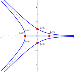
Figure 1: The saddle points (red dots) and steepest descent contours (blue thick lines) of $f_{\pm}\left(s\right)$ when $a=0$.

For $a=0$, we plot saddle points (red dots) of $f_{\pm}\left(s\right)$ and the steepest descent contours (blue thick lines) passing through them in FIG. 1. When $a>0$, more possible saddle points and poles could appear and these steepest descent contours could change dramatically around them, e.g. a contour that goes to infinity in the case $a=0$ could change to the one that ends at a new saddle point or a pole. However within $C_{R}$, there are no new saddle points or poles, and hence $C_{\lambda_{k}}$ would change continuously as $a$ is varied away from $0$. FIG. 1 shows that for $a=0$, $C_{\lambda_{2}}$ approaches $\theta=\frac{2\pi}{3}$ and $\frac{4\pi}{3}$ for a large value of $\left|s\right|$. So when $a>0$, $C_{\lambda_{2}}$ will intersect $C_{R}$ twice, and the intersections $Re^{i\theta_{\ast}}$ are within $\left|\theta^{\ast}-\frac{2\pi}{3}\right|\leq\frac{\pi}{18}+\mathcal{O}\left(a\right)$ and $\left|\theta^{\ast}-\frac{4\pi}{3}\right|\leq\frac{\pi}{18}+\mathcal{O}\left(a\right)$, respectively. Similarly, $C_{\lambda_{1}}$ intersects $C_{R}$ within $\left|\theta^{\ast}\right|\leq\frac{\pi}{18}+\mathcal{O}\left(a\right)$ and $\left|\theta^{\ast}-\frac{2\pi}{3}\right|\leq\frac{\pi}{18}+\mathcal{O}\left(a\right)$, $C_{\lambda_{3}}$ intersects $C_{R}$ within $\left|\theta^{\ast}\right|\leq\frac{\pi}{18}+\mathcal{O}\left(a\right)$ and $\left|\theta^{\ast}-\frac{4\pi}{3}\right|\leq\frac{\pi}{18}+\mathcal{O}\left(a\right)$, and $C_{\lambda_{0}}$ ends at $\lambda_{2}\left(a\right)$ and intersects $C_{R}$ within $\left|\theta^{\ast}\right|\leq\frac{\pi}{18}+\mathcal{O}\left(a\right)$.

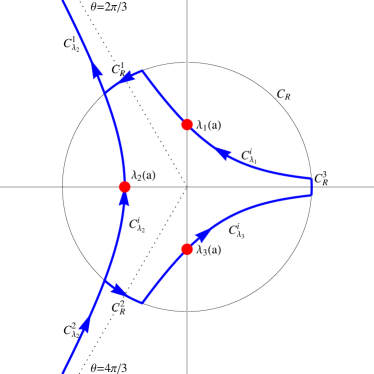
(a)  Contours of $\psi_{1}\left(\rho\right)$. The contour used in the $\rho>0$ $\left(\rho<0\right)$ case is the one passing through the saddle point(s) $\lambda_{2}\left(a\right)$ $\left(\lambda_{1}\left(a\right)\text{ and }\lambda_{3}\left(a\right)\right)$.

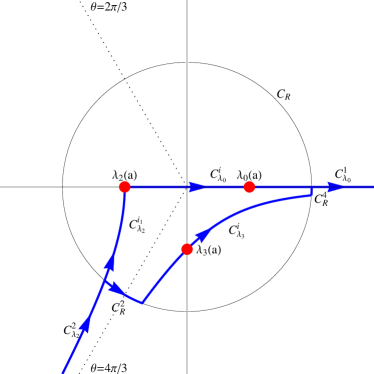
(b)  Contours of $\psi_{2}\left(\rho\right)$. The contour used in the $\rho>0$ $\left(\rho<0\right)$ case is the one passing through the saddle point(s) $\lambda_{0}\left(a\right)$ and $\lambda_{2}\left(a\right)$ $\left(\lambda_{3}\left(a\right)\right)$.

Figure 2: Contours (blue thick lines) and saddle points (red dots) of $\psi_{1}\left(\rho\right)$ and $\psi_{2}\left(\rho\right)$ in the $\rho>0$ and $\rho<0$ cases.

Since the saddle points and hence the solutions in eqn. $\left(\ref{eq:interalsolution}\right)$ depend on the sign of $\rho$, it is convenient to choose different contours in the complex plane for $\rho>0$ and $\rho<0$, making sure that they are deformable to each other. In FIG. 2(a), the contour considered in the $\rho>0$ case is the steepest descent contour $C_{\lambda_{2}}$ through $\lambda_{2}\left(a\right)$. For simplicity, we assume $\arg\lambda_{k}\left(a\right)=k\pi/2$ to illustrate the contours in FIG. 2. In FIG. 2, $C_{\lambda_{k}}^{i}$ denotes the part of $C_{\lambda_{k}}$ inside the circle $C_{R}$ while $C_{\lambda_{k}}^{1,2}$ denotes the parts of $C_{\lambda_{k}}$ outside $C_{R}$. Note that $f_{+}\left(s\right)\rightarrow-\infty$ when one moves away from the saddle point, and hence the corresponding integrand in eqn. $\left(\ref{eq:interalsolution}\right)$ vanishes at endpoints of $C_{\lambda_{2}}$. Since $C_{\lambda_{2}}$ is a steepest descent contour, when $1\ll\rho\ll\alpha^{-2}$, the dominant contribution to the integral over $C_{\lambda_{2}}$ in eqn. $\left(\ref{eq:interalsolution}\right)$ comes from the neighborhood of the saddle point $\lambda_{2}\left(a\right)$. Thus by the method of steepest descent, one has for $1\ll\rho\ll\tilde{\alpha}^{-2}$ that

$$\psi_{1}\left(\rho\right)=\left|\rho\right|^{\frac{1}{2}}\int_{C_{>}}\exp\left[\left|\rho\right|^{\frac{3}{2}}f_{+}\left(s\right)\right]ds\sim I_{\lambda_{2}\left(a\right)}\text{,}$$ (40)

where $C_{>}=C_{\lambda_{2}}$, and $I_{\lambda_{k}\left(a\right)}$ is the contribution from the saddle point $\lambda_{k}\left(a\right)$. Using Watson’s lemma, we find

$$I_{\lambda_{k}\left(a\right)}\sim\frac{\sqrt{\pi}\exp\left[\left|\rho\right|^{\frac{3}{2}}f_{\pm}\left(\lambda_{k}\left(a\right)\right)\right]}{\left|\rho\right|^{\frac{1}{4}}}\sqrt{\frac{2}{\left[s^{2}g^{2}\left(-ias\right)\right]^{\prime}|_{s=\lambda_{k}\left(a\right)}}},$$ (41)

where $k=0$ and $2$ is for $+$, and $k=1$ and $3$ for $-$. To study the asymptotic behavior of $\psi_{1}\left(\rho\right)$ when $-1\gg\rho\gg-\tilde{\alpha}^{-2}$, we consider

$$\psi_{1}\left(\rho\right)=\left|\rho\right|^{\frac{1}{2}}\int_{C_{<}}\exp\left[\left|\rho\right|^{\frac{3}{2}}f_{-}\left(s\right)\right]ds\text{,}$$ (42)

where the contour $C_{<}$ consists of $C_{\lambda_{2}}^{1}$, $C_{\lambda_{2}}^{2}$, $C_{\lambda_{1}}^{i}$, $C_{\lambda_{3}}^{i}$, $C_{R}^{1}$, $C_{R}^{2}$, and $C_{R}^{3}$, as shown in FIG. 2(a). Since the contributions from $C_{\lambda_{2}}^{1}$ and $C_{\lambda_{2}}^{2}$ are neglected in eqn. $\left(\ref{eq:phi1plus}\right)$, they can also be neglected in eqn. $\left(\ref{eq:phi1minus}\right)$. The contours $C_{R}^{i}$ connect two adjacent steepest descent contour along the circle $C_{R}$. Thus, propositions 27 and 2 implies that the contributions from $C_{R}^{i}$ is

$$\left|\left|\rho\right|^{\frac{1}{2}}\int_{C_{R}^{i}}\exp\left[\left|\rho\right|^{\frac{3}{2}}f_{-}\left(s\right)\right]ds\right|\sim\frac{\pi c\left|\rho\right|^{\frac{1}{2}}}{9a}\exp\left[-\frac{c^{3}\left|\rho\right|^{\frac{3}{2}}}{12a^{3}}\right],$$ (43)

where $i=1,2,3$. Since $\left|f_{-}\left(s\right)\right|\sim\mathcal{O}\left(1\right)$ at $s=\lambda_{1}\left(a\right)$ and $\lambda_{3}\left(a\right)$, the contributions from $C_{R}^{i}$ can also be neglected. Thus considering the contributions from $C_{\lambda_{1}}^{i}$ and $C_{\lambda_{3}}^{i}$ around the saddle points $\lambda_{1}\left(a\right)$ and $\lambda_{3}\left(a\right)$, we find that when $-1\gg\rho\gg-\tilde{\alpha}^{-2}$,

$$\psi_{1}\left(\rho\right)\sim I_{\lambda_{1}\left(a\right)}+I_{\lambda_{3}\left(a\right)}.$$ (44)

Since there is no singularity inside $C_{R}$, the contour $C_{<}$ used in the $\rho<0$ case can be deformed to $C_{>}$ in the $\rho>0$ case.

Similarly in FIG 2(b) , we consider the contour $C_{>}=C_{\lambda_{2}}^{2}+C_{\lambda_{2}}^{i_{1}}+C_{\lambda_{0}}^{i}+C_{\lambda_{0}}^{1}$ in the $\rho>0$ case and $C_{<}=C_{\lambda_{2}}^{2}+C_{R}^{2}+C_{\lambda_{3}}^{i}+C_{R}^{4}+C_{\lambda_{0}}^{1}$ in the $\rho<0$ case. It is noteworthy that the contours $C_{>}$ and $C_{<}$ are deformable to each other. As argued before, the contributions from $C_{R}^{2}$ and $C_{R}^{4}$ can be neglected. Since the leading contribution to the integral over a steepest descent contour comes from a small vicinity of the saddle point, the contributions from $C_{\lambda_{0}}^{1}$ and $C_{\lambda_{2}}^{2}$ can also be neglected. Moreover, $\lambda_{2}\left(a\right)$ is on the steepest descent contour $C_{\lambda_{0}}$ passing through $\lambda_{0}\left(a\right)$, and hence $\left|I_{\lambda_{2}\left(a\right)}\right|\ll$ $\left|I_{\lambda_{0}\left(a\right)}\right|$. So $I_{\lambda_{2}\left(a\right)}$ can be neglected for the integral over $C_{>}$. Therefore when $1\ll\rho\ll\tilde{\alpha}^{-2}$, the asymptotic behavior of the solution

$$\psi_{2}\left(\rho\right)=\left|\rho\right|^{\frac{1}{2}}\int_{C_{>}}\exp\left[\left|\rho\right|^{\frac{3}{2}}f_{-}\left(s\right)\right]ds,$$ (45)

is

$$\psi_{2}\left(\rho\right)\sim I_{\lambda_{0}\left(a\right)}\text{.}$$ (46)

When $-1\gg\rho\gg-\tilde{\alpha}^{-2}$, the asymptotic behavior of $\psi_{2}\left(\rho\right)$ is

$$\psi_{2}\left(\rho\right)\sim I_{\lambda_{3}\left(a\right)}\text{.}$$ (47)

To better illustrate the contours, we plot these contours for $g\left(x\right)=\frac{\tan\left(x\right)}{x}$ in the appendix.

Now suppose that $p^{2}\left(\xi\right)$ has a simple (first order) at $\xi=0$ and $F\equiv-\frac{dp^{2}\left(\xi\right)}{d\xi}|_{\xi=0}>0$. A linear approximation to the potential $p^{2}\left(\xi\right)$ near the turning point $\xi=0$ is

$$p^{2}\left(\xi\right)\approx-F\xi.$$ (48)

In the vicinity of $\xi=0$, if we make change of variables $\xi=\ell_{F}\rho$ and $\alpha=\ell_{F}\tilde{\alpha}\hbar^{-1}$, where $\ell_{F}=\hbar^{2/3}F^{-1/3}$, eqn. $\left(\ref{eq:DeformedEq}\right)$ becomes eqn. $\left(\ref{eq:linearDE}\right)$. Thus in the region where eqn. $\left(\ref{eq:linearp}\right)$ holds, we conclude that $\psi_{1}\left(\rho\right)$ and $\psi_{2}\left(\rho\right)$ are solutions of eqn. $\left(\ref{eq:DeformedEq}\right)$. On the other hand, we find for the linear approximation of $p^{2}\left(\xi\right)$ that

$$\frac{1}{\hbar}\int_{0}^{\xi}\left|p\left(\xi\right)\right|\lambda_{k}\left(\alpha\left|p\left(\xi\right)\right|\right)d\xi$$

$$=-\frac{\ell_{F}^{3}}{\hbar^{3}}\int_{0}^{\frac{\hbar}{\ell_{F}}\sqrt{-\rho}}\left|p\right|\lambda_{k}\left(\alpha\left|p\right|\right)d\left(p^{2}\right)$$

$$=-\frac{\ell_{F}^{3}}{\hbar^{3}}\left[-\frac{\hbar^{3}\rho\sqrt{\left|\rho\right|}}{\ell_{F}^{3}}\lambda_{k}\left(a\right)+\int_{0}^{\frac{\hbar}{\ell_{F}}\sqrt{\left|\rho\right|}\lambda_{k}\left(a\right)}u^{2}g^{2}\left(-i\alpha u\right)du\right]$$ (49)

$$=\left|\rho\right|^{\frac{3}{2}}\left[\text{sgn}\left(\rho\right)\lambda_{k}\left(a\right)-\int_{0}^{\lambda_{k}\left(a\right)}s^{2}g^{2}\left(-ias\right)ds\right]$$

$$=\left|\rho\right|^{\frac{3}{2}}f_{\pm}\left(\lambda_{k}\left(a\right)\right),$$

where we use eqn. $\left(\ref{eq:linearp}\right)$ for $p^{2}$ in the second line, $u=\left|p\right|\lambda_{k}\left(\alpha\left|p\right|\right)$ in the third line, and $s=u/\frac{\hbar}{\ell_{F}}\sqrt{\left|\rho\right|}$ in the fourth line. Defining $\alpha_{k}\left(a\right)$ and $\theta_{k}\left(a\right)$ as in

$$\lambda_{k}\left(a\right)=\left|\lambda_{k}\left(a\right)\right|e^{i\left(\pi k/2+\alpha_{k}\left(a\right)\right)}\text{ and }\theta_{k}\left(a\right)=\arg\left[1-ia\lambda_{k}^{2}\left(a\right)e^{-i\pi k/2}g^{\prime}\left(-ia\lambda_{k}\left(a\right)\right)\right],$$ (50)

one obtains for the linear approximation of $p^{2}\left(\xi\right)$ that

$$\left|\left[x^{2}g^{2}\left(\alpha x\right)\right]^{\prime}|_{x=-i\left|p\left(\xi\right)\right|\lambda_{k}\left(\alpha\left|p\left(\xi\right)\right|\right)}\right|=\frac{\hbar}{\ell_{F}}\sqrt{\left|\rho\right|}\left[s^{2}g^{2}\left(-ias\right)\right]^{\prime}|_{s=\lambda_{k}\left(a\right)}e^{-i\left(\pi k/2+\theta_{k}\left(a\right)-\alpha_{k}\left(a\right)\right)},$$ (51)

where $s=i\frac{\ell_{F}}{\hbar\sqrt{\left|\rho\right|}}x$. From eqns. $\left(\ref{eq:wkbI}\right)$ and $\left(\ref{eq:wkbF}\right)$, we have

$$\frac{\exp\left(\frac{1}{\hbar}\int\left|p\left(\xi\right)\right|\lambda_{k}\left(\alpha\left|p\left(\xi\right)\right|\right)d\xi\right)}{\sqrt{\left|\left[x^{2}g^{2}\left(\alpha x\right)\right]^{\prime}|_{x=-i\left|p\left(\xi\right)\right|\lambda_{k}\left(\alpha\left|p\left(\xi\right)\right|\right)}\right|}}\sim\sqrt{\frac{\ell_{F}}{2\pi\hbar}}C_{k}e^{i\left(\pi k/4+\theta_{k}\left(a\right)/2-\alpha_{k}\left(a\right)/2\right)}I_{\lambda_{k}\left(a\right)}.$$ (52)

When $\left|\xi\right|\ll F^{-1}\alpha^{-2}$ $\left(\alpha\left|p\left(\xi\right)\right|\ll 1\right)$, the condition $\left(\ref{eq:Condition}\right)$ for validity of the WKB approximation becomes

$$\left|\xi\right|\gg\ell_{F}\text{.}$$ (53)

In terms of $\rho$, the WKB solutions $\left(\ref{eq:wkbp>0}\right)$ and $\left(\ref{eq:wkbp<0}\right)$ for the linear approximation of $p^{2}\left(\xi\right)$ are valid when $\tilde{\alpha}^{-2}\gg\left|\rho\right|\gg$ $1$. However, we can approximate $\psi_{1}\left(\rho\right)$ and $\psi_{2}\left(\rho\right)$ by their leading asymptotic behaviors for $\tilde{\alpha}^{-2}\gg\left|\rho\right|\gg$ $1$. Since

$$I_{\lambda_{1}\left(a\right)}+I_{\lambda_{3}\left(a\right)}\overset{-1\gg\rho\gg-\tilde{\alpha}^{-2}}{\sim}\psi_{1}\left(\rho\right)\overset{1\ll\rho\ll\alpha^{-2}}{\sim}I_{\lambda_{2}\left(a\right)},$$ (54)

we use eqn. $\left(\ref{eq:matching}\right)$ to match WKB solutions $\left(\ref{eq:wkbp>0}\right)$ and $\left(\ref{eq:wkbp<0}\right)$ with $\psi_{1}\left(\rho\right)$ over the overlap region $\tilde{\alpha}^{-2}\gg\left|\rho\right|\gg$ $1$ and find that one connection formula around the turning point is

$$\psi_{WKB}\left(\xi\right)=\left\{\begin{array}[c]{c}Ce^{i\left[\alpha_{2}\left(a\right)/2-\theta_{2}\left(a\right)/2\right]}\psi_{WKB}^{2}\left(\xi\right)\text{ for }\xi>0\\ Ce^{i\left[\pi/4+\alpha_{1}\left(a\right)/2-\theta_{1}\left(a\right)/2\right]}\psi_{WKB}^{1}\left(\xi\right)+Ce^{i\left[-\pi/4+\alpha_{3}\left(a\right)/2-\theta_{3}\left(a\right)/2\right]}\psi_{WKB}^{3}\left(\xi\right)\text{ for }\xi<0\end{array}.\right.$$ (55)

Similarly for $\psi_{2}\left(\rho\right)$, we find that another connection formula is

$$\psi_{WKB}\left(\xi\right)=\left\{\begin{array}[c]{c}Ce^{i\left[\alpha_{0}\left(a\right)/2-\theta_{0}\left(a\right)/2\right]}\psi_{WKB}^{0}\left(\xi\right)\text{ for }\xi>0\\ Ce^{i\left[-3\pi/4+\alpha_{3}\left(a\right)/2-\theta_{3}\left(a\right)/2\right]}\psi_{WKB}^{3}\left(\xi\right)\text{ for }\xi<0\end{array}.\right.$$ (56)

II.3 Bohr-Sommerfeld Quantization and Tunneling Rates

In the usual quantum mechanics, the Bohr-Sommerfeld quantization condition and tunneling rates through potential barriers can be derived from the WKB connection formulas. However, more conditions are needed to be imposed on the function $g\left(x\right)$ to obtain the he Bohr-Sommerfeld quantization condition and tunneling rates in our case. In fact, we further require that $g\left(z\right)=g\left(-z\right)$ for $z\in C$, and both $g\left(x\right)$ and $\tilde{g}\left(x\right)\equiv g\left(ix\right)$ are real functions when $x\in R$. Note that $g\left(x\right)=1\pm x^{2}$ and $\tan x/x$ satisfy the above requirements. Under these requirements, the solutions $\lambda_{k}\left(a\right)$ of eqn. $\left(\ref{eq:lamda}\right)$ satisfies the properties:

1. $\lambda_{0}\left(a\right)=-\lambda_{2}\left(a\right)$ and $\lambda_{1}\left(a\right)=-\lambda_{3}\left(a\right)$,

2. For small enough value of $a$, one has that $\lambda_{k}\left(a\right)=\left|\lambda_{k}\left(a\right)\right|e^{ik\pi/2},$

where the second property comes from the fact that for any real function $f\left(x\right)$, the equation $xf\left(ax\right)=1$ always has a real solution around $x=1$ if $a$ is small enough. Furthermore, these properties imply that $\theta_{k}\left(a\right)=\alpha_{k}\left(a\right)=0$. In the region $\xi>0\,\$where $p^{2}\left(\xi\right)<0$, $\psi_{WKB}^{0}\left(\xi\right)$ is exponentially increasing away from the turning point $\xi=0$ while $\psi_{WKB}^{2}\left(\xi\right)$ is exponentially decreasing. In the region $\xi<0\,\$where $p^{2}\left(\xi\right)>0$, $\psi_{WKB}^{1}\left(\xi\right)$ and $\psi_{WKB}^{3}\left(\xi\right)$ are oscillatory solutions and propagate toward and away from the turning point, respectively.

Now suppose that $p^{2}\left(\xi\right)$ has two simple points at $\xi=A$ and $\xi=B$ with $A<B$. We also assume that $p^{2}\left(\xi\right)<0$ if $\xi>B$ or $\xi<A$, and that $p^{2}\left(\xi\right)>0$ if $A<\xi<B$. To study the boundary-value problem with $\psi\left(\pm\infty\right)=0$, we consider the two-turning-point solutions by matching two one-turning-point solutions: the first one is from $+\infty$ through $B$ and down to near $A$; the second is $-\infty$ through $A$ and down to near $B$. We can use the WKB connection formula $\left(\ref{eq:wkbC1}\right)$ to show that the first one-turning-point solution that decays like

$$C\psi_{WKB}^{2}\left(\xi\right)=\frac{C\exp\left(\frac{1}{\hbar}\int_{B}^{\xi}\left|p\left(\xi^{\prime}\right)\right|\lambda_{2}\left(\alpha\left|p\left(\xi^{\prime}\right)\right|\right)d\xi^{\prime}\right)}{\sqrt{\left|\left[x^{2}g^{2}\left(\alpha x\right)\right]^{\prime}|_{x=i\left|p\left(\xi\right)\right|\lambda_{2}\left(\alpha\left|p\left(\xi\right)\right|\right)}\right|}},$$ (57)

as $\xi\rightarrow+\infty$ behaves like

$$\frac{2C}{\sqrt{\left|\left[x^{2}g^{2}\left(\alpha x\right)\right]^{\prime}|_{x=\left|p\left(\xi\right)\lambda_{1}\left(\alpha\left|p\left(\xi\right)\right|\right)\right|}\right|}}\sin\left(\frac{1}{\hbar}\int_{\xi}^{B}\left|p\left(\xi^{\prime}\right)\lambda_{1}\left(\alpha\left|p\left(\xi^{\prime}\right)\right|\right)\right|d\xi^{\prime}+\frac{\pi}{4}\right)$$

$$=-\frac{2C\sin\left[\frac{1}{\hbar}\int_{A}^{\xi}\left|p\left(\xi^{\prime}\right)\lambda_{1}\left(\alpha\left|p\left(\xi^{\prime}\right)\right|\right)\right|d\xi^{\prime}+\frac{\pi}{4}-\left\{\frac{1}{\hbar}\int_{A}^{B}\left|p\left(\xi^{\prime}\right)\lambda_{1}\left(\alpha\left|p\left(\xi^{\prime}\right)\right|\right)\right|d\xi^{\prime}+\frac{\pi}{2}\right\}\right]}{\sqrt{\left|\left[x^{2}g^{2}\left(\alpha x\right)\right]^{\prime}|_{x=\left|p\left(\xi\right)\lambda_{1}\left(\alpha\left|p\left(\xi\right)\right|\right)\right|}\right|}},$$ (58)

in the region between $A$ and $B$. Similarly, the second one-turning-point solution that decays like

$$\frac{C^{\prime}\exp\left(\frac{1}{\hbar}\int_{\xi}^{A}\left|p\left(\xi^{\prime}\right)\right|\lambda_{2}\left(\alpha\left|p\left(\xi^{\prime}\right)\right|\right)d\xi^{\prime}\right)}{\sqrt{\left|\left[x^{2}g^{2}\left(\alpha x\right)\right]^{\prime}|_{x=i\left|p\left(\xi\right)\right|\lambda_{2}\left(\alpha\left|p\left(\xi\right)\right|\right)}\right|}},$$ (59)

as $\xi\rightarrow-\infty$ behaves like

$$\frac{2C^{\prime}}{\sqrt{\left|\left[x^{2}g^{2}\left(\alpha x\right)\right]^{\prime}|_{x=\left|p\left(\xi\right)\lambda_{1}\left(\alpha\left|p\left(\xi\right)\right|\right)\right|}\right|}}\sin\left(\frac{1}{\hbar}\int_{A}^{\xi}\left|p\left(\xi^{\prime}\right)\lambda_{1}\left(\alpha\left|p\left(\xi^{\prime}\right)\right|\right)\right|d\xi^{\prime}+\frac{\pi}{4}\right),$$ (60)

in the region between $A$ and $B$. In order that the two solutions in eqns. $\left(\ref{eq:wkbAB}\right)$ and $\left(\ref{eq:wkbBA}\right)$ match over the region between $A$ and $B$, we require that the expression in the curly bracket of eqn. $\left(\ref{eq:wkbAB}\right)$ is an integral multiple of $\pi$. Therefore, we derive the Bohr-Sommerfeld quantization condition:

$$\frac{1}{\hbar}\int_{A}^{B}\left|p\left(\xi\right)\lambda_{1}\left(\alpha\left|p\left(\xi\right)\right|\right)\right|d\xi=\left(n+\frac{1}{2}\right)\pi+\mathcal{O}\left(\hbar\right),$$ (61)

where $n$ is a nonnegative integer.

We now consider WKB description of tunneling, in which $p\left(-\infty\right)=$ $p\left(+\infty\right)>0$ and $p^{2}\left(\xi\right)$ vanishes at two turning points $x=A\$and $x=B$. Moreover, there are two classical allowed regions $p^{2}\left(\xi\right)>0$, Region I with $\xi<A$ and Region III with $\xi>B$, and one forbidden region $p^{2}\left(\xi\right)<0$, Region II with $A<\xi<B$. To describe tunneling, we need to choose appropriate boundary conditions in the classical allowed regions. We postulate that there is only a transmitted wave in Region III:

$$F\psi_{WKB}^{3}\left(\xi\right) =\frac{F\exp\left(\frac{1}{\hbar}\int_{0}^{B-\xi}\left|p\left(B-\xi^{\prime}\right)\right|\lambda_{3}\left(\alpha\left|p\left(B-\xi^{\prime}\right)\right|\right)d\xi^{\prime}\right)}{\sqrt{\left|\left[x^{2}g^{2}\left(\alpha x\right)\right]^{\prime}|_{x=\left|p\left(\xi\right)\lambda_{3}\left(\alpha\left|p\left(\xi\right)\right|\right)\right|}\right|}}$$

$$=\frac{F\exp\left(\frac{i}{\hbar}\int_{B}^{\xi}\left|p\left(\xi^{\prime}\right)\lambda_{1}\left(\alpha\left|p\left(\xi^{\prime}\right)\right|\right)\right|d\xi^{\prime}\right)}{\sqrt{\left|\left[x^{2}g^{2}\left(\alpha x\right)\right]^{\prime}|_{x=\left|p\left(\xi\right)\lambda_{1}\left(\alpha\left|p\left(\xi\right)\right|\right)\right|}\right|}}.$$ (62)

Using the WKB connection formula $\left(\ref{eq:wkbC2}\right)$, we find that the WKB solution in Region II is

$$\frac{Fe^{3i\pi/4}\exp\left(\frac{1}{\hbar}\int_{\xi}^{B}\left|p\left(\xi^{\prime}\right)\right|\lambda_{0}\left(\alpha\left|p\left(\xi^{\prime}\right)\right|\right)d\xi^{\prime}\right)}{\sqrt{\left|\left[x^{2}g^{2}\left(\alpha x\right)\right]^{\prime}|_{x=i\left|p\left(\xi\right)\right|\lambda_{0}\left(\alpha\left|p\left(\xi\right)\right|\right)}\right|}}=\frac{Fe^{3i\pi/4}e^{\eta}\exp\left(\frac{1}{\hbar}\int_{A}^{\xi}\left|p\left(\xi^{\prime}\right)\right|\lambda_{2}\left(\alpha\left|p\left(\xi^{\prime}\right)\right|\right)d\xi^{\prime}\right)}{\sqrt{\left|\left[x^{2}g^{2}\left(\alpha x\right)\right]^{\prime}|_{x=i\left|p\left(\xi\right)\right|\lambda_{0}\left(\alpha\left|p\left(\xi\right)\right|\right)}\right|}},$$ (63)

where

$$\eta=\frac{1}{\hbar}\int_{A}^{B}\left|p\left(\xi\right)\right|\lambda_{0}\left(\alpha\left|p\left(\xi\right)\right|\right)d\xi.$$ (64)

In Region I, the WKB approximation solution includes a wave incident the barrier and a reflected wave:

$$\frac{Fe^{\eta}\left[e^{i\pi/2}\exp\left(\frac{i}{\hbar}\int_{A}^{\xi}\left|p\left(\xi^{\prime}\right)\lambda_{1}\left(\alpha\left|p\left(\xi^{\prime}\right)\right|\right)\right|d\xi^{\prime}\right)+e^{i\pi}\exp\left(-\frac{i}{\hbar}\int_{A}^{\xi}\left|p\left(\xi^{\prime}\right)\lambda_{1}\left(\alpha\left|p\left(\xi^{\prime}\right)\right|\right)\right|d\xi^{\prime}\right)\right]}{\sqrt{\left|\left[x^{2}g^{2}\left(\alpha x\right)\right]^{\prime}|_{x=\left|p\left(\xi\right)\lambda_{1}\left(\alpha\left|p\left(\xi\right)\right|\right)\right|}\right|}},$$ (65)

where the first term in the square bracket is the incident wave with the amplitude $A=Fe^{\eta}e^{i\pi/2}$. Therefore, the transmission probability is

$$T=\frac{\left|F\right|^{2}}{\left|A\right|^{2}}\sim e^{-2\eta}.$$ (66)

III Examples

In this section, we use the results obtained in the previous section to discuss some interesting examples in the deformed quantum mechanics. To compare results in the literature, we first show that how a deformed Schrodinger-like equation appears in the two effective models of quantum gravity mentioned in Introduction. The first one is the GUP IN-Maggiore:1993kv ; IN-Kempf:1994su , derived from the modified fundamental commutation relation:

$$[X,P]=i\hbar f\left(P\right),$$ (67)

where $f\left(P\right)$ is some function. This model is inspired by the prediction of the existence of a minimal length in various theories of quantum gravity, such as string theory, loop quantum gravity and quantum geometry IN-Townsend:1977xw ; IN-Amati:1988tn ; IN-Konishi:1989wk . For example, if $f\left(P\right)=1+\beta P^{2}$, the minimal measurable length is

$$l_{\min}=\hbar\sqrt{\beta}.$$ (68)

The GUP has been extensively studied recently, see for example IN-Chang:2001bm ; IN-Brau:1999uv ; IN-Das:2008kaa ; IN-Hossenfelder:2003jz ; IN-Ali:2009zq ; IN-Li:2002xb ; IN-Brau:2006ca ; IN-Scardigli:1999jh ; IN-Scardigli:2014qka . For a review of the GUP, see IN-Chen:2014xgj ; IN-Hossenfelder:2012jw . To study 1D quantum mechanics with the deformed commutators $(\ref{eq:1dGUP})$, one can exploit the following representation for $X$ and $P$ in the the position representation:

$$X=X_{0}\text{ and }P=P\left(\frac{\hbar}{i}\frac{\partial}{\partial x}\right),$$ (69)

where the function $P\left(x\right)$ is the solution of the differential equation $\frac{dP\left(x\right)}{dx}=f\left(P\right)$. Usually, we could write $P\left(x\right)$ in terms of the function $g\left(x\right)$ as

$$P\left(x\right)=xg\left(\alpha x\right),$$ (70)

where $\alpha$ is a parameter and can be related to the minimal length: $l_{\min}=\hbar\alpha$. In the $f\left(P\right)=1+\beta P^{2}$ case, one finds that

$$g\left(x\right)=\frac{\tan\left(x\right)}{x},$$ (71)

with $\alpha=\sqrt{\beta}$.

The second is the MDR. It is believed that the trans-Planckian physics manifests itself in certain modifications of the existing models. Thus, even though a complete theory of quantum gravity is not yet available, we can use a “bottom-to-top approach” to probe the possible effects of quantum gravity on our current theories and experiments IN-AmelinoCamelia:2004hm . One possible way of how such an approach works is via Planck-scale modifications of the usual energy-momentum dispersion relation

$$p^{2}=E^{2}-m^{2},$$ (72)

whose possibility has been considered in the quantum-gravity literature IN-AmelinoCamelia:1997gz ; IN-Garay:1998wk ; IN-AmelinoCamelia:2002wr ; IN-Magueijo:2002am . The modified dispersion relation (MDR) has been reviewed in the framework of Lorentz violating theories in IN-Mattingly:2005re ; IN-Liberati:2013xla . It has also been shown that the MDR might play a role in astronomical and cosmological observations, such as the threshold anomalies of ultra high energy cosmic rays and TeV photons IN-AmelinoCamelia:1997gz ; IN-Colladay:1998fq ; IN-Coleman:1998ti ; IN-AmelinoCamelia:2000zs ; IN-Jacobson:2001tu ; IN-Jacobson:2003bn . In most cases, the MDR could take the form

$$E^{2}=p^{2}g^{2}\left(\alpha p\right)+m^{2},$$ (73)

where $\alpha=\Lambda^{-1}$, and $\Lambda$ is the cut off scale which characterizes the new physics in Planck scale. To obtain the deformed wave equations, we can define the modified differential operator by

$$P=P_{0}g\left(\alpha P_{0}\right),$$ (74)

where $P_{0}=\frac{\hbar}{i}\frac{\partial}{\partial x}$, and replace $P_{0}$ with $P$ IN-Corley:1996ar ; IN-Pavlopoulos:1967dm . Another way to obtain eqn. $\left(\ref{eq:pp0}\right)$ is using effective field theories (EFT). In fact, one has to break or modify the global Lorentz symmetry in the classical limit of the quantum gravity to have a MDR. There are several possibilities for breaking or modifying the Lorentz symmetry, one of which is that Lorentz invariance is spontaneously broken by extra tensor fields taking on vacuum expectation values IN-Colladay:1998fq . The most conservative approach for a framework in which to describe MDR is considering an EFT, in which modifications to the dispersion relation can be described by the higher dimensional operators. In In-Wang:2015lqa , we constructed a such EFT for a scalar field, which only contained the kinetic terms and the usual minimal gravitational couplings. It showed for the MDR $\left(\ref{eq:MDR}\right)$ that the deformed Klein-Gordon equation could be obtained via making the replacement $\left(\ref{eq:pp0}\right)$. In this section, we take Planck units $c=G=\hbar=k=1$.

III.1 Harmonic Oscillator

We first study a simple example, bound states of an harmonic oscillator in the potential $V\left(x\right)=\frac{m\omega^{2}x^{2}}{2}$. For the harmonic oscillator, the deformed Schrodinger equation is

$$\left[-\partial_{x}^{2}g^{2}\left(-i\alpha\partial_{x}\right)-p^{2}\left(x\right)\right]\psi\left(x\right)=0,$$ (75)

where $p^{2}\left(x\right)=m^{2}\omega^{2}\left(x_{0}^{2}-x^{2}\right)$ and $x_{0}=\sqrt{\frac{2E}{m\omega^{2}}}$. Considering $g\left(x\right)=\frac{\tan\left(x\right)}{x}$, one then has

$$\lambda_{1}\left(a\right)=\frac{i}{a}\arctan a.$$ (76)

In this case, the Bohr-Sommerfeld quantization condition becomes

$$2\int_{0}^{x_{0}}\left|p\left(x\right)\frac{i}{\alpha\left|p\left(x\right)\right|}\arctan\left(\alpha\left|p\left(x\right)\right|\right)\right|dx=\left(n+\frac{1}{2}\right)\pi,$$ (77)

which gives the energy levels of bound states

$$E_{n}=E_{0,n}\left(1+\frac{\alpha^{2}mE_{0,n}}{2}\right),$$ (78)

for $n=0,1,2\cdots$, where $E_{0,n}=\left(n+\frac{1}{2}\right)\omega$.

In EX-Chang:2001kn , the differential equation $\left(\ref{eq:HOeqn}\right)$ with $g\left(x\right)=\frac{\tan\left(x\right)}{x}$ was solved exactly in the momentum space, and the exact energy levels were given by

$$E_{n} =\omega\left[\left(n+\frac{1}{2}\right)\sqrt{1+\frac{\beta^{2}m^{2}\omega^{2}}{4}}+\left(n^{2}+n+\frac{1}{2}\right)\frac{\beta m\omega}{2}\right]$$

$$=E_{0,n}\left[\sqrt{1+\alpha^{4}m^{2}E_{0,n}^{2}\left(\frac{\omega}{2E_{0,n}}\right)^{2}}+\frac{\alpha^{2}mE_{0,n}}{2}+\frac{\alpha^{2}mE_{0,n}}{2}\left(\frac{\omega}{2E_{0,n}}\right)^{2}\right],$$ (79)

where $\beta$ in EX-Chang:2001kn is our $\alpha^{2}$. The WKB approximation is a good approximation when the de Broglie wavelength $\lambda$ of a particle is smaller than the characteristic length $L$ of the potential. Thus, the higher order WKB corrections are suppressed by powers of $\frac{\lambda}{L}$ relative to the leading term. For the harmonic oscillator in the $n$th energy level, we find that

$$\frac{\lambda}{L}\sim\frac{\frac{1}{\sqrt{2mE_{0,n}}}}{x_{0}}=\frac{\omega}{2E_{0,n}}\text{.}$$ (80)

Therefore, the terms proportional to $\left(\frac{\omega}{2E_{0,n}}\right)^{2}$ in eqn. $\left(\ref{eq:HOexact}\right)$ are the higher order corrections, and hence the WKB result $\left(\ref{eq:HOWKB}\right)$ agrees with the leading term of the WKB expansion of the exact result $\left(\ref{eq:HOexact}\right)$. It is noteworthy that the momentum representation of the position operator is quadratic in the $g\left(x\right)=\frac{\tan\left(x\right)}{x}$ case, and hence eqn. $\left(\ref{eq:HOeqn}\right)$ can be solved exactly. However for a generic case, the WKB approximation could provide a simple way to estimate the quantum gravity’s corrections.

III.2 Schwinger Effect

The Schwinger effect EX-Schwinger:1951nm is an example of creation of particles by external fields, which consists in the creation of electron–positron pairs by a strong electric field. The WKB approximation and the Dirac sea picture can be used to illustrate its main physical features in a heuristic way. Suppose the electrostatic potential is

$$V\left(x\right)=\left\{\begin{array}[c]{l}0\text{ \ \ \ \ \ \ \ \ }x<0\\ -\mathcal{E}x\text{ \ \ \ }0<x<L\\ -\mathcal{E}L\text{\ \ \ }L<x\end{array}\right..$$ (81)

If $e\mathcal{E}L>2m$, there exist states in the Dirac sea with $x>L$ having the same energy as some positive energy states in the region $x<0$. The electrons with energy $m\leq E\leq e\mathcal{E}L-m$ in the Dirac sea could tunnel through the classically forbidden region leaving a hole behind, which can be described as the production of an electron–positron pair out of the vacuum by the effect of the electric field.

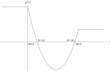
(a)  The plot of $p^{2}\left(x\right)$ for the Schwinger effect.

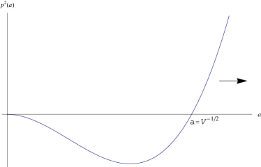
(b)  The plot of $p^{2}\left(a\right)$ for quantum cosmology.

Figure 3: The plot of $p^{2}\left(x\right)$ and $p^{2}\left(a\right)$.

For simplicity, we assume that electrons are described by a wave function $\Psi\left(t,x\right)$ satisfying the $1+1$ dimensional deformed Klein-Gordon equation

$$\left\{\left[i\partial_{t}+eV\left(x\right)\right]^{2}-\left(i\partial_{x}\right)^{2}g^{2}\left(-i\alpha\partial_{x}\right)-m^{2}\right\}\Psi\left(t,x\right)=0.$$ (82)

Since the potential only depends on $x$, we could the following ansatz for $\Psi\left(t,x\right)$

$$\Psi\left(t,x\right)=e^{-iEt}\psi\left(x\right).$$ (83)

Substituting this expression in eqn. $\left(\ref{eq:KG}\right)$ results in a deformed Schrodinger-like equation

$$-\partial_{x}^{2}g^{2}\left(-i\alpha\partial_{x}\right)\psi\left(x\right)-p^{2}\left(\xi\right)\psi\left(x\right)=0,$$ (84)

where $p^{2}\left(x\right)=\left[E+eV\left(x\right)\right]^{2}-m^{2}$. The function $p^{2}\left(x\right)$ has two turning points:

$$x_{\pm}=\frac{1}{e\mathcal{E}}\left(E\pm m\right),$$ (85)

where $0<x_{\_}<x_{+}<L$ since $m\leq E\leq e\mathcal{E}L-m$. We plot $p^{2}\left(x\right)$ in FIG. 3(a). Then, the WKB transmission coefficient is given by

$$T=\exp\left[-2\int_{x_{\_}}^{x_{+}}\left|p\left(x\right)\right|\lambda_{0}\left(\alpha\left|p\left(x\right)\right|\right)dx\right].$$ (86)

The number of pairs produced per unit time with energies between $E$ and $E+dE$ is

$$\frac{dN}{dt}=2T\frac{dE}{2\pi},$$ (87)

where the factor of $2$ takes into account the two polarizations of the electron. Note that the turning points $x_{\pm}$ are the positions at which the two particles of the pair are produced. Therefore, shifting the energy by $dE$ results in a change in the positions of the particles by $dx=\frac{dE}{e\mathcal{E}}$. It follows from eqn. $\left(\ref{eq:dn/dt}\right)$ that the pair production rate per unit length is

$$W=\frac{e\mathcal{E}}{\pi}T\text{.}$$ (88)

Considering the $g\left(x\right)=\tan\left(x\right)/x$ case in which $\lambda_{0}\left(a\right)=$arctanh$\left(a\right)/a$, we find

$$T=\exp\left[-\frac{2\pi}{e\mathcal{E}\alpha^{2}}\left(1-\sqrt{1-m^{2}\alpha^{2}}\right)\right].$$ (89)

Thus, the pair production rate per unit length is

$$W=\frac{e\mathcal{E}}{\pi}\exp\left[-\frac{2\pi}{e\mathcal{E}\alpha^{2}}\left(1-\sqrt{1-m^{2}\alpha^{2}}\right)\right].$$ (90)

The Schwinger mechanism can explain the Unruh effect which predicts that an accelerating observer will observe a thermal spectrum of photons and particle–antiparticle pairs at temperature $T=\frac{a}{2\pi},$ where $a$ is the acceleration EX-Unruh:1976db . In fact, considering a free particle of charge $e$ and mass $m$ moving in a static electric field $\mathcal{E}$, one finds that the acceleration of the particle is $a=\frac{em}{\mathcal{E}}$. It follows that the pair production rate per unit length is

$$W\sim\left[-\frac{K}{a/2\pi}\frac{1-\sqrt{1-4K^{2}\alpha^{2}}}{2K^{2}\alpha^{2}}\right],$$ (91)

where we identify the reduced mass $\frac{m}{2}=K$ as the energy associated with the pair production process. The Unruh temperature reads

$$T_{u}\sim\frac{a}{2\pi}\frac{2K^{2}\alpha^{2}}{1-\sqrt{1-4K^{2}\alpha^{2}}}.$$ (92)

For a Schwarzschild black hole of the mass $M$, the event horizon is at $r_{h}=2M$. Since the gravitational acceleration at the event horizon is given by

$$a=\frac{M}{r_{h}^{2}}=\frac{1}{4M},$$ (93)

it follows from eqn. $\left(\ref{eq:unruhT}\right)$ that the Hawking temperature is

$$T_{h}\sim T_{0}\frac{2T_{h}^{2}\alpha^{2}}{1-\sqrt{1-4T_{h}^{2}\alpha^{2}}},$$ (94)

where $T_{0}=\frac{1}{8\pi M}$, and we estimate that the energy of radiated particles $K\sim T_{h}$. Solving the above equation for $T_{h}$ gives

$$T_{h}=\frac{T_{0}}{1+\alpha^{2}T_{0}^{2}},$$ (95)

which shows that in the $g\left(x\right)=\tan\left(x\right)/x$ case, the quantum gravity effects always lower the Hawking temperature. Using the first law of the black hole thermodynamics, we find that the black hole’s entropy is

$$S=\int\frac{dM}{T_{h}}\sim\frac{A}{4}+\frac{\alpha^{2}}{8\pi}\ln\left(\frac{A}{16\pi}\right),$$ (96)

where $A=4\pi r_{h}^{2}=16\pi M^{2}$ is the area of the horizon.

III.3 Pöschl-Teller Potential and Quasinormal Modes of A Black Hole

It has been long known that the usual Schrodinger equation for the Pöschl–Teller potential of the form

$$V_{PT}\left(x,b\right)=-\frac{V_{0}}{\cosh^{2}bx},$$ (97)

is exactly solvable. For a particle of the mass $m=1/2$, the exact bound states are given by

$$E_{n}\left(b\right)=-b^{2}\left[-\left(n+\frac{1}{2}\right)+\left(\frac{1}{4}+\frac{V_{0}}{b^{2}}\right)^{\frac{1}{2}}\right]^{2},$$ (98)

for $n=0,1,2,\cdots,N-1$, where $N+\frac{1}{2}>\left(\frac{1}{4}+\frac{V_{0}}{b^{2}}\right)^{\frac{1}{2}}$. We now use the WKB method to solve the deformed Schrodinger equation for the bound states in the Pöschl–Teller potential. The deformed Schrodinger equation is given by

$$-\partial_{x}^{2}g^{2}\left(-i\alpha\partial_{x}\right)\Psi\left(x,b\right)+\left[V_{PT}\left(x,b\right)-E\left(b\right)\right]\Psi\left(x,b\right)=0.$$ (99)

The Bohr-Sommerfeld quantization condition $\left(\ref{eq:BS}\right)$ then leads to

$$\int_{-x_{0}}^{x_{0}}\left|p\left(x\right)\lambda_{1}\left(\alpha\left|p\left(x\right)\right|\right)\right|dx\approx\left(n+\frac{1}{2}\right)\pi,$$ (100)

where $x=\pm x_{0}\equiv\pm b^{-1}$arccosh$\left(\frac{V_{0}^{1/2}}{\sqrt{-E}}\right)$ are the turning points, and $p\left(x\right)=\sqrt{E-V_{PT}\left(x,b\right)}$.

Now consider the $g_{\pm}\left(x\right)=1\pm x^{2}$ case , in which we find that the solutions of $sg_{\pm}\left(-ias\right)=i$ are

$$\lambda_{1}^{\pm}\left(a\right)=i\left(1\pm a^{2}\right)+\mathcal{O}\left(a^{4}\right).$$ (101)

Solving eqn. $\left(\ref{eq:PTBS}\right)$ for $E$, we find that the bound states are

$$E_{n}^{\pm}\left(b\right)\approx-b^{2}\left[-\left(n+\frac{1}{2}\right)+\left(\frac{V_{0}}{b^{2}}\right)^{\frac{1}{2}}\mp\alpha^{2}b^{2}\left(n+\frac{1}{2}\right)^{2}\left(n+\frac{1}{2}-\frac{3}{2}\left(\frac{V_{0}}{b^{2}}\right)^{\frac{1}{2}}\right)\right]^{2},$$ (102)

where $n=0,1,2,\cdots$ such that the sum of terms in the square bracket is non-negative. If $\alpha=0$, from comparing the exact result $\left(\ref{eq:PTExact}\right)$ with the WKB one $\left(\ref{eq:PTWKB}\right)$, it follows that the higher WKB corrections are suppressed by powers of $b^{2}V_{0}^{-1}$. Therefore, combining results from eqns. $\left(\ref{eq:PTExact}\right)$ and $\left(\ref{eq:PTWKB}\right)$, one obtains the bound states:

$$E_{n}^{\pm}\left(b\right) =-b^{2}\left[-\left(n+\frac{1}{2}\right)+\left(\frac{1}{4}+\frac{V_{0}}{b^{2}}\right)^{\frac{1}{2}}\right.$$

$$\left.\mp\alpha^{2}b^{2}\left(n+\frac{1}{2}\right)^{2}\left(n+\frac{1}{2}-\frac{3}{2}\left(\frac{V_{0}}{b^{2}}\right)^{\frac{1}{2}}+\mathcal{O}\left(bV_{0}^{-1/2}\right)\right)+\mathcal{O}\left(\alpha^{4}b^{4}\right)\right]^{2}.$$ (103)

To study quasinormal modes of a static and spherically symmetric, we consider the propagation of the massless and minimally coupled scalar particles in a general Schwarzschild-like metric:

$$ds^{2}=h\left(r\right)dr^{2}-\frac{dr^{2}}{h\left(r\right)}-r^{2}d\Omega,$$ (104)

where $d\Omega$ is the solid angle. The wave equation for the scalar particles is the Klein-Gordon equation. After the wave function $\Psi\left(t,r,\Omega\right)$ is decomposed into eigenmodes of normal frequency $\omega$ and angular momentum $l$, $\Psi\left(t,r,\Omega\right)=e^{-i\omega t}Y_{l}^{m}\left(\Omega\right)R\left(r\right)/r$, the Klein-Gordon equation gives a Schrodinger-like equation for $R\left(r\right)$ in stationary backgrounds:

$$-\frac{d^{2}R\left(r_{\ast}\right)}{dr_{\ast}^{2}}+V\left(r_{\ast}\right)R=\omega^{2}R\left(r_{\ast}\right),$$ (105)

where $dr_{\ast}=dr/h\left(r\right)$ is the tortoise coordinate, and

$$V\left(r_{\ast}\right)=h\left(r\right)\left(\frac{l\left(l+1\right)}{r^{2}}+\frac{1}{r}\frac{dh}{dr}\right).$$ (106)

For asymptotically flat black holes, quasinormal modes are solutions of the wave equation $\left(\ref{eq:scheq}\right)$, satisfying specific boundary conditions EX-Konoplya:2011qq

$$R\sim e^{\pm i\omega r_{\ast}}\text{, }r_{\ast}\rightarrow\pm\infty.$$ (107)

In deformed quantum mechanics, the Schrodinger-like equation $\left(\ref{eq:scheq}\right)$ could be changed to

$$\left[-\frac{d^{2}}{dr_{\ast}^{2}}g^{2}\left(\alpha\frac{d}{idr_{\ast}}\right)+V\left(r_{\ast}\right)-\omega^{2}\right]R\left(r_{\ast}\right)=0.$$ (108)

The quasinormal modes can be estimated by using a simpler potential $-V_{PT}\left(x,b\right)$ that approximates $\left(\ref{eq:V}\right)$ closely, especially near its maximum EX-Ferrari:1984zz . The quantities $V_{0}$ and $b$ are given by the height and curvature of the potential $V\left(r\right)$ at its maximum $r_{\ast}=r_{\ast,0}$:

$$V_{0}=V\left(r_{\ast,0}\right)\text{ and }b^{2}=-\frac{1}{2V_{0}}\frac{d^{2}V\left(r_{\ast}\right)}{dr_{\ast}^{2}}|_{r_{\ast}=r_{\ast,0}}\text{.}$$ (109)

For a Schwarzschild black hole with $h\left(r\right)=1-\frac{2M}{r}$, we find

$$V_{0} =\frac{4l^{3}\left(l+1\right)^{3}\left(a_{l}-3-l-l^{2}\right)\left[1+3l\left(l+1\right)+a_{l}\right]}{\left[3l\left(l+1\right)-3+a_{l}\right]^{4}M^{2}},$$ (110)

$$b^{2} =\frac{16l^{2}\left(l+1\right)^{2}\left\{9\left(-3+a_{l}\right)+l\left(l+1\right)\left[-33+4a_{l}+l\left(l+1\right)\left(-13+9l\left(l+1\right)+3a_{l}\right)\right]\right\}}{\left[-3+3l\left(l+1\right)+{}a_{l}\right]^{4}\left[1+3l\left(l+1\right)+{}a_{l}\right]M^{2}},$$ (111)

where

$$a_{l}=\sqrt{9+l\left(l+1\right)\left(14+9l\left(l+1\right)\right)}\text{.}$$ (112)

Note that the ratio $bV_{0}^{-1/2}$ controlling the WKB expansion is given by

$$bV_{0}^{-1/2}\sim l^{-1}\text{.}$$ (113)

In this approximation, eqn. $\left(\ref{eq:deformedScheq}\right)$ becomes

$$\left[-\frac{d^{2}}{dr_{\ast}^{2}}g^{2}\left(\alpha\frac{d}{idr_{\ast}}\right)-V_{PT}\left(r_{\ast},b\right)-\omega^{2}\left(b\right)\right]R\left(r_{\ast},b\right)=0.$$ (114)

To relate the quasinormal modes of the above equation to the bound states of the Pöschl–Teller potential, we consider the formal transformations EX-Ferrari:1984zz

$$x\rightarrow-ir_{\ast}\text{ and }b\rightarrow ib$$ (115)

such that $V_{PT}\left(x,b\right)=V_{PT}\left(-ir_{\ast},ib\right)$. Let us define

$$\Psi\left(x,b\right) =R\left(-ix,ib\right),$$

$$E\left(b\right) =-\omega^{2}\left(ib\right).$$ (116)

Then $\Psi\left(x,b\right)$ satisfies

$$-\partial_{x}^{2}\tilde{g}^{2}\left(-i\alpha\partial_{x}\right)\Psi\left(x,b\right)+\left[V_{PT}\left(x,b\right)-E\left(b\right)\right]\Psi\left(x,b\right)=0,$$ (117)

where $\tilde{g}\left(x\right)=g\left(-ix\right)$, and the boundary conditions for the quasinormal modes are reduced to

$$\Psi\left(x,b\right)\sim\exp\left(\mp\sqrt{-E\left(b\right)}x\right)\text{, as }x\rightarrow\pm\infty.$$ (118)

The quasinormal modes in the $g\left(x\right)$ case can be found by the bound states of the Pöschl–Teller potential in the $\tilde{g}\left(x\right)$ case

$$\omega^{2}\left(b\right)=-E\left(-ib\right).$$ (119)

For the $g_{\pm}\left(x\right)=1\pm x^{2}$ case, it follows from eqn. $\left(\ref{eq:PTeigen}\right)$ the quasinormal modes $\omega\equiv\omega_{R}+i\omega_{I}$ of a Schwarzschild black hole in the deformed quantum mechanics can be estimated as

$$\left|\omega_{R}\right| =\sqrt{V_{0}-\frac{b^{2}}{4}}\left\{1\pm\frac{3\alpha^{2}b^{2}}{2}\left[\left(n+\frac{1}{2}\right)^{2}+\mathcal{O}\left(l^{-1}\right)\right]+\mathcal{O}\left(\alpha^{4}b^{4}\right)\right\},$$

$$\omega_{I} =-b\left(n+\frac{1}{2}\right)\left\{1\pm\alpha^{2}b^{2}\left[\left(n+\frac{1}{2}\right)^{2}+\mathcal{O}\left(l^{-1}\right)\right]+\mathcal{O}\left(\alpha^{4}b^{4}\right)\right\},$$ (120)

where $n=0,1,2,\cdots$ such that the sum of terms in the square bracket of eqn. $\left(\ref{eq:PTeigen}\right)$ is non-negative. If $l\gg 1$, it follows that eqn. $\left(\ref{eq:QNM}\right)$ work for $n<l$ when a corresponding bound state exists. Our WKB method gives quite accurate results for the regime of high multipole numbers $l$ of a Schwarzschild black hole of the mass $M\gg 1$, since $\alpha b\sim\alpha M^{-1}$. The Pöschl-Teller approximate potential method gives best result for low overtone number. However for the higher modes, it is known that the Pöschl-Teller potential method gives higher values of $\omega_{I}$ EX-Nollert:1999ji . In fact, for $l\gg 1\,$, eqn. $\left(\ref{eq:Vandb}\right)$ gives that $b\approx\frac{1}{3\sqrt{3}M}$ in the Pöschl-Teller approximate potential method. On the other hand, the asymptotic quasinormal mode of a Schwarzschild black hole is given by

$$\omega\approx\frac{\ln 3}{8\pi M}-\frac{i}{4M}\left(n+\frac{1}{2}\right).$$ (121)

It appears that if $b=1/4M$, we could have better approximations for $\omega_{I}$ for the higher modes.

In EX-Hod:1998vk , Hod used Bohr’s correspondence principle to argue that the highly damped black-hole oscillations frequencies were transitions from an unexcited black hole to a black hole in a mode with $n\gg 1$. Later, Maggiore argued that these highly damped black-hole oscillations frequencies should be interpreted as $\sqrt{\omega_{R}^{2}+\omega_{I}^{2}}$ EX-Maggiore:2007nq . In high damping limit $n\gg 1$, it is easy to see that $\left|\omega_{R}\right|\ll\left|\omega_{I}\right|$, and hence $\sqrt{\omega_{R}^{2}+\omega_{I}^{2}}\sim\left|\omega_{I}\right|$. First consider the $\alpha=0$ case. It concludes from the above arguments that the energy absorbed in the $n\rightarrow n-1$ transition with $n\gg 1$ is the minimum quantum that can be absorbed by the black hole. Therefore, one obtains for the minimum quantum that

$$\Delta M=\left|\omega_{I}\right|_{n}-\left|\omega_{I}\right|_{n-1}=\frac{1}{4M},$$ (122)

where we use $b=1/4M$. Since for a Schwarzschild black hole the horizon area $A$ is related to the mass $M$ by $A=16\pi M^{2}$, a change $\Delta M$ in the black hole mass produces a change

$$\Delta A=32\pi M\Delta M=8\pi,$$ (123)

which coincides with the Bekenstein result EX-Bekenstein:1974jk .

For the $g_{\pm}\left(x\right)=1\pm x^{2}$ case, it follows from eqn. $\left(\ref{eq:QNM}\right)$ that for $n\gg 1$, the minimum quantum absorbed by the black hole is

$$\Delta M=\left|\omega_{I}\right|_{n}-\left|\omega_{I}\right|_{n-1}\approx\frac{1}{4M}\left[1\pm\frac{3\alpha^{2}}{16M^{2}}\left(n+\frac{1}{2}\right)^{2}\right],$$ (124)

which becomes negative or infinity as $n\rightarrow\infty$, depending on the sign in front of $\alpha^{2}$. This means that contributions from higher order terms become important and have to be included for very large value of $n$. Despite the ignorance of higher order contributions, one may introduce an upper cutoff $n_{c}$ on $n$, when higher order contributions are important. Thus, the minimum quantum can be estimated as

$$\Delta M\sim\frac{1}{4M}\left(1\pm\frac{3\alpha^{2}n_{c}^{2}}{16M^{2}}\right),$$ (125)

which gives that the area of the horizon is quantized in units

$$\Delta A=8\pi\left(1\pm\frac{3\pi\alpha^{2}n_{c}^{2}}{A}\right).$$ (126)

Since the minimum increase of entropy is $\ln 2$ which is independent of the value of the area, one then concludes that

$$\frac{dS}{dA}\approx\frac{\Delta S}{\Delta A}\approx\frac{1}{4}\left(1\mp\frac{3\pi\alpha^{2}n_{c}^{2}}{A}\right),$$ (127)

where a “calibration factor” $\ln 2/2\pi$ is introduced in $\Delta A$ EX-Chen:2002tu . From this, it follows that

$$S\approx\frac{A}{4}\mp 3\pi\alpha^{2}n_{c}^{2}\ln A,$$ (128)

where the logarithmic term is the well known correction from quantum gravity to the classical Bekenstein-Hawking entropy.

III.4 Quantum Cosmology

We now consider the case of a closed Friedmann universe with a scalar field with the potential $V\left(\Phi\right)$. The Einstein-Hilbert action plus the Gibbons–Hawking–York boundary term is

$$S_{g}=\frac{1}{4\kappa^{2}}\int_{M}d^{4}x\sqrt{-g}R+\frac{\varepsilon}{2\kappa^{2}}\int_{\partial M}d^{3}x\sqrt{\left|h\right|}K,$$ (129)

where where $\kappa^{2}=4\pi$, $h_{ab}$ is the induced metric on the boundary, $K$ is the trace of the second fundamental form, $\varepsilon$ is equal to $1$ when $\partial M$ is timelike, and $\varepsilon$ is equal to $-1$ when $\partial M$ is spacelike. The action for the single scalar field is

$$S_{m}=\int_{M}d^{4}x\sqrt{-g}\left(-\frac{1}{2}g^{\mu\nu}\partial_{\mu}\Phi\partial_{\nu}\Phi-V\left(\Phi\right)\right)\text{.}$$ (130)

The ansatz for the classical line element is

$$ds^{2}=-N^{2}dt^{2}+a^{2}\left(t\right)d\Omega_{3}^{2},$$ (131)

where $N\left(t\right)$ is the lapse function, and

$$d\Omega_{3}^{2}=d^{2}\chi+\sin^{2}\chi\left(d^{2}\theta+\sin^{2}\theta d\phi^{2}\right)$$ (132)

is the standard line element on $S^{3}$. Thus, one has for the curvature scalar:

$$R=\frac{6}{N^{2}}\left(-\frac{\dot{N}\dot{a}}{Na}+\frac{\ddot{a}}{a}+\left[\frac{\dot{a}}{a}\right]^{2}\right)+\frac{6}{a^{2}}.$$ (133)

After partial integration of the second term in the parentheses of eqn. $\left(\ref{eq:R}\right)$, we find that the minisuperspace action becomes

$$S=S_{g}+S_{m}=\frac{1}{2}\int dtN\left(-\frac{a\dot{a}^{2}}{N^{2}}+a\right)+\int dtNa^{3}\left(\frac{\dot{\Phi}^{2}}{2N^{2}}-\frac{V\left(\Phi\right)}{2}\right),$$ (134)

where we make rescalings

$$a\rightarrow\frac{\kappa}{\sqrt{6}\pi}a\text{, }N\rightarrow\frac{\kappa}{\sqrt{6}\pi}N\text{, }\Phi\rightarrow\frac{\sqrt{3}}{\kappa}\Phi\text{, and }V\left(\Phi\right)\rightarrow\frac{9\pi^{2}}{\kappa^{4}}V\left(\Phi\right)\text{.}$$ (135)

With the choice of the gauge $N=a$, the Hamiltonian can be written as

$$\mathcal{H}=-\frac{\pi_{a}^{2}}{2}+\frac{\pi_{\Phi}^{2}}{2a^{2}}+\frac{\mathcal{V}\left(a,\Phi\right)}{2},$$ (136)

where

$$\mathcal{V}\left(a,\Phi\right)=a^{2}\left[a^{2}V\left(\Phi\right)-1\right].$$ (137)

To quantize this model, we could make the following replacements for $\pi_{a}$ and $\pi_{\Phi}$

$$\pi_{a}^{2}=-\partial_{a}^{2}g^{2}\left(-i\alpha\partial_{a}\right)\text{ and }\pi_{\Phi}^{2}=-\partial_{\Phi}^{2}g^{2}\left(-i\alpha\partial_{\Phi}\right)\text{.}$$ (138)

Then, the Wheeler–DeWitt equation, $\mathcal{H}\psi\left(a,\Phi\right)=0$, reads

$$\left[\partial_{a}^{2}g^{2}\left(-i\alpha\partial_{a}\right)-\frac{\partial_{\Phi}^{2}g^{2}\left(-i\alpha\partial_{\Phi}\right)}{a^{2}}+\mathcal{V}\left(a,\Phi\right)\right]\psi\left(a,\Phi\right)=0\text{.}$$ (139)

Confining ourselves to regions in which the potential can be approximated by a cosmological constant, we can drop the term involving derivatives with respect to $\Phi$ in eqn. $\left(\ref{eq:WD}\right)$, thereby obtaining a simple $1$-dimensional problem which is amenable to the WKB analysis. In this case, eqn. $\left(\ref{eq:WD}\right)$ becomes eqn. $\left(\ref{eq:DeformedEq}\right)$ with $p^{2}\left(a\right)=\mathcal{V}\left(a,\Phi\right)$. The function $p^{2}\left(a\right)$ is illustrated in FIG. 3(b). Thus, we find that the WKB solutions are

$$\psi_{WKB}\left(a,\Phi\right)=C_{1}\left(\Phi\right)\psi_{WKB}^{1}\left(a,\Phi\right)+C_{3}\left(\Phi\right)\psi_{WKB}^{3}\left(a,\Phi\right)\text{ for }a^{2}V\left(\Phi\right)>1$$ (140)

and

$$\psi_{WKB}\left(a,\Phi\right)=C_{0}\left(\Phi\right)\psi_{WKB}^{0}\left(a,\Phi\right)+C_{2}\left(\Phi\right)\psi_{WKB}^{2}\left(a,\Phi\right)\text{ for }a^{2}V\left(\Phi\right)<1,$$ (141)

where

$$\psi_{WKB}^{k}\left(\xi\right)=\frac{\exp\left[\int_{V^{-1}\left(\Phi\right)}^{a}a^{\prime}\sqrt{\left|a^{\prime 2}V\left(\Phi\right)-1\right|}\lambda_{k}\left(\alpha a^{\prime}\sqrt{\left|a^{\prime 2}V\left(\Phi\right)-1\right|}\right)da^{\prime}\right]}{\sqrt{\left|\left[x^{2}g^{2}\left(\alpha x\right)\right]^{\prime}|_{x=-ia\sqrt{\left|a^{2}V\left(\Phi\right)-1\right|}\lambda_{k}\left(\alpha a\sqrt{\left|a^{2}V\left(\Phi\right)-1\right|}\right)}\right|}}.$$ (142)

To specify the WKB solution of the Wheeler–DeWitt equation, we need to make a choice of boundary condition. The tunneling proposal was proposed by Vilenkin EX-Vilenkin:1984wp , which states that the universe tunnels into “existence from nothing.” The tunneling proposal of Vilenkin EX-Vilenkin:1987kf is that the wavefunction $\psi$ should be everywhere bounded, and at singular boundaries of superspace $\psi$ includes only outgoing modes. In our case, the boundary $a=\infty$ with $\phi$ finite is the singular boundary. For the WKB solutions, it follows that the tunneling proposal demands that only the outgoing modes with

$$\psi_{WKB}\left(a,\Phi\right)=C\left(\Phi\right)\psi_{WKB}^{1}\left(a,\Phi\right)$$ (143)

are admitted in the oscillatory region $a^{2}V\left(\Phi\right)>1$. Note that since $\frac{\partial\mathcal{V}\left(a,\Phi\right)}{\partial a}|_{a=V^{-1}\left(\Phi\right)}>0$, we have that $\psi_{WKB}^{1}\left(a,\Phi\right)$ propagates away from the turning point $a=V^{-1}\left(\Phi\right)$, and $\psi_{WKB}^{2}\left(\xi\right)$ is exponentially increasing away from $a=V^{-1}\left(\Phi\right)$. The WKB connection formula $\left(\ref{eq:wkbC2}\right)$ gives the wave function $\psi_{WKB}\left(a,\Phi\right)$ in the classically forbidden region $a^{2}V\left(\Phi\right)<1$:

$$\psi_{WKB}\left(a,\Phi\right)=e^{3i\pi/4}C\left(\Phi\right)\psi_{WKB}^{2}\left(a,\Phi\right).$$ (144)

It appears that eqn. $\left(\ref{eq:WD}\right)$ can be described as a particle of zero energy moving in a potential $\mathcal{V}\left(a,\Phi\right)$. The universe can start at $a=0$ and tunnel through the potential barrier to the oscillatory region. The tunneling probability are given by eqn. $\left(\ref{eq:tunneling}\right)$:

$$P\left(\Phi\right)\sim\exp\left[-2\int_{0}^{V^{-1/2}\left(\Phi\right)}a\sqrt{1-a^{2}V\left(\Phi\right)}\lambda_{0}\left(\alpha a\sqrt{1-a^{2}V\left(\Phi\right)}\right)da\right].$$ (145)

$P\left(\Phi\right)$ can be interpreted as the probability distribution for the initial values of $\Phi$ in the ensemble of nucleated universes. For a chaotic potential $V\left(\Phi\right)=\lambda\Phi^{2p}$, there will then be a minimum value of the scalar field, $\Phi_{s}$, for which sufficient inflation is obtained. The probability of sufficient inflation is given by a conditional probability:

$$\mathcal{P}\left(\Phi>\Phi_{s}|\Phi_{1}<\Phi<\Phi_{2}\right)=\frac{\int_{\Phi_{s}}^{\Phi_{2}}P\left(\Phi\right)d\Phi}{\int_{\Phi_{1}}^{\Phi_{2}}P\left(\Phi\right)d\Phi},$$ (146)

where the initial value of $\Phi$ lies in the range $\Phi_{1}<\Phi<\Phi_{2}$, and the values $\Phi_{1}$ and $\Phi_{2}$ are respectively lower and upper cutoffs on the allowed values of $\Phi$.

For $g_{\pm}\left(x\right)=1\pm x^{2}$, we find

$$P^{\pm}\left(\Phi\right)\sim\exp\left[-\frac{2}{3V\left(\Phi\right)}\left(1\pm\frac{6\alpha^{2}}{35V\left(\Phi\right)}+\mathcal{O}\left(\alpha^{4}\right)\right)\right].$$ (147)

The probability of sufficient inflation is

$$\mathcal{P}\left(\Phi>\Phi_{s}|\Phi_{1}<\Phi<\Phi_{2}\right)=\frac{\int_{\Phi_{s}}^{\Phi_{2}}\exp\left[-\frac{2}{3V\left(\Phi\right)}\right]d\Phi}{\int_{\Phi_{1}}^{\Phi_{2}}\exp\left[-\frac{2}{3V\left(\Phi\right)}\right]d\Phi}\left\{1\pm\frac{6\alpha^{2}}{35}\left[F\left(\Phi_{1}\right)-F\left(\Phi_{s}\right)\right]\right\},$$ (148)

where we define

$$F\left(\phi\right)=\frac{\int_{\phi}^{\Phi_{2}}\exp\left[-\frac{2}{3V\left(\Phi\right)}\right]\frac{d\Phi}{V^{2}\left(\Phi\right)}}{\int_{\phi}^{\Phi_{2}}\exp\left[-\frac{2}{3V\left(\Phi\right)}\right]d\Phi}.$$ (149)

Since $F^{\prime}\left(\phi\right)<0$, we find that $F\left(\Phi_{1}\right)>F\left(\Phi_{s}\right)$, and the probability of sufficient inflation is higher/lower in the $g_{+}\left(x\right)$/$g_{-}\left(x\right)$ case than in the usual case.

IV Conclusion

In the first part of this paper, we used the WKB approximation method to approximately solve the deformed Schrodinger-like differential equation $\left(\ref{eq:DeformedEq}\right)$ and applied the steepest descent method to find the exact solutions around turning points. Matching the two sets of solutions in the overlap regions, we obtained the WKB connection formulas through a turning point, the deformed Bohr–Sommerfeld quantization rule, and tunneling rate formula.

In the second part, several examples of applying the WKB approximation to the deformed quantum mechanics were discussed. In the example of the harmonic oscillator, we used the WKB approximation to calculate bound states in the $g\left(x\right)=\tan x/x$ case. After compared with the exact solutions, our WKB ones were shown to agree with the leading term of the WKB expansion of the exact result.

The pair production rate of electron–positron pairs by a strong electric field was computed in the case with $g\left(x\right)=\tan x/x\approx 1+x^{2}/3$ and found to be

$$W\sim\exp\left[-\frac{\pi m^{2}}{e\mathcal{E}}\left(1+\frac{\alpha^{2}m^{2}}{4}\right)\right].$$ (150)

In the GUP case with $g\left(x\right)=1+x^{2}/3$, the scalar particles pair creation rate by an electric field was calculated in the context of the deformed QFT CON-Mu:2015pta and given by

$$W\sim\exp\left[-\frac{\pi m^{2}}{e\mathcal{E}}\left(1+\frac{4\alpha^{2}e^{2}\mathcal{E}^{2}}{3\pi^{2}m^{2}}\right)\right].$$ (151)

The pair creation rate was also calculated by using Bogoliubov transformations CON-Haouat:2013yba and given by

$$W\sim\exp\left[-\frac{m^{2}\pi}{e\mathcal{E}}\left(1+\frac{\alpha^{2}m^{2}}{4}\left(1-\frac{e^{2}\mathcal{E}^{2}}{m^{4}}\right)\right)\right].$$ (152)

Although the expressions for the quantum gravity correction are different in the above cases, the effects of the minimal length all tend to lower the pair creation rates.

Using the Bohr–Sommerfeld quantization rule, we calculated the bound states of the Pöschl-Teller potential in the $g\left(x\right)=1\pm x^{2}$ case. The quasinormal modes of a black hole could be related to the bound states of the Pöschl-Teller potential by approximating the gravitational barrier potential of the black hole with the inverted Pöschl-Teller potential. In this way, the effects of quantum gravity on quasinormal modes of a Schwarzschild black hole were estimated. Moreover, the effects of quantum gravity on the area quantum of the black hole was considered via Bohr’s correspondence principle. In the $g\left(x\right)=1\pm x^{2}$ case, we found that the minimum increase of area was

$$\Delta A=8\pi\left(1\pm\frac{3\pi\alpha^{2}n_{c}^{2}}{A}\right),$$ (153)

where $n_{c}$ is some upper cutoff on $n$. On the other hand, authors of CON-AmelinoCamelia:2005ik followed the original Bekenstein argument CON-Bekenstein:1973ur and gave that

$$\Delta A=8\pi\left(1\pm\frac{6\pi\alpha^{2}}{A}\right)$$ (154)

in the MDR scenario in which $g\left(x\right)=1\pm x^{2}$, and

$$\Delta A=8\pi\left(1+\frac{4\pi\alpha^{2}}{A}\right)$$ (155)

in the GUP scenario in which $g\left(x\right)=1+x^{2}$.

Finally, we used the WKB approximation method to find the WKB solutions of the deformed Wheeler–DeWitt equation for a closed Friedmann universe with a scalar field. In the context of the tunneling proposal, the effects of quantum gravity on the probability of sufficient inflation was also discussed.

Appendix A Contours in $g(x)=\frac{\tan(x)}{x}$ Case

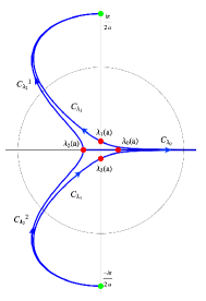
Figure 4: Contours (blue lines) and saddle points (red dots) of $\psi_{1}(\rho)$ and $\psi_{2}(\rho)$ in the $g(x)=\frac{\tan(x)}{x}$ case. The green dots are poles where the contours end.

In this appendix, we consider the contours $C_{>}$ and $C_{<}$ in the $g(x)=\frac{\tan(x)}{x}$ case. In this case, we have four regular saddle points:

$$\lambda_{k}(a)=\frac{\text{arctanh}{\left(e^{i\pi k/2}a\right)}}{a}\text{, for }k=0,1,2,3.$$ (156)

Note that $f_{\pm}(s)$ both have poles at $s=\pm\frac{i\pi}{2a}$. The endpoints of a contour are at either infinity or singularities. It turns out that in the $g(x)=\frac{\tan(x)}{x}$ case, the contours $C_{>}$ and $C_{<}$ both start from and terminate at poles $s=\pm\frac{i\pi}{2a}$. Following the conventions adopted in section II, we plot the contours $C_{>}$ and $C_{<}$ in FIG. 4, where the green dots are poles. The circle $C_{R}$ is also plotted in FIG. 4.

References

- (1) T. V. Fityo, I. O. Vakarchuk and V. M. Tkachuk, “WKB approximation in deformed space with minimal length,” J. Phys. A 39, no. 2, 379 (2006). doi:10.1088/0305-4470/39/2/0088
- (2) G. Blado, T. Prescott, J. Jennings, J. Ceyanes and R. Sepulveda, “Effects of the Generalized Uncertainty Principle on Quantum Tunneling,” Eur. J. Phys. 37, 025401 (2016) doi:10.1088/0143-0807/37/2/025401 [arXiv:1509.07359 [quant-ph]].
- (3) X. Guo, B. Lv, J. Tao and P. Wang, “Quantum Tunneling In Deformed Quantum Mechanics with Minimal Length,” arXiv:1609.06944 [gr-qc].
- (4) J. Tao, P. Wang and H. Yang, “Homogeneous Field and WKB Approximation In Deformed Quantum Mechanics with Minimal Length,” Adv. High Energy Phys. 2015, 718359 (2015) doi:10.1155/2015/718359 [arXiv:1211.5650 [hep-th]].
- (5) M. Eune and W. Kim, “Lifshitz scalar, brick wall method, and GUP in Horava-Lifshitz Gravity,” Phys. Rev. D 82, 124048 (2010) doi:10.1103/PhysRevD.82.124048 [arXiv:1007.1824 [hep-th]].
- (6) P. Wang, H. Yang and S. Ying, “Black Hole Radiation with Modified Dispersion Relation in Tunneling Paradigm: Free-fall Frame,” Eur. Phys. J. C 76, no. 1, 27 (2016) doi:10.1140/epjc/s10052-015-3858-y [arXiv:1505.04568 [gr-qc]].
- (7) P. Wang, H. Yang and S. Ying, “Minimal length effects on entanglement entropy of spherically symmetric black holes in the brick wall model,” Class. Quant. Grav. 33, no. 2, 025007 (2016) doi:10.1088/0264-9381/33/2/025007 [arXiv:1502.00204 [gr-qc]].
- (8) J. Z. Simon, “Higher Derivative Lagrangians, Nonlocality, Problems and Solutions,” Phys. Rev. D 41, 3720 (1990). doi:10.1103/PhysRevD.41.3720
- (9) C. L. Ching and R. Parwani, “Scattering and Bound States of a Deformed Quantum Mechanics,” arXiv:1207.1519 [hep-th].
- (10) M. Maggiore, “The Algebraic structure of the generalized uncertainty principle,” Phys. Lett. B 319, 83 (1993) doi:10.1016/0370-2693(93)90785-G [hep-th/9309034].
- (11) A. Kempf, G. Mangano and R. B. Mann, “Hilbert space representation of the minimal length uncertainty relation,” Phys. Rev. D 52, 1108 (1995) doi:10.1103/PhysRevD.52.1108 [hep-th/9412167].
- (12) P. K. Townsend, “Small Scale Structure of Space-Time as the Origin of the Gravitational Constant,” Phys. Rev. D 15, 2795 (1977). doi:10.1103/PhysRevD.15.2795
- (13) D. Amati, M. Ciafaloni and G. Veneziano, “Can Space-Time Be Probed Below the String Size?,” Phys. Lett. B 216, 41 (1989). doi:10.1016/0370-2693(89)91366-X
- (14) K. Konishi, G. Paffuti and P. Provero, “Minimum Physical Length and the Generalized Uncertainty Principle in String Theory,” Phys. Lett. B 234, 276 (1990). doi:10.1016/0370-2693(90)91927-4
- (15) L. N. Chang, D. Minic, N. Okamura and T. Takeuchi, “The Effect of the minimal length uncertainty relation on the density of states and the cosmological constant problem,” Phys. Rev. D 65, 125028 (2002) doi:10.1103/PhysRevD.65.125028 [hep-th/0201017].
- (16) F. Brau, “Minimal length uncertainty relation and hydrogen atom,” J. Phys. A 32, 7691 (1999) doi:10.1088/0305-4470/32/44/308 [quant-ph/9905033].
- (17) S. Das and E. C. Vagenas, “Universality of Quantum Gravity Corrections,” Phys. Rev. Lett. 101, 221301 (2008) doi:10.1103/PhysRevLett.101.221301 [arXiv:0810.5333 [hep-th]].
- (18) S. Hossenfelder, M. Bleicher, S. Hofmann, J. Ruppert, S. Scherer and H. Stoecker, “Collider signatures in the Planck regime,” Phys. Lett. B 575, 85 (2003) doi:10.1016/j.physletb.2003.09.040 [hep-th/0305262].
- (19) A. F. Ali, S. Das and E. C. Vagenas, “Discreteness of Space from the Generalized Uncertainty Principle,” Phys. Lett. B 678, 497 (2009) doi:10.1016/j.physletb.2009.06.061 [arXiv:0906.5396 [hep-th]].
- (20) X. Li, “Black hole entropy without brick walls,” Phys. Lett. B 540, 9 (2002) doi:10.1016/S0370-2693(02)02123-8 [gr-qc/0204029].
- (21) F. Brau and F. Buisseret, “Minimal Length Uncertainty Relation and gravitational quantum well,” Phys. Rev. D 74, 036002 (2006) doi:10.1103/PhysRevD.74.036002 [hep-th/0605183].
- (22) F. Scardigli, “Generalized uncertainty principle in quantum gravity from micro - black hole Gedanken experiment,” Phys. Lett. B 452, 39 (1999) doi:10.1016/S0370-2693(99)00167-7 [hep-th/9904025].
- (23) F. Scardigli and R. Casadio, “Gravitational tests of the Generalized Uncertainty Principle,” Eur. Phys. J. C 75, no. 9, 425 (2015) doi:10.1140/epjc/s10052-015-3635-y [arXiv:1407.0113 [hep-th]].
- (24) D. Chen, H. Wu, H. Yang and S. Yang, “Effects of quantum gravity on black holes, Int. J. Mod. Phys. A 29, no. 26, 1430054 (2014) doi:10.1142/S0217751X14300543 [arXiv:1410.5071 [gr-qc]].
- (25) S. Hossenfelder, “Minimal Length Scale Scenarios for Quantum Gravity,” Living Rev. Rel. 16, 2 (2013) doi:10.12942/lrr-2013-2 [arXiv:1203.6191 [gr-qc]].
- (26) G. Amelino-Camelia, “Introduction to quantum-gravity phenomenology,” Lect. Notes Phys. 669, 59 (2005) [gr-qc/0412136].
- (27) G. Amelino-Camelia, J. R. Ellis, N. E. Mavromatos, D. V. Nanopoulos and S. Sarkar, “Tests of quantum gravity from observations of gamma-ray bursts,” Nature 393, 763 (1998) doi:10.1038/31647 [astro-ph/9712103].
- (28) L. J. Garay, “Space-time foam as a quantum thermal bath,” Phys. Rev. Lett. 80, 2508 (1998) doi:10.1103/PhysRevLett.80.2508 [gr-qc/9801024].
- (29) G. Amelino-Camelia, “Doubly special relativity,” Nature 418, 34 (2002) doi:10.1038/418034a [gr-qc/0207049].
- (30) J. Magueijo and L. Smolin, “Generalized Lorentz invariance with an invariant energy scale,” Phys. Rev. D 67, 044017 (2003) doi:10.1103/PhysRevD.67.044017 [gr-qc/0207085].
- (31) D. Mattingly, “Modern tests of Lorentz invariance,” Living Rev. Rel. 8, 5 (2005) doi:10.12942/lrr-2005-5 [gr-qc/0502097].
- (32) S. Liberati, “Tests of Lorentz invariance: a 2013 update,” Class. Quant. Grav. 30, 133001 (2013) doi:10.1088/0264-9381/30/13/133001 [arXiv:1304.5795 [gr-qc]].
- (33) D. Colladay and V. A. Kostelecky, “Lorentz violating extension of the standard model,” Phys. Rev. D 58, 116002 (1998) doi:10.1103/PhysRevD.58.116002 [hep-ph/9809521].
- (34) S. R. Coleman and S. L. Glashow, “High-energy tests of Lorentz invariance,” Phys. Rev. D 59, 116008 (1999) doi:10.1103/PhysRevD.59.116008 [hep-ph/9812418].
- (35) G. Amelino-Camelia and T. Piran, “Planck scale deformation of Lorentz symmetry as a solution to the UHECR and the TeV gamma paradoxes,” Phys. Rev. D 64, 036005 (2001) doi:10.1103/PhysRevD.64.036005 [astro-ph/0008107].
- (36) T. Jacobson, S. Liberati and D. Mattingly, “TeV astrophysics constraints on Planck scale Lorentz violation,” Phys. Rev. D 66, 081302 (2002) doi:10.1103/PhysRevD.66.081302 [hep-ph/0112207].
- (37) T. A. Jacobson, S. Liberati, D. Mattingly and F. W. Stecker, “New limits on Planck scale Lorentz violation in QED,” Phys. Rev. Lett. 93, 021101 (2004) doi:10.1103/PhysRevLett.93.021101 [astro-ph/0309681].
- (38) S. Corley and T. Jacobson, “Hawking spectrum and high frequency dispersion,” Phys. Rev. D 54, 1568 (1996) doi:10.1103/PhysRevD.54.1568 [hep-th/9601073].
- (39) T. G. Pavlopoulos, “Breakdown of Lorentz invariance,” Phys. Rev. 159, 1106 (1967). doi:10.1103/PhysRev.159.1106
- (40) P. Wang and H. Yang, “Black Hole Radiation with Modified Dispersion Relation in Tunneling Paradigm: Static Frame,” arXiv:1505.03045 [gr-qc].
- (41) L. N. Chang, D. Minic, N. Okamura and T. Takeuchi, “Exact solution of the harmonic oscillator in arbitrary dimensions with minimal length uncertainty relations,” Phys. Rev. D 65, 125027 (2002) doi:10.1103/PhysRevD.65.125027 [hep-th/0111181].
- (42) J. S. Schwinger, “On gauge invariance and vacuum polarization,” Phys. Rev. 82, 664 (1951).
- (43) W. G. Unruh, “Notes on black hole evaporation,” Phys. Rev. D 14, 870 (1976). doi:10.1103/PhysRevD.14.870
- (44) R. A. Konoplya and A. Zhidenko, “Quasinormal modes of black holes: From astrophysics to string theory,” Rev. Mod. Phys. 83, 793 (2011) doi:10.1103/RevModPhys.83.793 [arXiv:1102.4014 [gr-qc]].
- (45) V. Ferrari and B. Mashhoon, “New approach to the quasinormal modes of a black hole,” Phys. Rev. D 30, 295 (1984). doi:10.1103/PhysRevD.30.295
- (46) H. P. Nollert, “TOPICAL REVIEW: Quasinormal modes: the characteristic ‘sound’ of black holes and neutron stars,” Class. Quant. Grav. 16, R159 (1999). doi:10.1088/0264-9381/16/12/201
- (47) S. Hod, “Bohr’s correspondence principle and the area spectrum of quantum black holes,” Phys. Rev. Lett. 81, 4293 (1998) doi:10.1103/PhysRevLett.81.4293 [gr-qc/9812002].
- (48) M. Maggiore, “The Physical interpretation of the spectrum of black hole quasinormal modes,” Phys. Rev. Lett. 100, 141301 (2008) doi:10.1103/PhysRevLett.100.141301 [arXiv:0711.3145 [gr-qc]].
- (49) J. D. Bekenstein, “The quantum mass spectrum of the Kerr black hole,” Lett. Nuovo Cim. 11, 467 (1974). doi:10.1007/BF02762768
- (50) P. Chen and R. J. Adler, “Black hole remnants and dark matter,” Nucl. Phys. Proc. Suppl. 124, 103 (2003) doi:10.1016/S0920-5632(03)02088-7 [gr-qc/0205106].
- (51) A. Vilenkin, “Quantum Creation of Universes,” Phys. Rev. D 30, 509 (1984). doi:10.1103/PhysRevD.30.509
- (52) A. Vilenkin, “Quantum Cosmology and the Initial State of the Universe,” Phys. Rev. D 37, 888 (1988). doi:10.1103/PhysRevD.37.888
- (53) B. R. Mu, P. Wang and H. T. Yang, “Minimal Length Effects on Schwinger Mechanism,” Commun. Theor. Phys. 63, no. 6, 715 (2015) doi:10.1088/0253-6102/63/6/715 [arXiv:1501.06020 [gr-qc]].
- (54) S. Haouat and K. Nouicer, “Influence of a Minimal Length on the Creation of Scalar Particles,” Phys. Rev. D 89, no. 10, 105030 (2014) doi:10.1103/PhysRevD.89.105030 [arXiv:1310.6966 [hep-th]].
- (55) G. Amelino-Camelia, M. Arzano, Y. Ling and G. Mandanici, “Black-hole thermodynamics with modified dispersion relations and generalized uncertainty principles,” Class. Quant. Grav. 23, 2585 (2006) doi:10.1088/0264-9381/23/7/022 [gr-qc/0506110].
- (56) J. D. Bekenstein, “Black holes and entropy,” Phys. Rev. D 7, 2333 (1973). doi:10.1103/PhysRevD.7.2333