Mathematical and numerical validation of the simplified spherical harmonics approach for time-dependent anisotropic-scattering transport problems in homogeneous media

Abstract

In this work, we extend the solid harmonics derivation, which was used by Ackroyd et al to derive the steady-state SP_N equations, to transient problems. The derivation expands the angular flux in ordinary surface harmonics but uses harmonic polynomials to generate additional surface spherical harmonic terms to be used in Galerkin projection. The derivation shows the equivalence between the SP_N and the P_N approximation. Also, we use the line source problem and McClarren’s “box” problem to demonstrate such equivalence numerically. Both problems were initially proposed for isotropic scattering, but here we add higher-order scattering moments to them. Results show that the difference between the SP_N and P_N scalar flux solution is at the roundoff level.

1 Introduction

The simplified spherical harmonics (SP_N) approximation was initially developed in the 1960s to reduce the number of degrees of freedom required to solve transport problems in multiple dimensions using moment-based methods such as the spherical harmonics (P_N) expansion [1, 2, 3]. Initially, the SP_N approximation was “derived” by Gelbard in an ad-hoc way by manipulating the P_N expansion from 1-D slab geometry to have a 3-D form. The theoretical study of the SP_N equations underwent a great awakening in the 1990s. Larsen, Morel and McGhee [4] made an asymptotic derivation of the SP_N equations and showed that the accuracy of the approximation is dependent upon the scattering ratio of the system. Subsequent works extended the asymptotic analysis to anisotropic or time-dependent problems [5, 6, 7, 8, 9]. However, the use of a Neumann series expansion to the unbounded streaming operator makes the asymptotic analysis a formal proof.

Another way to the SP_N equations follows the signposts of the solid harmonics. By generalizing the angular domain from $\mathbb{S}^{2}$ (i.e., the unit sphere) to $\mathbb{R}^{3}$ Ackroyd et al. used properties of solid harmonics to introduce additional harmonics, perform Galerkin projection, restrict the relaxed equations back to $\mathbb{S}^{2}$, and thereby derive the SP_N equations for steady-state, anisotropic scattering problems in homogeneous media [10, 11]. Later, Hanuš used solid harmonics in tensor form and derived the SP₃ equations for steady-state isotropic-scattering problems [12]; Chao was also able to use the solid harmonics approach to show that Pomraning’s angular flux trial space, which can lead to the SP_N equations [13], is a particular solution to the steady-state isotropic-scattering transport equation [14].

In this contribution, we would extend the solid harmonics derivation to time-dependent anisotropic-scattering homogeneous-media problems and numerically demonstrate the equivalence between SP_N and P_N equations. As such, we extend, albeit incrementally, the domain of applicability of the SP_N  equations to time-dependent, homogeneous problems with arbitrary scattering, a result that does not appear in the extant literature.

2 Solid Harmonics for Time-Dependent Transport Problems

As introduced in the previous section, the derivation below is based on solid harmonics which were also used by LABEL:\cite[cite]{[\@@bibref{Number}{missing}{}{}]}Ackroyd1999:IsotropicSHPn and [11]. Some of the properties of the solid harmonics that we use can be found in the papers, but for clarity in exposition are repeated herein.

2.1 Expansion of the Transport Equation

For monoenergetic neutron transport in homogeneous media, we begin with the equation [15, 16]

$$\frac{1}{v}\frac{\partial}{\partial t}\psi(\vec{r},\hat{\Omega},t)+\hat{\Omega}\cdot\nabla\psi(\vec{r},\hat{\Omega},t)+\sigma_{t}\psi(\vec{r},\hat{\Omega},t)=\oint_{\mathbb{S}^{2}}\psi(\vec{r},\hat{\Omega}^{\prime},t)\sigma_{s}(\hat{\Omega}\cdot\hat{\Omega}^{\prime})d\Omega^{\prime}+q(\vec{r},\hat{\Omega},t),$$ (1)

where the integration over $\mathbb{S}^{2}$ is often written as an integral over $4\pi$ in the transport literature.

The P_N approximation expands the angular flux and the anisotropic external source in terms of surface spherical harmonics

$$\psi(\vec{r},\hat{\Omega},t) =\sum_{l=0}^{\infty}\frac{2l+1}{4\pi}\psi_{l}(\vec{r},\hat{\Omega},t),$$ (2)

$$q(\vec{r},\hat{\Omega},t) =\sum_{l=0}^{\infty}\frac{2l+1}{4\pi}q_{l}(\vec{r},\hat{\Omega},t),$$ (3)

where

$$\psi_{l}(\vec{r},\hat{\Omega},t) =\sum_{m=-l}^{l}\psi_{l}^{m}(\vec{r},t)Y_{l}^{m}(\hat{\Omega}),$$ (4)

$$q_{l}(\vec{r},\hat{\Omega},t) =\sum_{m=-l}^{l}q_{l}^{m}(\vec{r},t)Y_{l}^{m}(\hat{\Omega}),$$ (5)

and $Y_{l}^{m}$ are the surface spherical harmonics [15], commonly referred to without the “surface” adjective.

The scattering cross-section can be expanded into

$$\sigma_{s}(\hat{\Omega}\cdot\hat{\Omega}^{\prime})=\sum_{l=0}^{\infty}\frac{2l+1}{4\pi}\sigma_{sl}\sum_{m=-l}^{l}Y_{l}^{m}(\hat{\Omega})Y_{l}^{m}(\hat{\Omega}^{\prime}),$$ (6)

so that, by defining

$$\sigma_{l}:=\sigma_{t}-\sigma_{sl},$$ (7)

Equation (1), by orthogonality of surface spherical harmonics, is written as the sum over $l$-moments

$$\sum_{l=0}^{\infty}(2l+1)\left[\left(\frac{1}{v}\frac{\partial}{\partial t}+\hat{\Omega}\cdot\nabla+\sigma_{l}\right)\psi_{l}(\vec{r},\hat{\Omega},t)-q_{l}(\vec{r},\hat{\Omega},t)\right]=0.$$ (8)

2.2 Galerkin Projection

The next step is to split the streaming term $(2l+1)\hat{\Omega}\cdot\nabla\psi_{l}(\vec{r},\hat{\Omega},t)$ into harmonics of degree $l-1$ and $l+1$ respectively, and this is where solid harmonics come to play their role.

Harmonic polynomials, often referred to as solid harmonics, are polynomials that are solutions to the Laplace equation, and a surface spherical harmonic of degree $l$ is the restriction onto $\mathbb{S}^{2}$ of a homogeneous harmonic polynomial on $\mathbb{R}^{3}$ of degree $l$ whose collection is denoted as $\mathcal{H}_{l}(\mathbb{R}^{3})$[17]. For $\vec{\Omega}\in\mathbb{R}^{3}$, solid harmonics can be obtained by rescaling surface harmonics by a factor of the length of $\vec{\Omega}$ to the $l$th power, $\Omega^{l}$, and the process relaxes the restriction of the domain from $\mathbb{S}^{2}$ to $\mathbb{R}^{3}$. In other words, if $Y_{l}^{m}(\hat{\Omega})$ is a surface harmonic, then $\Omega^{l}Y_{l}^{m}(\vec{\Omega})$ is a solid harmonic. For convenience, when $p_{l}$ is a surface harmonic, we denote the associated solid harmonic as $\tilde{p}_{l}$.

Now we make the following definitions for $\vec{\Omega}\in\mathbb{R}^{3}$

$$\nabla_{\Omega}:=\left(\frac{\partial}{\partial\Omega_{x}},\frac{\partial}{\partial\Omega_{y}},\frac{\partial}{\partial\Omega_{z}}\right)^{\text{T}},$$ (9)

$$\mathcal{P}:=\nabla_{\Omega}\cdot\nabla,\qquad\mathcal{Q}:=\vec{\Omega}\cdot\nabla,$$ (10)

and rewrite the streaming term $(2l+1)\hat{\Omega}\cdot\nabla\psi_{l}(\vec{r},\hat{\Omega},t)$ as

$$(2l+1)\hat{\Omega}\cdot\nabla\psi_{l}(\vec{r},\hat{\Omega},t)=\left[(2l+1)\mathcal{Q}\tilde{\psi}_{l}-\Omega^{2}\mathcal{P}\tilde{\psi}_{l}+\mathcal{P}\tilde{\psi}_{l}\right]_{\Omega=1}(\vec{r},\hat{\Omega},t),$$ (11)

where the subscript $\Omega=1$ denotes that the term inside brackets is restricted to the unit sphere.

It is proved in Reference [10] and shown in A that the term $\left[(2l+1)\mathcal{Q}\tilde{\psi}_{l}-\Omega^{2}\mathcal{P}\tilde{\psi}_{l}\right]$ is a solid harmonic of degree $l+1$ and $\mathcal{P}\tilde{\psi}_{l}$ is a solid harmonic of degree $l-1$. Ergo, when restricted back to $\mathbb{S}^{2}$, we get surface harmonics of degree $l-1$ and $l+1$.

Therefore, with Galerkin projection applied to Equation (8), we get

$$\left[(2n+1)\left(\frac{1}{v}\frac{\partial}{\partial t}+\sigma_{n}\right)\tilde{\psi}_{n}+\left((2n-1)\mathcal{Q}-\Omega^{2}\mathcal{P}\right)\tilde{\psi}_{n-1}+\mathcal{P}\tilde{\psi}_{n+1}-(2n+1)\tilde{q}_{n}\right]_{\Omega=1}=0.$$ (12)

To proceed, we will define two more operators:

$$\mathcal{F}\psi_{n}(\vec{r},\hat{\Omega},t):=\left[\left((2n+1)\mathcal{Q}-\Omega^{2}\mathcal{P}\right)\tilde{\psi}_{n}\right]_{\Omega=1}(\vec{r},\hat{\Omega},t),$$ (13)

and

$$\mathcal{G}\psi_{n}(\vec{r},\hat{\Omega},t):=\left[\mathcal{P}\tilde{\psi}_{n}\right]_{\Omega=1}(\vec{r},\hat{\Omega},t).$$ (14)

With these definitions Eq. (12) becomes

$$(2n+1)\left(\frac{1}{v}\frac{\partial}{\partial t}+\sigma_{n}\right)\psi_{n}(\vec{r},\hat{\Omega},t)+\mathcal{F}\psi_{n-1}(\vec{r},\hat{\Omega},t)+\mathcal{G}\psi_{n+1}(\vec{r},\hat{\Omega},t)=(2n+1)q_{n}(\vec{r},\hat{\Omega},t).$$ (15)

It is this form of the moment equations that we will manipulate to derive time-dependent SP_N equations.

2.3 Derivation of the SP_N Equations

To further simplify Equation (15), two useful identities from Reference [10] would be used

$$\left(\mathcal{P}\mathcal{Q}-\mathcal{Q}\mathcal{P}-\nabla^{2}\right)\tilde{\psi}_{n}=0,$$ (16)

$$\mathcal{P}\Omega^{2}\tilde{\psi}_{n}=(\Omega^{2}\mathcal{P}+2\mathcal{Q})\tilde{\psi}_{n}.$$ (17)

The two identities can be demonstrated using the definition of the underlying operators. Together, Eqs. (16) and (17) imply

$$\mathcal{P}^{n+1}\left[(2n+1)\mathcal{Q}-\Omega^{2}\mathcal{P}\right]\tilde{\psi}_{n}=(n+1)^{2}\nabla^{2}\mathcal{P}^{n}\tilde{\psi}_{n},$$ (18)

as shown in B. From these we can use the definition in Eq. (14) to obtain

$$\mathcal{G}^{n}\mathcal{F}\psi_{n-1}=n^{2}\nabla^{2}\mathcal{G}^{n-1}\psi_{n-1}.$$ (19)

Therefore, applying $\mathcal{G}$ $n$ times to Equation (15) yields

$$(2n+1)\frac{1}{v}\frac{\partial}{\partial t}\mathcal{G}^{n}\psi_{n}+(2n+1)\sigma_{n}\mathcal{G}^{n}\psi_{n}+n^{2}\nabla^{2}\mathcal{G}^{n-1}\psi_{n-1}+\mathcal{G}^{n+1}\psi_{n+1}=(2n+1)\mathcal{G}^{n}q_{n}.$$ (20)

Notice that $\mathcal{G}^{n}\psi_{n}$ and $\mathcal{G}^{n}q_{n}$ are surface harmonics of degree 0 and thus have no angular dependence, and that the inverse Laplace operator is well-defined in an infinite-medium problem. Using these facts, we can make the following substitution

$$F_{n}(\vec{r})=\frac{1}{n!}\nabla^{-2\lceil\frac{n}{2}\rceil}\mathcal{G}^{n}\psi_{n},$$ (21)

$$G_{n}(\vec{r})=\frac{1}{n!}\nabla^{-2\lceil\frac{n}{2}\rceil}\mathcal{G}^{n}q_{n}.$$ (22)

To these definitions we can relate the SP_N unknowns as, for $n$ a non-negative integer,

$$\phi_{2n}=F_{2n},\qquad\vec{\phi}_{2n+1}=\nabla F_{2n+1},$$ (23)

and write the source as

$$Q_{2n}=G_{2n},\qquad\vec{Q}_{2n+1}=\nabla G_{2n+1}.$$ (24)

These definitions will eventually lead us to the SP_N equations

$$\frac{1}{v}\frac{\partial}{\partial t}\phi_{n}+\sigma_{n}\phi_{n}+\frac{n}{2n+1}\nabla\cdot\vec{\phi}_{n-1}+\frac{n+1}{2n+1}\nabla\cdot\vec{\phi}_{n+1}=Q_{n}\ \ \ (n\text{ even}),$$ (25)

$$\frac{1}{v}\frac{\partial}{\partial t}\vec{\phi}_{n}+\sigma_{n}\vec{\phi}_{n}+\frac{n}{2n+1}\nabla\phi_{n-1}+\frac{n+1}{2n+1}\nabla\phi_{n+1}=\vec{Q}_{n}\ \ \ (n\text{ odd}).$$ (26)

Therefore, we have started with the time-dependent transport equation in a homogeneous medium and demonstrated that we can derive the SP_N equations using properties of the solid harmonics. Moreover, due to the way the derivation proceeded, a truncated P_N expansion should be equivalent to an SP_N solution truncated at the same level. Therefore, we expect that in a general problem, with homogeneous media, there to be an equivalence between the SP_N and P_N solutions.

3 Numerical Examples

In this section, we perform 2D simulations to demonstrate the equivalence between the SP_N and the P_N approximation for time-dependent, anisotropic scattering problems.

We solve the time-dependent SP_N and P_N equations under the implicit Euler scheme, so the problem is essentially a sequence of steady-state problems; the finite difference method is adopted so that all first-order derivatives are approximated by central differentiation; all moments are nodal values evaluated at grid points. For all the numerical examples below, periodic boundary conditions are enforced, the external source is isotropic and scattering is anisotropic.

3.1 An Anisotropic Box Problem

The first test problem comes from Reference [18], where McClarren used it to demonstrate the equivalence between steady-state P_N and SP_N , and Reference [19] refers to it as the “box” problem. The original problem has $\sigma_{t}=1\ cm^{-1}$ and isotropic scattering $\sigma_{s0}=0.1\ cm^{-1}$; here we add additional anisotropic scattering $\sigma_{s1}=0.1\ cm^{-1}=\sigma_{s2}=0.1\ cm^{-1}$ to show that such equivalence still holds for time-dependent anisotropic-scattering problems. The external source remains prescribed by

$$Q(x,y)=\begin{cases}1&1.75\leq x\leq 2.25,1.75\leq y\leq 2.25\\ 1&2.75\leq x\leq 3.25,1.5\leq y\leq 2.5\\ 1&1.75\leq x\leq 2.25,2.75\leq y\leq 3.25\\ 1&3.5\leq x\leq 4.25,3.5\leq y\leq 3.75\\ 0&\text{otherwise}\end{cases}$$ (27)

We perform the computation with $\Delta x=0.03\ \text{cm}$ and $\Delta t=0.03\ \text{s}$. The SP₃ scalar flux at $T=0.75\ \text{s}$ is compared with that at $T=1.5\ \text{s}$ in Figure 1; it can be seen that at $T=0.75\ \text{s}$, the problem is still in a transient state, thus we choose it as the final time of simulation.

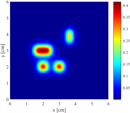
(a) $T=0.75\ \text{s}$

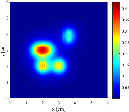
(b) $T=1.5\ \text{s}$

Figure 1: Comparison of SP₃ scalar flux at $T=0.75\ \text{s}$ and at $T=1.5\ \text{s}$

The scalar flux solutions for $N=1$ and $N=5$ at $T=0.75\ \text{s}$ are shown in Figure 2; we also plot the scalar flux along $y=x$ for $N=3$ and $N=7$ in Figure 3.

(a) SP₁

(b) P₁

(c) SP₅

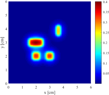
(d) P₅

Figure 2: Scalar flux computed at $T=0.75\ \text{s}$ for $N=1$ and $N=5$

(a) $N=3$

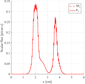
(b) $N=7$

Figure 3: Scalar flux computed at $T=0.75\ \text{s}$ along $y=x$ for $N=3$ and $N=7$

As can be seen from Figure 2-3, despite the existence of oscillations, the SP_N solutions agree with the P_N solutions. In fact, with $N$ ranging from 1 to 7, the $L^{\infty}$ norm of the deviation from SP_N solution to P_N solution does not exceed $1.6653\times 10^{-16}$, so we can claim that the two methods generate identical results.

3.2 An Anisotropic Line Source Problem

The line source (pulse) problem is a typical example to demonstrate the Gibbs phenomenon encountered by spectral methods, and it is also important as it is the Green’s function for problems with isotropic scattering and source. Here we modify the problem configuration to make the scattering anisotropic such that $\sigma_{t}=\sigma_{s0}=1\ cm^{-1}$, $\sigma_{s1}=0.5\ cm^{-1}$, $\sigma_{s2}=0.25\ cm^{-1}$ and $\sigma_{s3}=0.125\ cm^{-1}$, but the initial angular flux remains isotropic. To avoid the the singularity in the initial condition, the initial scalar flux $\phi(\vec{r},0)$, as suggested by Reference [19], is replaced by the distribution:

$$\phi(\vec{r},0)=\frac{1}{4\pi s}\exp\left(-\frac{r^{2}}{4s}\right)$$ (28)

where $s=3.2\times 10^{-4}$.

We perform numerical computation for $T=0.5\ \text{s}$ with $\Delta x=0.01\ \text{cm}$ and $\Delta t=0.005\ \text{s}$. Figure 4 shows that the solution of the anisotropic line source problem is different from that of the original line source problem, where the scattering is isotropic. The $L^{\infty}$ norm of the difference is 1.1810.

Figure 4: Comparison of SP₃ scalar flux of the original and the isotropic line source problem on a cut along the positive $x$-axis at $T=0.5\ \text{s}$

The scalar flux solutions for $N=3$ and $N=7$ are compared in Figure 5, where one can easily tell that the SP_N and P_N solutions are almost identical.

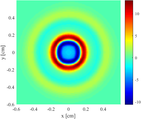
(a) SP₃

(b) P₃

(c) SP₇

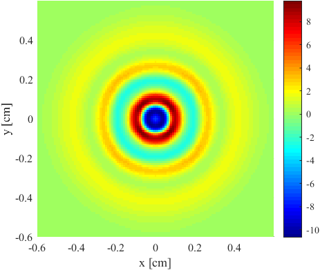
(d) P₇

Figure 5: Scalar flux for $N=3$ and 7 at $T=0.5\ \text{s}$

We also plot the scalar flux along the positive $x$-axis in Figure 6 for odd $N$ from 1 to 7. Though not shown in these figures, the SP_N solutions also agree with the P_N solutions for $N$=2, 4 and 6. For $N$ ranging from 1 to 7, the maximum of the $L^{\infty}$ norms of the SP_N and P_N scalar flux difference is $1.9540\times 10^{-14}$.

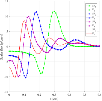
Figure 6: Scalar flux on a cut along the positive $x$-axis at $T=0.5\ \text{s}$

4 Discussions and Conclusions

With the use of harmonic polynomials, we derived the SP_N equations starting from the monoenergetic transport equation in homogeneous media. The derivation implies that we can expect the same scalar flux solution from either the SP_N or P_N approximation.

The theory is then followed by two numerical examples which are modified from the box problem and the line source problem to have anisotropic scattering. In both examples, the SP_N and P_N solutions match very well as the theoretical prediction.

We hope that the work can extend the research and application of the SP_N method. In fact, the study of the SP_N equations is far from over because the strongest theoretical results exist for homogenous, infinite media. The boundary and interface conditions the give SP_N-P_N equivalence in heterogeneous problems are a major, open problem. A less ambitious, but useful result, would be the development an algorithm that efficiently generates SP_N moments for anisotropic external source.

Appendix A Proof that the Two Terms in Equation (11) are Solid Harmonics

We will show how to prove that, if $p_{l}\in\mathcal{H}_{l}(\mathbb{R}^{3})$, then $\mathcal{P}p_{n}\in\mathcal{H}_{l-1}(\mathbb{R}^{3})$ and $\left[(2l+1)\mathcal{Q}-\Omega^{2}\mathcal{P}\right]p_{l}\in\mathcal{H}_{l+1}(\mathbb{R}^{3})$. The proof here is adopted from Reference [14] and Reference [10] has a different way. To prove that a function is a solid harmonic of degree $l$, it would be sufficient to show that it is a homogeneous polynomial of degree $l$ and that it is a solution to the Laplace equation.

First, let us consider the easy one, $\mathcal{P}p_{n}$. It is apparent that $\nabla_{\Omega}$ would result in a vector whose components are homogeneous polynomials of degree $l-1$, so $\nabla\cdot\nabla_{\Omega}p_{l}$ satisfies the first condition. To prove that $\nabla_{\Omega}^{2}\nabla\cdot\nabla_{\Omega}p_{l}=0$, one simply needs to commute the two operators and use the property that $\nabla_{\Omega}^{2}p_{l}=0$

$$\nabla_{\Omega}^{2}\nabla\cdot\nabla_{\Omega}p_{l}=\nabla\cdot\nabla_{\Omega}\nabla_{\Omega}^{2}p_{l}=0$$ (29)

So we have confirmed that $\mathcal{P}p_{l}\in\mathcal{H}_{l-1}(\mathbb{R}^{3})$.

Proving $\left[(2l+1)\mathcal{Q}-\Omega^{2}\mathcal{P}\right]p_{l}\in\mathcal{H}_{l+1}(\mathbb{R}^{3})$ takes slightly more work. Since both $\mathcal{Q}p_{l}$ and $\Omega^{2}\mathcal{P}p_{l}$ are homogeneous polynomials of degree $l+1$, the first condition is again easily met. The next is to prove

$$\nabla_{\Omega}^{2}\left((2l+1)\mathcal{Q}\right)p_{l}=\nabla_{\Omega}^{2}\Omega^{2}\mathcal{P}p_{l}$$ (30)

The way is to first prove, via simple vector algebra, that

$$\nabla_{\Omega}^{2}\Omega^{2}\mathcal{P}p_{l}=(6+4\vec{\Omega}\cdot\nabla_{\Omega}+\Omega^{2}\nabla_{\Omega}^{2})\mathcal{P}p_{l}=(6+4\vec{\Omega}\cdot\nabla_{\Omega})\mathcal{P}p_{l}$$ (31)

and that

$$\nabla_{\Omega}^{2}\mathcal{Q}p_{l}=(2\mathcal{P}+\mathcal{Q}\nabla_{\Omega}^{2})p_{l}=2\mathcal{P}p_{l}$$ (32)

By Euler’s homogeneous function theorem

$$\vec{\Omega}\cdot\nabla_{\Omega}\mathcal{P}p_{l}=(l-1)\mathcal{P}p_{l}$$ (33)

so Equation (31) yields

$$\nabla_{\Omega}^{2}\Omega^{2}\mathcal{P}p_{l}=2(2l+1)\mathcal{P}p_{l}$$ (34)

Equation (30) is a direct conclusion of Equation (32) and (34).

Appendix B Proof of Equation (18)

The objective here is to show that, with $p_{n}\in\mathcal{H}_{n}(\mathbb{R}^{3})$

$$\mathcal{P}^{n+1}\left[(2n+1)\mathcal{Q}-\Omega^{2}\mathcal{P}\right]p_{n}=(n+1)^{2}\nabla^{2}\mathcal{P}^{n}p_{n}$$ (35)

Reference [10] did this by proving

$$\mathcal{P}^{n+1}\mathcal{Q}p_{n}=(n+1)\nabla^{2}\mathcal{P}^{n}p_{n}$$ (36)

and

$$\mathcal{P}^{n+1}\Omega^{2}\mathcal{P}p_{n}=n(n+1)\nabla^{2}\mathcal{P}^{n}p_{n}$$ (37)

Both equations above can be proved using mathematical induction.

When $n=0$, the two equations become

$$\mathcal{P}\mathcal{Q}p_{0}=\nabla^{2}p_{0}$$ (38)

$$\mathcal{P}\Omega^{2}\mathcal{P}p_{0}=0$$ (39)

both of which are quite apparent.

Then, assuming that Equation (36) and (37) are valid for $n=k$, the corresponding equations for $k+1$ are

$$\mathcal{P}^{k+2}\mathcal{Q}p_{k+1}=(k+2)\nabla^{2}\mathcal{P}^{k+1}p_{k+1}$$ (40)

and

$$\mathcal{P}^{k+2}\Omega^{2}\mathcal{P}p_{k+1}=(k+1)(k+2)\nabla^{2}\mathcal{P}^{k+1}p_{k+1}$$ (41)

We will tackle the first equation first. By Equation (16)

$$\mathcal{P}^{k+2}\mathcal{Q}p_{k+1}=\mathcal{P}^{k+1}(\mathcal{Q}\mathcal{P}+\nabla^{2})p_{k+1}$$ (42)

By the equation for $n=k$

$$\mathcal{P}^{k+2}\mathcal{Q}p_{k+1}=\left((k+1)\nabla^{2}\mathcal{P}^{k+1}+\mathcal{P}^{k+1}\nabla^{2}\right)p_{k+1}=(k+2)\nabla^{2}\mathcal{P}^{k+1}p_{k+1}$$ (43)

So we have reached Equation (36), and will move on to prove Equation (41). By Equation (17)

$$\mathcal{P}^{k+2}\Omega^{2}\mathcal{P}p_{k+1}=\mathcal{P}^{k+1}(\Omega^{2}\mathcal{P}+2\mathcal{Q})\mathcal{P}p_{k+1}$$ (44)

By Equation (36) and Equation (37) for $n=k$

$$\mathcal{P}^{k+2}\Omega^{2}\mathcal{P}p_{k+1}=k(k+1)\nabla^{2}\mathcal{P}^{k+1}p_{k+1}+2(k+1)\nabla^{2}\mathcal{P}^{k+1}p_{k+1}$$ (45)

So we have also arrived at Equation (37) and Equation (35) is a direct conclusion following Equation (36) and (37).

References

- [1] E. Gelbard, Application of spherical harmonics method to reactor problems, Tech. Rep. WAPD-BT-20, Bettis Atomic Power Laboratory, Pittsburgh, PA (1960).
- [2] E. Gelbard, Simplified spherical harmonics equations and their use in shielding problems, Tech. Rep. WAPD-T-1182, Bettis Atomic Power Laboratory, Pittsburgh, PA (1961).
- [3] E. M. Gelbard, Applications of the simplified spherical harmonics equations in spherical geometry, Tech. Rep. WAPD-TM-294, Bettis Atomic Power Laboratory, Pittsburgh, PA (1962).
- [4] E. Larsen, J. Morel, J. McGhee, Asymptotic derivation of the simplified PN equations, in: Proceedings of Joint International Conference on Mathematical Methods and Supercomputing in Nuclear Applications, Portland, Oregon, 1993.
- [5] E. W. Larsen, J. Morel, J. M. McGhee, Asymptotic derivation of the multigroup P1 and simplified PN equations with anisotropic scattering, Nuclear science and engineering 123 (3) (1996) 328–342.
- [6] D. I. Tomašević, E. W. Larsen, The simplified P2 approximation, Nuclear science and engineering 122 (3) (1996) 309–325.
- [7] P. S. Brantley, E. W. Larsen, The simplified P3 approximation, Nuclear Science and Engineering 134 (1) (2000) 1–21.
- [8] M. Frank, A. Klar, E. W. Larsen, S. Yasuda, Time-dependent simplified PN approximation to the equations of radiative transfer, Journal of Computational Physics 226 (2) (2007) 2289–2305.
- [9] E. Olbrant, E. W. Larsen, M. Frank, B. Seibold, Asymptotic derivation and numerical investigation of time-dependent simplified PN equations, Journal of Computational Physics 238 (2013) 315–336.
- [10] R. Ackroyd, C. de Oliveira, A. Zolfaghari, A. Goddard, On a rigorous resolution of the transport equation into a system of diffusion-like equations, Progress in Nuclear Energy 35 (1) (1999) 1–64.
- [11] R. Ackroyd, C. De Oliveira, A. Zolfaghari, A. Goddard, On the exact resolution of the transport equation for an anisotropic scattering medium into a system of diffusive equations, Annals of Nuclear Energy 26 (8) (1999) 729–755.
- [12] M. Hanuš, Mathematical modeling of neutron transport, Ph.D. thesis, University of West Bohemia, Pilsen (2014).
- [13] G. Pomraning, Asymptotic and variational derivations of the simplified PN equations, Annals of Nuclear Energy 20 (9) (1993) 623–637.
- [14] Y.-A. Chao, A new and rigorous SPN theory for piecewise homogeneous regions, Annals of Nuclear Energy 96 (2016) 112–125.
- [15] G. I. Bell, S. Glasstone, Nuclear Reactor Theory, Robert E. Kreiger Publishing, Malabar, Florida, 1970.
- [16] R. G. McClarren, Spherical harmonics methods for thermal radiation transport, Ph.D. thesis, University of Michigan (2007).
- [17] S. Axler, P. Bourdon, R. Wade, Harmonic function theory, Vol. 137, Springer Science & Business Media, 2013.
- [18] R. G. McClarren, Theoretical aspects of the simplified PN equations, Transport Theory and Statistical Physics 39 (2-4) (2010) 73–109.
- [19] B. Seibold, M. Frank, StaRMAP—a second order staggered grid method for spherical harmonics moment equations of radiative transfer, ACM Transactions on Mathematical Software (TOMS) 41 (1) (2014) 4.