Precision measurement of antiproton to proton ratio with the Alpha Magnetic Spectrometer on the International Space Station

Abstract

A precision measurement by AMS of the antiproton-to-proton flux ratio in primary cosmic rays in the absolute rigidity range from 1 to 450 GV is presented based on $3.49\times 10^{5}$ antiproton events and $2.42\times 10^{9}$ proton events. Above $\sim 60$ GV the antiproton to proton flux ratio is consistent with being rigidity independent. A decreasing behaviour is expected for this ratio considering the traditional models for the secondary antiproton flux.

The measurement of the antiproton-to-proton flux ratio in primary Cosmic Rays (CR) is reported in the absolute rigidity range 1-450 GV. This measurement is based on 3.49 $\times 10^{5}$ antiproton events and 2.42 $\times 10^{9}$ proton events collected by the Alpha Magnetic Spectrometer, AMS ref:AMS2_first ; ref:AMS2_fraction ; ref:AMS2_epfluxes ; ref:AMS2_allele ; ref:AMS2_protons ; ref:AMS2_He ; ref:AMS2_pbar ; ref:AMS2_BC , on the International Space Station, ISS, from May 19, 2011 to May 26, 2015. The experimental data on antiprotons are limited ref:BESS ; ref:PAMELA because of their very low flux intensity, up to this measurement only a few$\times 10^{3}$ antiprotons were observed in the cosmic radiation. In the measurement of the antiproton component of the cosmic radiation a very large background is expected from the most abundant proton one: for each antiproton there are approximately $10^{4}$ protons, therefore, to measure the antiproton flux to 1$\%$ accuracy requires a separation power of $\sim 10^{6}$. The sensitivity of antiprotons to exotic CR sources, as dark matter annihilations, as well as to new phenomena in the propagation of CR in the galaxy is complementary to the sensitivity of the measurements of CR positrons. In particular, AMS has accurately measured the excess in the positron fraction to 500 GeV ref:AMS2_first ; ref:AMS2_fraction and this data generated many interesting theoretical models including collisions of dark matter particles, astrophysical sources, and collisions of CR (see e.g. ref:tom_last ; ref:tom_bay ; ref:tom_PHe ; ref:tom_unc ; ref:tom_2hal ; ref:tom_cfE ; ref:tom_posfra ; ref:donato ). Some of these models also include specific predictions for the antiproton flux and the antiproton-to-proton flux ratio in CR.

Detector. The description of the AMS detector is presented in ref:AMS2_first ; ref:AMS2_fraction ; ref:AMS2_epfluxes ; ref:AMS2_allele ; ref:AMS2_protons ; ref:AMS2_He ; ref:AMS2_pbar ; ref:AMS2_BC . All detector elements are used for particle identification in the present analysis: the silicon tracker TRK, the permanent magnet, the time of flight counters TOF, the anticoincidence counters ACC, the transition radiation detector TRD, the ring imaging Cherenkov detector RICH, and the electromagnetic calorimeter ECAL.

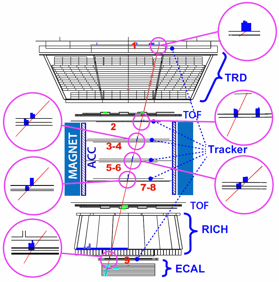
Figure 1: An event display in the bending plane of an antiproton. The red line indicates the reconstructed trajectory or track. The insets indicate the matching of the track to the pulse heights measured in each layer of the tracker. This downward-going $|Z|$ = 1 event is identified as an antiproton with R = -435 GV, $\Lambda_{TRD}$ = 0.908, and $\Lambda_{CC}$ = 0.983. See ref:AMS2_pbar for details.

The tracker, with its nine layers, is used to measure the rigidity R (momentum per unit of charge) of cosmic rays and to differentiate between positive and negative particles. The first layer (L1) is at the top of the detector, the second (L2) just above the magnet, six (L3 to L8) within the bore of the magnet, and the last (L9) just above the ECAL. L2 to L8 constitute the inner tracker. For $|Z|$ = 1 particles the maximum detectable rigidity, MDR, is 2 TV and the charge resolution is $\Delta$Z = 0.05. The TOF measures $|Z|$ and velocity with a resolution of $\Delta\beta/\beta^{2}=4\%$. The ACC has 0.99999 efficiency to reject particles entering the inner tracker from the side. The TRD separates $\bar{p}$ and p from $e^{-}$ and $e^{+}$ using the $\Lambda_{TRD}$ estimator constructed from the ratio of the log-likelihood probability of the $e^{\pm}$ hypothesis to that of the $\bar{p}$ or p hypothesis in each layer. Antiprotons and protons, which have $\Lambda_{TRD}$ $\sim 1$, are efficiently separated from electrons and positrons, which have $\Lambda_{TRD}$ $\sim$ 0.5. The RICH has a velocity resolution $\Delta\beta/\beta=0.1\%$ for $|Z|$ = 1 to ensure separation of $\bar{p}$ and p from light particles ($e^{\pm}$ and $\pi^{\pm}$) below 10 GV. The ECAL is used to separate $\bar{p}$ and p from $e^{-}$ and $e^{+}$ when the event can be measured by the ECAL. Antiprotons are separated from charge confused protons, that is, protons which are reconstructed in the tracker with negative rigidity due to the finite tracker resolution or due to interactions with the detector materials, by means of a charge confusion estimator $\Lambda_{CC}$ defined with a boosted decision tree technique BDT . The estimator combines information from the tracker such as the track $\chi^{2}$/d.o.f., rigidities reconstructed with different combinations of tracker layers, the number of hits in the vicinity of the track, and the charge measurements in the TOF and the tracker. With this method, antiprotons, which have $\Lambda_{CC}\sim$+1, are efficiently separated from charge confused protons, which have $\Lambda_{CC}\sim$-1. An example of a 435 GV antiproton crossing the AMS sub-detectors is given in Fig. 1.

Event selection and data samples. Over 65 billion CR events have been recorded in the first 48 months of AMS operations. Only events collected during normal detector operating conditions are used in this analysis. This includes the time periods when the AMS z axis is pointing within 40^o of the local zenith and when the ISS is not in the South Atlantic Anomaly. Data analysis is performed in 57 absolute rigidity bins. The same binning as in our proton flux measurement ref:AMS2_protons was chosen below 80.5 GV. Above 80.5 GV two to four proton bins are combined to ensure sufficient antiproton statistics. Events are selected requiring a track in the TRD and in the inner tracker and a measured velocity $\beta>$ 0.3 in the TOF corresponding to a downward-going particle. To maximize the number of selected events while maintaining an accurate rigidity measurement, the acceptance is increased by releasing the requirements on the external tracker layers, L1 and L9. Below 38.9 GV neither L1 nor L9 is required. From 38.9 to 147 GV either L1 or L9 is required. From 147 to 175 GV only L9 is required. Above 175 GV both L1 and L9 are required. In order to maximize the accuracy of the track reconstruction, the $\chi^{2}$/d.o.f. of the reconstructed track fit is required to be less than 10 both in the bending and nonbending projections. The dE/dx measurements in the TRD, the TOF, and the inner tracker must be consistent with $|Z|$ = 1. To select only primary CR, the measured rigidity is required to exceed the maximum geomagnetic cutoff by a factor of 1.2 for either positive or negative particles within the AMS field of view. The cutoff is calculated by backtracing using the most recent IGRF geomagnetic model. Events satisfying the selection criteria are classified into two categories: positive and negative rigidity events. A total of 2.42 $\times 10^{9}$ events with positive rigidity are selected as protons. They are 99.9$\%$ pure protons with almost no background. Deuterons are not distinguished from protons, their contribution decreases with rigidity: at 1 GV it is less than 2$\%$ and at 20 GV it is 0.6$\%$. The effective acceptance of this selection for protons is larger than in our proton flux publication ref:AMS2_protons . This is because there is no strict requirement that selected particles pass through the tracker layers L1 and L9 (see above) leading to a much larger field of view at low rigidities and, therefore, to a significant increase in the number of protons. The negative rigidity event category comprises both antiprotons and several background sources: electrons, light negative mesons ($\pi^{-}$ and a negligible amount of $K^{-}$) produced in the interactions of primary CR with the detector materials, and charge confused protons. The contributions of the different background sources vary with rigidity. For example, light negative mesons are present only at rigidities below 10 GV, whereas charge confusion becomes noticeable only at high rigidities. Electron background is present at all rigidities. The combination of information from the TRD, TOF, tracker, RICH, and ECAL enables the efficient separation of the antiproton signal events from these background sources using a template fitting technique. The number of observed antiproton signal events and its statistical error in the negative rigidity sample are determined in each bin by fitting signal and background templates to data by varying their normalization. As discussed below, the template variables used in the fit are constructed using information from the TOF, tracker, and TRD. The distribution of the variables for the template definition is the same for antiprotons and protons if they are both reconstructed with a correct charge-sign. This similarity has been verified with the Monte Carlo simulation and the antiproton and proton data of 2.97 $\leq|R|<$ 18.0 GV. Therefore, the signal template is always defined using the high-statistics proton data sample. Three overlapping rigidity regions with different types of template function are defined to maximize the accuracy of the analysis: low absolute rigidity region (1.00-4.02 GV), intermediate region (2.97-18.0 GV), and high absolute rigidity region (16.6-450 GV). In the overlapping rigidity bins, the results with the smallest error are selected. At low rigidities, a cut on the TRD estimator $\Lambda_{TRD}$ and the velocity measurement in the TOF are important to differentiate antiprotons from light particles ($e^{-}$ and $\pi^{-}$). Therefore, the mass distribution, calculated from the rigidity measurement in the inner tracker and the velocity measured by the TOF, is used to construct the templates and to differentiate between the antiproton signal and the background. The background $e^{-}$ and $\pi^{-}$ templates are defined from the data sample selected using information from the TRD, the RICH, and also the ECAL, when the event can be measured by the ECAL.

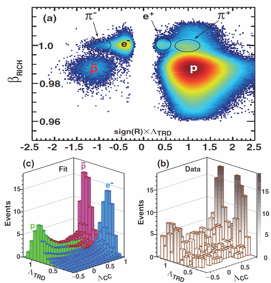
Figure 2: (a) Negative rigidity and positive rigidity data samples in the [$\beta_{RICH}$ - sign(R)$\times\Lambda_{TRD}$] plane for the absolute rigidity range 5.4-6.5 GV. The contributions of $\bar{p}$, p, $e^{+}$, $e^{-}$, $\pi^{+}$, and $\pi^{-}$ are clearly seen. The antiproton signal is well separated from the backgrounds. (b) For negative rigidity events, the distribution of data events in the ($\Lambda_{TRD}$ - $\Lambda_{CC}$) plane for the absolute rigidity bin 175-211 GV. (c) Fit with $\chi^{2}$/d.o.f. = 138/154 of the antiproton signal template (magenta), the electron background template (blue), and the charge confused proton background template (green) to the data in (b). See ref:AMS2_pbar for details.

At intermediate rigidities, $\Lambda_{TRD}$ and the velocity measured with the RICH $\beta_{RICH}$ are used to separate the antiproton signal from light particles ($e^{-}$ and $\pi^{-}$). As an example, Fig. 2.a shows that the antiproton signal and the background are well separated in the ($\beta_{RICH}$ - $\Lambda_{TRD}$) plane for the absolute rigidity range 5.4-6.5 GV. To determine the number of antiproton signal events, the $\pi^{-}$ background is removed by a rigidity dependent $\beta_{RICH}$ cut and the $\Lambda_{TRD}$ distribution is used to construct the templates and to differentiate between the $\bar{p}$ signal and $e^{-}$ background. The background template is defined from the $e^{-}$ data sample selected using ECAL. The Monte Carlo simulation matches the data for $e^{-}$ events inside the ECAL. The Monte Carlo simulation was then used to verify that the $e^{-}$ template shape outside the ECAL and inside the ECAL are identical. In the high rigidity region, the two-dimensional ($\Lambda_{TRD}$ - $\Lambda_{CC}$) distribution is used to determine the number of antiproton signal events. The lower bound of $\Lambda_{CC}$ is chosen for each bin to optimize the accuracy of the fit. For example, for $|R|>$ 175 GV, $\Lambda_{CC}$ $\geq$ -0.6. Variation of the lower bound is included in the systematic errors discussed below. To fit the data three template shapes are defined. The first two are for antiprotons and electrons with correctly reconstructed charge sign and the last one is for charge confused protons. The background templates (i.e., electrons and charge confused protons) are from the Monte Carlo simulation. The Monte Carlo simulation of the charge confusion was verified with the 400 GV proton test beam data. An example of the fit to the data is shown in Figs. 2.b and 2.c for the rigidity bin 175-211 GV. The distribution of data in the ($\Lambda_{TRD}$ - $\Lambda_{CC}$) plane is shown in Fig. 2.b and the fit results showing the signal and background distributions is highlighted in Fig. 2.c. The $\chi^{2}$ of the fit is 138 for 154 degrees of freedom. Overall, results for all 57 rigidity bins give a total of 3.49 $\times 10^{5}$ antiproton events in the data.

Analysis. The isotropic antiproton flux for the absolute rigidity bin $R_{i}$ of width $\Delta R_{i}$ is given by

$$\Phi_{i}^{\bar{p}}=\frac{N_{i}^{\bar{p}}}{A_{i}^{\bar{p}}T_{i}\Delta R_{i}}$$ (1)

where the rigidity is defined on top of the AMS, $N^{\bar{p}}_{i}$ is the number of antiprotons in the rigidity bin $i$ corrected with the rigidity resolution function ref:AMS2_pbar . $A^{\bar{p}}_{i}$ is the corresponding effective acceptance that includes geometric acceptance as well as the trigger and selection efficiency, and $T_{i}$ is the exposure time. Detector resolution effects cause migration of events $N^{\bar{p}}_{i}$ from rigidity bin $R_{i}$ to the measured rigidity bins $\tilde{R}_{j}$ resulting in the observed number of events $\tilde{N}_{i}^{\bar{p}}$. To account for this event migration, an iterative unfolding procedure is used to correct the number of observed events ref:AMS2_protons ; ref:AMS2_pbar . The same procedure is used to unfold the observed number of proton events. The ($\bar{p}/p$) flux ratio is defined for each absolute rigidity bin by:

$$\left(\frac{\bar{p}}{p}\right)_{i}=\frac{\Phi_{i}^{\bar{p}}}{\Phi_{i}^{p}}=\frac{\tilde{N}_{i}^{\bar{p}}}{\tilde{N}_{i}^{p}}\frac{\tilde{A}_{i}^{p}}{\tilde{A}_{i}^{\bar{p}}}$$ (2)

where $\tilde{A}_{i}^{p}/\tilde{A}_{i}^{\bar{p}}$ is the ratio of folded acceptances. We note that the $\tilde{A}_{i}^{p}/\tilde{A}_{i}^{\bar{p}}$ ratio decreases from 1.15 at 1 GV to 1.04 at 450 GV due to the varying difference of interaction cross sections for protons and antiprotons (and considering bin-to-bin event migration). With 3.49 $\times 10^{5}$ antiproton events, the accurate study of systematic errors is the key part of the present analysis, a detailed description can be found in ref:AMS2_pbar . Overall systematic error on the antiproton-to-proton flux ratio ranges from $\sim 8\%$ at 1 GV to $\sim 13\%$ in the last bin (259-450 GV) with a minimum of $\sim 2\%$ in the intermediate rigidity range ($\sim 30$ GV) ref:AMS2_pbar .

Results. The measured antiproton-to-proton flux ratio as a function of the absolute rigidity value at the top of the AMS is shown in Fig. 3.

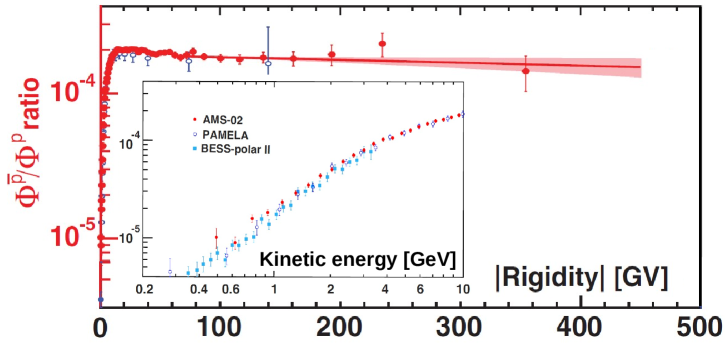
Figure 3: The measured ($\bar{p}/p$) flux ratio as a function of the absolute value of the rigidity from 1 to 450 GV. The PAMELA ref:PAMELA measurement is also shown (blue open circle). In the inset the ($\bar{p}/p$) flux ratio it is shown as a function of the kinetic energy up to 10 GeV. The kinetic energy is defined as $E_{K}=\sqrt{R^{2}+M^{2}}-M$ where M is the antiproton or proton mass. The BESS ref:BESS and PAMELA ref:PAMELA measurements are also shown. For the AMS data, the error bars are the quadratic sum of statistical and systematic errors. Horizontally, the data points are placed at the center of each bin. See ref:AMS2_pbar .

The AMS results, compared with earlier experiments, extend the rigidity range to 450 GV with increased precision. The inset Fig. 3 shows the low energy ($<$ 10 GeV) part of the measured flux ratio. The measured values of ($\bar{p}/p$) flux ratio, together with the statistical and systematic errors can be found in Table I of Supplemental Material of ref:AMS2_pbar and is stored online in the ASI/ASDC cosmic ray database ref:ASDC as well as all the other published results from the AMS experiment. The statistical errors are obtained from the fit errors on the signal, and both statistical and systematic error contributions to the total error in the flux ratio vary with rigidity. For 1.00 $\leq|R|<$ 1.33 GV the statistical error dominates, for 1.33 $\leq|R|<$ 1.71 GV the errors are comparable, for 1.71 $\leq|R|<$ 48.5 GV the systematic error dominates, for 48.5 $\leq|R|<$ 108 GV the errors are comparable, and for 108 $\leq|R|<$ 450 GV statistical error dominates. To minimize the systematic error for this flux ratio we have used the 2.42 $\times 10^{9}$ protons selected with the same acceptance, time period, and absolute rigidity range as the antiprotons. From 10 to 450 GV, the values of the proton flux are identical to 1$\%$ to those in our publication ref:AMS2_protons . As seen from Fig. 3 the ($\bar{p}/p$) flux ratio reaches a maximum at $\sim 20$ GV and above $\sim$60 GV appears to be rigidity independent. To estimate the lowest rigidity above which the ($\bar{p}/p$) ratio is rigidity independent, we use rigidity intervals with starting rigidities from 10 GV and increasing bin by bin. The ending rigidity for all intervals is fixed at 450 GV. Each interval is split into two sections with a boundary between the starting rigidity and 450 GV. Each of the two sections is fit with a constant and we obtain two mean values of the ($\bar{p}/p$) ratio. The lowest starting rigidity of the interval that gives consistent mean values at the 90$\%$ C.L. for any boundary defines the lowest limit. This yields 60.3 GV as the lowest rigidity above which the ($\bar{p}/p$) flux ratio is rigidity independent with a mean value of 1.81 $\pm$ 0.04 $\times 10^{-4}$. Further tests about the flatness of the measured ratio above $\sim 60$ GV are described in ref:AMS2_pbar . It is interesting to note that traditional models for the secondary antiproton flux are predicting a decreasing behaviour for the ($\bar{p}/p$) flux ratio (see e.g ref:donato ).

- (1) M. Aguilar et al., [AMS Collaboration] Phys. Rev. Lett. 110 (2013) 141102.
- (2) L. Accardo et al., [AMS Collaboration] Phys. Rev. Lett. 113 (2014) 121101.
- (3) M. Aguilar et al., [AMS Collaboration] Phys. Rev. Lett. 113 (2014) 121102.
- (4) M. Aguilar et al., [AMS Collaboration] Phys. Rev. Lett. 113 (2014) 221102.
- (5) M. Aguilar et al., [AMS Collaboration] Phys. Rev. Lett. 114 (2015) 171103.
- (6) M. Aguilar et al., [AMS Collaboration] Phys. Rev. Lett. 115 (2015) 211101.
- (7) M. Aguilar et al., [AMS Collaboration] Phys. Rev. Lett. 117 (2016) 091103.
- (8) M. Aguilar et al., [AMS Collaboration] Phys. Rev. Lett. 117 (2016) 231102.
- (9) K. Yoshimura et al., Phys. Rev. Lett. 75 (1995) 3792; S. Orito et al., Phys. Rev. Lett. 84 (2000) 1078; Y. Asaoka et al., Phys. Rev. Lett. 88 (2002) 051101; K. Abe et al., Phys. Lett. B 670 (2008) 103; 108 (2012) 051102; Astrophys. J. 822 (2016) 65.
- (10) O. Adriani et al., Phys. Rev. Lett. 102 (2009) 051101; 105 (2010) 121101; JETP Lett. 96 (2013) 621.
- (11) N. Tomassetti and J. Feng, Astrophys. J. 805 (2017) L26.
- (12) J. Feng et al., Phys. Rev. D94 (2016) 123007.
- (13) N. Tomassetti, Astrophys. J. 815 (2015) L1.
- (14) N. Tomassetti, Phys. Rev. C92 (2015) 045808.
- (15) N. Tomassetti, Phys. Rev. D92 (2015) 081301.
- (16) N. Tomassetti, Phys. Rev. D92 (2015) 063001.
- (17) N. Tomassetti et al., Astrophys. J. 803 (2015) L15.
- (18) F. Donato et al., Phys. Rev. Lett. 102 (2009) 071301.
- (19) B. P. Roe et al., Nucl. Instrum. Methods Phys. Res., Sect. A 543 (2005) 577.
- (20) ASI/ASDC cosmic ray database: http://tools.asdc.asi.it/cosmicRays.jsp