Anomalous transport and massive gravity theories

Abstract

We review the Kubo formulae relevant to study anomalous transport properties of relativistic fluids. We apply this formalism to perform a computation of the transport coefficients in a holographic massive gravity model including vorticity and external electromagnetic fields. We find an interesting phase in which the electric DC conductivity is negligible, while the anomalous conductivities turn out to be nonvanishing.

1 Introduction

Quantum anomalies are one of the most intriguing properties of relativistic field theories [1]. In the past few years it has been extensively studied the role played by quantum anomalies in the hydrodynamics of relativistic fluids. The hydrodynamical systems should obey the conservation laws of the energy-momentum tensor and spin one currents. In presence of anomalies the currents are no longer conserved, and this has important consequences in the constitutive relations for hydrodynamics. Two relevant phenomena induced by anomalies appear at first order in the hydrodynamical expansion: the chiral magnetic effect, which is the responsible for the generation of an electric current parallel to a magnetic field [2], and the chiral vortical effect, in which the electric current is induced by a vortex [3]. It is believed that these phenomena can produce observable effects in heavy ion physics [4], as well as in condensed matter systems [5]. It has been proposed in the literature several methods to compute the transport coefficients from a microscopic theory, either dissipative or non-dissipative, including kinetic theory [6], Kubo formulae [7, 8, 9], diagrammatic methods [10], fluid/gravity correspondence [11, 12, 13], and the partition function formalism [14, 15, 16, 17].

In addition to anomalies, there are other sources of non-conservation of the currents. In this context it is worth mentioning disorder as a very interesting property of some condensed matter systems [18]. Physical systems affected by disorder include real-world crystals with impurities, and the disorder phenomena can be manifested in the form of metal-insulator transitions [19]. From a quantum field theory perspective, disorder has to do with explicit breaking of translation invariance, so that it leads to momentum dissipation and the conservation of the energy-momentum tensor is modified. The study of disorder is particularly interesting in holography, as the AdS/CFT correspondence is a powerful tool that might help to establish some universal properties of these systems. Several holographic massive gravity models in AdS spacetimes have been recently proposed as a new and interesting approach to tackle this problem [20, 21]. It has been studied in these models some dissipative transport coefficients, like the DC electric conductivity, which turns out to be decreasing when disorder increases.

In this work we will review the Kubo formalism to study anomalous transport in hydrodynamics. In a second step, this formalism will be applied to study anomalous transport phenomena in a massive gravity model. We will contrast the result for the DC electric conductivity, with the one obtained for anomalous conductivities.

2 Hydrodynamics of relativistic fluids

Hydrodynamics is a useful approach to study many phenomena for physical systems out of equilibrium. It can be applied when the mean free path of particles is much shorter than the characteristic size of the system. The basic ingredients are the constitutive relations, which are expressions of the energy-momentum tensor and the charge currents in terms of fluid quantities [22],

$$\langle T^{\mu\nu}\rangle = (\varepsilon+P)u^{\mu}u^{\nu}+Pg^{\mu\nu}+\langle T^{\mu\nu}\rangle_{\textrm{\scriptsize diss \& anom}}\,,$$

$$\langle J^{\mu}\rangle = nu^{\mu}+\langle J^{\mu}\rangle_{\textrm{\scriptsize diss \& anom}}\,.$$

Here $\varepsilon$ is the energy density, $P$ the pressure, $n$ the charge density and $u^{\mu}$ the local fluid velocity. The equilibrium contributions are well known in the literature for many physical systems; however there are extra terms in the constitutive relations which lead to dissipative and anomalous effects. These extra contributions are in general difficult to compute, and the standard approach in hydrodynamics is to organize them in a derivative expansion, also called hydrodynamic expansion [12, 13, 23, 24]. In the Landau frame, defined as the one in which the energy flux vanishes at rest, the hydrodynamic expansion at first order in derivatives reads

$$\langle T^{\mu\nu}\rangle_{\textrm{\scriptsize diss \& anom}} = -\eta P^{\mu\alpha}P^{\nu\beta}\left(D_{\alpha}u_{\beta}\!+\!D_{\beta}u_{\alpha}\!-\!\frac{2}{3}g_{\alpha\beta}D^{\lambda}u_{\lambda}\right)-\zeta P^{\mu\nu}D^{\alpha}u_{\alpha}+\cdots\,,$$ (1)

$$\langle J^{\mu}\rangle_{\textrm{\scriptsize diss \& anom}}\!\!\!\! = \!\!\!\!-\sigma TP^{\mu\nu}D_{\nu}\left(\frac{\mu}{T}\right)+\sigma E^{\mu}+\sigma^{\cal B}B^{\mu}+\sigma^{\cal V}\omega^{\mu}+\cdots\,,$$ (2)

where $P^{\mu\nu}=g^{\mu\nu}+u^{\mu}u^{\nu}$ is the projector in the space orthogonal to the fluid velocity, $E^{\mu}=F^{\mu\nu}u_{\nu}$ and $B^{\mu}=\frac{1}{2}\epsilon^{\mu\nu\rho\lambda}u_{\nu}F_{\rho\lambda}$ are the electric and magnetic fields respectively, with the field strength of the gauge field defined as $F_{\mu\nu}=D_{\mu}A_{\nu}-D_{\nu}A_{\mu}$, and $\omega^{\mu}=\epsilon^{\mu\nu\rho\lambda}u_{\nu}D_{\rho}u_{\lambda}$ is the vorticity. The shear $\eta$ and bulk $\zeta$ viscosities play a prominent role in heavy ion experiments, as they are dissipative coefficients that are responsible for most of the entropy production of the quark gluon plasma during the collision, see e.g. [25]. The electric conductivity $\sigma$ is also dissipative, and its effects is to generate an electric current in the medium induced by an external electric field. Finally, the coefficients $\sigma^{\cal B}$ and $\sigma^{\cal V}$ are the so-called chiral magnetic [2] and chiral vortical [3] conductivities respectively, and they lead also to an electric current induced, either by an external magnetic field, or by a vortex in the fluid. As we will explain in Sec. 3, the coefficients $\sigma^{\cal B}$ and $\sigma^{\cal V}$ receive contributions from quantum anomalies, so that we will refer to them as anomalous conductivities.

In order to understand the (non)dissipative character of these transport coefficients, let us study their time reversal ${\cal T}$ properties. The second law of thermodynamics states that the entropy should increase with time, i.e.

$$\frac{\partial}{\partial t}s>0\,.$$ (3)

One can see from Eq. (3) that only ${\cal T}$-odd transport coefficients can contribute to the entropy production, while ${\cal T}$-even coefficients cannot. On the one hand the electric current $\vec{J}$ is ${\cal T}$-odd, while the electric field $\vec{E}$ is ${\cal T}$-even, and both the magnetic field $\vec{B}$ and vorticity $\vec{\omega}$ are ${\cal T}$-odd. Then, from a quick inspection of Eq. (2) one concludes that the electric conductivity $\sigma$ is ${\cal T}$-odd, while the chiral magnetic and vortical conductivities, $\sigma^{\cal B}$ and $\sigma^{\cal V}$, are ${\cal T}$-even. This explains the dissipative properties of $\sigma$, and the non-dissipative characters of $\sigma^{\cal B}$ and $\sigma^{\cal V}$. From a similar analysis of the parity ${\cal P}$ properties one finds that the chiral conductivities are related to ${\cal P}$-odd transport, see e.g. [23].

It is possible to observe non-dissipative effects also in the energy-momentum tensor under an appropriate choice of the frame (see Sec. 3.2), in particular the generation of an energy-flux induced by a magnetic field or by a vortex, i.e.

$$\langle T^{\mu\nu}\rangle_{\textrm{\scriptsize anom}} = \sigma_{\varepsilon}^{{\cal B}}(B^{\mu}u^{\nu}+B^{\nu}u^{\mu})+\sigma_{\varepsilon}^{{\cal V}}(\omega^{\mu}u^{\nu}+\omega^{\nu}u^{\mu})\,.$$ (4)

We will refer to $\sigma_{\varepsilon}^{{\cal B}}$ ($\sigma_{\varepsilon}^{{\cal V}}$) as chiral magnetic (vortical) conductivity of energy current. In the rest of this work we will study the transport coefficients $\sigma$, $\sigma^{\cal B}$, $\sigma^{\cal V}$, $\sigma_{\varepsilon}^{{\cal B}}$ and $\sigma_{\varepsilon}^{{\cal V}}$. We will be especially focused on the chiral conductivities.

3 Kubo Formulae

On the basis of linear response theory, hydrodynamic transport coefficients can be extracted from the long-wavelength and low-frequency limits of some retarded Green functions, leading to the so called Kubo formulae. The Kubo formula for the chiral magnetic conductivity was derived in [26], while the one for the chiral vortical conductivity was studied in [7]. They read, respectively,

$$\sigma^{\cal B}=\lim_{p_{c}\rightarrow 0}\frac{i}{2p_{c}}\sum_{a,b}\epsilon_{abc}\langle J^{a}J^{b}\rangle|_{\omega=0}\,,\quad\sigma^{\cal V}=\lim_{p_{c}\rightarrow 0}\frac{i}{2p_{c}}\sum_{a,b}\epsilon_{abc}\langle J^{a}T^{0b}\rangle|_{\omega=0}\,.$$ (5)

Similar Kubo formulae have been derived for the transport coefficients related to the generation of energy flux, in particular $\sigma_{\varepsilon}^{{\cal B}}\sim\epsilon_{abc}\langle T^{0a}J^{b}\rangle$ and $\sigma_{\varepsilon}^{{\cal V}}\sim\epsilon_{abc}\langle T^{0a}T^{0b}\rangle$, see [7, 27, 8, 9]. We will study in this section the result of the computation of Eq. (5) at weak and strong coupling.

3.1 Weak coupling results

Let us consider a theory of $N$ free chiral fermions transforming under a global symmetry group $G$ generated by matrices $(T_{A})^{f}\,{}_{g}$. The chemical potential for the fermion $\Psi^{f}$ is given by $\mu^{f}=\sum_{A}q_{A}^{f}\mu_{A}$, while the Cartan generator is $H_{A}=q^{f}_{A}\delta^{f}\,{}_{g}$ where $q^{f}_{A}$ are the charges. It has been performed in the literature the 1-loop computation of the chiral magnetic [26] and the chiral vortical [28] conductivities by using the Kubo formulae of Eq. (5). The results read, respectively,

$$(\sigma^{\cal B})_{AB}=\frac{1}{4\pi^{2}}d_{ABC}\mu^{C}\,,\qquad(\sigma^{\cal V})_{A}=\frac{1}{8\pi^{2}}\sum_{B,C}d_{ABC}\,\mu^{B}\,\mu^{C}+\frac{T^{2}}{24}b_{A}\,,$$ (6)

where the coefficients

$$d_{ABC}=\frac{1}{2}\left[\tr(T_{A}\{T_{B},T_{C}\})_{R}-\tr(T_{A}\{T_{B},T_{C}\})_{L}\right]\,,\qquad b_{A}=\tr\left(T_{A}\right)_{R}-\tr\left(T_{A}\right)_{L}\,,$$ (7)

are related to the trace of the generators of the symmetry group. The subscripts $R$, $L$ stand for the contributions of right-handed and left-handed fermions. One can easily identify $d_{ABC}$ with the group theoretic factor related to the axial anomaly, which typically appears in the computation of the anomalous triangle diagram corresponding to three non-abelian gauge fields coupled to a chiral fermion. On the other hand, the coefficient $b_{A}$ corresponds to the mixed gauge-gravitational anomaly [29], appearing in the anomalous triangle diagram with one non-abelian gauge field and two insertions of the energy-momentum tensor coupled to a chiral fermion. This means that the chiral magnetic and chiral vortical conductivities are induced by chiral anomalies, either the axial anomaly or the mixed gauge-gravitational anomaly.

Anomalies are also responsible for a non-vanishing value of the divergence of the currents, which in this case reads [30] 

$$D_{\mu}J_{A}^{\mu}=\epsilon^{\mu\nu\rho\lambda}\left(\frac{d_{ABC}}{32\pi^{2}}F^{B}_{\mu\nu}F^{C}_{\rho\lambda}+\frac{b_{A}}{768\pi^{2}}R^{\alpha}\,_{\beta\mu\nu}R^{\beta}\,_{\alpha\rho\lambda}\right)\,.$$ (8)

A clear consequence of Eq. (8) is that anomalies modify the hydrodynamic equations, due to the non-conservation of the currents. So it is obvious that they should affect the hydrodynamic expansion with new contributions not appearing in absence of anomalies. We have identified above these new contributions at first order in derivatives as $\sigma^{\cal B}$ and $\sigma^{\cal V}$ in Eq. (2). 

3.2 Strong coupling results

The Kubo formulae Eq. (5) have been computed in [27, 24, 32] at strong coupling within a Einstein-Maxwell model in 5 dim. In order to mimic the anomalous effects, the model is supplemented with pure gauge and mixed gauge-gravitational Chern-Simons terms. The action reads

$$S = \frac{1}{16\pi G}\int d^{5}x\sqrt{-g}\Bigg{[}R+12-\frac{1}{4}F_{MN}F^{MN}$$ (9)

$$+\epsilon^{MNPQR}A_{M}\left(\frac{\kappa}{3}F_{NP}F_{QR}+\lambda R^{A}\,_{BNP}R^{B}\,_{AQR}\right)\Bigg{]}+S_{GH}+S_{CSK}\,,$$

where $S_{GH}$ is the usual Gibbons-Hawking boundary term, and $S_{CSK}$ is an extra boundary contribution needed to reproduce the mixed gauge-gravitational anomaly at a general hypersurface. A computation of the current with this model leads to

$$\tilde{J}^{\mu}=\frac{\partial S}{\partial A_{\mu}}=-\frac{\sqrt{-\gamma}}{16\pi G}\left[F^{r\mu}+\frac{4}{3}\kappa\epsilon^{\mu\nu\rho\lambda}A_{\nu}F_{\rho\lambda}\right]_{\partial}\equiv J^{\mu}+K^{\mu}\,.$$ (10)

Note that $\tilde{J}^{\mu}$ is not gauge covariant, and we refer to it as consistent current. The covariant version of the current, denoted by $J^{\mu}$, is the usual one appearing in the constitutive relations. From Eq. (10), an on-shell computation of the divergence of the covariant current leads to the anomaly 

$$D_{\mu}J^{\mu}=-\frac{1}{16\pi G}\epsilon^{\mu\nu\rho\lambda}\left(\kappa{\hat{F}}_{\mu\nu}{\hat{F}}_{\rho\lambda}+\lambda{\hat{R}}^{\alpha}\,_{\beta\mu\nu}{\hat{R}}^{\beta}\,_{\alpha\rho\lambda}\right)\,.$$ (11)

Finally, from a comparison with Eq. (8) one can identify the parameters $\kappa$ and $\lambda$ as the axial anomaly and mixed gauge-gravitational anomaly coefficients, respectively.

The holographic computation of the transport coefficients with the Kubo formulae follows from the study of retarded propagators by using the AdS/CFT dictionary [33, 34]. In general lines, we split the metric and gauge field into a background and a linear perturbation

$$g_{MN}=g^{(0)}_{MN}+\epsilon\,h_{MN}\,,\qquad A_{M}=A_{M}^{(0)}+\epsilon\,a_{M}\,.$$ (12)

Inserting these fields in the action and expanding up to second order in $\epsilon$ one can obtain the second order action, and from there the desired propagators [35]. The equations of motion of the fluctuations should obey appropriate boundary conditions, in particular: i) regularity at the horizon; and ii) vanishing at the boundary, as the fluctuations cannot modify the boundary values, which are given by the background. There is some freedom in one of the boundary conditions which is related to the choice of frame. This corresponds to the particular definition of the local fluid velocity.

We show in Table 1 the values of the anomalous conductivities computed with the holographic model of Eq. (9), corresponding to a system which realizes a single $U_{A}(1)$ symmetry. We display the results in three different frames. $u^{\mu}$ can be taken to be proportional to: i) the energy flux $\langle T^{0i}\rangle=(\varepsilon+P)u^{i}$ (Landau frame), and ii) the charge current $\langle J^{i}\rangle=nu^{i}$ (Eckart frame). In addition, the laboratory rest frame is the natural frame in the field theory computation, see Sec. 3.1, and it seems to be related to the entropy current $\langle J^{i}_{S}\rangle_{\textrm{\scriptsize anom}}=0$, see e.g. [36].

Conductivities	Laboratory rest frame	Landau frame	Eckart frame
$\qquad(\sigma^{\cal B})_{\textrm{\tiny F}}$	$\sigma^{\cal B}=\frac{\mu}{4\pi^{2}}$	$\sigma^{\cal B}-\frac{n}{\varepsilon+P}\sigma_{\varepsilon}^{{\cal B}}$	$\qquad 0$
$\qquad(\sigma^{\cal V})_{\textrm{\tiny F}}$	$\sigma^{\cal V}=\frac{\mu^{2}}{8\pi^{2}}+\frac{T^{2}}{24}$	$\sigma^{\cal V}-\frac{n}{\varepsilon+P}\sigma_{\varepsilon}^{{\cal V}}$	$\qquad 0$
$\qquad(\sigma_{\varepsilon}^{{\cal B}})_{\textrm{\tiny F}}$	$\sigma_{\varepsilon}^{{\cal B}}=\sigma^{\cal V}$	$\qquad 0$	$\sigma_{\varepsilon}^{{\cal B}}-\frac{\varepsilon+P}{n}\sigma^{\cal B}$
$\qquad(\sigma_{\varepsilon}^{{\cal V}})_{\textrm{\tiny F}}$	$\sigma_{\varepsilon}^{{\cal V}}=\frac{\mu^{3}}{12\pi^{2}}+\frac{\mu T^{2}}{12}$	$\qquad 0$	$\sigma_{\varepsilon}^{{\cal V}}-\frac{\varepsilon+P}{n}\sigma^{\cal V}$

Table 1: Anomalous conductivities contributing to the constitutive relations, Eqs. (2) and (4), for a theory with a single chiral $U_{A}(1)$ symmetry. The result at weak and strong coupling agree.

Let us finally stress that the values of the anomalous conductivities at strong coupling coincide precisely with the ones obtained at weak coupling, and this a strong hint towards a non-renormalization theorem for the anomalous conductivities, see e.g. [28, 27, 32]. 

4 Transport properties in massive gravity

It has been recently studied in [20, 21] some minimal models for massive gravity in 4 dim. The momentum relaxation is described through the Stueckelberg mechanism with Goldstone modes corresponding to scalars $X^{I}$, which are related to spatial translations. In this section we will consider the model presented in [21]. We have explicitly checked that our conclusions are the same when considering the model of [20].

4.1 The model

In order to study anomalous transport in holographic massive gravity theories, one should consider the theory in odd dimensions, as only in these cases there is contribution from the chiral anomaly and we can introduce the corresponding Chern-Simons terms, see Eq. (9). We will consider the model of [21], and extend it to 5 dim. The action reads

$$S=\frac{1}{16\pi G}\int d^{5}x\sqrt{-g}\left[R+12-\frac{1}{2}\partial^{M}X^{I}\partial_{M}X^{I}-\frac{1}{4}F^{2}-\frac{\cal J}{4}\partial_{M}X^{I}\partial_{N}X^{I}F^{N}\,_{L}F^{LM}\right]\,,$$ (13)

with scalar fields $X^{I}=k\delta^{I}_{i}x^{i}$, where $i$ denotes spatial directions. Momentum relaxation is implemented by giving the scalar fields a vacuum expectation value. The term $\sim{\cal J}$ is a higher derivative coupling between the charge and the scalar field. The parameter $k$ controls the degree of breaking of translational invariance, in particular when $k=0$ one recovers the massless gravity theory. The equations of motion for the fields $(\delta g^{MN},\delta A^{M},\delta X^{I})$ read

$$0 = G_{MN}-6g_{MN}+\frac{1}{2}F_{M}\,{}^{L}F_{LN}-\frac{1}{8}g_{MN}F^{2}-\frac{1}{2}\partial_{M}X^{I}\partial_{N}X^{I}+\frac{1}{4}g_{MN}(\partial_{L}X^{I})(\partial^{L}X^{I})$$ (14)

$$-\frac{\cal J}{4}\left(\tilde{X}.F.F+F.\tilde{X}.F+F.F\tilde{X}\right)_{MN}+\frac{\cal J}{8}g_{MN}\mathrm{tr}(\tilde{X}.F.F)\,,$$

$$0 = \nabla_{N}F^{NM}+\frac{\cal J}{2}\nabla_{L}(\tilde{X}.F)^{ML}-\frac{\cal J}{2}\nabla_{L}(\tilde{X}.F)^{LM}\,,$$ (15)

$$0 = \Box X^{I}+\frac{{\cal J}}{2}\nabla_{M}(\partial_{N}X^{I}F^{N}\,_{L}F^{LM})\,,$$ (16)

where $\tilde{X}_{MN}\equiv\partial_{M}X^{I}\partial_{N}X^{I}$, and the products are $\tilde{X}.F.F=\partial_{M}X^{I}\partial_{N}X^{I}F^{N}\,_{L}F^{LM}$, etc. These equations can be solved with the black-brane ansatz:

$$ds^{2}=-fdt^{2}+\frac{dr^{2}}{f}+r^{2}d\vec{x}^{2}\,,\qquad A=A_{t}\,dt\,.$$ (17)

We find the following solution:

$$f=r^{2}-\frac{M}{r^{2}}+\frac{\rho^{2}}{3r^{4}}+\frac{k^{2}}{2}\,,\qquad A_{t}=\mu-\frac{\rho}{r^{2}}\,,$$ (18)

and the temperature and chemical potential can be related to the mass $M$ and charge $\rho$ of the black hole as

$$T=\frac{1}{2\pi r_{h}}\left(\frac{2M}{r_{h}^{2}}-\mu^{2}-\frac{k^{2}}{2}\right)\,,\qquad\mu r_{h}^{2}=\rho\,,$$ (19)

where $r_{h}$ is the black hole horizon corresponding to the largest solution of $f=0$.

4.2 Electric DC conductivity

As shown in Eq. (2), the electric conductivity measures the electric current $J^{\mu}$ induced by an electric field $E^{\mu}$. There are several methods to compute the DC conductivity in holography, but one of the most straightforward is the one proposed in [41]. We consider the following ansatz for the fluctuations in the gauge field and the metric:

$$A_{x}=\epsilon(Et+a_{x}(r))\,,\qquad g_{tx}=r^{2}(1+\epsilon h_{tx}(r))\,,\qquad g_{rx}=r^{2}(1+\epsilon h_{rx}(r))\,,$$ (20)

and work to first order in $\epsilon$. The fluctuation equations can be written now as

$$0= \frac{k^{2}}{2}\left(1-\frac{2{\cal J}\rho^{2}}{r^{6}}\right)h_{rx}-\left(1-\frac{{\cal J}k^{2}}{2r^{2}}\right)\frac{E\rho}{fr^{3}}\,,$$ (21)

$$r^{8}f(h_{tx}^{\prime\prime}+\frac{5}{r}h_{tx}^{\prime}) =k^{2}(r^{6}+2{\cal J}\rho^{2})-\rho(2r^{2}-k^{2}{\cal J}^{2})(rfa_{x}^{\prime})\,,$$ (22)

$$0= \left[\left(1-\frac{{\cal J}k^{2}}{2r^{2}}\right)rfa_{x}^{\prime}+\left(2-\frac{{\cal J}k^{2}}{r^{2}}\right)\rho h_{tx}\right]^{\prime}\,.$$ (23)

The DC conductivity can be obtained from a solution of these equations with appropriate boundary conditions at the horizon and the boundary, as explained in Sec. 3.2. At this point we will skip the technical details, that will be presented in [42]. The final result for the DC conductivity reads

$$\sigma_{DC}=\frac{J_{x}}{E}=r_{h}\left(1-\frac{{\cal J}k^{2}}{2r_{h}^{2}}\right)\left[1+\left(1-\frac{{\cal J}k^{2}}{2r_{h}^{2}}\right)\frac{4\mu^{2}}{k^{2}M(r_{h})}\right]\,,$$ (24)

with $M(r_{h})=1+\frac{2{\cal J}\rho^{2}}{r_{h}^{6}}$. This formula is the equivalent to the result presented in Eq. (3.15) of [21], but in 5 dim. We plot in Fig. 1 the value of the DC conductivity from Eq. (24) as a function of the parameter $k$ (left) and the temperature $T$ (right) for different values of the parameter ${\cal J}$. On the one hand, we observe that in the case ${\cal J}=0$, the conductivity is bounded from below, so that there is no insulating behavior without ${\cal J}$. More important is the fact that when ${\cal J}\neq 0$, there is a particular value $k_{*}=k({\cal J})$ at which the DC conductivity vanishes, so that the theory behaves as an insulator. This property is one of the main results of [20, 21] in 4 dim, and here we have reproduced it as well in 5 dim. Finally, we show in Fig. 2 the regime of parameters where the DC conductivity vanishes.

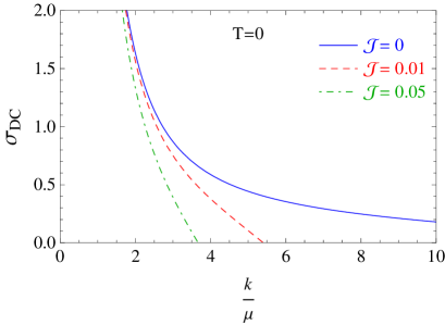
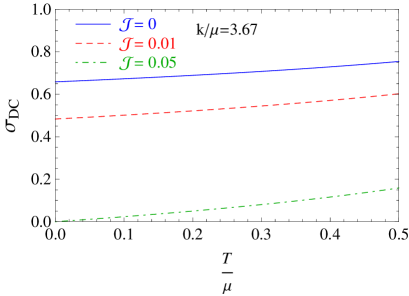
(A)	(B)

Figure 1: (A) DC conductivity at zero temperature as a function of $k$ (normalized to the chemical potential $\mu$). (B) DC conductivity (at fixed $k/\mu=3.67$) as a function of temperature (normalized to $\mu$). These results are obtained with Eq. (24) for different values of the parameter ${\cal J}$.

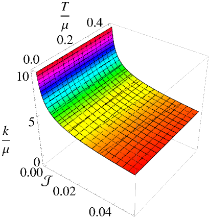
Figure 2: Region in the plane $({\cal J},T/\mu,k/\mu)$ where the DC conductivity of Eq. (24) vanishes.

4.3 Anomalous Transport

In Sec. 4.2 we have studied some dissipative properties of the 5 dim massive gravity model. In order to study non-dissipative transport coefficients, we should introduce anomalous effects in the theory. As we explained in Sec. 3, anomalies are mimicked in the gravity side through Chern-Simons terms. When extending the model of Eq. (13) with the Chern-Simons terms of Eq. (9), extra contributions appear in the equations of motion of the theory, in particular the term $-2\lambda\epsilon_{LPQR(M}\nabla_{B}\left(F^{PL}R^{B}\,_{N)}\,{}^{QR}\right)$ in the rhs of Eq. (14), and the terms $\epsilon^{MNPQR}(\kappa F_{NP}F_{QR}+\lambda R^{A}\,_{BNP}R^{B}\,_{AQR})$ in the rhs of Eq. (15). By using the following conventions

$$ds^{2}=\frac{du^{2}}{4u^{2}f(u)}+\frac{1}{u}\left(f(u)dt^{2}+2h_{ti}(u)e^{ipz}dtdx^{i}+d\vec{x}^{2}\right)\,,$$ (25)

where $i=x,y$, the fluctuation equations are

$$0 = (a_{i}^{\prime}f)^{\prime}-\rho h_{ti}^{\prime}-ip\epsilon_{ij}\left[4\kappa\rho a_{j}+\lambda\left(12u^{2}\rho^{2}+\frac{24}{u}(1-f)+5k^{2}\right)h_{tj}^{\prime}\right]\,,$$ (26)

$$0 = h_{ti}^{\prime\prime}-\frac{1}{u}h_{ti}^{\prime}-\frac{k^{2}}{4uf}h_{ti}-u\rho a_{i}^{\prime}+ip\lambda\epsilon_{ij}\left[\left(24(1-f)-12u^{3}\rho^{2}-5uk^{2}\right)a_{j}^{\prime}+\right.$$ (27)

$$+\left.\left(\frac{24}{u}(1-f)-32u^{2}\rho^{2}-6k^{2}\right)a_{j}-8\rho u(uh_{ti}^{\prime})^{\prime}\right]\,.$$

Finally, from the procedure of Sec. 3 we get the result for the anomalous conductivities: 

$$\sigma^{\cal B} = \lim_{p\to 0}\frac{i}{p}\langle J^{x}J^{y}\rangle=\kappa 4\mu\,,$$ (28)

$$\sigma^{\cal V} = \lim_{p\to 0}\frac{i}{p}\langle J^{x}T^{0y}\rangle=\kappa 2\mu^{2}+\lambda 16\pi^{2}T^{2}\,,$$ (29)

$$\sigma_{\varepsilon}^{\cal B} = \lim_{p\to 0}\frac{i}{p}\langle T^{0x}J^{y}\rangle=\kappa 2\mu^{2}+\lambda 16\pi^{2}T^{2}+\lambda 2k^{2}\,,$$ (30)

$$\sigma_{\varepsilon}^{\cal V} = \lim_{p\to 0}\frac{i}{p}\langle T^{0x}T^{0y}\rangle=\kappa\frac{4}{3}\mu^{3}+\lambda 32\pi^{2}T^{2}\mu\,.$$ (31)

Some remarks deserve to be mentioned at this point. On the one hand the chiral magnetic and vortical conductivities of charge currents, $\sigma^{\cal B}$ and $\sigma^{\cal V}$, and the chiral vortical conductivity of energy current, $\sigma_{\varepsilon}^{\cal V}$, are the same as in the massless gravity theory, see Table 1. This means that these anomalous conductivities are not affected by translational breaking effects, and this constitutes one of the most important results of this work. From this property, together with the result of Sec. 4.2, we conclude that there is a regime in the theory in which the DC conductivity vanishes, but the anomalous conductivities do not vanish. A consequence is that one can study the anomalous effects of these systems in this regime in a clean way. Let us finally mention that, contrary to the other coefficients, the chiral magnetic effect of energy current, $\sigma_{\varepsilon}^{\cal B}$, has some dependence on $k$. The interpretation of this result is currently in progress. 

5 Discussion and conclusions

In this work we have reviewed the role played by the chiral anomalies in the hydrodynamics of relativistic fluids. In particular, we have focused on the effects of external magnetic fields and vortices in the fluid, and characterized how the chiral anomalies contribute to the corresponding conductivities through the anomaly coefficients, Eq. (7). The anomalous conductivities turn out to be non-dissipative at first order in the hydrodynamic expansion.

Massive gravity models have been introduced in the literature as holographic duals of disorder in condensed matter systems. By using the Kubo formalism, we have computed the transport properties in a massive gravity model with higher derivative corrections. We found an interesting regime in which the electric DC conductivity vanishes, but the anomalous conductivities turn out to be nonvanishing. Moreover, the anomalous transport seem to be unaffected by translational breaking effects. These and other issues will be addressed in more detail in a forthcoming publication [42].

I would like to thank M. Baggioli, S.D. Chowdhury, J.R. David, K. Jensen, O. Pujolás and especially K. Landsteiner for valuable discussions. I thank the Instituto de Física Teórica UAM/CSIC, Madrid, Spain, for their hospitality during the completion of the final stages of this work. Research supported by the European Union under a Marie Curie Intra-European fellowship (FP7-PEOPLE-2013-IEF) with project number PIEF-GA-2013-623006.

References

References

- [1] Bertlmann R A Oxford, UK: Clarendon (1996) 566 p. (International series of monographs on physics: 91)
- [2] Fukushima K, Kharzeev D E and Warringa H J 2008 Phys. Rev. D78 074033 (Preprint 0808.3382)
- [3] Son D T and Surowka P 2009 Phys. Rev. Lett. 103 191601 (Preprint 0906.5044)
- [4] Keren-Zur B and Oz Y 2010 JHEP 06 006 (Preprint 1002.0804)
- [5] Basar G, Kharzeev D E and Yee H U 2014 Phys. Rev. B89 035142 (Preprint 1305.6338)
- [6] Arnold P B, Moore G D and Yaffe L G 2000 JHEP 11 001 (Preprint hep-ph/0010177)
- [7] Amado I, Landsteiner K and Pena-Benitez F 2011 JHEP 1105 081 (Preprint 1102.4577)
- [8] Landsteiner K, Megias E and Pena-Benitez F 2013 Lect. Notes Phys. 871 433–468 (Preprint 1207.5808)
- [9] Chowdhury S D and David J R 2015 JHEP 11 048 (Preprint 1508.01608)
- [10] Manes J L and Valle M 2013 JHEP 01 008 (Preprint 1211.0876)
- [11] Bhattacharyya S, Hubeny V E, Minwalla S and Rangamani M 2008 JHEP 0802 045 (Preprint 0712.2456)
- [12] Erdmenger J, Haack M, Kaminski M and Yarom A 2009 JHEP 01 055 (Preprint 0809.2488)
- [13] Banerjee N et al. 2011 JHEP 01 094 (Preprint 0809.2596)
- [14] Banerjee N, Bhattacharya J, Bhattacharyya S, Jain S, Minwalla S and Sharma T 2012 JHEP 09 046 (Preprint 1203.3544)
- [15] Jensen K 2012 Phys. Rev. D85 125017 (Preprint 1203.3599)
- [16] Jensen K, Kaminski M, Kovtun P, Meyer R, Ritz A and Yarom A 2012 Phys. Rev. Lett. 109 101601 (Preprint 1203.3556)
- [17] Megias E and Valle M 2014 JHEP 11 005 (Preprint 1408.0165)
- [18] Lee P A and Ramakrishnan T V 1985 Rev. Mod. Phys. 57 287–337
- [19] Imada M, Fujimori A and Tokura Y 1998 Rev. Mod. Phys. 70 1039–1263
- [20] Baggioli M and Pujolas O 2016 (Preprint 1601.07897)
- [21] Goutéraux B, Kiritsis E and Li W J 2016 JHEP 04 122 (Preprint 1602.01067)
- [22] Kovtun P 2012 J. Phys. A45 473001 (Preprint 1205.5040)
- [23] Kharzeev D E and Yee H U 2011 Phys. Rev. D84 045025 (Preprint 1105.6360)
- [24] Megias E and Pena-Benitez F 2013 JHEP 05 115 (Preprint 1304.5529)
- [25] Bozek P 2010 Phys. Rev. C81 034909 (Preprint 0911.2397)
- [26] Kharzeev D E and Warringa H J 2009 Phys. Rev. D80 034028 (Preprint 0907.5007)
- [27] Landsteiner K, Megias E, Melgar L and Pena-Benitez F 2011 JHEP 09 121 (Preprint 1107.0368)
- [28] Landsteiner K, Megias E and Pena-Benitez F 2011 Phys. Rev. Lett. 107 021601 (Preprint 1103.5006)
- [29] Kumura T 1969 Prog. Theor. Phys. 42 1191–1205
- [30] Alvarez-Gaume L and Witten E 1984 Nucl.Phys. B234 269
- [31] Landsteiner K, Megias E and Pena-Benitez F 2014 Phys. Rev. D90 065026 (Preprint 1312.1204)
- [32] Landsteiner K, Megias E, Melgar L and Pena-Benitez F 2012 J. Phys. Conf. Ser. 343 012073 (Preprint 1111.2823)
- [33] Son D T and Starinets A O 2002 JHEP 09 042 (Preprint hep-th/0205051)
- [34] Herzog C P and Son D T 2003 JHEP 03 046 (Preprint hep-th/0212072)
- [35] Kaminski M, Landsteiner K, Mas J, Shock J P and Tarrio J 2010 JHEP 02 021 (Preprint 0911.3610)
- [36] Megias E, Landsteiner K and Pena-Benitez F 2013 Acta Phys. Polon. Supp. 6 45–51
- [37] Hou D F, Liu H and Ren H c 2012 Phys. Rev. D86 121703 (Preprint 1210.0969)
- [38] Jensen K, Loganayagam R and Yarom A 2013 JHEP 02 088 (Preprint 1207.5824)
- [39] Jensen K, Kovtun P and Ritz A 2013 JHEP 10 186 (Preprint 1307.3234)
- [40] Golkar S and Son D T 2015 JHEP 02 169 (Preprint 1207.5806)
- [41] Donos A and Gauntlett J P 2014 JHEP 11 081 (Preprint 1406.4742)
- [42] Megias E , work in progress (2016).
- [43] Vegh D 2013 (Preprint 1301.0537)