Modeling aggregation processes of Lennard-Jones particles via stochastic networks

Abstract

We model an isothermal aggregation process of particles/atoms interacting according to the Lennard-Jones pair potential by mapping the energy landscapes of each cluster size $N$ onto stochastic networks, computing transition probabilities from the network for an $N$-particle cluster to the one for $N+1$, and connecting these networks into a single joint network. The attachment rate is a control parameter. The resulting network representing the aggregation of up to 14 particles contains 6427 vertices. It is not only time-irreversible but also reducible. To analyze its transient dynamics, we introduce the sequence of the expected initial and pre-attachment distributions and compute them for a wide range of attachment rates and three values of temperature. As a result, we find the configurations most likely to be observed in the process of aggregation for each cluster size. We examine the attachment process and conduct a structural analysis of the sets of local energy minima for every cluster size. We show that both processes taking place in the network, attachment and relaxation, lead to the dominance of icosahedral packing in small (up to 14 atom) clusters.

1 Introduction

This work is inspired by the gap between theoretical studies of clusters of Lennard-Jones atoms and experimental works in which rare gas clusters are examined by means of electron [15, 16, 17, 20, 21] or X-ray [26] diffraction. The former achieved significant progress in understanding thermodynamics (e.g. Refs [10, 29]) and transition processes (e.g. Refs. [38, 34, 40, 41]) of/in clusters of fixed numbers of particles, while rare gas atoms self-assemble into clusters in experimental settings, and nothing prevents them from acquiring new atoms. Mass spectra measured in experimental work [15, 16, 17, 20, 21] provide a strong evidence that icosahedral clusters tend to form with small numbers of atoms, while face-centered cubic (FCC) packing becomes prevalent for large clusters. The switch from icosahedral to FCC packing occurs somewhere in the range of cluster size between 1500 and $10^{4}$ atoms, while the presence of FCC packing was detected in clusters of $N\geq 200$ atoms [26]. What is the mechanism of this switch? Van de Waal hypothesized that this switch happens not due to rearrangement of atoms within clusters but because faulty FCC layers start to grow on icosahedral cores [39]. Kovalenko et al [27] inferred the structure of large rare gas clusters from experimental measurements and showed that it was consistent with Van de Waal’s conjecture.

1.1 Intriguing facts about the self-assembly of free Lennard-Jones atoms

The potential energy of a cluster of $N$ particles interacting according to the Lennard-Jones pair potential written in reduced units is given by

$$V(\mathbf{r}_{1},\ldots,\mathbf{r}_{N})=4\sum_{i=2}^{N}\sum_{j=1}^{i-1}(r_{ij}^{-12}-r_{ij}^{-6}),\quad r_{ij}=|\mathbf{r}_{i}-\mathbf{r}_{j}|,\quad\mathbf{r}_{i}=(x_{i},y_{i},z_{i}).$$ (1)

The global energy minima for cluster sizes $2\leq N\leq 110$ are mostly achieved on configurations with icosahedral packing; however, for some special numbers of atoms, $N=38$, 75, 76, 77, 102, 103, and 104, the energy-minimizing configurations are non-icosahedral [37]. Some of them are highly symmetric. For example, the global minimum for $N=38$, a truncated octahedron with FCC atomic packing, has the point group $O_{h}$ of order 48, i.e., there are 48 orthogonal transformations mapping the cluster onto itself. The global minimum for $N=75$, a Marks decahedron, has point group $D_{5h}$ of order 20. Remarkably, the mass spectra graphs in [15, 20] do not have prominent peaks at $N=38$ and $N=75$. On the other hand, the mass spectra in [15, 16, 17, 20, 21] consistently exhibit peaks corresponding to the clusters of the so-called magic numbers of atoms $N$ admitting complete icosahedra. These numbers are: $N=13$, 55, 147, 309, 561, etc. The point group order of an icosahedron is 120. Evidently, atoms tend to self-assemble into highly symmetric complete icosahedra in experimental settings, while they seem to miss highly symmetric low-energy configurations based on other kinds of packing, at least for small numbers of atoms.

1.2 Choosing a model and an approach

Intrigued by these facts, we undertook an attempt to understand the self-assembly of free Lennard-Jones particles (atoms) into clusters on the quantitative level by means of combined analytical and computational methods. Most previous theoretical studies of Lennard-Jones clusters dealt with those of fixed numbers of atoms, i.e., atoms were allowed neither to fly away nor to join the cluster. These works can be divided into two groups, full phase-space-based (e.g. [29, 34]) and network-based. The latter approach was pioneered by Wales and collaborators [31, 37, 11, 40, 41]. Their powerful computational tools for mapping energy landscapes onto networks are based on the basin-hopping method [37] and discrete path sampling [38]. Numerous networks representing energy landscapes of proteins (e.g. [9]) and clusters of particles interacting according to various pair potentials (e.g. [18, 42]) are available or advertised in Wales’s group’s web page [43].

Variable size clusters were considered in a few earlier works as well. The formation of low-energy minima of metallic clusters Ag₃₈ and Cu₃₈ was studied in [2] via multi-temperature MD simulations. Recently, a Markov Chain Monte Carlo algorithm named Grand and Semigrand Canonical Basin Hopping allowing additions and removals of atoms was introduced and used for predicting particularly stable configurations in multicomponent nanoalloys [4].

Contrary to the earlier works on clusters with variable numbers of particles [2, 4], we want to investigate the aggregation process of Lennard-Jones atoms in a more detailed and exhaustive manner starting from $N=6$ atoms, as this is the smallest number that admits more then one local energy minimum. We choose to go along with the network-based approach due to its high level of detailization combined with simplicity and visuality. Contrary to [2, 4], our approach is completely deterministic. First, using deterministic computational techniques, we build a network (a continuous-time Markov chain) representing aggregation and dynamics of Lennard-Jones clusters. Then we analyze this network by deterministic methods. Note that deterministic methods, whenever their application is feasible, are typically more accurate and more efficient than Monte Carlo approaches, whose statistical error decays as $n^{-1/2}$ with the number of samples $n$.

Since, to the best of our knowledge, this is the first work that builds a complete network representing an aggregation process and analyzes it, we start with a very simple aggregation model characterized by the following features. First, the temperature (the mean kinetic energy of atoms in the cluster) is maintained constant throughout the aggregation process. Second, new atoms join the cluster one at a time arriving at a given fixed stochastic rate. Third, atoms, once they have joined the cluster, are not allowed to leave it. This assumption is reasonable provided that the temperature is low enough to render dissociations extremely unlikely.

Our analysis shows that even this simple aggregation model gives results consistent with experimental findings, that small clusters tend to have icosahedral packing and form complete icosahedra when they are admissible. Both processes, attachment and relaxation, taking place in our aggregation model promote icosahedral packing. The examination of this simple model gives a reference point for further studies of more complicated network models of aggregation processes that will be conducted in our future work.

1.3 A brief summary of main results

Thus, our goal is to build a network representing the aggregation and dynamics of Lennard-Jones clusters and analyze it.

We have created such a network for up to 14 atoms. Our dataset is available at [5]. The vertices of this network represent local energy minima for each $N$-atom cluster, $6\leq N\leq 14$. Energy minima that can be obtained one from another by translations, orthogonal transformations, or permutations of atoms are mapped onto the same vertex. For the sake of brevity, we will denote both the $N$-atom Lennard-Jones cluster and the network representing its energy landscape by LJ_N. In each LJ_N, the local minima are ordered in increasing order of their potential energies. The $i$th lowest minimum and the corresponding state of the LJ_N network will be denoted by M$N(i)$. The energy landscapes of LJ₂, LJ₃, LJ₄ and LJ₅ are trivial as they consist of unique potential energy minima: dimer, triangle, tetrahedron, and trigonal bipyramid (bi-tetrahedron) respectively. We computed the LJ_N networks for $N=6,\ldots,14$ (LJ₁₃ is also available at [43]) and connected them by evaluating transition probabilities from each vertex of LJ_N to each vertex of LJ_N+1. The attachment times are assumed to be exponentially distributed random variables with the parameter $\mu$, so the transition rate along each directed edge (a.k.a. arc) from LJ_N to LJ_N+1 is given by that edge’s transition probability multiplied by $\mu$ . We did not include arcs from LJ_N+1 to LJ_N, as the transition rates along them would be rather small in the considered isothermal aggregation, due to the necessity to break at least 3 bonds in order to remove an atom from a cluster.

Therefore, the resulting aggregation/deformation LJ_6-14 network contains two kinds of edges: undirected edges connecting vertices within each LJ_N, and directed edges (a.k.a. arcs) connecting LJ_N to LJ_N+1. The LJ_6-14 network is not only time-irreversible but also reducible. Its invariant probability distribution is supported only on LJ₁₄. We are interested in its transient dynamics. We pose the following question. If the aggregation process starts at M6(2), the bicapped tetrahedron local minimum of LJ₆, formed as a result of the attachment of an additional atom to the only minimum of LJ₅, what configurations are most likely to be observed in each LJ_N as the aggregation process proceeds to LJ₁₄?

Time-reversibility and/or irreducibility were typically assumed in deterministic methods used for analysis of Lennard-Jones networks, e.g., the transition path theory tools [6] need strictly positive invariant distribution to evaluate reactive currents, while the eigencurrents are defined so far only for time-reversible and irreducible networks [7, 8]. Since these standard assumptions do not hold for the LJ_6-14 network, we have developed new analysis tools. In this work, we introduce so-called expected initial and pre-attachment distributions to analyze the aggregation/deformation LJ_6-14 network. Both of these distributions depend on the attachment rate $\mu$. Assuming that an initial probability distribution for LJ_N is given, the expected pre-attachment distribution is calculated from it as the expected probability distribution at the attachment time. Having found the expected pre-attachment distribution for LJ_N, one can convert it to the expected initial probability distribution for LJ_N+1 using the found transition probabilities along the arcs connecting LJ_N and LJ_N+1. Continuing this process, one can compute the whole sequence of the expected initial and pre-attachment distributions up to $N=14$ and answer the posed question. The inspection of the computed distributions shows at which stage of the process configurations based on icosahedral packing start to dominate. In particular, the 13-atom icosahedron is the most likely configuration to observe for the 13-atom cluster for a wide range of attachment rates, from low to medium. Unsurprisingly, the capped icosahedron, the global minimum of LJ₁₄, dominates the initial and the pre-attachment distributions for LJ₁₄. The computed expected initial and pre-attachment distributions are compared to the invariant distributions for the networks LJ_N of fixed cluster size by measuring the normalized root-mean-square discrepancies introduced in this work.

The dominance of local minima based on icosahedral packing is evident from our results for $10\leq N\leq 14$. In order to understand the origin of icosahedral clusters, we examine the attachment process and conduct a structural analysis of local energy minima for all cluster sizes. The attachment of new atoms converts significant fractions of local minima of LJ_N with non-icosahedral packing to local minima of LJ_N+1 with icosahedral packing for $11\leq N\leq 13$. Our results indicate that both processes taking place in the LJ_6-14 network, attachment and relaxation, work in favor of the formation of configurations with icosahedral packing.

The rest of the paper is organized as follows. In Section 2, we explain how the LJ_6-14 network is computed. Section 3 is devoted to the analysis of the LJ_6-14 network. We discuss some perspectives on the introduced approach for modeling aggregation processes of interacting particles in Section 4.

2 Construction of the Aggregation/Deformation LJ_6-14 network

The LJ_6-14 network consists of nine LJ_N sub-networks, $N=6,\ldots,14$, connected by arcs representing the attachment of new atoms. The matlab codes developed for building the LJ_6-14 network are available in [5].

2.1 Construction of LJ_N sub-networks

LJ₆ has two energy minima separated by a transition state, a.k.a. a Morse-index one saddle (the Morse index is the number of negative eigenvalues of the Hessian matrix). The octahedron, the global minimum M6(1) of LJ₆, can be formed only due to the structural transition in LJ₆, while the minimum M6(2), the bicapped tetrahedron, can also arise from the only minimum of LJ₅, the trigonal bipyramid, as a result of the attachment of a new atom. The LJ₇ network containing 4 vertices corresponding to the local minima and 6 transition states separating distinct vertices was presented in [31]. We used it as a checkpoint for our techniques. Since the networks LJ_N for $N\leq 14$ are relatively small, we aimed at finding the whole set of local minima for each of them. The found global minima were compared with the list in [37]. The set of minima of LJ₁₃ was taken from [43]. The rest of LJ_N, $6\leq N\leq 12$ and $N=14$, had to be generated.

The networks LJ_N for $N\geq 8$ were generated sequentially as follows. The fast and robust trust region BFGS method [33] was chosen for numerical minimization. An initial set of local minima was found by $\leq 10^{4}$ minimization runs starting from random initial configurations (code find_minima.m in [5]). Some more local minima were found by $10^{3}$ hops of the basin hopping method [37] starting from each initially found minimum (code find_minima.m in [5]). More local minima were found as a result of the evaluation of transition probabilities from the minima of LJ_N-1 to those of LJ_N (see Section 2.2). Finally, a few extra local minima were found as a result of our search for transition states starting from each available local minimum on the other side of the detected Morse index one saddle.

The search for transition states in each LJ_N was accomplished using the technique proposed by S. Sousa Castellanos that combined two methods, the min-mode method (following the eigenvector associated with the smallest eigenvalue) (e.g. [14, 19]) and the shrinking dimer method [32, 22, 44], in two for-loops going over certain sequences of values of two key parameters, the step size in the min-mode method and the threshold value of the eigenvalue at which the min-mode method switches to the shrinking dimer (code find_saddles.m in [5]). This technique (we named it “the saddle hunt”) has important advantages. First, the search for Morse-index one saddles starts at local minima. Hence, the problems of finding an initial approximation as in the shrinking dimer method, or aligning the endpoints as in the string [12, 13] and the nudged elastic band [25] methods, are eliminated, and the number of runs is equal to the number of local minima. Second, the saddle hunt method finds collections of distinct Morse-index one saddles starting from the same local minimum thanks to its for-loops. In summary, the saddle hunt turned out to be a quite powerful technique. It will be reported in details separately.

If two local minima $i$ and $j$ in LJ_N are separated by a transition state $s$, the transition rate from $i$ to $j$ via $s$ is given by Langer’s formula [28] upgraded to take the point group orders into account as in [38]:

$$L_{i\rightarrow j}^{s}\approx\frac{O_{i}}{O_{s}}\frac{\left|\lambda_{s}\right|}{2\pi}\sqrt{\frac{\det H_{i}}{\left|\det H_{s}\right|}}e^{-\beta(V_{s}-V_{i})}$$ (2)

where $\beta^{-1}\equiv k_{B}T$ is our measure of temperature, $\lambda_{s}$ is the only negative eigenvalue of the Hessian matrix at the saddle $s$, $V_{i}$ and $V_{s}$ are the potential energy values, $H_{i}$ and $H_{s}$ are the Hessian matrices, and $O_{i}$ and $O_{s}$ are the point group orders, at $i$ and $s$ respectively. Note that the corresponding vertices $i$ and $j$ might be separated by multiple edges corresponding to different transition states. The total transition rate from the state $i$ to the state $j$ is the sum of the transition rates along all edges connecting $i$ and $j$.

We developed a code that computes the point group orders in Eq. (2) for any finite set of points $X$ in 3D (code point_group_order.m in [5]). Since the center of mass remains invariant for every transformation mapping $X$ onto itself, we start with grouping the points according to their distances to the center of mass. Clearly, if $X$ is mapped onto itself, each subset of points of $X$ equidistant from its center of mass is mapped into itself. Then the code makes use of the orbit-stabilizer theorem: given a group $G$ acting on a set $X$, for any $i\in X$, $\left|G\right|=\left|\mathrm{orb}(i)\right|\left|\mathrm{stab}(i)\right|$ where $\mathrm{orb}(i):=\{j\in X~{}|~{}gi=j~{}\text{for some}~{}g\in G\}$ is the orbit of $i$, and $\mathrm{stab}(i):=\{g\in G~{}|~{}gi=i\}$ is the stabilizer of $i$. Let $X$ be the set of coordinates $\{\mathbf{r}_{k}:=(x_{k},y_{k},z_{k})\}_{k=1}^{N}$ of atomic centers in the cluster, and $G$ be the point group that we want to find. We choose one point $\mathbf{r}_{p}:=(x_{p},y_{p},z_{p})\in X$ and first exhaustively test all possible orthogonal transformations that leave both $\mathbf{r}_{p}$ and the center of mass in place, while map $X$ onto itself. (Since $X$ is finite, and $G$ is (unless all points in $X$ are coplanar) a permutation group of $X$, there are finite permutations to test. The number of permutations to test is further limited by grouping the points according to their distances to the center of mass, as noted above.) Then we exhaustively test whether the atom at $\mathbf{r}_{p}$ can be mapped to each other atom at equal distance from the center of mass, while $X$ is mapped onto itself. During both tests, we count all such transformations which map $X$ onto itself, and we thus obtain $|{\rm stab}(\mathbf{r}_{p})|$ and $|{\rm orb}(\mathbf{r}_{p})|$.

Each LJ_N network is time-reversible and irreducible. With the transition rates given by Eq. (2), its invariant distribution is a row vector $\pi^{N}$ whose components are given by

$$\pi^{N}_{i}=\frac{e^{-\beta V_{i}}O_{i}^{-1}(\det H_{i})^{-1/2}}{{\sum_{j}}e^{-\beta V_{j}}O_{j}^{-1}(\det H_{j})^{-1/2}},$$ (3)

where the sum in the denominator is taken over the whole set of vertices in LJ_N.

Fig. 1, showing the numbers of local minima for LJ_N, $6\leq N\leq 14$, suggests that the number of local minima grows exponentially with the number of atoms.

Figure 1: Blue dots: the numbers of local minima in LJ_N for $6\leq N\leq 14$. Red line: the least squares fit (ignoring $N=6,7$) given by Eq. (4).

The least squares fit by an exponential function gives:

$$N_{\min}(N)=1.7\cdot 10^{-3}\cdot e^{{1.04}N}.$$ (4)

It was argued in [36, 35] that the number of geometrically different local minima of energy landscapes of clusters of particles interacting according to any short-range pair potential should grow exponentially with the number of particles $N$. The estimate of exponential coefficient 0.8 derived in [36] is in reasonable agreement with our empirical coefficient $1.04$ in Eq. (4) for small Lennard-Jones clusters.

2.2 Connecting LJ_N and LJ_N+1

A new atom joining a cluster of $N$ atoms configured near a local energy minimum $i$ of LJ_N will cause the cluster to relax to a neighborhood of some local minimum $j$ of LJ_N+1 depending on the mutual arrangement of the $N$-cluster and the new atom. We need to compute the transition probabilities $\gamma^{N\rightarrow N+1}_{ij}$ that a minimum $i$ of LJ_N will transform into a minimum $j$ of LJ_N+1. Naturally, $\sum_{j}\gamma^{N\rightarrow N+1}_{ij}=1$.

We propose the following method for estimating the transition probabilities (code glue_networks.m in [5]). Let $U(\mathbf{r})$, $\mathbf{r}=(x,y,z)$, be the potential energy of interaction of a new atom at the location $\mathbf{r}$ and the $N$-atom cluster whose atoms are at fixed locations $\{\mathbf{r_{k}}\}_{k=1}^{N}$:

$$U(\mathbf{r}):=4\sum_{k=1}^{N}\left(|\mathbf{r}-\mathbf{r}_{k}|^{-12}-|\mathbf{r}-\mathbf{r}_{k}|^{-6}\right).$$ (5)

Note that $U(\mathbf{r})\rightarrow 0$ as $|\mathbf{r}|\rightarrow\infty$. Consider the equipotential surface

$$\Sigma:=\{\mathbf{r}\in\mathbb{R}^{3}~{}|~{}U(\mathbf{r})=U_{0},~{}\min_{1\leq k\leq N}|\mathbf{r}-\mathbf{r}_{k}|>2^{1/6}\},$$ (6)

where $U_{0}$ is a small-in-absolute-value negative number. In our calculations, we set $U_{0}=-0.1$. The condition $~{}\min_{1\leq k\leq N}|\mathbf{r}-\mathbf{r}_{k}|>2^{1/6}$ eliminates the components of $\{\mathbf{r}\in\mathbb{R}^{3}~{}|~{}U(\mathbf{r})=U_{0}\}$ (if any) lying inside $\Sigma$. An example of such an equipotential surface surrounding the M6(2) minimum of LJ₆ is shown in Fig. 2. We assume that the landing site of the new atom arriving from the outer space on the equipotential surface $\Sigma$ is a uniformly distributed random variable.

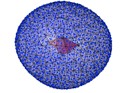
Figure 2: The equipotential surface given by Eq. (6) with $U_{0}=-0.1$ surrounding the bicapped tetrahedron local minimum of LJ₆. The surface is triangulated into $1000$ faces. Blue dots indicate the centers of the faces.

We surround every local minimum $i$ of LJ_N with the equipotential surface $\Sigma$ given by Eq. (6), and triangulate it:

$$\Sigma=\bigcup_{m=1}^{M}\sigma_{m},~{}~{}{\rm where}~{}\sigma_{m}\text{'s are triangular faces}.$$

The target value of $M$ is 1000. For each face center, we run minimization using the trust region BFGS method with a small maximal trust region radius and identify the minimum $j$ of LJ_N+1 to which the run converges. For $N\leq 8$, it suffices to compare the energy value of the found minimum with the energies of the minima of LJ_N+1. For larger $N$, if the energy of the found minimum coincides with that of a minimum $j$ of LJ_N+1 up to the prescribed tolerance, we look for an orthogonal transformation that aligns the found minimum with the minimum $j$. The transition probability $\gamma^{N\rightarrow N+1}_{ij}$ from minimum $i$ of LJ_N to minimum $j$ of LJ_N+1 is estimated using the formula:

$$\gamma^{N\rightarrow N+1}_{ij}=\frac{\sum_{m=1}^{M}A(\sigma_{m})\delta_{ij}(m)}{A(\Sigma)},$$ (7)

where $A(\sigma_{m})$ is the area of the triangular element $\sigma_{m}$, $A(\Sigma)$ is the area of the surface $\Sigma$, and $\delta_{ij}(m)=1$ if and only if the minimization run for minimum $i$ and face $m$ converges to minimum $j$, and $\delta_{ij}(m)=0$ otherwise.

Thus, we connect every pair of vertices $i$ in LJ_N and $j$ in LJ_N+1 with the arc $(i\rightarrow j)$ whenever $\gamma^{N\rightarrow N+1}_{ij}>0$. Given the attachment rate $\mu$, the transition rate along the arc $(i\rightarrow j)$ is $\mu\gamma^{N\rightarrow N+1}_{ij}$.

Such a connection of LJ_N and LJ_N+1 renders the resulting Markov chain time-irreversible and reducible. Each LJ_N component except for the last one created LJ₁₄ is transient, since the attachment causes the process to leave each LJ_N to LJ_N+1 without the possibility of return.

The created network LJ_6-14 is visualized in Fig. 3. Each LJ_N is presented as a black disconnectivity graph [3], while selected arcs from LJ_N to LJ_N+1 are depicted with catenary-shaped colored curves. An arc $(i\rightarrow j)$ from LJ_N to LJ_N+1 is shown if and only if $i$ is one of the 50 lowest minima of LJ_N and $\gamma^{N\rightarrow N+1}_{ij}>0.1$.

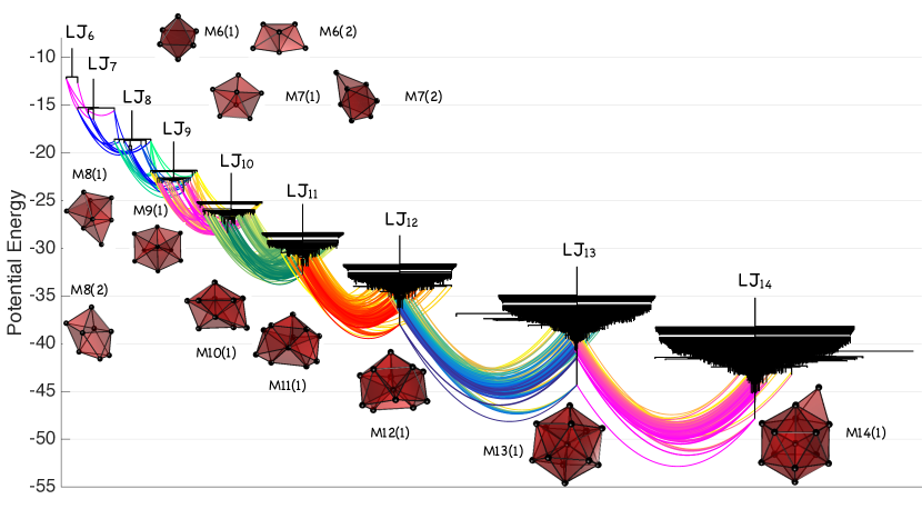
Figure 3: The LJ_6-14 aggregation/deformation network. The components LJ_N are visualised as disconnectivity graphs, while selected arcs from LJ_N to LJ_N+1 are depicted with catenary-shaped colored curves. An arc $(i\rightarrow j)$ from LJ_N to LJ_N+1 is shown if and only if $i$ is one of the 50 lowest minima of LJ_N and $\gamma^{N\rightarrow N+1}_{ij}>0.1$. For each LJ_N, the global minimum as well as some local minima are shown. M$N(n)$ denotes the $n$th lowest minimum of LJ_N.

The statistics for the LJ_6-14 network are presented in Table 1.

Table 1: The statistics of the aggregation/deformation LJ_6-14 network. $N$ is the number of atoms, “# min” is the number of minima, “# ts” is the number of found transition states (Morse-index one saddles), “# ts, $i\neq j$” is the number of transition states connecting minima mapped to distinct vertices of LJ_N, “$i\neq j$, $\exists$ ts_ij” is the number of unordered sets of two vertices of LJ_N connected by an edge, i.e., half the number of nonzero off-diagonal entries in the generator matrix $L_{N}$, “$\langle$degree$\rangle$” is the mean vertex degree of the LJ_N network, “max degree” is the maximal vertex degree of the LJ_N network (the vertex index (indices) where it is achieved is indicated in the parentheses), “#min0” is the number of vertices $j$ in LJ_N such that there is $i$ in LJ_N-1 such that $\gamma^{{N-1}\rightarrow N}_{ij}>0$.

$N$	# min	# ts	# ts, $i\neq j$	$i\neq j$, $\exists$ tsij	$\langle$degree$\rangle$	max degree	# min0
6	2	3	1	1	1	1 (1,2)	1
7	4	10	6	5	3	4 (1)	4
8	8	51	30	16	7.5	18 (1)	8
9	21	61	56	45	5.33	16 (5)	15
10	63	938	700	372	22.2	117 (5)	60
11	169	756	722	648	8.54	53 (12)	165
12	515	1582	1525	1410	6.04	152 (1)	487
13	1510	4660	4512	4290	5.98	306 (1)	1450
14	4135	13049	12630	11823	6.11	1822 (1)	4109

3 Analysis of the Aggregation/Deformation LJ_6-14 network

The LJ_6-14 aggregation/deformation network is time-irreversible and reducible. Its states lying in LJ_N for $6\leq N\leq 13$ are transient. In addition, although we did not compute the LJ₁₅ network, we can assume that a new atom attaches to LJ₁₄ as happens for LJ_N, $N\leq 13$, and treat the LJ₁₄ component as transient as well. This is equivalent to adding an additional vertex $v_{15}$ to LJ_6-14 representing LJ₁₅, shooting arcs from every vertex of LJ₁₄ to $v_{15}$, and setting the transition rates along these arcs to $\mu$. We would like to study the relaxation process in the LJ_6-14 network starting at M6(2), the bicapped tetrahedron local minimum of LJ₆, that is obtained from the only minimum of LJ₅ by attaching an extra atom. The proposed analysis approach is described in Section 3.1. Central to it is the calculation of the expected initial and pre-attachment distributions for each LJ_N, $6\leq N\leq 14$. The results are presented in Section 3.2. In Section 3.3, the obtained expected initial and pre-attachment distributions are compared to the invariant distribution for each LJ_N. Finally, a structural analysis of local energy minima is conducted in Section 3.4, and the formation mechanism of configurations with icosahedral packing is investigated.

3.1 Analysis method

For each number of atoms $N$, $6\leq N\leq 14$, we compute two probability distributions: the expected probability distribution LJ_N after the attachment of the $N$th atom, and the expected distribution in LJ_N right before the attachment of the $(N+1)$st atom. We refer to them as the expected initial and pre-attachment distributions and denote them by $p^{N}_{0}$ and $p^{N}_{e}$ respectively.

The expected initial distribution for LJ₆ is $p^{6}_{0}=[0,1]$, where $0$ corresponds to the global minimum M6(1), the octahedron, while $1$ corresponds the bicapped tetrahedron M6(2).

The expected pre-attachment distribution for LJ_N can be found as follows. We consider two random variables: the continuous random variable $T$, the attachment time, i.e., the time between the arrivals of two consecutive new atoms, and the discrete random variable $S$, which indicates the state/vertex immediately before attachment. The joint probability density $f^{N}_{S,T}(s,t)$ can be expressed as

$$f_{S,T}^{N}(s,t)=\mathbb{P}^{N}(S=s|T=t)f_{T}(t).$$ (8)

We assume that $T$ is an exponentially distributed random variable with the probability density function $f_{T}(t)=\mu e^{-\mu t}$.

The probability $\mathbb{P}^{N}(S=s|T=t)$ can be found from the following considerations. Suppose that the initial probability distribution in LJ_6-14 is supported within LJ_N, where $6\leq N\leq 14$. Let $p^{N}(t)$ be the subset of components of the probability distribution corresponding to the set of states of LJ_N. The conditional probability distribution $\hat{p}^{N}(t)$ in LJ_N conditioned on the fact that the system remains in LJ_N at time $t$ is given by

$$\hat{p}^{N}(t)=\sum_{k=0}^{M_{N}-1}(p^{N}_{0}\phi_{N}^{k})e^{-\lambda_{N}^{k}t}(P_{N}\phi_{N}^{k})^{T},\quad 0\leq t<T.$$ (9)

Here $M_{N}$ is the number of states in LJ_N; $p^{N}_{0}=p^{N}(0)$ is the initial distribution; $-\lambda^{k}_{N}$’s are the eigenvalues of $L_{N}$, the restriction of the generator matrix of LJ_6-14 to LJ_N; $\phi_{N}^{k}$ and $(P_{N}\phi_{N}^{k})^{T}$ are the corresponding right and left eigenvectors respectively; $P_{N}$ is the diagonal matrix with the invariant distribution $\pi_{N}$ for LJ_N given by Eq. (3) along its diagonal. The eigenvectors are normalized so that $\Phi_{N}\Phi_{N}^{T}P_{N}=\Phi_{N}^{T}P_{N}\Phi_{N}=I$, where $\Phi_{N}=[\phi^{0}_{N},\ldots,\phi_{N}^{M_{N}-1}]$ is the matrix whose columns are the right eigenvectors. Hence, right before the arrival of the new atom at time $t$, $\mathbb{P}(S=s|T=t)=\hat{p}_{s}^{N}(t)$, the $s$th component of $\hat{p}^{N}(t)$.

Integrating out the attachment time $T$, we obtain the expected probability distribution at the moment right before the arrival of the $(N+1)$st atom:

$$p^{N}_{e}(s)\equiv\mathbb{P}^{N}(S=s) =\int_{0}^{\infty}{f_{S,T}^{N}(s,t)dt}$$

$$=\int_{0}^{\infty}{\mathbb{P}^{N}(S=s|T=t)f_{T}(t)dt}$$

$$=\int_{0}^{\infty}{\hat{p}^{N}_{s}(t)\mu e^{-\mu t}dt}$$

$$=\mu\sum_{k=0}^{N-1}(p^{N}_{0}\phi_{N}^{k})\left(\int_{0}^{\infty}{e^{-(\mu+\lambda^{k}_{N})t}dt}\right)(P_{N}\phi_{N}^{k})^{T}_{s}$$

$$=\sum_{k=0}^{N-1}(p^{N}_{0}\phi_{N}^{k})\left(\frac{\mu}{\mu+\lambda_{N}^{k}}\right)(P_{N}\phi_{N}^{k})^{T}_{s}.$$ (10)

Therefore, the expected pre-attachment distribution is given by

$$p_{e}^{N}=\mu p_{0}^{N}\Phi_{N}(\mu I-\Lambda_{N})^{-1}\Phi_{N}^{T}P_{N}=\mu p_{0}^{N}(\mu I-L_{N})^{-1},$$ (11)

where $\Lambda_{N}={\rm diag}\{0,-\lambda_{N}^{1},\ldots,-\lambda_{N}^{M_{N}-1}\}$.

Once the expected pre-attachment distribution $p_{e}^{N}$ is computed using Eq. (11), one can obtain the expected initial distribution for LJ_N+1 by multiplying the pre-attachment distribution by the $M_{N}\times M_{N+1}$ transition matrix $\Gamma^{N\rightarrow N+1}=(\gamma^{N\rightarrow N+1}_{ij})$, where $\gamma^{N\rightarrow N+1}_{ij}$ are given by Eq. (7):

$$p_{0}^{N+1}=p_{e}^{N}\Gamma^{N\rightarrow N+1}.$$ (12)

Starting from $p_{0}^{6}=[0,1]$ and using Eqs. (11) and (12), one can compute the sequence of the expected pre-attachment and initial distributions $p_{e}^{N}$ and $p_{0}^{N+1}$ for $6\leq N\leq 13$ and the pre-attachment distribution $p_{e}^{14}$.

3.2 The sequence of the initial and the pre-attachment distributions

We have calculated the expected initial and pre-attachment distributions for the transient LJ_N networks, $6\leq N\leq 14$, for the range of attachment rates $10^{-4}\leq\mu\leq 10^{4}$ and three values of temperatures: $k_{B}T\equiv\beta^{-1}=0.06$, 0.08, and 0.10. As was mentioned in Section 1.2, the temperature should be low enough to justify the assumption that detachments can be neglected. A reasonable criterion for choosing appropriate temperature values is that they lie below the maximizer of the heat capacity[10] of the cluster LJ_N corresponding to the major structural (phase) transition. In LJ_N, $7\leq N\leq 14$, the single maximum of the heat capacity corresponds to the phase transition from solid to liquid-like configurations. We remind that the heat capacity of a cluster is given by

$$C_{v}(\beta^{-1}):=\frac{\partial\langle V\rangle}{\partial\beta^{-1}}=\frac{\partial}{\partial\beta^{-1}}\left(\frac{\sum_{i}V_{i}O_{i}^{-1}\sqrt{\det H_{i}}e^{-\beta V_{i}}}{\sum_{i}O_{i}^{-1}\sqrt{\det H_{i}}e^{-\beta V_{i}}}\right),$$

where the sum is taken over all minima $i$ of LJ_N. Fig. 4 shows that our chosen temperatures $\beta^{-1}=0.06$, 0.08, and 0.10 are below the maximizers of the heat capacity $C_{v}$ for clusters LJ_N, $7\leq N\leq 14$, and around it for LJ₆. Note that the only structural transition in LJ₆ is the one from the dominance of M6(1), the octahedron, to the dominance of M6(2). LJ₆ is too small to admit liquid-like states.

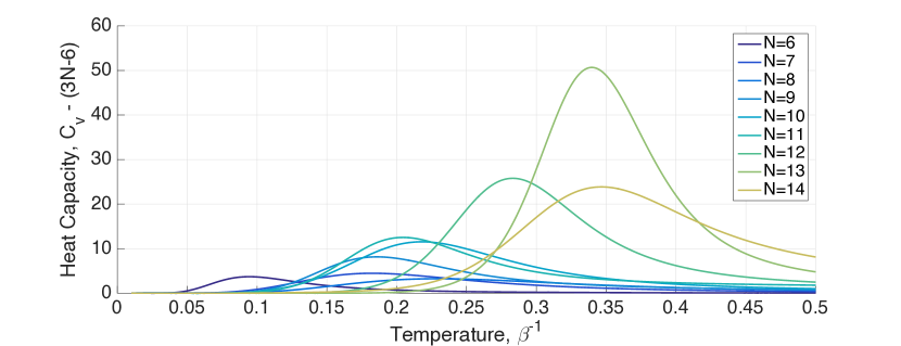
Figure 4: The heat capacities $C_{v}-(3N-6)$ for LJ_N networks, $6\leq N\leq 14$.

The resulting distributions for $10^{-4}\leq\mu\leq 10^{4}$ are shown in Figs. 5, 6, and 7 for $\beta^{-1}=0.06,~{}0.08$, and $0.10$ respectively. To avoid cluttering near the $\mu$-axis, only those components of the distributions that attain at least 7% likelihood for some values of $\mu$ are shown.

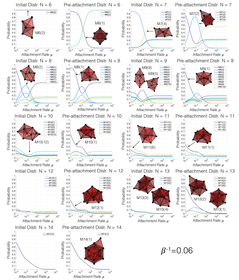
Figure 5: The expected initial and pre-attachment distributions for the aggregation process from $N=6$ to $N=14$ atoms at $\beta^{-1}=0.06$.

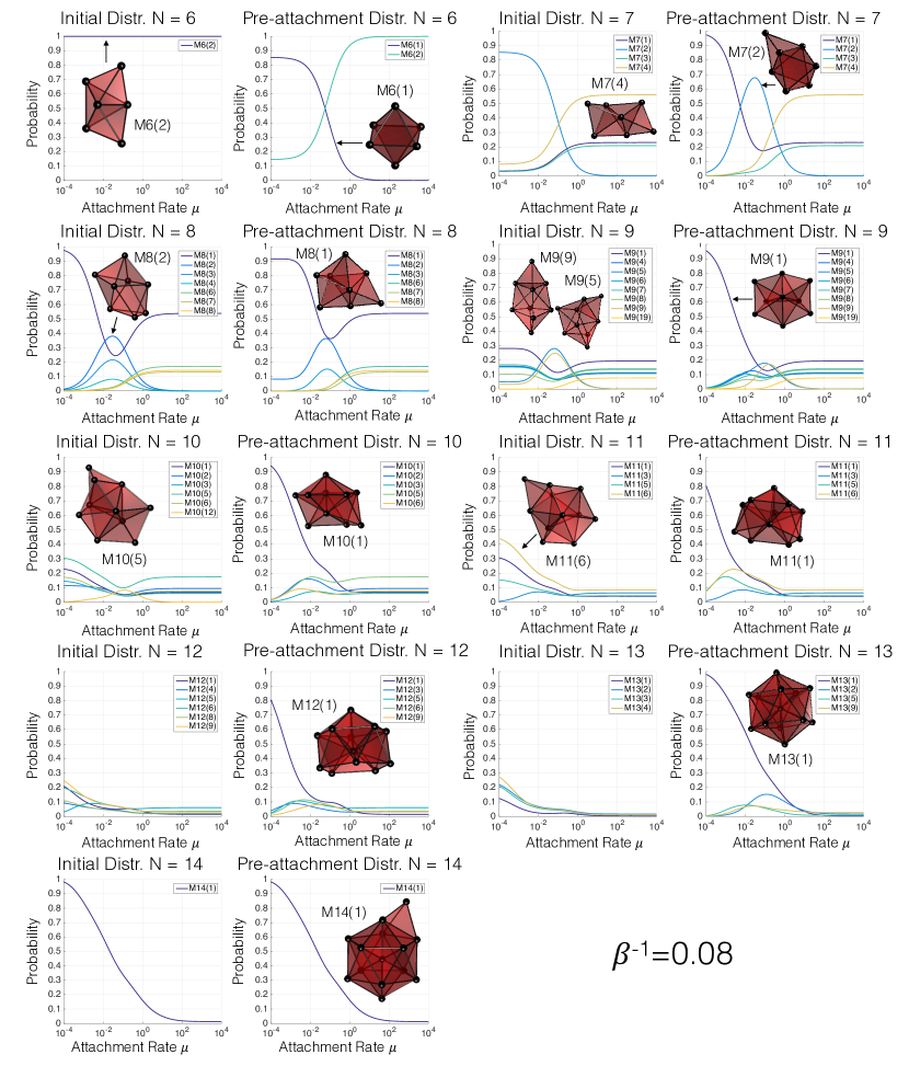
Figure 6: The expected initial and pre-attachment distributions for the aggregation process from $N=6$ to $N=14$ atoms at $\beta^{-1}=0.08$.

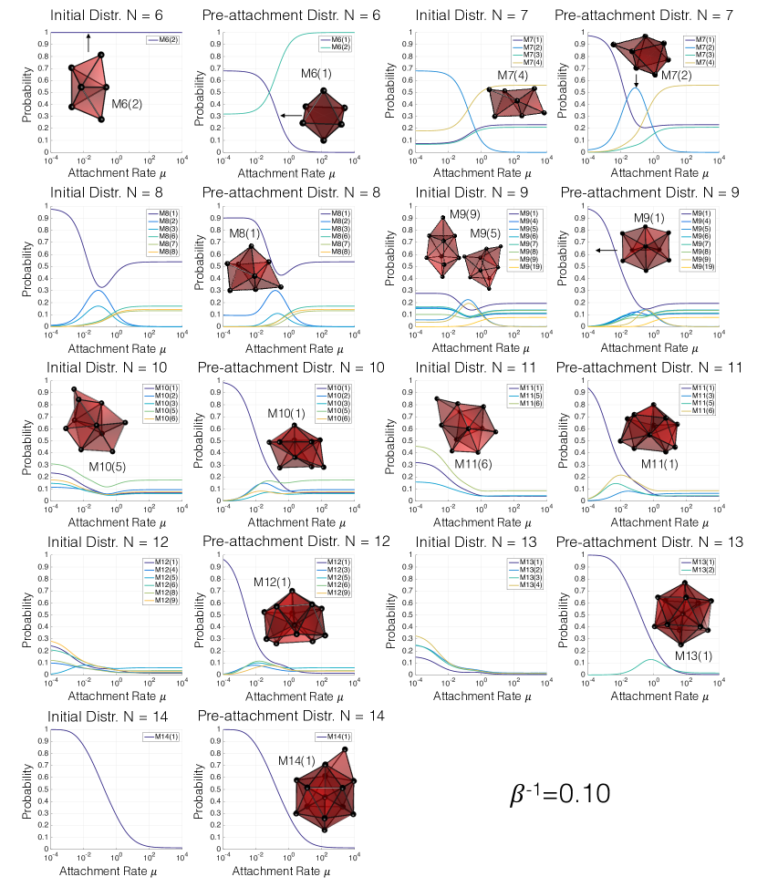
Figure 7: The expected initial and pre-attachment distributions for the aggregation process from $N=6$ to $N=14$ atoms at $\beta^{-1}=0.10$.

Eq. (10) implies that the expected pre-attachment distribution for LJ_N approaches the invariant distribution as $\mu\rightarrow 0$, and approaches the expected initial distribution as $\mu\rightarrow\infty$. Indeed, the factor ${\mu}(\mu+\lambda^{k}_{N})^{-1}$ tends to zero as $\mu\rightarrow 0$ for all $k\geq 1$, and tends to 1 as $\mu\rightarrow\infty$ for all $k\geq 0$. This is consistent with our results (Figs. 5 -7). For all $6\leq N\leq 14$, the expected pre-attachment distributions for $\mu=10^{-4}$ are nearly the invariant distributions at the corresponding values of $\beta$, while for $\mu=10^{4}$, they are nearly the corresponding expected initial distributions. As the attachment rate $\mu$ becomes large, the relaxation process in each LJ_N cluster is limited, resulting in broad expected initial and pre-attachment distributions as one can infer from Figs. 5-7.

The global minima for $7\leq N\leq 14$ are based on icosahedral packing (i.e., can be completed to nearly regular icosahedra merely by adding atoms), while the one for $N=6$ is the octahedron, which is an elementary cell of a face-centered cubic crystal. The transitions from the global minima of LJ_N to configurations of LJ_N+1, $6\leq N\leq 14$, happening with probabilities at least 0.1 are illustrated in Fig. 8.

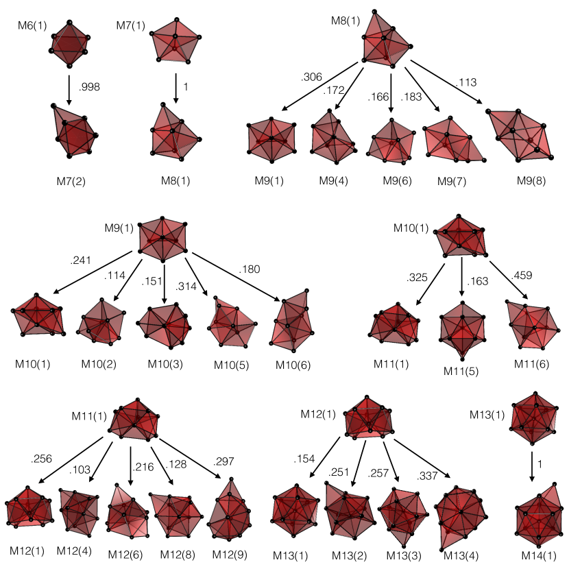
Figure 8: The transitions from the global minima of LJ_N to configurations of LJ_N+1, $6\leq N\leq{13}$, happening with probabilities at least 0.1. The numbers next to the arrows indicate the transition probabilities.

One can observe two types of persisting clusters in Figs. 5 - 7: icosahedral and non-icosahedral. The probabilities of the heirs of the 6-atom octahedron, M7(2), M8(2), M8(3), M9(5), M9(9), and M10(12), peak in the mid-range of the attachment rate $\mu$ and are especially prominent for $\beta^{-1}=0.06$ (Fig. 5). A more complete heritage cascade of non-icosahedral clusters up to $N=10$ is shown in Fig. 9.

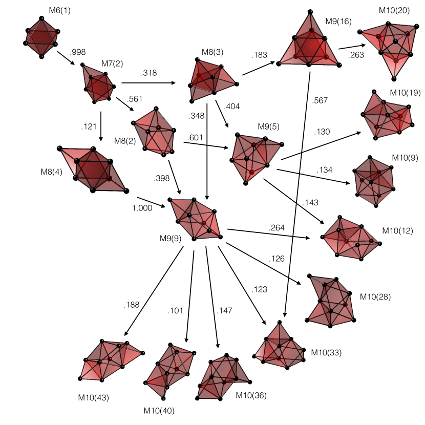
Figure 9: The heritage cascade of the global minimum M6(1) of LJ₆, the octahedron, for up to 10 atoms. All transition probabilities exceeding 0.1 are displayed. The numbers next to the arrows indicate the transition probabilities.

The icosahedral heritage cascade is partially displayed in Fig. 10 (partially, as it quickly becomes too broad). Comparing these cascades, we observe that the non-icosahedral one involves only high-energy minima of LJ₁₀: the lowest of them is M10(9). On the contrary, the icosahedral heritage cascade involves all global minima and many other low-energy minima for $7\leq N\leq 14$.

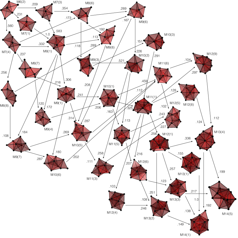
Figure 10: The heritage cascade of the minimum M6(2) of LJ₆, the bicapped trigonal bipyramid. Only some configurations with probabilities exceeding 0.1 in the expected initial or pre-attachment distributions in Figs. 5-7 and displayed, and only transition probabilities exceeding 0.1 are shown. The numbers next to the arrows indicate the transition probabilities.

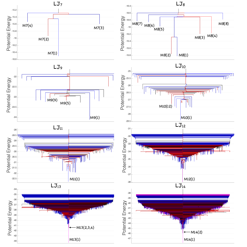
Figure 11: The disconnectivity graphs for $7\leq N\leq 14$. Blue ($b^{N}(i)>a^{N}(i)$) and magenta ($b^{N}(i)<a^{N}(i)$) leaves correspond to minima with icosahedral packing. Red ($b^{N}(i)<a^{N}(i)$) and black ($b^{N}(i)>a^{N}(i)$) leaves correspond to minima with non-icosahedral packing.

The aggregation process involves two kinds of processes: attachment and relaxation. In order to examine the aggregation process as $\mu\rightarrow\infty$, it is instructive to compare two aggregation processes involving only attachment, one starting from M6(1) and the other one starting from M6(2). The corresponding probability distributions for LJ_N are given, respectively, by

$$a^{N}:=[1,0]\Gamma^{6\rightarrow 7}\ldots\Gamma^{N-1\rightarrow N}\quad{\rm and}\quad b^{N}:=[0,1]\Gamma^{6\rightarrow 7}\ldots\Gamma^{N-1\rightarrow N}.$$ (13)

Now, for each state in each LJ_N network, $6\leq N\leq 14$, we compare the distributions $a^{N}$ and $b^{N}$. Fig. 11 displays the disconnectivity graphs where the states $i$ are plotted red/magenta or blue/black depending on whether $a^{N}(i)>b^{N}(i)$ or $a^{N}(i)<b^{N}(i)$ respectively. It is evident from Fig. 11 that the probabilities for the global minima of LJ_N, $12\leq N\leq 14$, to form starting from M6(1) are larger than those starting from M6(2). This is an interesting fact, and we investigate it in more detail.

Let $A_{N}$ and $B_{N}$ be the subsets of states of LJ_N defined by

$$A_{N}:=\{i~{}|~{}a^{N}(i)>b^{N}(i)\},\quad B_{N}:=\{i~{}|~{}a^{N}(i)<b^{N}(i)\}.$$ (14)

The numbers of states in $A_{N}$ and $B_{N}$ as well as the probabilities to find the LJ_N cluster in $A_{N}$ and $B_{N}$ assuming the invariant distribution in LJ_N for the temperatures $\beta^{-1}=0.06,0.08,0.10$ are shown in Table 2. The sizes of the sets $B_{N}$ grow slower than those of $A_{N}$, and $|A_{N}|$ surpasses $|B_{N}|$ at $N=10$. Meanwhile, the sets $A_{N}$ contain only low occupancy states for $N=7,8$, and extremely low occupancy (high energy) states for $N=9,10,11$. However, for $N\geq 12$, the sets $A_{N}$ acquire the global minima and their probabilities switch to almost one at the considered temperatures.

Table 2: The numbers of states in the sets $A_{N}$ and $B_{N}$, $7\leq N\leq 14$ defined by Eq. (14) and the probabilities to find the N-atom cluster in them assuming the invariant distributions in LJ_N.

$N$, $\beta^{-1}$	$|A_{N}|$, $\mathbb{P}(A_{N})$	$|B_{N}|$, $\mathbb{P}(B_{N})$
$\mathbf{N=7}$	$|A_{7}|=1$	$|B_{7}|=3$
0.06	3.797e-4	9.996e-1
0.08	4.072e-3	9.959e-1
0.10	1.667e-2	9.833e-1
$\mathbf{N=8}$	$|A_{8}|=3$	$|B_{8}|=5$
0.06	6.721e-2	9.328e-1
0.08	8.372e-3	9.163e-1
0.10	9.610e-2	9.039e-1
$\mathbf{N=9}$	$|A_{9}|=10$	$|B_{9}|=11$
0.06	2.445e-6	1
0.08	1.679e-4	1
0.10	2.359e-3	9.976e-1
$\mathbf{N=10}$	$|A_{10}|=38$	$|B_{10}|=25$
0.06	1.522e-7	1
0.08	1.789e-5	1
0.10	3.408e-4	9.996e-1
$\mathbf{N=11}$	$|A_{11}|=100$	$|B_{11}|=69$
0.06	1.023e-7	1
0.08	1.458e-5	1
0.10	3.666e-4	9.996e-1
$\mathbf{N=12}$	$|A_{12}|=331$	$|B_{12}|=170$
0.06	1	3.766e-11
0.08	1	4.781e-8
0.10	1	3.568e-6
$\mathbf{N=13}$	$|A_{13}|=1038$	$|B_{13}|=472$
0.06	1	1.802e-23
0.08	1	6.949e-17
0.10	1	6.398e-13
$\mathbf{N=14}$	$|A_{14}|=2877$	$|B_{14}|=1257$
0.06	1	4.787e-18
0.08	1	3.870e-13
0.10	1	3.514e-10

3.3 Comparison to Invariant Distributions

In this Section, we introduce the normalized root-mean-square (NRMS) deviation and use it to compare the computed expected initial and pre-attachment distributions to the invariant distribution for each LJ_N.

Let $\pi$ be a probability distribution. The most different from $\pi$ is the distribution $\chi(i_{\min})$ which assumes 1 at a state $i_{\min}:=\arg\min_{i}\pi_{i}$ and zeros at all other states. The normalized RMS deviation of a distribution $p$ in LJ_N from $\pi$ is defined as

$$d_{NRMS}(p,\pi):=\frac{\sqrt{\sum_{i}(p_{i}-\pi_{i})^{2}}}{\sqrt{\sum_{i}(\chi(i_{\min})_{i}-\pi_{i})^{2}}}$$ (15)

The NRMS deviations of the expected initial and pre-attachment distributions from the invariant distributions $\pi^{N}$ (Eq. (3)), $6\leq N\leq 14$, for $\beta^{-1}=0.06$, 0.08, and 0.10 are shown in Fig. 12 (a),(b),(c) respectively. For all $N$, as one would expect, $d_{NRMS}(p_{0}^{N},\pi^{N})$ and $d_{NRMS}(p_{e}^{N},\pi^{N})$ approach $d_{NRMS}(b^{N},\pi^{N})$ (the normalized RMS deviation of the asymptotic distribution $b^{N}$ (Eq. (13)) from $\pi^{N}$) as $\mu\rightarrow\infty$. As $\mu\rightarrow 0$, $d_{NRMS}(p_{0}^{N},\pi^{N})$ and $d_{NRMS}(p_{e}^{N},\pi^{N})$ approach $d_{NRMS}(\pi^{N-1}\Gamma^{N-1\rightarrow N},\pi^{N})$ and zero respectively. An interesting fact observed in Fig. 12 is that the deviations $d_{NRMS}^{N}(p_{0}^{N})$ for $N=7$ and $9\leq N\leq 13$ are far from 0 for all attachment rates $\mu$. In particular, $d_{NRMS}(p_{0}^{13},\pi^{13})$ is nearly constant. This means that the attachment of a new atom throws invariant distributions for $N=6$ and $8\leq N\leq 12$ far away from the invariant distributions in $N=7$ and $9\leq N\leq 13$ respectively, roughly as far as the distributions $b^{N}$. On the other hand, the global minima for $N=8$ and $N=14$ are formed with probability one from the global minima of LJ₇ and LJ₁₃ respectively (Fig. 8). This explains why the corresponding expected initial distributions are close to the invariant ones for low attachment rates $\mu$. This effect is notably stronger for LJ₁₄ because the global minimum of LJ₁₄ is much deeper than all other minima in LJ₁₄, while the two deepest minima of LJ₈ have close values of energy.

(a)
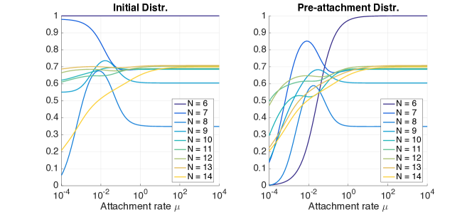
(b)
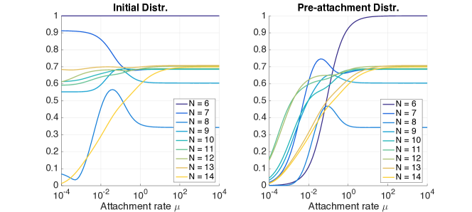
(c)

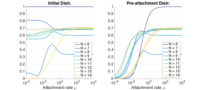
Figure 12: The normalized RMS deviations of the expected initial and pre-attachment distributions from the invariant distributions for $6\leq N\leq 14$. (a): $\beta^{-1}=0.06$. (b): $\beta^{-1}=0.08$. (c): $\beta^{-1}=0.10$.

3.4 Structural analysis

Fig. 11 and Table 2 suggest that the 6-atom octahedron M6(1) has a large icosahedral heritage that includes the global minima of LJ_N, $12\leq N\leq 14$. In this Section, we make the concepts of icosahedral or non-icosahedral packing more precise and quantify the structural transitions from icosahedral to non-icosahedral packings and vice versa during the attachment process.

We will call a local minimum M$N(i)$ of LJ_N icosahedral if the following two conditions hold:

1. every atom in M$N(i)$ is a vertex of a tetrahedron, whose vertices are a subset of 4 atoms of LJ_N, and edges are of length $2^{1/6}(1+\delta)$, where $|\delta|\leq\delta_{1}$;

2. no two atoms in M$N(i)$ are at distances $2^{1/6}\sqrt{2}(1+\delta)$, where $|\delta|\leq\delta_{2}$, or $2^{1/6}d(1+\delta)$, where $|\delta|\leq\delta_{3}$. The number $d$ is the distance between the pairs of atoms in M8(2) with 5 nearest neighbors, symmetric with respect to its symmetry plane (Fig. 13 (a)), $d\approx 1.269$.

Otherwise, we call a local minimum M$N(i)$ of LJ_N non-icosahedral. We emphasize that our definition of icosahedral and non-icosahedral minima refers to their packing rather than symmetry groups. Such a liberty is justified in the context of the study of aggregation, as any icosahedral minimum in the sense of our definition can be completed to a nearly regular icosahedron by the attachment of the right number of new atoms to the right places.

This definition is easy to check by a simple computer program. We set $\delta_{1}=\delta_{3}=0.1$ and $\delta_{2}=0.05$. The second condition renders minima such as M9(16), a tricapped octahedron (Fig. 9), non-icosahedral. In M9(16), every atom is a vertex of a tetrahedron; however, there is an octahedron in the middle.

Roughly speaking, the majority of local minima in Lennard-Jones clusters can be thought of being assembled out of building blocks shown in Fig. 13 (a): tetrahedron (cap), octahedron, M8(2), and hollow icosahedral shell. These blocks can be distorted to avoid cavities/overlaps. For example, M9(5) and M9(9) are capped M8(2), M10(28) is a bicapped M8(2) (Fig. 9), M13(1159) is a capped icosahedral shell. The numbers of icosahedral and some types of non-icosahedral minima are listed in Table 3. We did not split the types “M6(1) (octahedron) and M8(2)” as their “signature” interatomic distances, $d\approx 1.269$ and $\sqrt{2}\approx 1.414$, are close in comparison with our tolerances $\delta_{i}$, $i=1,2,3$. The only two non-icosahedral minima that are not of any of these listed types are those of LJ₁₄ shown in Fig. 13 (b): M14(43) consists of two hexagonal pyramids rotated by 30 degrees with respect to each other; M14(3422) has an atom that is not a part of any tetrahedron. While for $10\leq N\leq 14$ the numbers of icosahedral minima are less than those of non-icosahedral, one can check that the probabilities to find a cluster in an icosahedral minimum assuming the invariant distribution in LJ_N, $7\leq N\leq 14$, are very close to one.

(a)
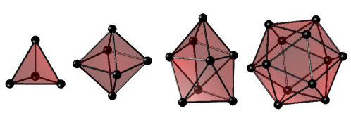
(b)

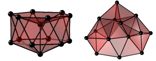
Figure 13: (a): The main building blocks of LJ clusters (left to right): the regular tetrahedron, the octahedron, the M8(2) configuration with the point group $D_{2h}$ of order 8, and the icosahedral shell. (b): The two found minima of LJ₁₄ that do not consist of the building blocks above: (left to right) M14(43) can be split to two hexagonal pyramids rotated with respect to each other, M14(3422) contains an atom (the one at the bottom) that is not a part of any tetrahedron.

Table 3: Structure of $N$-atom clusters. The column “ico” contains the numbers of icosahedral local minima. The column “M6(1) or M8(2)” contains the numbers of local minima involving some interatomic distances characteristic of the octahedron or the M8(2). The column “ico shell” contains the numbers of local minima involving the 12-atom icosahedral shell, capped for LJ₁₃ and bicapped for LJ₁₄. The column “other” contains the numbers of non-icosahedral local minima of none of the above types.

$N$	ico	M6(1) or M8(2)	ico shell	other
6	1	1	0	0
7	3	1	0	0
8	5	3	0	0
9	11	10	0	0
10	26	37	0	0
11	72	97	0	0
12	175	339	1	0
13	483	1026	1	0
14	1286	2842	5	2

Transition probabilities from icosahedral/non-icosahedral minima of LJ_N to icosahedral/non-icosahedral minima of LJ_N+1 as a result of attachment of a new atom are displayed in Table 4. Evidently, icosahedral minima tend to transition to icosahedral ones, and non-icosahedral minima tend to transition to non-icosahedral ones. However, the transition probabilities from icosahedral to non-icosahedral minima and non-icosahedral to icosahedral ones are nonzero; the latter probabilities exceed the former by about an order of magnitude, and are significant for $11\leq N\leq 13$.

Table 4: Transition probabilities from icosahedral/non-icosahedral local minima of LJ_N to icosahedral/non-icosahedral local minima of LJ_N+1. “ico” and “nico” abbreviate “icosahedral” and “non-icosahedral ” respectively.

$N\rightarrow N+1$	$\mathbb{P}($ico $\rightarrow$ ico$)$	$\mathbb{P}($ico $\rightarrow$ nico$)$	$\mathbb{P}($nico $\rightarrow$ ico$)$	$\mathbb{P}($nico $\rightarrow$ nico$)$
$6\rightarrow 7$	1	0	1.634e-4	9.998e-1
$7\rightarrow 8$	9.993e-1	6.702e-4	2.315e-4	9.998e-1
$8\rightarrow 9$	1	0	2.540e-4	9.997e-1
$9\rightarrow 10$	9.997e-1	2.960e-4	1.118e-3	9.989e-1
$10\rightarrow 11$	9.993e-1	7.112e-4	5.002e-3	9.950e-1
$11\rightarrow 12$	9.935e-1	6.534e-3	7.440e-2	9.926e-1
$12\rightarrow 13$	9.926e-1	7.436e-3	1.570e-1	8.430e-1
$13\rightarrow 14$	9.893e-1	1.071e-2	2.272e-1	7.728e-1

Tables 5 and 6 list the numbers of icosahedral and non-icosahedral minima in the distributions $a^{N}$ and $b^{N}$, $6\leq N\leq 14$, together with their probabilities. The distributions $a^{N}$ contain both icosahedral and non-icosahedral clusters in comparable proportions for $12\leq N\leq 14$. In contrast to this fact, the distributions $b^{N}$ contain primarily icosahedral minima.

Therefore, the two kinds of processes, relaxation and attachment, involved in the aggregation process up to 14 atoms lead to the formation of icosahedral clusters for $N\geq 11$. Relaxation does so because the global minima of LJ_N, $7\leq N\leq 14$, are icosahedral. Attachment favors icosahedral minima because icosahedral minima transition primarily to icosahedral ones, while non-icosahedral minima start to transition to both icosahedral and non-icosahedral ones with comparable probabilities for $11\leq N\leq 13$.

Table 5: The structure of local minima in the distributions $a^{N}$ (Eq. (13)). The columns “ico” and “nico” contain the numbers of icosahedral/non-icosahedral local minima respectively corresponding to nonzero entries in the distributions $b^{N}$, and the columns “$\mathbb{P}$(ico)” and “$\mathbb{P}$(nico)” contain their probabilities.

$N$	ico	$\mathbb{P}$(ico)	nico	$\mathbb{P}$(nico)
7	1	1.634e-4	1	9.998e-1
8	2	3.949e-4	3	9.996e-1
9	9	8.221e-4	4	9.992e-1
10	23	8.390e-4	22	9.992e-1
11	68	4.336e-3	64	9.957e-1
12	171	1.151e-1	233	8.492e-1
13	475	3.251e-1	709	6.749e-1
14	1264	4.828e-1	1987	5.172e-1

Table 6: The structure of local minima in the distributions $b^{N}$ (Eq. (13)). The columns “ico” and “nico” contain the numbers of icosahedral/non-icosahedral local minima respectively corresponding to nonzero entries in the distributions $b^{N}$, and the columns “$\mathbb{P}$(ico)” and “$\mathbb{P}$(nico)” contain their probabilities.

$N$	ico	$\mathbb{P}$(ico)	nico	$\mathbb{P}$(nico)
7	3	1	0	0
8	5	9.991e-1	1	8.962e-4
9	11	9.991e-1	2	8.955e-4
10	25	9.990e-1	16	9.969e-4
11	69	9.988e-1	58	1.165e-3
12	171	9.982e-1	220	1.831e-3
13	475	9.978e-1	687	2.203e-3
14	1264	9.967e-1	1955	3.263e-3

4 Perspectives

The aggregation/deformation LJ_6-14 network constructed and analyzed in this work is a model for an isothermal aggregation process, i.e., some amount of energy is taken away from to the cluster as it acquires a new atom in such a manner that the mean kinetic energy per atom remains constant. In this work, we had only one control parameter, the attachment rate $\mu$. We assumed that the attachment time was an exponentially distributed random variable with a fixed parameter $\mu$ for all $N$. We did not allow detachments of atoms. Our analysis of this simple aggregation model showed that both processes taking place in the system, attachment and relaxation, promote icosahedral packing.

Our results encourage us to examine more sophisticated aggregation models, in particular, enabling detachments, in our future work. Figs. 5 – 7 suggest the conjecture that the primary mechanism of the formation of the 13-atom icosahedron is from the global minimum of LJ₁₄, the capped icosahedron: the “cap” atom detaches from the icosahedron. Each atom on the surface of the 13-atom icosahedron has 6 nearest neighbors, which makes it extremely stable. This would explain the notable peaks in the mass spectra in [15, 20] at $N=13$. Presumably, a similar mechanism takes place for other clusters with magic numbers of atoms.

Besides allowing detachments, the study of aggregation processes by means of stochastic networks can be continued in several other directions. First, one can continue building LJ_6-N aggregation/deformation networks for $N>14$. Due to the exponential growth of the number of local minima in LJ_N with $N$ (Eq. (4)), it will be necessary to use some kind of importance sampling on the set of local minima, e.g., the basin hopping method [37, 38]. For example, Wales’s datasets for LJ₃₈ [43] and LJ₇₅ contain $100\thinspace 000$ and $593\thinspace 320$ local minima respectively, while the predicted numbers of local minima in them according to Eq. (4) are of the orders of $10^{14}$ and $10^{31}$ respectively.

Second, one can consider a non-isothermal aggregation and make the attachment rate $\mu$ dependent on the current number of atoms in the cluster. For example, one can imagine a fixed number of interacting macroscopic particles (e.g., ball-shaped macromolecules) that are allowed to self-assemble in a small closed container filled with solvent (e.g., see experiments conducted with microgel balls in [30]).

Finally, our methodology of the study of aggregation process of Lennard-Jones particles by means of stochastic networks is transferable to the study of self-assembly of particles interacting according to other kinds of potentials. The dream of design by self-assembly inspired research on the self-assembly of micron-size particles interacting according to a short-range potential [1, 30, 23, 24], limited to a fixed number of particles so far. Allowing new particles to arrive at a controlled rate and regulating the temperature will upgrade the ability to obtain desired configurations of particles.

The present work can be considered as the first step toward the goal of generating desired types of clusters by means of controlled aggregation/self-assembly.

References

- [1] N. Arkus, V. Manoharan and M. P. Brenner, Minimal Energy Clusters of Hard Spheres with Short Ranged Attractions, Phys Rev Lett, 103,118303 (2009).
- [2] F. Baletto, A. Rapallo, G. Rossi, and R. Ferrando, Dynamical effects in the formation of magic cluster structures, Phys. Rev. B 69, 235421 (2004)
- [3] O. M. Becker, and M. Karplus, The topology of multidimensional potential energy surfaces: Theory and application to peptide structure and kinetics, J. Chem. Phys. 106 (4), 1495 (1997)
- [4] F. Calvo, D. Schebarchov, and D. J. Wales, Grand and Semigrand Canonical Basin-Hopping, J. Chem. Theory Comput. 12, 902 - 909 (2016)
-
[5]
https://www.math.umd.edu/~mariakc/lennard-jones.html
- [6] M. Cameron and E. Vanden-Eijnden, Flows in Complex Networks: Theory, Algorithms, and Application to Lennard-Jones Cluster Rearrangement, J. Stat. Phys., 156, 3, 427-454 (2014)
- [7] M. K. Cameron, Metastability, Spectrum, and Eigencurrents of the Lennard-Jones-38 Network, J. Chem. Phys., 141, 184113 (2014)
- [8] M. K. Cameron and T. Gan, Spectral analysis and clustering of large stochastic networks. Application to the Lennard-Jones-75 cluster. Molecular Simulation, 42, 16, 1410-1428 (2016)
- [9] J. M. Carr and D. J. Wales, Folding Pathways and Rates for the Three-Stranded -Sheet Peptide Beta3s using Discrete Path Sampling, J. Phys. Chem. B, 112, 8760-8769 (2008)
- [10] J. P. K. Doye, D. J. Wales, and M. A. Miller, Thermodynamics and the global optimization of Lennard-Jones clusters, J. Chem. Phys. 109, 8143 (1998)
- [11] J. P. K. Doye, D. J. Wales, and M. A. Miller, The double-funnel energy landscape of the 38-atom Lennard-Jones cluster, J. Chem. Phys. 110, 6896 (1999)
- [12] W. E, W. Ren, and E. Vanden-Eijnden, String method for the study of rare events, Phys. Rev. B: 66, 052301 (2002)
- [13] W. E, W. Ren, and E. Vanden-Eijnden, Simplified and improved string method for computing the minimum energy paths in barrier-crossing events, J. Chem. Phys.: 126,164103 (2007)
- [14] W. E and X. Zhou, The gentlest ascend dynamics, Nonlinearity, 24, 1831-1842 (2011)
- [15] O. Echt, K. Sattler, and E. Recknagel, Magic Numbers for Sphere Packings: Experimental Verification in Free Xenon Clusters, Phys. Rev. Lett., 47, 16, 1121-1124 (1981)
- [16] O. Echt and O. Kandler and T. Leisner and W. Mlechle and E. Recknagel, Magic Numbers in Mass Spectra of Large van der Waals Clusters J. Chem. Soc. Faraday Trans., 86, 2411 (1990)
- [17] J. Farges and M. F. de Feraudy and B. Raoult and G. Torchet, Structure and temperature of rare gas clusters in a supersonic expansion, Surface Science 106, 95, (1981)
- [18] S. N. Fejer and D. J. Wales, Helix Self-Assembly from Anisotropic Molecules, Phys. Rev. Letters, 99, 086106 (2007)
- [19] W. Gao, J. Leng, and X. Zhou, Iterative minimization algorithm for efficient calculations of transition states, J. Comp. Phys., 309, 69 87 (2016)
- [20] I. A. Harris and R. S. Kidwell and J. A. Northby, Structure of charged argon clusters formed in free jet expansion, Phys. Rev. Lett., 53, 2390 (1984)
- [21] I. A. Harris and K. A. Norman and R. V. Mulkern and J. A. Northby, Icosahedral structure of large charged argon clusters, Chem. Phys. Lett., 130, 316 (1986)
- [22] G. Henkelman and H. Jonsson, A dimer method for finding saddle points on high dimensional potential surfaces using only first derivatives, J. Chem. Phys., 111, 7010 (1999).
- [23] M. Holmes-Cerfon, S. J. Gortler, M. P. Brenner, A geometrical approach to computing free-energy landscapes from short-ranged potentials, Proc. Natl. Acad. Sci. 110 , 1, E5 - E14 (2013)
- [24] M. Holmes-Cerfon, Sticky-sphere clusters, Annual Reviews of Condensed Matter Physics, In press (expected 8, March 10, 2017).
- [25] H. Jonsson, G. Mills, K. W. Jacobsen, Nudged Elastic Band Method for Finding Minimum Energy Paths of Transitions, in Classical and Quantum Dynamics in Condensed Phase Simulations, Ed. B. J. Berne, G. Ciccotti and D. F. Coker, 385 (World Scientific, 1998).
- [26] S. Kakar, O. Bjoerneholm, J. Weigelt, A. R. B. de Castro, L. Troeger, R. Frahm, and T. Moeller, Size-dependent K-edge EXAFS study of the structure of free Ar clusters, Phys. Rev. Lett. 78, 9, 1675-1678 (1997)
- [27] S. I. Kovalenko and D. D. Solnyshkin and E. T. Verkhovtseva and V. V. Eremenko, Experimental detection of stacking faults in rare gas clusters Chem. Phys. Lett., 250, 309 (1996)
- [28] J. S. Langer, Statistical Theory of the Decay of Metastable States, Ann. Phys. 54, 258-275 (1969)
- [29] V. A. Mandelshtam and P. A. Frantsuzov, Multiple structural transformations in Lennard-Jones clusters: Generic versus size-specific behavior, J. Chem. Phys. 124, 204511 (2006)
- [30] G. Meng, N. Arkus, M.P. Brenner and V. Manoharan, The Free Energy Landscape of Hard Sphere Clusters, Science 327, 560 (2010)
- [31] M. A. Miller and D. J. Wales, Isomerization dynamics and ergodicity in Ar 7, J. Chem. Phys. 107, 8568 (1997)
- [32] L. J. Munro and D. J. Wales, Defect migration in crystalline silicon, Phys. Rev. B, 59, 3969-3980 (1999)
- [33] J. Nocedal and S. J. Wright, Numerical Optimization, Second Edition, Springer, USA, 2006
- [34] M. Picciani, M. Athenes, J. Kurchan, and J. Taileur, Simulating structural transitions by direct transition current sampling: the example of LJ38, J. Chem. Phys. 135, 034108 (2011)
- [35] F. H. Stillinger, Exponential multiplicity of inherent structures, Phys. Rev. E, 59, 1, 48-51 (1999)
- [36] D. C. Wallace, Statistical mechanics of monatomic liquids, Phys. Rev. E, 56, 4, 4179-4186 (1997)
- [37] D. J. Wales and J. P. K. Doye, Global Optimization by Basin-Hopping and the Lowest Energy Structures of Lennard-Jones Clusters Containing up to 110 Atoms, J. Phys. Chem. A, 101, 5111-5116, (1997)
- [38] D. J. Wales, Discrete Path Sampling, Mol. Phys., 100 (2002), 3285-3306
- [39] B. W. van de Waal, No Evidence for Size-Dependent Icosahedral fcc Structural Transition in Rare-Gas Clusters, Phys. Rev. Lett., 76, 7, 1083-1086 (1996)
- [40] D. J. Wales, “Energy Landscapes: Applications to Clusters, Biomolecules and Glasses”, Cambridge University Press, 2003
- [41] D. J. Wales, Energy landscapes: calculating pathways and rates, International Review in Chemical Physics, 25, 1-2, 237-282 (2006)
- [42] D. J. Wales, Energy Landscapes of Clusters Bound by Short-Ranged Potentials, J. Chem. Phys. and Phys. Chem., 11, 12, 2491-2494 (2010)
-
[43]
http://www-wales.ch.cam.ac.uk/CCD.html
- [44] J. Zhang and Q. Du, Shrinking dimer dynamics and its applications to saddle point search, SIAM J. Numer. Anal., 50, 4, 1899-1921 (2012)