Multiband variability studies and novel broadband SED modeling of Mrk 501 in 2009

Abstract

Aims. We present an extensive study of the BL Lac object Mrk 501 based on a data set collected during the multi-instrument campaign spanning from 2009 March 15 to 2009 August 1, which includes, among other instruments, MAGIC, VERITAS, Whipple 10 m, and Fermi-LAT to cover the $\gamma$-ray range from 0.1 GeV to 20 TeV, RXTE and Swift to cover wavelengths from UV to hard X-rays, and GASP-WEBT that provides coverage of radio and optical wavelengths. Optical polarization measurements were provided for a fraction of the campaign by the Steward and St.Petersburg observatories. We evaluate the variability of the source and interband correlations, the $\gamma$-ray flaring activity occurring in May 2009, and interpret the results within two synchrotron self-Compton (SSC) scenarios.

Methods. The multiband variability observed during the full campaign is addressed in terms of the fractional variability, and the possible correlations are studied by calculating the discrete correlation function for each pair of energy bands, where the significance was evaluated with dedicated Monte Carlo simulations. The space of SSC model parameters is probed following a dedicated grid-scan strategy, allowing for a wide range of models to be tested and offering a study of the degeneracy of model-to-data agreement in the individual model parameters, hence providing a less biased interpretation than the “single-curve SSC model adjustment” typically reported in the literature.

Results. We find an increase in the fractional variability with energy, while no significant interband correlations of flux changes are found on the basis of the acquired data set. The SSC model grid-scan shows that the flaring activity around May 22 cannot be modeled adequately with a one-zone SSC scenario (using an electron energy distribution with two breaks), while it can be suitably described within a two-independent-zone SSC scenario. Here, one zone is responsible for the quiescent emission from the averaged 4.5-month observing period, while the other one, which is spatially separated from the first, dominates the flaring emission occurring at X-rays and very high energy ($>$ 100 GeV, VHE) $\gamma$-rays. The flaring activity from May 1, which coincides with a rotation of the electric vector polarization angle (EVPA), cannot be satisfactorily reproduced by either a one-zone or a two-independent-zone SSC model, yet this is partially affected by the lack of strictly simultaneous observations and the presence of large flux changes on sub-hour timescales (detected at VHE $\gamma$-rays).

Conclusions. The higher variability in the VHE emission and lack of correlation with the X-ray emission indicate that, at least during the 4.5-month long observing campaign in 2009, the highest-energy (and most variable) electrons that are responsible for the VHE $\gamma$-rays do not make a dominant contribution to the $\sim$1 keV emission. Alternatively, there could be a very variable component contributing to the VHE $\gamma$-ray emission in addition to that coming from the SSC scenario. The studies with our dedicated SSC grid-scan show that there is some degeneracy in both the one-zone and the two-zone SSC scenarios probed, with several combinations of model parameters yielding a similar model-to-data agreement, and some parameters better constrained than others. The observed $\gamma$-ray flaring activity, with the EVPA rotation coincident with the first $\gamma$-ray flare, resembles those reported previously for low frequency peaked blazars, hence suggesting that there are many similarities in the flaring mechanisms of blazars with different jet properties.

1 Introduction

The BL Lac type object Markarian (Mrk) 501 is among the most prominent members of the class of blazars. Due to its brightness, almost the entire broadband spectral energy distribution (SED) of Mrk 501 can be measured accurately with current instrumentation. It is also known as one of the most active blazars, showing very strong and fast variability on timescales as short as a few minutes (Albert et al., 2007a). Moreover, because of its low redshift of $z=0.034$, even the multi-TeV $\gamma$-rays are influenced only weakly by the absorption on the extragalactic background light (EBL). Altogether, this makes Mrk 501 an excellent candidate source to study flux and spectral variability in the broadband emission of blazars.

Being the second extragalactic object to be detected in very high energy ($>$100 GeV, hereafter VHE) $\gamma$-rays (Quinn et al., 1996; Bradbury et al., 1997), Mrk 501 has been the subject of extensive studies in the different accessible energy bands within the last two decades. Based on its SED, it has been classified as a high-frequency peaked BL Lac type source (HBL) according to Padovani & Giommi (1995), or high-synchrotron peaked BL Lac (HSP) if following the classification given in Abdo et al. (2010b).

In 1997 Mrk 501 was found to be in an exceptionally high state, with the emission at VHE energies being up to 10 times the flux of the Crab Nebula (Protheroe et al., 1997; Djannati-Atai et al., 1999). During this large flare, the synchrotron bump appeared to peak at or above 100 keV, indicating a shift of the peak position compared to the quiescent state by at least two orders of magnitude (Catanese et al., 1997; Pian et al., 1998; Villata & Raiteri, 1999; Tavecchio et al., 2001). During the following years, the source was intensively monitored at X-rays and VHE $\gamma$-rays (e.g. Kataoka et al., 1999; Quinn et al., 1999; Sambruna et al., 2000; Aharonian et al., 2001; Massaro et al., 2004), and additional studies were done with the collected data a posteriori (e.g. Gliozzi et al., 2006). The observations could be well reproduced in the scope of one-zone synchrotron self-Compton (SSC) models. In 2005, the source showed another strong flaring event, for which flux-doubling times down to two minutes were measured at VHE (Albert et al., 2007a). This fast variability is a strong argument for a comparatively small emission region (with R$\approx 10^{15}$ cm), while the typical activity of the source could still be accommodated in models assuming a radius of the emission region which is larger by one to two orders of magnitude (e.g. Abdo et al., 2011a). Throughout the observations, the SED at the highest energies appeared to be harder in higher flux states (e.g. Albert et al., 2007a). Together with the observed shift of the synchrotron peak during the 1997 event, this suggests a change in the electron energy distribution as the cause for flaring events (Pian et al., 1998), but long-term changes in the Doppler factor or the size of the emission region are also a possibility being discussed (Mankuzhiyil et al., 2012).

High-resolution radio images revealed a comparatively slow moving jet which features a limb brightening structure (Piner et al., 2008; Giroletti et al., 2008; Piner et al., 2009). The radio core position of Mrk 501 has been found to be stationary within 2 parsec (pc), using observations from the observing campaign in 2011 with the VLBI Exploration of Radio Astrometry (VERA, Koyama et al., 2015a), although one cannot exclude variations in its location on year timescales. High resolution Global mm-VLBI Array (GMVA) observations at 86 GHz during the observing campaign in 2012 detected a new feature in the jet of Mrk 501, located 0.75 milliarcseconds (mas) southeast of the radio core (which corresponds to $\sim$0.5 pc de-projected distance), and one order of magnitude dimmer than the core (Koyama et al., 2015b). This radio feature is consistent with the one reported in Giroletti et al. (2008) using GMVA data from 2005. This confirms that there are several distinct regions in the jet of Mrk 501, possibly stationary on year timescales, with the presence of high-energy electrons which could potentially produce optical, X-ray and $\gamma$-ray emission, in addition to the emission detected with these high-resolution radio instruments.

Despite the fact that Mrk 501 has been studied over a comparatively long duration, clear constraints on the properties of the highest activity regions, as well as the particle populations involved, are still to be set. In this paper we present an extensive multi-instrument campaign on Mrk 501, which was conducted in 2009 in order to shed light on some of these open questions. This paper is a sequel to Abdo et al. (2011a), where, among other things, the averaged broadband SED from the campaign was studied in detail. A study focussed on the flaring activity of May 1 (MJD 54952), which includes very fast variability detected with the Whipple 10 m telescope, VERITAS light curves and spectra, and some measurements of the optical polarization performed by the Steward Observatory are reported in Pichel & Paneque (2011) and Aliu et al. (2016). In the work presented here, we address the variability seen during the full campaign, possible interband correlation of flux changes, and the characterization of the measured SED during two states of increased activity. While Aliu et al. (2016) looks at the average X-ray spectrum for a low-state covering three weeks and a high state covering three days of the first VHE enhancement, we do a detailed investigation characterizing the X-ray spectra for each pointing available for the campaign, hence providing a better quantification of the X-ray spectral variability. Furthermore, we consider an expanded data set, which also includes radio observations performed with the Very Long Baseline Array (VLBA), measuring the radio flux coming from the entire source and the radio flux from the compact core region only, and additional measurements of the optical polarization performed by the Steward and St. Petersburg observatories before and after the flaring activity of May 1.

This paper is structured as follows: in Sect. 2 an overview of the multi-instrument campaign is given, and updates with respect to the information provided in Abdo et al. (2011a) are discussed. In Sect. 3 the collected light curves and spectra are assessed for variability and interband correlation. The discussion of the broadband spectral energy distributions and a quantification of these measured spectra within synchrotron self-Compton scenarios by means of a novel technique based on a scan over the full parameter range is reported in Sect. 4. Finally, the results are discussed in Sect. 5 and a short summary and concluding remarks are given in Sect. 6.

2 Multi-instrument observing campaign performed in 2009

The presented multiwavelength (MWL) campaign was conducted over 4.5 months in 2009. The aim of this campaign was to sample the SED over all wavelengths every $\sim$5 days. This way, the intrinsic flux variability of the source could be probed during non-flaring activity, hence reducing the observational bias towards states of high activity, which are the main focus of Target of Opportunity (ToO) campaigns. The covered frequency range spans from radio to VHE $\gamma$-rays, including data from $\sim$30 different instruments. The campaign took place from 2009 March 15 (MJD 54905) to 2009 August 1 (MJD 55044). Good coverage was achieved, while the sampling density varies among the different wavelengths because of different duty cycles and observational constraints of the participating instruments. The individual datasets and the data reduction are described in detail in Tab. 1 and Sect. 5 of Abdo et al. (2011a), and hence will not be reported again in this paper. In this section we only briefly mention the various observations performed, and report on the updates of some data analyses, as well as about extended datasets.

In the radio band, several single-dish instruments took part in the measurements, namely the Effelsberg 100-m radio telescope, the 32-m Medicina radio telescope, the 14-m Metsähovi radio telescope, the 32-m Noto radio telescope, the Owens Valley Radio Observatory (OVRO) 40-m telescope, the 26-m University of Michigan Radio Astronomy Observatory (UMRAO) and the 600 m ring radio telescope RATAN-600. The mm-interferometer Submillimeter Array (SMA) and the Very Long Baseline Array (VLBA) also participated in the campaign. These single-dishes and the SMA monitored the total flux of Mrk 501 as a point-like unresolved source at frequencies between 2.6 GHz and 225 GHz. The VLBA took data ranging from 5 GHz to 43 GHz through various programs (BP143, BK150 and MOJAVE). Due to the better angular resolution of the latter, in addition to the total flux of the source, measurements of the flux from the compact ($\sim$10^-3pc) core region of the jet could be obtained through 2D Gaussian fits to the observed data.

Observations in optical frequency ranges have been performed by numerous instruments distributed all over the globe. In the R band, the Abastumani, Lulin, Roque de los Muchachos (Kungliga Vetenskaplika Academy, KVA), St. Petersburg, Talmassons, and Valle d’Aosta observatories performed observations as part of GASP-WEBT, the GLAST-AGILE Support Program of the Whole Earth Blazar Telescope (e.g. Villata et al., 2008, 2009). Additional data with several optical filters were provided by the Goddard Robotic Telescope (GRT), the Remote Observatory for Variable Object Research (ROVOR) and the Multicolor Imaging Telescopes for Survey and Monstrous Explosions (MITSuME). At near-infrared wavelengths, measurements performed by the Guillermo Haro Observatory (OAGH) have been included in the data set. Also within the GASP-WEBT program, the Campo Imperatore took measurements in near-infrared frequencies (JHK bands). The data obtained in the optical and near-infrared regime used the calibration stars reported in Villata et al. (1998), and have been corrected for Galactic extinction following Schlegel et al. (1998).

Through various observing proposals related to this extensive MWL campaign, 29 pointing observations were performed with the Rossi-X-ray Timing Explorer (RXTE), and 44 pointing observations performed with the Swift satellite. These observations provided coverage in the ultraviolet frequencies with the Swift Ultraviolet/Optical Telescope (UVOT), and in the X-ray regime with the RXTE Proportional Counter Array (PCA) and the Swift X-ray Telescope (XRT). Swift/XRT performed 41 snapshot observations in Windowed Timing (WT) mode throughout the whole campaign, and three observations in Photon Counting (PC) mode around MJD 54952. The PC observations had not been used in Abdo et al. (2011a). For PC mode data, events for the spectral analysis were selected within a circle of 20 pixel ($\sim$46 arcsec) radius, which encloses about 80% of the point spread function (PSF), centered on the source position. The source count rate was above $\sim$5 counts $s^{-1}$ and data were significantly affected by pile-up in the inner part of the PSF. After comparing the observed PSF profile with the analytical model derived by Moretti et al. (2005), pile-up effects were removed by excluding events within a 4 pixel radius circle centred on the source position, and an outer radius of 30 pixels was used. Occasionally, during the first $\sim$100 seconds of a WT mode observation, Swift-XRT data will display a deviation in the light curve that is not due to the source variability, but is instead due to the settling of the spacecraft pointing causing a hot column to come in and out of either the source or background region. We inspected these data for any such deviations that could significantly impact our analysis, and none were found.

While Mrk 501 can be significantly detected with XRT and PCA for each single observation ($\sim$0.3 hours), integration times of $\sim$30 days are required in order to obtain significant detections with the RXTE All-Sky Monitor (ASM) and the Swift Burst Alert Telescope (BAT). The advantage of “all-sky instruments” like RXTE/ASM and Swift/BAT is that they can observe Mrk 501 without specifically pointing to the source, and hence provide a more uniform and continuous coverage than pointed instruments like Swift/XRT and RXTE/PCA. Details on the analysis of the RXTE/ASM and Swift/BAT data were given in Abdo et al. (2011a).

The range of high-energy $\gamma$-rays was covered with the Fermi Large Area Telescope (Fermi-LAT). As is the case with RXTE/ASM and Swift/BAT, the sensitivity of Fermi-LAT to detect Mrk 501 is quite moderate and one typically needs to integrate over $\sim$15–30 days in order to have significant detections, but provide a more uniform temporal coverage than the pointing instruments. Besides the observations from the coordinated MWL campaign, here we also report on the X-ray/$\gamma$-ray activity of Mrk 501 measured with RXTE/ASM, Swift/BAT and Fermi-LAT for a time interval spanning from MJD 54800 to MJD 55100, which exceeds the time span of the campaign.

The Fermi-LAT data were re-analyzed using the Pass 8 SOURCE class events, and the ScienceTools software package version v10r1p1. We used all events (from MJD 54800 to MJD 55100) with energies from 200 MeV to 300 GeV and within a 10^∘ Region of Interest (RoI) centred at the position of Mrk 501. In order to avoid contamination from the Earth limb $\gamma$-rays, only events with zenith angle below 100^∘ were used. We used the P8R2_SOURCE_V6 instrument response functions, and the gll_iem_v06 and iso_P8R2_SOURCE_V6_v06 models to parameterize the Galactic and extragalactic diffuse emission (Acero et al., 2016). Given the fact that Mrk 501 is a relatively hard source, we only use events above 300 MeV for the spectral analysis, as was done in Abdo et al. (2011a). All point sources in the third Fermi-LAT source catalog (3FGL, Acero et al., 2015) located in the 10^∘ RoI and an additional surrounding 5^∘ wide annulus (called “source region”) were modeled in the fits, with the spectral parameters set to the values from the 3FGL, and the normalization parameters kept free only for the nine sources identified as variable (in the 3FGL) and located within 10^∘ of Mrk 501. The normalization parameters for the two diffuse components were also kept free. The spectral analysis performed on 15 and 30-day time intervals from MJD 54800 to MJD 55100 led to spectra successfully described by a power-law (PL) function with an index compatible with $\Gamma=1.75$. For the determination of the light curves in the two energy bands 0.2–2 GeV and $>$2 GeV that are reported in Sect. 3.1, we decided to fix the value of the PL index to $\Gamma=1.75$.

MAGIC observations were carried out with a single telescope, as the second telescope was under construction during the campaign period. Due to a scheduled upgrade, no data were taken with MAGIC between MJD 54948 and MJD 54960. All observations were carried out in “wobble” mode (Fomin et al., 1994). For the work presented here, the data underwent a revised quality check and were re-analyzed with an improved analysis pipeline, with respect to the one presented in Abdo et al. (2011a). Compared to the analysis presented in the first publication, the data set has been expanded by several nights (MJD 54937, 54941, 54944, 54945, 54973, 54975, 55035, 55038). Three nights were rejected because of revised quality criteria (MJD 54919, 54977, 55026). After all data selection and analysis cuts, the effective observation time covered by the data comprises 17.4 hours, while the first analysis yielded 16.2 hours of selected data.

VERITAS observed Mrk 501 with different telescope configurations over the duration of this campaign. The data presented here amounts to 9.7 hours of effective time, and are identical to those presented in Abdo et al. (2011a). However the work in this paper presents the VERITAS light curve for the first time.

The Whipple 10 m telescope observed Mrk 501 for 120 hours throughout the campaign, separately from the VERITAS array. The data taken with the Whipple 10 m have not been used in the first publication which focused on the average state of the source throughout the campaign (Abdo et al., 2011a). However, the Whipple 10 m data over a flaring period around May 1 have been recently reported in a separate paper (Aliu et al., 2016). For better comparison to the other VHE instruments, Whipple 10 m fluxes, originally computed as flux in Crab Units (C.U.) above 400 GeV, were converted into fluxes above 300 GeV using the Crab flux above 300 GeV of F${}_{>300\,\mathrm{GeV}}=1.2$ x $10^{-10}$ cm^-2 s^-1 (Aleksić et al., 2012).

For more details on the observation strategy, list of instruments and analysis procedures performed for the different instruments, the reader is referred to Abdo et al. (2011a) and references therein.

In addition to the MWL observations conducted as part of the campaign, the data set was expanded with measurements of the optical polarization performed by the Steward (Bok telescope) and St. Petersburg (LX-200) observatories from February to September 2009. The LX-200 polarization measurements were obtained from R-band imaging polarimetry, while the measurements from the Steward Observatory were derived from spectropolarimetry between 4000 and 7500$\r{A}$ with a resolution of $\sim$15$\r{A}$, and the reported values are constructed from the median Q/I and U/I in the 5000–7000 $\r{A}$ band. The effective wavelength of this bandpass is similar to the Kron-Cousins R band, and the wavelength dependence in the polarization of Mrk 501 seen in the spectro-polarimetry is small and does not significantly affect the results. The details related to the observations and analysis of the polarization data is reported in Larionov et al. (2008) and Smith et al. (2009). The Steward observations are part of the public Steward Observatory program to monitor $\gamma$-ray-bright blazars during the Fermi-LAT mission, and a fraction of these polarisation observations have been recently reported in Aliu et al. (2016).

3 Multi-instrument flux and spectral variability

During the 4.5 month long MWL campaign, Mrk 501 was observed by numerous instruments covering the entire broadband SED. In the following section, we report the measured multiband flux and spectral variability, as well as multiband correlations.

3.1 Multi-instrument light curves

The light curves which were derived from pointed observations in the different energy bands, spanning from radio to VHE $\gamma$-rays, are shown in Fig. 1. Fig. 2 reports on the X-ray and $\gamma$-ray activity as measured with the all-sky instruments RXTE/ASM, Swift/BAT and Fermi-LAT.

The light curves obtained during pointing observations in the radio regime exhibit a nearly constant flux at a level of $\sim$ 1.2 Jy. The well-sampled light curve taken with the OVRO telescope shows constant emission of 1.158$\pm$0.003 Jy.

The measurements performed with the VLBA at a frequency of 43 GHz are presented in Fig. 3. A constant fit delivers a reduced $\chi^{2}$ of 8.4/3 for the total flux and 15.6/3 for the core flux, yielding a probability for the data points to be well described by a constant fit of 3.8% and 0.14%, respectively. Despite being marginally significant, this suggests an increase in the radio flux in May 2009 (dominated by the core emission), in comparison to that measured during the other months.

For the near-infrared observations in Fig. 1, flux levels of $\sim$40-50 mJy (J and K band) and $\sim$50-60 mJy (H band) have been measured. Only small variations can be seen, even though the sampling is less dense and the uncertainties of the measurements are comparatively large. For the extensive data sample in the optical regime, a nearly constant flux was measured, at flux levels of $\sim 6$ mJy (B band), 11 mJy (V), $\sim$16 mJy (R) and 24 - 29 mJy (I / Ic). No correction for emission by the host galaxy has been applied. At ultraviolet frequencies, a flux level of $\sim$2 mJy with flux variations of about 25% over timescales of about 25 to 40 days can be seen.

The average Swift/XRT measured fluxes during the entire campaign are $\mathrm{F}_{0.3-2\,\mathrm{keV}}=(9.2\pm 0.3)\cdot 10^{-11}$ ergs cm^-2s^-1 in the energy range between 0.3 and 2 keV and $\mathrm{F}_{2-10\,\mathrm{keV}}=(7.2\pm 0.3)\cdot 10^{-11}$ ergs cm^-2s^-1 in the range 2-10 keV, while RXTE/PCA, due to a slightly different temporal coverage, measured an average 2–10 keV flux of $\mathrm{F}_{2-10\,\mathrm{keV}}=(7.8\pm 0.2)\cdot 10^{-11}$ ergs cm^-2s^-1.

The Fermi-LAT measured a variable flux in the two probed $\gamma$-ray bands, with an average flux of $\mathrm{F}_{0.2-2\,\mathrm{GeV}}=(2.75\pm 0.14)\cdot 10^{-8}$ ph cm^-2 s^-1 between 200 MeV and 2 GeV and $\mathrm{F}_{>2\,\mathrm{GeV}}=(5.3\pm 0.4)\cdot 10^{-9}$ ph cm^-2 s^-1 at energies above 2 GeV (shown in Fig. 2). The highest emission is seen in the 15-day time interval between MJD 54967 and MJD 54982.

The VHE $\gamma$-ray light curves are shown in the upper panel of Fig. 1. The average flux above 300 GeV of Mrk 501 during the campaign, including the flaring activities, is about $5\cdot 10^{-11}$ ph cm^-2 s^-1 ($\sim$0.4 C.U.). Flux variability is evident throughout the VHE light curve, in addition to two few-day long flaring episodes occurring in MJD 54952 (2009 May 1) and MJD 54973 (2009 May 22).

In the following paragraphs we review the first VHE flare in a MWL context, and include additional details specifically on the X-ray data. We then provide details on the second VHE flare.

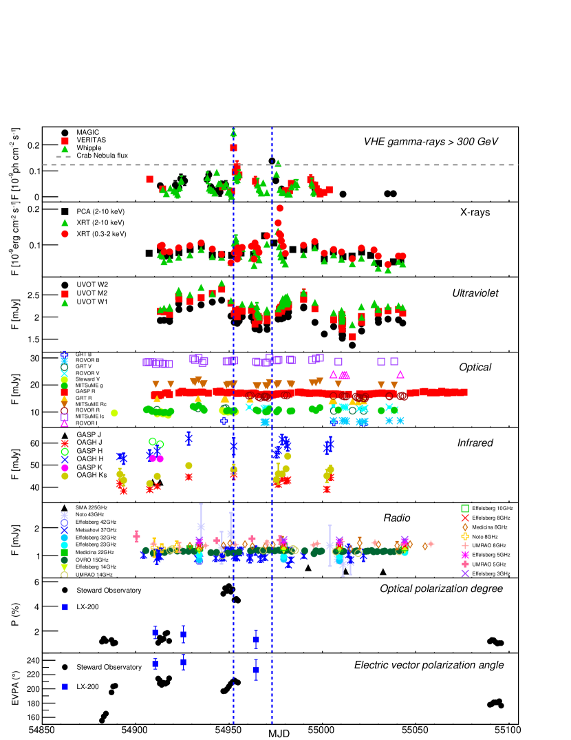
Figure 1: Light curves compiled based on pointing observations in various energy bands. The lowest two panels show measurements of the optical polarization. The two vertical blue lines indicate the location of the two VHE $\gamma$-ray flares at MJD 54952 and MJD 54973 that are discussed in Sect. 4.2 and 4.3.

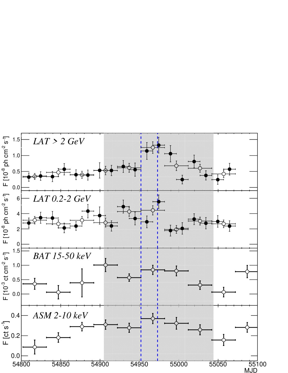
Figure 2: Light curves of instruments with longer integration times. From top to bottom: Fermi-LAT above 2 GeV, Fermi-LAT 0.2-2 GeV, Swift/BAT and RXTE/ASM. Flux points with integration times of 30 days are shown as open markers, while for Fermi-LAT also flux points integrated over 15 days have been derived and are added with filled markers. The grey shaded area depicts the time interval related to the multi-instrument campaign. The two vertical blue lines indicate the location of the two VHE $\gamma$-ray flares at MJD 54952 and MJD 54973 that are discussed in Sect. 4.2 and 4.3.

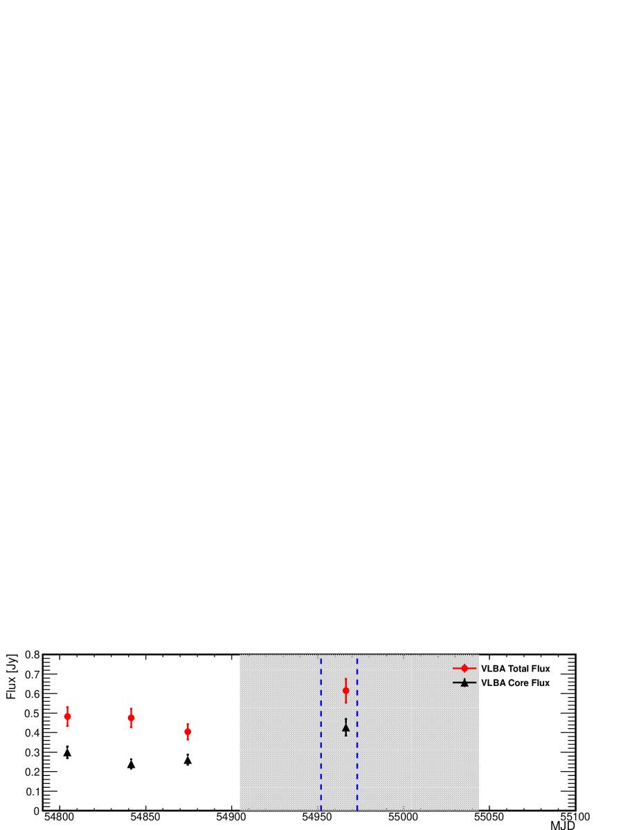
Figure 3: Light curves obtained with the VLBA at 43 GHz. The total flux and the flux from the core region are shown. The grey shaded area depicts the time interval related to the multi-instrument campaign. The two vertical blue lines indicate the location of the two VHE $\gamma$-ray flares at MJD 54952 and MJD 54973 that are discussed in Sect. 4.2 and 4.3.

3.1.1 VHE $\gamma$-ray flaring event starting at MJD 54952

On 2009 May 1, the Whipple 10 m telescope observed Mrk 501 for 2.3 hours and, in the first 0.5 hours (from MJD 54952.35 to MJD 54952.37), detected a VHE flux ($>$300 GeV) increase from $\sim$1.0–1.5 C.U. to $\sim$4.5 C.U., which implies a flux increase by about one order of magnitude with respect to the average VHE flux level recorded during the full campaign. Following the alert by the Whipple 10 m, VERITAS started to observe Mrk 501 after 1.4 hours (at MJD 54952.41) and detected the source at a VHE flux of 1.5 C.U. without statistically significant flux variations during the full observation (from MJD 54952.41 to MJD 54952.48). This VHE flux level was also measured by the Whipple 10 m telescope during approximately the same time window (from MJD 54952.41 to MJD 54952.47), and corresponds to a VHE flux $\sim$4 times larger than the typical flux level of 0.4 C.U. measured during the full campaign. The peak of the flare (which occurred at MJD 54952.37) was caught only by the Whipple 10 m. Still, the Mrk 501 VHE $\gamma$-ray flux remained high for the rest of the night and the following 2 nights (until MJD 54955), which was measured by VERITAS and the Whipple 10 m with very good agreement. Further details about the VERITAS and Whipple 10 m intra-night variability measured on 2009 May 1, as well as the enhanced activity during the first days of May, can be found in Pichel & Paneque (2011) and Aliu et al. (2016).

During the period of the considered VHE $\gamma$-ray flare, no substantial increase in the X-ray regime can be claimed based on the Swift/XRT observations: the 0.3–2 keV and the 2–10 keV fluxes during this flaring episode are about $\sim 8\cdot 10^{-11}$ ergs cm^-2s^-1 and $\sim 1\cdot 10^{-10}$ ergs cm^-2s^-1, which are about $\sim$10% lower and $\sim$30% higher than the average X-ray flux values reported above. However, the Swift/XRT observations started seven hours after the Whipple 10 m and VERITAS observations of this very high VHE state on MJD 54952. The reason for this is that the XRT observations were taken within a ToO activated by the enhanced VHE activity measured by the Whipple 10 m and VERITAS, unlike most of the X-ray pre-planned observations from the MWL campaign which were coordinated with the VHE observations.

In the two lowest panels in Fig. 1, the evolution of the optical polarization degree and orientation are shown. The degree of polarization during the few days around the first VHE flaring activity is measured at 5% compared to a 1% measurement during several observations before and after this flaring activity. Additionally, there is also a rotation of the EVPA by 15 degrees, which comes to a halt at the time of the VHE outburst, when the degree of polarization drops from 5.4% to 4.5% (see further details in Pichel & Paneque, 2011; Aliu et al., 2016).

3.1.2 VHE $\gamma$-ray flaring event starting at MJD 54973

The MAGIC telescope observed Mrk 501 for 1.7 hours on 2009 May 22 (MJD 54973) and measured a flux of 1.2 C.U., which corresponds to $\sim$ 3 times the low flux level. At the next observation on May 24 (MJD 54975.00 to MJD 54975.12), the flux had already decreased to a level of $\sim$0.5 C.U. The Whipple 10 m observed Mrk 501 later on the same date (from MJD 54975.25) and measured a flux of $\sim$0.7 C.U., while the following day (from MJD 54976.23) an measured a flux increase to 1.1 C.U. No VERITAS observations of Mrk 501 took place at this time due to scheduled telescope maintenance.

The MAGIC data of the flaring night were probed for variations on timescales down to minutes, but no significant intra-night variability was found. Moreover, tests for spectral variability within the night in terms of hardness ratios vs. time in different energy bands showed no significant variations either.

Unfortunately, there are no X-ray observations which are strictly simultaneous with the MAGIC observations on MJD 54973. The closest RXTE/PCA observations took place on MJD 56969 and MJD 54974, and the closest Swift/XRT observations are from MJD 54970 and MJD 54976, all of them showing a flux increase (up to a factor of $\sim$2) with respect to the average X-ray flux measured during the campaign.

Under the assumption that no unobserved intra-day variability occurred in the X-ray band, it can be inferred that Mrk 501 was in a state of increased X-ray and VHE activity over a period of up to 5 days. During this period there were no flux changes observed at optical or radio frequencies.

3.2 Spectral variability in individual energy bands

In this section we report on the spectral variability observed during the two few-day long VHE flaring episodes around the peaks of the two SED bumps, namely at X-ray and $\gamma$-rays, where most of the energy is being emitted and where the flux variability is highest.

3.2.1 VHE $\gamma$-rays

The VHE spectra measured with MAGIC and VERITAS, averaged over the entire campaign between 2009 March 15 ((MJD 54905) and 2009 August 1 ((MJD 55044), were reported in Abdo et al. (2011a). Only the time span MJD 54952-54955, where VERITAS recorded VHE flaring activity, had been excluded for the average spectrum and was presented as a separate high-state spectrum (see Fig. 8 of Abdo et al., 2011a). The resulting average spectra relate to a VHE flux of about 0.3 C.U., which is the typical non-flaring VHE flux level of Mrk 501. Additionally, two spectra have been obtained with the Whipple 10 m for that night: a very-high state spectrum, spanning MJD 54952.35-54952.41, which seems to cover the peak of the flare, and a high-state spectrum, derived from the time interval MJD 54952.41 - 54955.00, which is simultaneous with the observations performed with VERITAS. These spectra were reported in Pichel & Paneque (2011), following the general Whipple analysis technique described in Horan et al. (2007), and further details from these spectra are reported in Aliu et al. (2016).

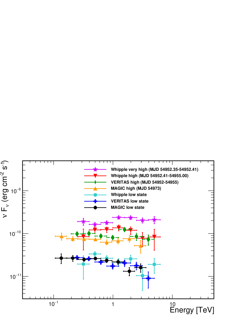
Figure 4: Spectral energy distributions measured by MAGIC, VERITAS and the Whipple 10 m during the low state of the source and two states of increased VHE flux. The spectra have been corrected for EBL absorption using the model of Franceschini et al. (2008).

Table 1: Fit parameters and goodness of fit describing the power-law function for the measured VHE $\gamma$-ray spectra. For low state spectra, the stated flaring time intervals have been excluded from the data. Spectral fits for the Whipple 10 m and VERITAS are listed as presented in Pichel & Paneque (2011).

instrument	flux state	MJD	$F_{0}$ $[10^{-7}$ ph m-2 s-1 TeV${}^{-1}]$	$\Gamma$	$\chi^{2}$ / ndf
Whipple	very-high	54952.35 - 54952.41	$16.1\pm 0.4$	$2.10\pm 0.05$	13.5/8
Whipple	high	54952.41 - 54955	$5.6\pm 0.4$	$2.31\pm 0.11$	3.1/8
VERITAS	high	54952.41 - 54955	$4.17\pm 0.24$	$2.26\pm 0.06$	6.3/5
MAGIC	high	54973	$3.1\pm 0.2$	$2.28\pm 0.06$	1.9/6
Whipple	low	54936 - 54951	$1.16\pm 0.09$	$2.61\pm 0.11$	3.4/8
VERITAS	low	54907 - 55004	$0.88\pm 0.06$	$2.48\pm 0.07$	3.8/5
MAGIC	low	54913 - 55038	$0.93\pm 0.04$	$2.40\pm 0.05$	8.4/6

The re-analysis of the MAGIC data (see Sect. 2), which contains some additional data compared to the analysis presented in Abdo et al. (2011a), revealed a flaring state on MJD 54973, for which a dedicated spectrum was computed. An averaged spectrum was derived based on the remaining data set. The energy distribution of the differential photon flux can be well described by a power-law (PL) function of the form:

$$\frac{dN}{dE}=F_{0}\times\left(E/1\mathrm{TeV}\right)^{-\Gamma},$$ (1)

yielding $F_{0}=\left(9.3\pm 0.4\right)\times 10^{-8}\mathrm{ph}$ $\mathrm{m}^{-2}$ $\mathrm{s}^{-1}$ $\mathrm{TeV}^{-1}$ and $\Gamma=2.40\pm 0.05$. This new MAGIC averaged spectrum was found to be in agreement with the previously presented one, where a power-law fit gave $F_{0}=\left(9.0\pm 0.5\right)\times 10^{-8}\mathrm{ph}$ $\mathrm{m}^{-2}$ $\mathrm{s}^{-1}$ $\mathrm{TeV}^{-1}$ and $\Gamma=2.51\pm 0.05$ (Abdo et al., 2011a). Here we only quote statistical uncertainties of the measurements. The systematic errors affecting data taken by the MAGIC telescope at the time of the presented campaign are discussed in Albert et al. (2008) and are valid for both analyses. They are estimated as an energy scale error of 16%, a systematic error on the flux normalization of 11% and an error on the obtained spectral slope of $\pm 0.2$. In the following, the more recent analysis result will be used.

All the VHE $\gamma$-ray spectra described above are presented in Fig. 4. The spectra displayed in the figure were corrected for absorption by the EBL using the model from Franceschini et al. (2008). Given the proximity of Mrk 501, the impact of the EBL on the spectrum is relatively weak: the attenuation of the flux reaches 50% at an energy of 5 TeV. Many other EBL models (e.g. Finke et al., 2010; Domínguez et al., 2011) provide compatible results at energies below 5 TeV, hence the results do not depend significantly on the EBL model used. The power-law fit parameters (see Eq. 1) of the measured spectra (i.e. non-corrected-for-EBL spectra) can be found in Table 1. For spectra measured with MAGIC, the presented fits also take into account the correlation between the individual spectral points which is introduced by the unfolding of the spectrum, while no explicit unfolding has been applied for the other instruments. The average state spectra measured by the three instruments (after subtracting the time intervals with strong flaring activity in the VHE) agree very well, despite the somewhat different observing periods. This suggests that these VHE spectra are a good representation of the typical VHE spectrum of Mrk 501 during this MWL campaign. The high-state spectra show a spectral slope which is harder compared to the one from the non-flaring state, hence indicating a “harder when brighter” behaviour, as has been reported previously (e.g. Albert et al., 2007a).

3.2.2 GeV $\gamma$-rays

The two few-day long VHE flaring episodes discussed in this paper occurred within the time interval MJD 54952-54982, which is the 30-day time interval with the highest flux and hardest GeV $\gamma$-ray spectrum reported in Abdo et al. (2011a). The flux above 300 MeV F_>300MeV and photon index $\Gamma$ for this 30-day time interval computed using the ScienceTools software package version v9r15p6 and the P6_V3_DIFFUSE instrument response functions, are F${}_{>300\mathrm{MeV}}=(3.6\pm$0.5)$\times$10^-8ph cm^-2s^-1 and $\Gamma=1.64\pm$0.09, while values for the Fermi-LAT spectrum averaged for the entire MWL campaign are F${}_{>300\mathrm{MeV}}=(2.8\pm$0.2)$\times$10^-8ph cm^-2s^-1 and $\Gamma=1.74\pm$0.05 (for further details, see Abdo et al., 2011a). Performing the analysis with the ScienceTools software package version v10r1p1 and the Pass 8 data (which implies somewhat different photon candidate events), as described in Sect. 2, led to a photon flux (above 300 MeV) of F${}_{>300\mathrm{MeV}}=(4.2\pm$0.5)$\times$10^-8ph cm^-2s^-1 and a PL index of $\Gamma=1.68\pm$0.07 for the time interval MJD 54952-54982, and a flux (above 300 MeV) of F${}_{>300\mathrm{MeV}}=(3.0\pm$0.2)$\times$10^-8ph cm^-2s^-1 and a PL index of $\Gamma=1.75\pm$0.04 for the entire campaign. The spectral results derived with Pass 6 and Pass 8 are compatible, and show a marginal increase in the flux and the hardness of the spectra during the time interval MJD 54952-54982 with respect to the full campaign period.

The Pass 8 Fermi-LAT data analysis is more sensitive than the Pass 6 data analysis, and allows us to detect Mrk 501 significantly (TS$>$25) and to determine the spectra around these two flares in time intervals as short as 2 days centered at MJD 54952 and 54973, for the two flares respectively. Additionally, for comparison purposes, we also computed the spectra for 7-day time intervals centered at MJD 54952 and 54973. The Fermi-LAT spectral results for the various time intervals in May 2009 are reported in Table 2. For the first flare, for both the 2-day and 7-day time intervals, the LAT analysis yields a signal with TS$\sim$40. This shows that increasing the time interval from 2 days to 7 days did not increase the $\gamma$-ray signal, and hence indicates that the 2-day time interval centred at MJD 54952 dominates the $\gamma$-ray signal from the 7-day time interval. The spectrum is marginally harder than the average spectrum from the time interval MJD 54952-54982. For the second flare, the 7-day time interval yields a signal significance ($\sim\sqrt{TS}$) 2.6 times larger than that of the 2-day time interval, showing that, contrary to the first flare, increasing the time interval from 2 days to 7 days enhanced the $\gamma$-ray signal considerably. The Fermi-LAT spectrum around the second flare is very similar to the average spectrum obtained for the 30-day time interval MJD 54952-54982.

Table 2: Spectral parameters describing the measured power-law spectra with Fermi-LAT during several temporal intervals in May 2009.

Temporal interval	MJD range	$F_{>300\leavevmode\nobreak\ {\rm MeV}}$ $[10^{-8}$ ph m-2 s${}^{-1}]$	$\Gamma$	TS
May 2009, 30 days	54952 - 54982	$4.2\pm 0.5$	$1.68\pm 0.07$	595
First Flare, 2 days	54951 - 54953	$2.5\pm 1.3$	$1.2\pm 0.3$	43
First Flare, 7 days	54948.5 - 54955.5	$1.7\pm 0.8$	$1.4\pm 0.2$	41
Second Flare, 2 days	54972 - 54974	$4.0\pm 1.7$	$1.8\pm 0.3$	39
Second Flare, 7 days	54969.5 - 54976.5	$5.3\pm 1.0$	$1.6\pm 0.1$	263

For the MWL SEDs presented in Fig. 9, we show the Fermi-LAT spectral results for these two flares performed on three and five differential energy bins (starting from 300 MeV). Here, the shape of the spectrum was fixed to that obtained for the full range for each temporal bin. Upper limits at 95% confidence level were computed whenever the TS value (for the $\gamma$-ray signal of the bin) was below six and/or the uncertainty was equal (or larger) than the energy flux value.

3.2.3 X-rays

In the X-ray band, individual spectra could be derived for each pointing of the two instruments Swift/XRT and RXTE/PCA. Both indicated significant variability in flux and spectral index during the course of the campaign. Fig. 5 shows the XRT and PCA spectra around the times of the first and second flux increase in the VHE range. For the first flare, the variability in flux and spectral shape is larger for XRT than for PCA, but this is mostly due to the fact that many of the XRT observations were performed within a ToO program, and hence they provide a better characterisation of the enhanced activity (see Sect. 2).

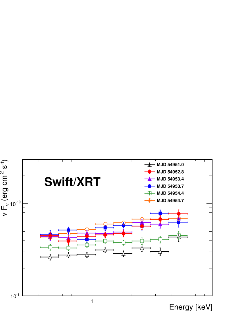
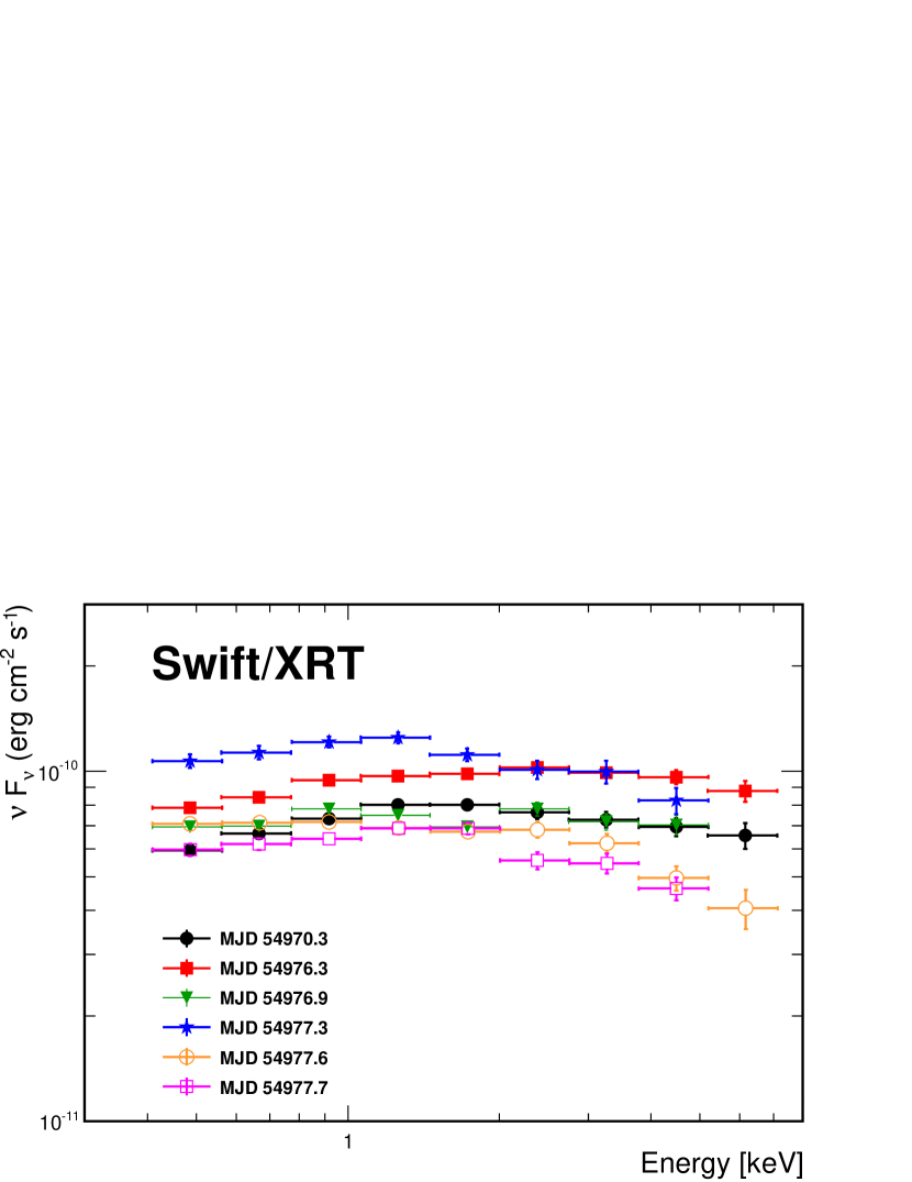
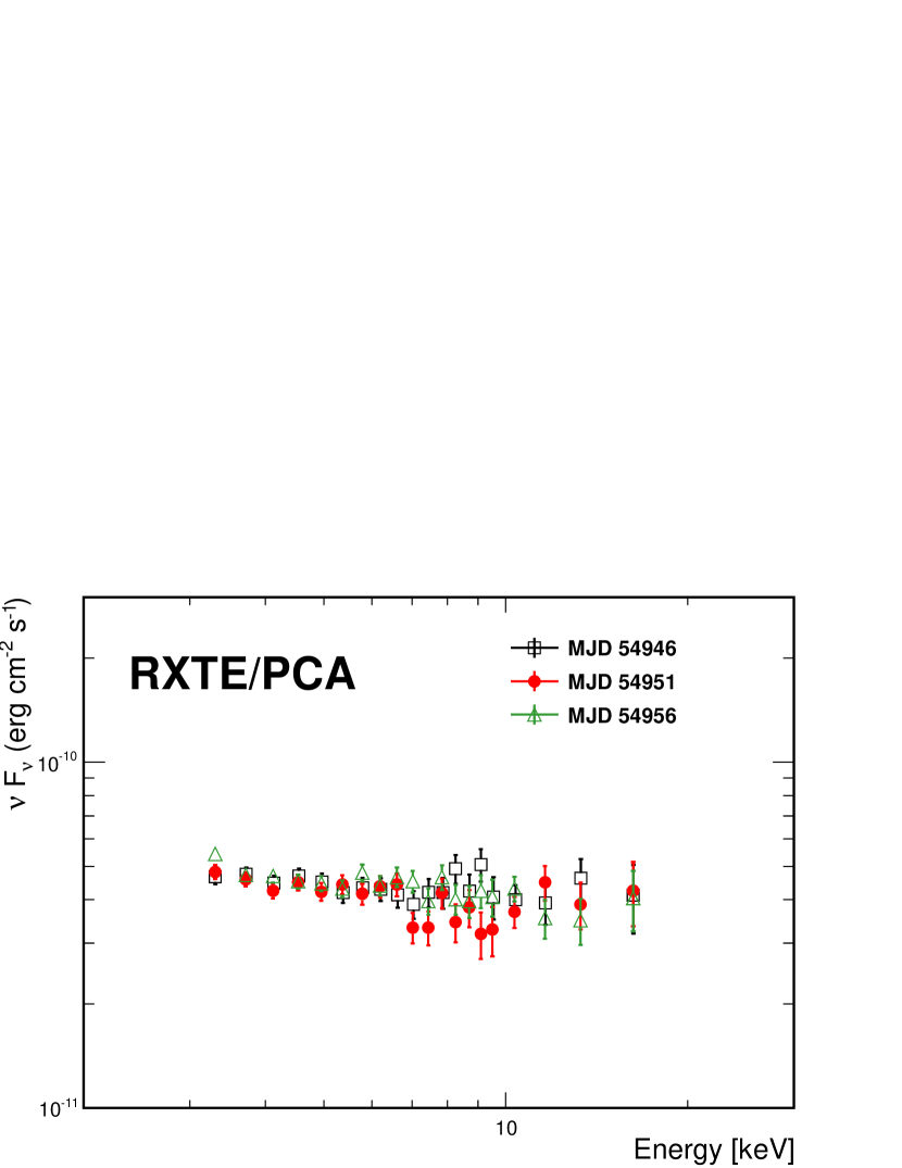
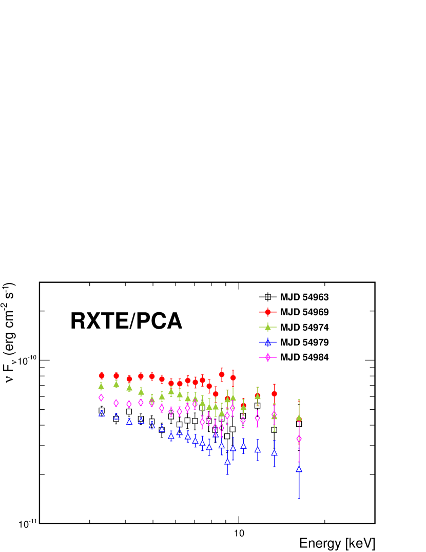
Figure 5: X-ray spectra from single pointings. Left: Swift/XRT. Right: RXTE/PCA. Upper panels: spectra around the first flare (MJD 54952); lower panels: spectra around the second flare (MJD 54973).

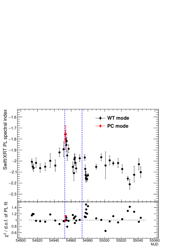
Figure 6: Upper panel: Spectral index obtained from a power-law fit to the Swift/XRT spectra vs. observation date. Lower panel: Reduced $\chi^{2}$ of the power-law fit to the X-ray spectra. The two vertical blue lines indicate the location of the two VHE $\gamma$-ray flares at MJD 54952 and MJD 54973 that are discussed in Sect. 4.2 and 4.3.

Table 3: Spectral results from the power-law (PL) fit to the measured Swift/XRT spectra. For all spectra where the PL fit does not deliver a satisfactory result (fit probability $P<0.3\%\ (3\,\sigma)$), additional results from a log-parabola fit are quoted in the following:                                                                                                                                    MJD 54977.7: $\alpha=2.01_{-0.06}^{+0.05}$, $\beta=0.4_{-0.1}^{+0.1}$, $\chi^{2}$/d.o.f.$=214/163;\quad$ MJD 54978.0: $\alpha=2.05_{-0.03}^{+0.03}$, $\beta=0.32_{-0.06}^{+0.06}$, $\chi^{2}$/d.o.f.$=335/316;$                                                                                                                                    MJD 54980.1: $\alpha=2.03_{-0.02}^{+0.02}$, $\beta=0.312_{-0.05}^{+0.05}$, $\chi^{2}$/d.o.f.$=373/344;\quad$ MJD 55027.6: $\alpha=2.04_{-0.03}^{+0.03}$,$\beta=0.33_{-0.06}^{+0.06}$, $\chi^{2}$/d.o.f.$=293/291.$                                                                                                                                   

MJD	Obs Mode	PL Index	$\chi^{2}$/#d.o.f.
54913.1	WT	$-2.01_{-0.03}^{+0.03}$	246/214
54914.2	WT	$-2.05_{-0.03}^{+0.04}$	246/206
54915.2	WT	$-2.06_{-0.03}^{+0.03}$	200/168
54918.2	WT	$-2.02_{-0.04}^{+0.05}$	130/133
54923.1	WT	$-2.06_{-0.04}^{+0.04}$	160/166
54929.1	WT	$-2.05_{-0.03}^{+0.03}$	179/189
54935.0	WT	$-2.00_{-0.06}^{+0.06}$	88/75
54941.1	WT	$-2.04_{-0.05}^{+0.05}$	111/113
54946.1	WT	$-1.92_{-0.04}^{+0.04}$	139/159
54951.0	WT	$-1.89_{-0.07}^{+0.07}$	62/64
54952.8	PC	$-1.76_{-0.08}^{+0.08}$	56/58
54953.4	PC	$-1.80_{-0.09}^{+0.08}$	57/56
54953.7	PC	$-1.76_{-0.08}^{+0.08}$	66/59
54954.4	WT	$-1.85_{-0.06}^{+0.06}$	84/78
54954.7	WT	$-1.82_{-0.04}^{+0.04}$	165/166
54955.4	WT	$-1.95_{-0.05}^{+0.05}$	100/126
54957.1	WT	$-1.89_{-0.03}^{+0.04}$	163/167
54962.0	WT	$-2.05_{-0.04}^{+0.05}$	125/108
54963.4	WT	$-2.11_{-0.07}^{+0.07}$	79/75
54963.9	WT	$-1.98_{-0.04}^{+0.04}$	140/129
54964.4	WT	$-1.97_{-0.04}^{+0.04}$	141/155
54965.1	WT	$-2.02_{-0.03}^{+0.03}$	269/241

MJD	Obs Mode	PL Index	$\chi^{2}$/#d.o.f.
54966.0	WT	$-2.07_{-0.04}^{+0.04}$	180/183
54970.2	WT	$-1.97_{-0.03}^{+0.03}$	200/199
54976.3	WT	$-1.97_{-0.03}^{+0.03}$	271/244
54976.9	WT	$-2.07_{-0.04}^{+0.04}$	201/184
54977.3	WT	$-2.13_{-0.04}^{+0.04}$	171/139
54977.6	WT	$-2.16_{-0.04}^{+0.04}$	178/162
54977.7	WT	$-2.13_{-0.04}^{+0.04}$	245/164
54978.0	WT	$-2.16_{-0.02}^{+0.02}$	424/317
54979.0	WT	$-2.16_{-0.02}^{+0.02}$	359/298
54980.1	WT	$-2.13_{-0.01}^{+0.02}$	497/345
54989.9	WT	$-2.05_{-0.02}^{+0.02}$	303/287
54995.9	WT	$-1.97_{-0.03}^{+0.03}$	197/196
55001.0	WT	$-2.04_{-0.10}^{+0.10}$	14/21
55006.0	WT	$-1.99_{-0.04}^{+0.04}$	152/159
55010.3	WT	$-2.02_{-0.02}^{+0.02}$	331/295
55015.9	WT	$-2.02_{-0.04}^{+0.04}$	147/158
55020.9	WT	$-2.07_{-0.04}^{+0.04}$	180/175
55027.6	WT	$-2.16_{-0.02}^{+0.02}$	377/292
55029.9	WT	$-2.21_{-0.04}^{+0.04}$	144/101
55035.2	WT	$-2.12_{-0.07}^{+0.08}$	89/70
55040.8	WT	$-2.03_{-0.05}^{+0.05}$	101/107
55043.0	WT	$-2.10_{-0.05}^{+0.05}$	109/102

Around the first VHE flare, the XRT spectra tend to be much harder and appear to show an upward curvature towards higher energies. The hardening of the spectrum is confirmed by a spectral analysis performed using a power-law spectral model with the hydrogen density $N_{H}$ fixed to the Galactic value. Fig. 6 shows the spectral index light curve (see also Table 3) and the reduced $\chi^{2}$ of the individual fits. Based on the reduced $\chi^{2}$ values, the representation by a simple power-law function is sufficient for most spectra. Around MJD 54952-54953, which roughly corresponds to the time of the first VHE flare, a peak in the hardness of the spectrum can be seen.

Around the second flux increase in the VHE $\gamma$-ray band, variability was seen by both Swift/XRT and RXTE/PCA, with flux changes by up to a factor of 2 with respect to the flux average of $\sim$(7–8)$\cdot 10^{-11}$ ergs cm^-2s^-1 in the 2–10 keV band (see Fig. 1). However, no particular hardening of the spectrum was found (see Fig.6), as observed for the first flare.

3.3 Quantification of the multi-instrument variability

As a quantitative study of the underlying variability seen at different wave-bands, the fractional variability $F_{\text{var}}$ has been determined for each instrument according to Eq. 10 in Vaughan et al. (2003):

$$F_{\text{var}}=\sqrt{\frac{S^{2}-<\sigma^{2}_{\text{err}}>}{<F_{\gamma}>^{2}}},$$ (2)

where $S^{2}$ represents the variance, $<\sigma^{2}_{\text{err}}>$ specifies the mean square error stemming from measurement uncertainties and ${<F_{\gamma}>}$ is the arithmetic mean of the measured flux. The term under the square root is also known as the normalised excess variance $\sigma^{2}_{\text{NXS}}$.

The uncertainty of $F_{\text{var}}$ is calculated following the prescription from Poutanen et al. (2008), as described in Aleksić et al. (2015a), so that they are valid also in the case when $\Delta F_{\text{var}}\ll F_{\text{var}}$:

$$\Delta F_{\text{var}}=\sqrt{F^{2}_{\text{var}}+err(\sigma^{2}_{\text{NXS}})}-F_{\text{var}},$$ (3)

with the error of the normalised excess variance $err(\sigma^{2}_{\text{NXS}})$ as defined in Eq. 11 in Vaughan et al. (2003).

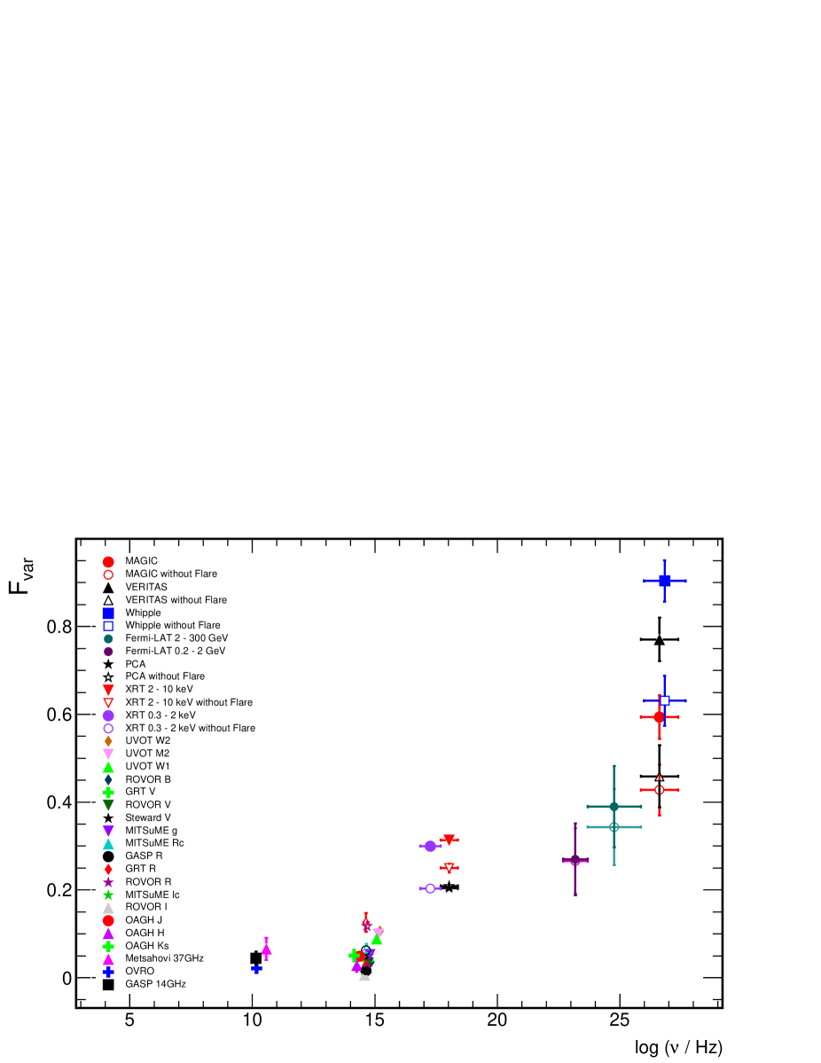
Figure 7: Fractional variability at different frequencies. All the $F_{\text{var}}$ values are computed with the single observations reported in Fig. 1, with the exception of the $F_{\text{var}}$ values related to Fermi-LAT which were computed with 15-day and 30-day time intervals, and depicted with full circles and open light-coloured circles respectively. Open symbols for optical bands indicate the fractional variability after subtracting the host galaxy contribution, as determined in Nilsson et al. (2007). For the X-ray and the VHE $\gamma$-ray band, open markers depict the variability after removal of flaring episodes from the light curves as described in the text.

This methodology to quantify the variability has the caveat that the resulting $F_{\text{var}}$ and related uncertainty depend very much on instrument sensitivity and the observing sampling, which is different for the different energy bands. In other words, a densely sampled light curve with small uncertainties in the flux measurements may allow us to see flux variations that are hidden otherwise, and hence may yield a larger $F_{\text{var}}$ and/or smaller uncertainties in the calculated values of $F_{\text{var}}$. Some practical issues in the application of this methodology in the context of multiwavelength campaigns are elaborated in Aleksić et al. (2014, 2015b, 2015a).

For Swift/XRT and RXTE/PCA in the X-ray band, and MAGIC, VERITAS and the Whipple 10 m in the VHE regime, the fractional variability has been calculated for the full dataset and also after removal of the temporal intervals related to the two flaring episodes (MJD 54952-54955, MJD 54973-54978). The fractional variability specifically computed for the period around the first flaring episode has been recently reported in Aliu et al. (2016). For measurements in the optical R band, $F_{\text{var}}$ has additionally been calculated for optical fluxes corrected for the host galaxy emission as derived in Nilsson et al. (2007). For datasets containing fewer than five data points, no $F_{\text{var}}$ was calculated. The results are presented in Fig. 7.

A negative excess variance was obtained for datasets from the following instruments: UMRAO (at 5 GHz and 8 GHz), Noto (at 8 GHz and 43 GHz), Medicina (at 8 GHz), Effelsberg (all bands) and the near-IR measurements within the GASP-WEBT program (all bands). Such a negative excess variance is interpreted as an absence of flux variability within the sensitivity range of the instrument. These datasets have not been included in Fig. 7.

At low frequencies, from radio to optical, no substantial variability was detected, with $F_{\text{var}}$ ranging from $\approx 0.02-0.06$ in radio to $0.01-0.1$ in optical. In the X-ray band, we find $F_{\text{var}}\approx 0.3$, indicating substantial variation in the flux during the probed time interval. After removal of the flaring times, variabilities of $F_{\text{var}}\approx 0.2-0.25$ are still seen. The fractional variability in the $\gamma$-ray band covered by Fermi-LAT is of the order $F_{\text{var}}\approx 0.3-0.4$; yet the Fermi-LAT $F_{\text{var}}$ values are not directly comparable to the other instruments, as GeV variability on day timescales, which could be higher than that computed (separately) for the 15-day and the 30-day timescales, cannot be probed. Strong variability can be noted at VHE, with $F_{\text{var}}\geq 0.4$ for the datasets without the flares, and $F_{\text{var}}\geq 0.6$ (0.9 for Whipple 10 m) for observations including the flaring episodes.

All in all, Mrk 501 showed a large increase in variability with increasing energy, ranging from an almost steady behaviour at the lowest frequencies to the highest variability observed in the VHE band.

3.4 Multi-instrument correlations

To study possible cross-correlations of flux changes between the different wavelengths, we determined the discrete correlation functions (DCF), following Edelson & Krolik (1988), based on the light curves obtained by the various instruments. The DCF allows a search for correlations with possible time lags, which could result e.g. from a spatial separation of different emission regions. We probed time lags in steps of 5 days up to a maximum shift of 65 days. The step size corresponds to the overall sampling of the light curve and thus to the objective of the MWL campaign itself, which was to probe the source activity and spectral distribution every $\approx 5$ days. The maximum time span is governed by the duration of the campaign, as a good fraction of the light curve should be available for the calculation of cross-correlations. We chose a maximum of 65 days, which corresponds to roughly half the time span of the entire campaign. Because of the uneven sampling and varying exposure times, the significance of the correlations derived from the prescription given in Edelson & Krolik (1988) might be overestimated (Uttley et al., 2003). We derived an independent assessment of the significance of the correlation by means of dedicated Monte Carlo simulations as described in Arévalo et al. (2009) and Aleksić et al. (2015b, a).

In this study, possible cross-correlations between instruments of different wave-bands were examined. As already suggested by the low level of variability in the radio and optical band throughout the campaign, no correlations with any other wave-band were found for these instruments. A correlation with flux changes in the MeV-GeV range could not be probed on timescales of days due to the integration time of 15–30 days required by Fermi-LAT for a significant detection. A similar situation occurs in the X-ray bands from Swift/BAT and RXTE/ASM, which also need integration times of the same order, and are thus also neglected for day-scale correlation studies.

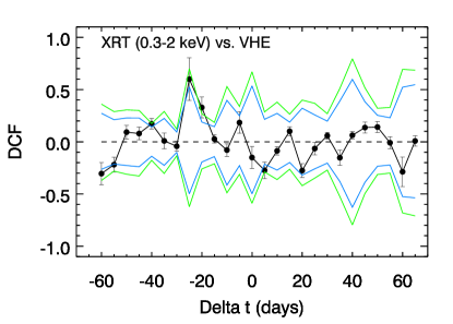
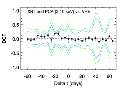
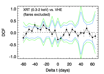
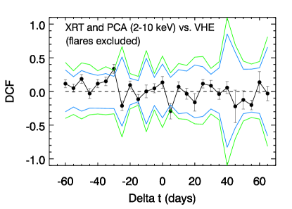
Figure 8: DCF derived for VHE $\gamma$-rays (combined from MAGIC, VERITAS and Whipple measurements) and two X-ray bands (Swift/XRT measurements within the 0.3 - 2 keV band; Swift/XRT and RXTE/PCA combined within the 2 - 10 keV band). The blue (green) lines depict the 95% (99%) confidence intervals derived from Monte Carlo generated light curves (see text for detailed explanation). Left: DCF of complete datasets. Right: DCF derived with the datasets after subtracting the two flaring periods (excluded time windows as explained in the text).

Therefore, the study focuses on the highly sensitive X-ray and VHE $\gamma$-ray observations, namely the ones performed with Swift/XRT, RXTE/PCA, MAGIC, VERITAS and Whipple 10 m, which are also the ones that report the highest variability, as shown in Fig. 7. In the VHE $\gamma$-ray band, the number of observations is relatively small (in comparison to the number of X-ray observations performed with Swift and RXTE), and hence we compile a single light curve with a dense temporal sampling of Mrk 501, including the measured flux points from all three participating VHE $\gamma$-ray telescopes. This procedure is straight-forward, as VERITAS and MAGIC both measured the flux above 300 GeV and the Whipple 10 m measurements have been scaled to report a flux in the same energy range (see Sect. 2). We also combined measurements by Swift/XRT in the 2-10 keV band and data points from RXTE/PCA to a single light curve, as the same energy range is covered by the two instruments. The light curve in the 0.3-2 keV band consists of only measurements performed by Swift/XRT. The DCF vs. time-shift distributions for the two X-ray bands and the VHE $\gamma$-ray measurements are shown on the left hand side of Fig. 8.

At a time lag $\Delta$T$=\left(\text{T}_{\text{VHE}}-\text{T}_{\text{X-ray}}\right)$ on the order of -20 to -25 days, a hint of correlation at the level of 2 sigma between fluxes in the soft X-ray band and the VHE $\gamma$-ray band is seen in the top left panel of Fig. 8. This feature is dominated by the two flaring events, as the dominant flare in VHE $\gamma$-rays occured around MJD 54952, while the largest flux increase in soft X-rays was seen around MJD 54977, with a separation of $24-25$ days. The right hand side of Fig. 8 reports the evaluation of the correlations after the flaring episodes have been excluded from the X-ray and VHE $\gamma$-ray light curves. The above-mentioned feature at 20-25 days is no longer present.

The large growth of the confidence intervals apparent at time shifts of $\Delta$T $\approx 40$ days are caused by sparsely populated regions in the VHE $\gamma$-ray light curve, mainly towards the end of the campaign. In case the light curves are shifted by $\approx 40$ days with respect to each other, these regions overlap with densely populated regions in the X-ray light curves, which results in a larger uncertainty of the determined DCF.

Overall, no significant correlation between X-ray and VHE $\gamma$-ray fluxes is found for any of the combinations probed.

4 Evolution of the spectral energy distribution

The time-averaged broadband SED measured during this MWL campaign (from MJD 54905 to MJD 55044) was reported and modeled satisfactorily in the context of a one-zone synchrotron self-Compton (SSC) scenario (Abdo et al., 2011a). In such a model, several properties of the emission region are defined, such as the size of the region $R$, the local magnetic field $B$ and the Doppler factor $\delta$, which describes the relativistic beaming of the emission towards the observer. Furthermore, the radiating electron population is described by a local particle density $n_{e}$ and the spectral shape. For the averaged data set of this campaign, the underlying spectrum of the electron population was parameterized with a power-law distribution from a minimum energy $\gamma_{\text{min}}$ to a maximum energy $\gamma_{\text{max}}$, with two spectral breaks $\gamma_{\text{break,1}}$ and $\gamma_{\text{break,2}}$. The two breaks in the electron energy distribution (EED) were required in order to properly model the entire broadband SED. Because of the relatively small multiband variability during the 4.5-month long observing campaign (once the first VHE flare is removed) and the large number of observations performed with all the instruments, the average SED could be regarded as a high-quality representation of the typical broadband emission of Mrk 501 during the time interval covered by the campaign, and hence the one-zone SSC model was constrained to describe all the data points (including 230 GHz SMA and interferometric 43 GHz VLBA observations).

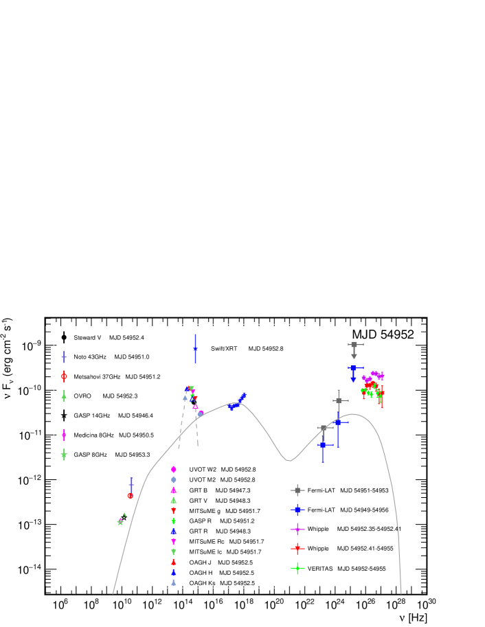
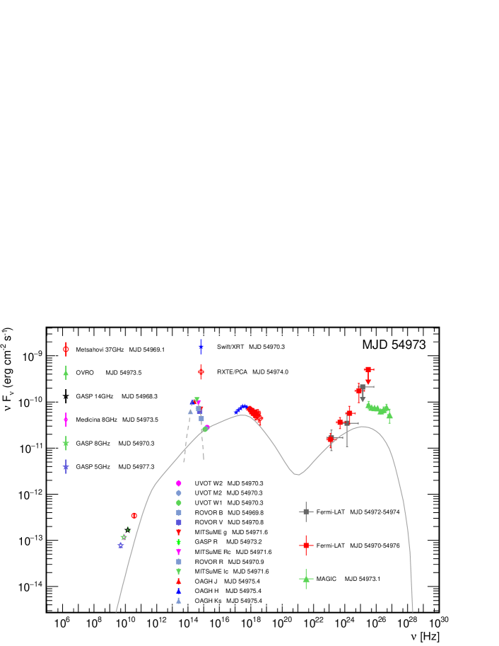
Figure 9: Broadband SED of Mrk 501 during the two VHE high states observed within the campaign (upper panel: MJD 54952, lower panel: MJD 54973). See text for details regarding the included spectral measurements. The data points have been corrected for EBL absorption according to the model by Franceschini et al. (2008). The emission of the host galaxy parameterized according to Silva et al. (1998) is shown with a grey dashed line, while the one-zone SSC model describing the average broadband SED over the entire campaign (see Abdo et al., 2011a) is depicted with a grey solid line.

In this work, we focus on the characterization of the broadband SED during the two flaring episodes occurring in May 2009. As reported in Sect. 3.1, these two flaring episodes start on MJD 54952 and MJD 54973, and last for approximately three and five days each, respectively. There is some flux and spectral variability throughout these two flaring episodes, but for the sake of simplicity, in this section we will attempt to model only the SEDs related to the VHE flares on MJD 54952 and 54973, which are the first days of these two flaring activities. We try to model these two SEDs with the simplest leptonic scenarios, namely a one-zone SSC and a two-independent-zone SSC model. In the latter we assume that the quiescent or slowly changing emission is dominated by one region that is described by the SSC model parameters used for the average/typical broadband emission from the campaign (see Abdo et al., 2011a), while the flaring emission (essentially only visible in the X-ray and $\gamma$-ray bands) is dominated by a second, independent and spatially separated region.

The assumption of a theoretical scenario consisting of one (or two) steady-state homogenous emission zone(s) could be an oversimplification of the real situation. The blazar emission may be produced in inhomogeneous regions, involving stratification of the emitting plasma both along and across a relativistic outflow, and the broad-band SED may be the superposition of the emission from all these different regions, characterized by different parameters and emission properties, as reported by various authors (e.g. Ghisellini et al., 2005; Graff et al., 2008; Giannios et al., 2009; Chen et al., 2011; Zhang et al., 2014; Chen et al., 2015). In this paper we decided to continue using the same theoretical scenario used in Abdo et al. (2011a), which we adopted as the reference paper for this dataset. We also kept the discussion of the model parameters at a basic level, and did not attempt to perform any profound study of the implications of those parameters.

In this work we used the SSC model code described in Takami (2011), which is qualitatively the same as the one used in Abdo et al. (2011a), with the difference that the EED is parameterized as

$$\frac{dN}{d\gamma}=\cases{n}_{e}\cdot\gamma^{-\alpha_{1}},&(\gamma_{\text{min}}<\gamma<\gamma_{\text{break},1})\\ n_{e}\cdot\gamma_{\text{break},1}^{\alpha_{2}-\alpha_{1}}\cdot\gamma^{-\alpha_{2}},(\gamma_{\text{break},1}<\gamma<\gamma_{\text{break},2})\\ n_{e}\cdot\gamma_{\text{break},1}^{\alpha_{2}-\alpha_{1}}\cdot\gamma_{\text{break},2}^{\alpha_{3}-\alpha_{2}}\cdot e^{\left(\frac{\gamma_{\text{break},2}}{\gamma_{\text{max}}}\right)}\\ \;\;\;\;\;\cdot\gamma^{-\alpha_{3}}\cdot e^{\left(-\frac{\gamma}{\gamma_{\text{max}}}\right)}(\gamma_{\text{break},2}<\gamma),{}$$ (4)

where $n_{e}$ is the electron number density. For reasons of comparability, only this definition is applied in all the SED modelling results in this section, including that of the quiescent, averaged SED obtained over the full MWL campaign. The corresponding one-zone SSC model parameter values defining the averaged SED from the full 2009 multi-instrument campaign are listed in Table 4. The parameter values are identical to those from the “Main SSC fit” reported in Table 2 of Abdo et al. (2011a), with the only difference being the usage of the electron number density $n_{e}$, instead of the equipartition parameter. The contribution of star light from the host galaxy can be approximately described with the template from Silva et al. (1998), as was done in Abdo et al. (2011a).

Table 4: SSC model parameters which characterize the average emission over the entire MWL campaign. The parameters apply to a one-zone model defined by Eq. 4 and are retrieved from the modelling presented in Abdo et al. (2011a).

	$\gamma_{\text{min}}$	$\gamma_{\text{max}}$	$\gamma_{\text{break},1}$	$\gamma_{\text{break},2}$	$\alpha_{1}$	$\alpha_{2}$	$\alpha_{3}$	ne	B/mG	$\log(\frac{R}{cm})$	$\delta$
av. state	600	$1.5\times 10^{7}$	$4\times 10^{4}$	$9\times 10^{5}$	2.2	2.7	3.65	635	15	$17.11$	12

For the characterization of the SEDs collected during the two flaring states, we allow for an EED with two spectral breaks in the case of one-zone SSC models. For the second zone in the two-zone SSC scenario, we keep the somewhat simpler description of the electron energy distribution as a power law with only one spectral break (i.e. $\alpha_{2}\equiv\alpha_{1}$ in Eq. 4).

4.1 The grid-scan strategy for modeling the SED

In contrast to the commonly used method of adjusting the model curve to the measured SED data points (e.g. Tavecchio et al., 1998, 2001; Albert et al., 2007a), in this study we applied a novel variation on the grid-scan approach in the space of model parameters. Given a particular theoretical scenario (e.g. the one-zone or two-zone SSC model), we make a multi-dimensional grid with the $N$ model parameters that we want to sample. For each parameter, we define a range of allowed values and a step size for the variation within this range. Theoretical (SSC) model curves are calculated for each point on the grid, i.e. for each combination of the $N$ parameter values. Subsequently, the goodness of the resulting model curves in reconstructing the data points is quantified by means of the $\chi^{2}$ between data and model, which takes into account the statistical uncertainties of the individual measurements. At the moment, systematic uncertainties are not considered for the evaluation of the agreement. This would require performing the entire procedure for various shifts in the flux and energy scale for each instrument, as well as for possible distortions in the individual spectra. The net impact of including systematic uncertainties in the single-instrument spectra would be a larger tolerance for the agreement between the experimental data and the theoretical model curves, which would yield a larger degeneracy in the parameter values that can model the data. While this will be investigated in the future, it is beyond the scope of this paper. Therefore, the data-model agreements reported in this manuscript, which are based on the $\chi^{2}$ analysis using only the statistical uncertainties, provide a lower limit to the actual agreement between the presented experimental data and the theoretical model curves being tested, and we mostly use them to judge the relative agreement of the various theoretical model curves.

Depending on the complexity of the model itself, the model calculations for an entire grid can be very intensive in computing power. For instance, one of the simplest SSC scenarios, involving only one emission zone with an electron energy distribution with one spectral break, already leads to a grid spanning a nine-dimensional parameter space. With the ranges and grid spacings we are using in this work, the number of model curves to calculate and evaluate amounts to tens of million. For this reason, the access to cluster computing becomes essential for this grid-scan modelling approach. The model calculations in this work have been performed using the computing farms at SLAC and TU Dortmund.

After the evaluation of all models regarding their level of agreement with the data, individual models can be chosen for the final set, according to the achieved probability of agreement (derived from the $\chi^{2}$ and the number of degrees of freedom). These sets of models can then be visualized both in the SED representation and in the space of parameter values defining the models, which could populate non-continuous regions in the parameter space.

One aim of the grid-scan strategy is to keep the range of model parameters as wide as possible. By sampling a large parameter phase space we can reduce the bias which is usually introduced into the modelling by adopting a set of assumptions or educated choices. Another advantage is the fact that, besides the obvious aim of finding parameter values which describe the data in the best way, the “grid-scan” approach also offers the possibility of investigating the degeneracy of the model-to-data agreement regarding each individual model parameter. In order to do this, sets of models within bands of achieved fit probabilities are compiled and their distributions in each of the model parameters are visualized. Based on such plots, interesting regions in the parameter space can be selected for a deeper search, which leads to models with an even better agreement with the data and to a more thorough study of the degeneracy of individual model parameters. Finally, the grid-scan method allows one to potentially find multiple clusters or regions in the model parameter phase space that could be related to different physical scenarios, which can be equally applicable to the data set at hand, but might be missed by statistical methods aiming at only ”one best” solution.

A concept for “grid-scan” SED modelling has already been presented in Cerruti et al. (2013), where model curves are computed for each point on the parameter space grid, but the assessment of the agreement between model and data is performed in a different way: the authors evaluate the agreement based on seven observables (i.e. the frequency and luminosity of the synchrotron peak, the measured X-ray spectral slope and the GeV and TeV spectral slopes and flux normalizations), which are derived from the model curves and compared to the data. They also provide a family of solutions, involving any uncertainties in the observables. In the work presented here, the model-to-data agreement criterion, which is used to select a set of models, is derived directly from the $\chi^{2}$-distances between each data point and each model curve, without computing any secondary characteristics of the SED which may introduce additional uncertainties. Cerruti et al. (2013) also determine this distance for the models picked by their algorithm, but apply it only as a posteriori check of their result. Furthermore, the authors have reduced the dimensionality of the parameter space from nine to six, and used only five steps for each parameter, which implied the creation of a grid with $5^{6}$=15625 SED realizations. In the work presented here, the smallest grid-scan implied the creation of more than $40\times 10^{6}$ SED realizations. Additionally, after selecting interesting regions in the various model parameters with the grid-scan, we went one step further and performed a second (dense) grid-scan focused only on those regions, and using a smaller step size.

The objective of finding uncertainty ranges of model parameters has also been addressed by Mankuzhiyil et al. (2011); Zabalza (2015). Here, a Markov-Chain Monte Carlo procedure is used to fit emission model curves (for a number of different emission models) to the observational results. While this approach delivers uncertainties or probability distribution functions for the particle distribution parameters, this is done only for one particular solution. Disjointed regions of equally good model configurations, i.e. “holes” in the probability distribution for the individual parameters, are not found following this method.

A 3-dimensional parameter grid with 9504 (48$\times$22$\times$9) steps was used by Petry et al. (2000) to find the most suited model parameter set to describe weekly averaged SEDs of Mrk 501, where the ”best” model was selected as the one with the smallest data-model difference, quantified with a $\chi^{2}$ approach. Despite the usage of a parameter grid, the goal and merits of that work differ from those of the methodology presented here. While Petry et al. (2000) used the 3-dimensional parameter grid to find the best model (as in Mankuzhiyil et al., 2011, with a $\chi 2$ minimization procedure), in this work the 9-dimensional grid is used to find the family (or families) of parameter values that give a good representation of the broad-band SED, and to show the large degeneracy of the model parameters to describe the SED.

Table 5: Grid of SSC model parameters which is probed for one-zone models within the coarse grid-scan. For each parameter the probed range is given by a minimum and maximum value, and the number of tested values is given by the number of steps between (and including) these limits. The number of SSC models required to realize this grid-scan amounts to 62 million.

coarse grid
one-zone	$\gamma_{\text{min}}$	$\gamma_{\text{max}}$	$\gamma_{\text{break},1}$	$\gamma_{\text{break},2}$	$\alpha_{1}$	$\alpha_{2}$	$\alpha_{3}$	ne	B/mG	$\log(\frac{R}{cm})$	$\delta$
min	$1\times 10^{2}$	$1\times 10^{6}$	$1\times 10^{4}$	$1\times 10^{5}$	1.7	2.1	3.6	$1\times 10^{3}$	5	14.0	1
max	$1\times 10^{4}$	$1\times 10^{8}$	$1\times 10^{5}$	$3.2\times 10^{6}$	2.3	3.3	4.8	$1\times 10^{6}$	250	16.0	60
$\#$ of steps	3	3	4	4	7	7	4	7	9	5	7
spacing	log	log	log	log	lin	lin	lin	log	log	lin	log

Table 6: Grid of SSC model parameters which is probed for two-zone models within the coarse grid-scan. In two-zone models only the second zone is defined by the parameters given here, while the first zone is given by the model derived in Abdo et al. (2011a), and reported in Table 4. The number of SSC models required to realize this grid-scan amounts to 40 million.

coarse grid
two-zone	$\gamma_{\text{min}}$	$\gamma_{\text{max}}$	$\gamma_{\text{break}}$	$\alpha_{1}$	$\alpha_{2}$	ne	B/mG	$\log(\frac{R}{cm})$	$\delta$
min	$1\times 10^{2}$	$1\times 10^{5}$	$1\times 10^{4}$	1.7	2.0	100	5	14.0	1
max	$1\times 10^{6}$	$1\times 10^{8}$	$1\times 10^{7}$	2.3	4.8	$1\times 10^{6}$	250	18.0	60
$\#$ of steps	5	4	7	7	8	9	9	9	7
spacing	log	log	log	lin	lin	log	log	lin	log

For the theoretical SED modelling of the two flaring states of Mrk 501, following the grid-scan strategy outlined above, the parameter ranges given in Table 5 and Table 6 have been investigated for the one-zone and two-zone scenarios described at the beginning of this section. Given that we aim to sample a wide range of parameter values with a relatively coarse step (for each parameter), we denote these scans as “coarse grid-scans”. The general orientation for the choice of parameter ranges is based on previous works on modelling of the SED of Mrk 501, e.g. Albert et al. (2007a); Anderhub et al. (2009); Abdo et al. (2011a); Mankuzhiyil et al. (2012). Based on these values, one-zone SSC models have been built as well as second zones for the two-zone scenario. In the latter, the first zone is described by the model reproducing the average emission seen over the entire campaign (see Abdo et al., 2011a), while only the second zone is varied as described by the model parameters from the grid presented here. One could reduce the phase space of the grid-scan by imposing certain relations between the locations of the breaks ($\gamma_{\text{break}}$) in the EED and the size $R$ and magnetic field $B$ values, as well as to constrain the index values before and after the breaks (e.g. $\Delta\alpha=1$). But cooling breaks with a spectral change twice larger than the canonical value of 1 were necessary to describe the broadband SED of Mrk 421 within a SSC homogeneous model scenario (see Sect. 7.1 of Abdo et al., 2011b), and the breaks needed by the SSC models are not always related to the cooling of the electrons, but instead could be related to the acceleration mechanism, as reported for Mrk 501 in Abdo et al. (2011a). Internal breaks (related to the electron acceleration) have been reported for various blazars (e.g. Abdo et al., 2009; Abdo et al., 2010a). The origin of these internal breaks, as well as large spectral changes at the EED breaks, may be related to variations in the global field orientation, turbulence levels sampled by particles of different energy, or gradients in the physical quantities describing the system. These characteristics are not taken into account in the ”relatively simple” homogenous SSC models, and argue for more sophisticated theoretical scenarios, such as the ones mentioned above. In order to keep the range of allowed model parameter values as broad as possible, in this exercise we did not impose constraints on the location of the EED breaks or in the index values before/after the breaks. The hardest index we use in this study is 1.7, which is harder than the canonical index values $>2$ derived from shock acceleration mechanisms and used very often to parameterize the broad-band SEDs of blazars. But this is actually not a problem, as various authors have shown that indices as hard as 1.5 can be produced through stochastic acceleration (e.g. Virtanen & Vainio, 2005), or through diffusive acceleration in relativistic magnetohydrodynamic shocks, as reported in Stecker et al. (2007); Summerlin & Baring (2012); Baring et al. (2016). We also use $\gamma_{\text{min}}$ values extending up to $10^{6}$, which are substantially higher that those used in conventional SSC models (that go typically up to $\sim 10^{3}$); but such high $\gamma_{\text{min}}$ values have also been used already by various authors (e.g. Katarzyński et al., 2006; Tavecchio et al., 2009; Lefa et al., 2011a, b).

In the evaluation of the models, we used two additional constraints, besides the requirement of presenting a good agreement with the SED data points. Equipartition arguments impose the condition that the energy densities held by the electron population ($u_{e}$) and the magnetic field ($u_{B}$) should be of comparable order. Typically, the parameterization of the broadband SED of Mrk501 (and all TeV blazars, in general) within SSC theoretical scenarios require $u_{e}\sim 10^{2-3}u_{B}$, which implies higher energy in the particles than in the magnetic field, at least locally, where the broadband blazar emission is produced (see e.g. Tavecchio et al., 2001; Abdo et al., 2011a; Aleksić et al., 2015b). There is no physical reason for any specific (somewhat arbitrary) cut value in the quantity $u_{e}/u_{B}$, but driven by previous works in the literature, in this study we only consider models fulfilling the requirement of $u_{e}/u_{B}<10^{3}$. Secondly, the observed variability timescales have to be taken into account. Following causality arguments, the observed variability should not happen on timescales which are shorter than the time needed to distribute information throughout the emitting region. Based on the given Doppler factor $\delta$ and the size of the emitting region $R$, the implied minimum variability timescale quantity for each model is derived according to

$$t_{\text{var}_{\text{min}}}\simeq\frac{\left(1+z\right)R}{\delta c}.$$ (5)

While for the first flare we observed large (up to factors of $\sim$4) flux changes within 0.5 hour (Pichel & Paneque, 2011; Aliu et al., 2016), the second flare shows substantial flux changes ($\sim$2) on timescales of several days. Consequently, we consider only models which yield a minimum variability timescale of $t_{\text{var}_{\text{min}}}\leq 0.25$ hours and $t_{\text{var}_{\text{min}}}\leq 1$ day for the 1st and 2nd VHE flare, respectively.

4.2 1st VHE flare

All spectral points which were obtained at the time or close to the time of the VHE flare measured by VERITAS and the Whipple 10 m telescope at MJD 54952 are shown in the top panel of Fig. 9 (see Sect. 3.1.1 and 3.1.1 for details on the individual observation times).

The attempt to apply the grid-scan to the broadband SED from this flaring episode is affected by the fact that some of the flux variations occurred on sub-hour timescales, and the observations performed were not strictly simultaneous as discussed in the previous sections. Therefore, the SED reported in this section is not necessarily a good representation of the true SED for this flaring episode, and hence any modelling results have to be regarded as inconclusive.

In this SED modeling exercise, the data used are the measurements from Swift (UV and X-rays), Fermi-LAT (2-day spectrum) and Whipple 10 m very-high state. The optical and infrared, as well as the radio points, are not taken into account for the evaluation of the agreement of the SSC model curves with the data. The former two are strongly dominated by emission from the host galaxy, and the latter only serve as upper limits for the SSC flux, as the radio emission shows substantially lower variability timescales and is widely assumed to stem from a larger region than the emitting blob responsible for a few-day long flaring activity.

Exploiting the entire parameter grid space, neither the one-zone SSC model nor the two-zone SSC model can reconstruct the measured broadband SED, with the data-model agreement quantified with $\chi^{2}/d.o.f.>300/20$, which would imply a probability of agreement $P$ (or p-value) between the SSC model curves and the data points of $P<10^{-50}$. When removing the tight constraint given by the cut in $t_{\text{var}_{\text{min}}}$, the best agreement obtained with the one-zone SSC scenario from the grid-scan defined by Table 5 is $\chi^{2}/d.o.f.=180/20$ ($P\sim 10^{-27}$). The two-zone scenario with the quiescent emission characterized by the model parameters from the average SED reported in Table 4 and the (spatially independent) region responsible for the flaring activity modeled based on the coarse grid parameter values reported in Table 6 provides at best an agreement given by $\chi^{2}/d.o.f.=225/20$ ($P\sim 10^{-36}$). Since the X-ray spectrum at low energies is already accounted for with the “quiescent” zone, the contribution from the “flaring” zone (which is needed to explain the increase in the flux at VHE) exceeds the measured flux at X-ray energies, and hence yields a bad agreement with the data points.

Besides trying with the grid-scan defined in Table 5, we also evaluated the model-to-data agreement when using a one-zone scenario with the grid-scan defined in Table 6, which provides a more simple theoretical scenario (only one break, instead of two, in the EED), but with somewhat extended ranges probed for the parameters $\gamma_{\text{min}}$, $\gamma_{\text{max}}$, $\gamma_{\text{break}}$, n_e, and $\log(\frac{R}{cm})$. We found a few models with data-model agreement given by $\chi^{2}/d.o.f.=95/20$ ($P\sim 10^{-11}$). But as soon as the requirement for fast variability is applied, all these models (mostly featuring large emission regions with $R\geq 10^{16.5}$) are no longer applicable, and the agreement between the SSC model curves and the data points become $\chi^{2}/d.o.f.>300/20$.

One of the difficulties in modeling these data with a one-zone scenario is that it is difficult to describe the emission in the UV and the X-ray range with a synchrotron component. These UV flux points cannot be modeled only with the host galaxy template, and the one-zone models that could potentially describe well the shape of the X-ray spectrum would produce a flux that is many times below the measured UV flux, and hence would give a very bad data-model agreement. Contrary to the mentioned caveat of a time offset between the X-ray and VHE $\gamma$-ray observations, the UV and the X-ray observations have been performed simultaneously and thus should be reconstructed consistently. The difficulty in modelling the UV and X-ray measurements in a consistent way suggests that a more complex scenario is needed to explain this emission. In Aliu et al. (2016), the host galaxy was modeled using a different template with respect to the one in Abdo et al. (2011a) that is used in this paper. The host galaxy template used in Aliu et al. (2016) describes approximately the measured UV flux level from the 3-day broadband SED considered in Aliu et al. (2016), but it would not be consistent with the variability in the data set presented here. In Fig. 1 one can see relative variations in the UV flux of more than 50% (peak to peak), which cannot occur if this UV emission was dominated by the steady emission from the host galaxy.

4.3 2nd VHE flare

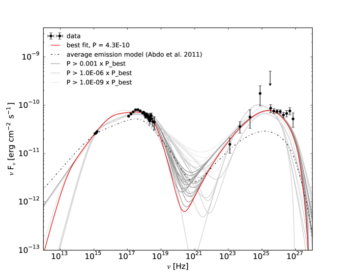
Figure 10: SED grid-scan modelling results for the flaring episode around MJD 54973 in the scope of a one-zone SSC scenario. Shown are the model curve (red solid line) with the highest probability of agreement with the data as well as model curves within different probability bands. For comparison, also the SSC one-zone model found to describe the average state (Abdo et al., 2011a) is given (black dash-dotted line). Data points have been corrected for EBL absorption according to the model by Franceschini et al. (2008).

The SED of Mrk 501 built from spectra around the time of the second flux increase seen by MAGIC on May 22 (MJD 54973) is shown in the bottom panel of Fig. 9 (see Sect. 3.1.2 and 3.1.1 for details on the individual observation times). The data related to the second flare were not taken strictly simultaneously. However, here the resulting caveat is not as strong as for the first flare. On one hand, the observed variability occurs on timescales of days, rather than tens of minutes, and the RXTE/PCA measurements were performed within a day from the VHE observations. While this is not true for the Swift/XRT measurements, the overall flux changes are relatively small, and the derived Swift/XRT spectrum is in very good agreement with the one derived from RXTE/PCA, as can be seen in the bottom panel of Fig. 9.

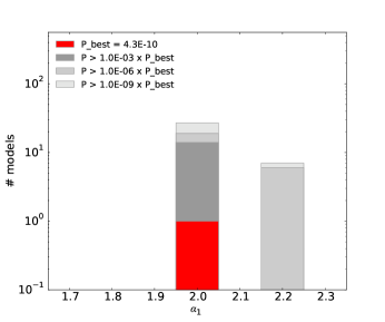
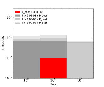
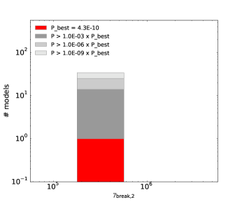
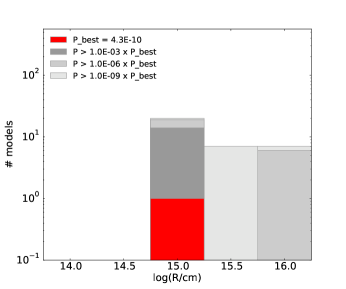
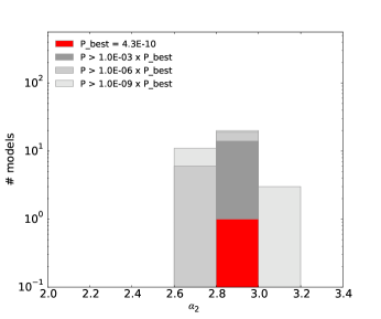
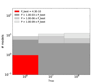
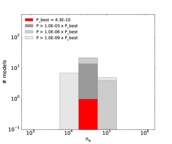
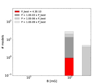
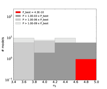
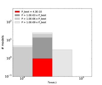
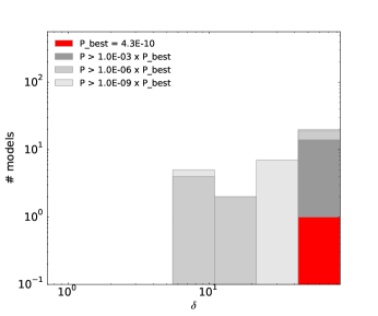
Figure 11: Number of SSC model curves with a fit probability above the given limits vs. each probed value of each model parameter. Given are the results for the coarse parameter grid within a one-zone scenario for MJD 54973. The X-axis of each plot spans over the probed range for each parameter. The figure shows the model with the highest probability of agreement to the data (red) and all models within several probability bands (different grey shades, see legend).

The results obtained for the one-zone scenario following the grid-scan from Tab. 5 gave a best probability of agreement with the data points of $P_{\text{best}}\approx 4\times 10^{-10}$ ($\chi^{2}/d.o.f.\approx 123/41$). We found that there are 14 additional SSC model curves with a model-to-data probability larger than 0.1% of the best-matching model (i.e. $P>10^{-3}\times P_{\text{best}}$), which we set as a generous probability threshold to consider the model-to-data agreement comparable. Given that $P_{\text{best}}\approx 4\times 10^{-10}$, even those models with comparatively best agreement $P>10^{-3}\times P_{\text{best}}$ do not adequately describe the measured broadband SED. Yet this relatively bad model-to-data agreement is not worse than some of the agreements between (simple) models and SED data shown in some studies (e.g. Abdo et al., 2010b; Giommi et al., 2012; Domínguez et al., 2013; Ahnen et al., 2016). This occurs because, in most studies involving broadband SEDs, the models are adjusted “by eye” to the data without any rigorous mathematical procedure that quantifies the model-to-data agreement. Differences on the order of 20%-30% in a log-log plot spanning many orders of magnitude do not “appear to be problematic”, despite these differences could be (statistically) significant due to the small errors from some of the data points (e.g. optical/UV and X-ray). If the differences between the data and model are not substantial (regardless of the statistical agreement), the models are considred to approximately describe the data and used to extract some physical properties of the source and its environment.

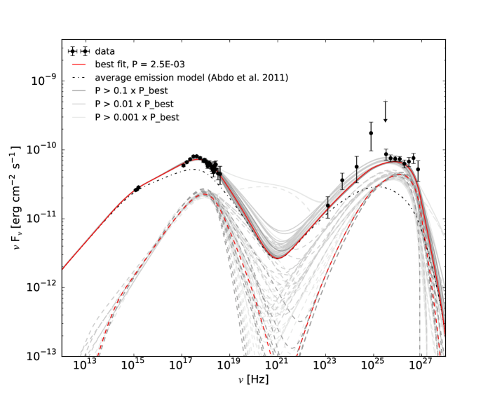
Figure 12: SED grid-scan modelling results for the flaring episode around MJD 54973 in the scope of a two-zone SSC scenario. The total emission (solid lines) is assumed to stem from a first quiescent region (black dot-dashed lines) responsible for the average state (Abdo et al., 2011a) plus a second emission region (dashed lines). The model with the highest probability of agreement with the data is highlighted in red. Model curves underlaid in grey show the bands spanned by models with a fit probability better than $0.1\times P_{\text{best}}$, $0.01\times P_{\text{best}}$ and $0.001\times P_{\text{best}}$, respectively. Data points have been corrected for EBL absorption according to the model by Franceschini et al. (2008).

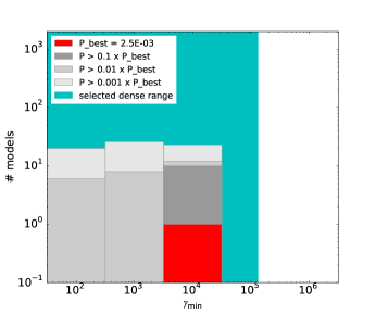
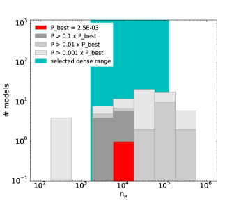
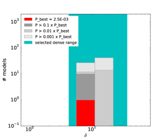
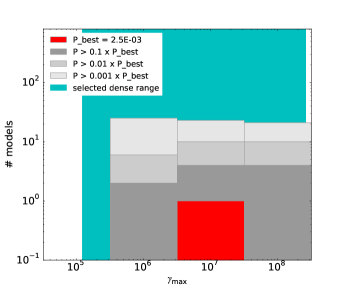
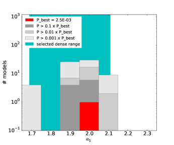
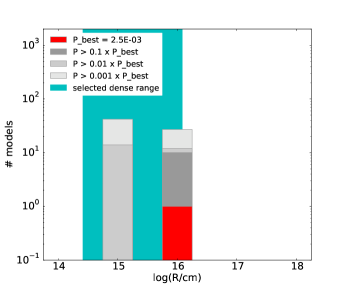
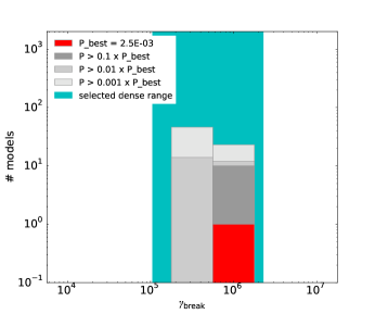
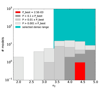
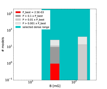
Figure 13: Number of SSC model curves which fulfill the given limits for the fit probability vs. each probed value of each model parameter. Shown are results for the coarse parameter grid-scan within a two-zone scenario for MJD 54973. The X-axis of each plot spans over the probed range for each parameter. Given are the model with the highest probability of agreement with the data and all models within the given probability bands (see legend). The parameter ranges chosen for the dense scan are also shown in each plot.

Figure 10 depicts the best SSC model curves from the one-zone scenario, with the model featuring the best agreement to the data shown with a red curve, and the other 14 SSC models with comparable (down to 0.1%) model-to-data agreement shown with dark-grey curves. Given the very low number of SSC model curves in this group, we decided to depict additionally those SSC models with model-to-data probability of agreement larger than $10^{-6}\times P_{\text{best}}$ and $10^{-9}\times P_{\text{best}}$ with lighter grey shades (see legend), which increased the number of SSC model curves depicted to 34. The thresholds used of $10^{-6}\times P_{\text{best}}$ and $10^{-9}\times P_{\text{best}}$ are somewhat arbitrary, and could be changed without any major qualitative impact in the reported results. The inclusion of these additional 20 models in the figure helps illustrate the behaviour of the SSC model curves that start being worse than the best-matching model. To guide the eye, the SSC model describing the average state is also shown (from Abdo et al., 2011a, dash-dotted black line). One can see that the most significant deviations of the model curves from the data points stem from the Swift region. Therefore, while the hard X-ray and $\gamma$-ray bands can be satisfactorily modeled with a one-zone SSC scenario, this model realization fails at reconstructing both the soft X-ray data points and the UV emission at the same time. Figure 11 displays how many model curves produced for each point on the parameter grid yield a model-to-data agreement probability $P$ better than $10^{-3}\times P_{\text{best}}$, which are the models that are considered to be comparable. This is shown for each of the parameters separately. One can see that some parameters are more constrained than others: e.g. $\gamma_{\text{break},1}$, $\gamma_{\text{break},2}$ and $\alpha_{2}$ show a narrower distribution than for instance $\gamma_{\text{max}}$ or $\alpha_{3}$, which lead to equally good models over essentially the entire range of values probed. Additionally, as done for Fig. 10, with lighter grey shades we also report the parameter values for $P>10^{-6}\times P_{\text{best}}$ and $P>10^{-9}\times P_{\text{best}}$. One can see that the SSC models that are not comparable to the best-matching model (i.e. those with $P<10^{-3}\times P_{\text{best}}$), have a similar distribution for those parameters that are not constrained, like $\gamma_{\text{max}}$ or $\alpha_{3}$. On the other hand, on the parameters that can be constrained, like $\gamma_{\text{break},1}$, and $\alpha_{2}$, these additional models extend the range of parameter values with respect to the distributions for the models with $P>10^{-3}\times P_{\text{best}}$. The parameter $\gamma_{\text{break},2}$ seems to be quite well constrained, and even the models with $P<10^{-3}\times P_{\text{best}}$ converge to the same value of 3.2$\times 10^{5}$. The implications of these distributions on the possibility to constrain the different model parameters will be further discussed in Sect. 5.

We also evaluated the model-to-data agreement for the one-zone scenario that uses the more simple grid-scan defined by Table 6, which is related to a grid of 9 parameters (instead of 11), but with a somewhat extended regions for some of these parameters. We found that this grid-scan did not provide any additional SSC model with $P>10^{-3}\times P_{\text{best}}$, and only five additional SSC models with $P>10^{-9}\times P_{\text{best}}$. Hence this grid-scan did not bring any practical improvement with respect to that from Table 5, that led to 14 SSC models with $P>10^{-3}\times P_{\text{best}}$, and 34 SSC models with $P>10^{-9}\times P_{\text{best}}$.

When using the above-mentioned two-zone SSC scenario, with the quiescent emission characterized by the model parameters from the average SED reported in Table 4, and the spatially independent region responsible for the flaring activity modeled based on the coarse grid parameter values reported in Table 6, we find a substantial improvement, with respect to the one-zone models, in describing the measured broadband SED (including the UV emission), with a best model-to-data probability of $P_{\text{best}}\approx 2.5\times 10^{-3}$ ($\chi^{2}/d.o.f.\approx 71/41$). The two-zone model provides a better description of the SED than the one zone model, but it still does not reproduces the data perfectly.

Fig. 12 displays the 69 SSC model curves with model-to-data agreement probability $P$ better than $10^{-3}\times P_{\text{best}}$, which is the generous probability threshold that we adopted to consider the probability of agreement comparable. Because of the relatively large number of SSC model curves (in comparison to those surviving the same selection criteria in the one-zone scenario), we decided to split those models into three groups according to their model-to-data probability $P$ being better than $10^{-1}\times P_{\text{best}}$, $10^{-2}\times P_{\text{best}}$ and $10^{-3}\times P_{\text{best}}$. Since $P_{\text{best}}\approx$0.25%, these models start providing an acceptable representation of the data, with the different bands reporting slightly different levels of success in the model-to-data agreement. The parameter values for those models are depicted in Fig. 13. As occurred for the one-zone scenario, some parameters are better constrained than others: e.g. $\gamma_{\text{break}}$ shows a narrow distribution, while $\gamma_{\text{min}}$ and $\gamma_{\text{max}}$ show a rather flat distribution. Despite the parameter $\gamma_{\text{min}}$ being probed up to $10^{6}$, the highest $\gamma_{\text{min}}$ values used in the SSC models that can adequately describe the broad-band SED go only up to $10^{4}$, which, for the highest B field values reported in Fig. 13 ($\sim$0.15 G), relate to a cooling time of $3.5\times 10^{6}$ seconds. This is one order of magnitude larger than the dynamical timescale set by the highest R values reported in Fig. 13 ($10^{16}$cm), hence ensuring the existence of a low-energy cutoff. See Sect. 5 for further discussions of this topic.

In order to refine the adjustment of the different model parameters even further, a second iteration of the grid-scan modelling, referred to as a dense grid-scan, is performed. The dense grid-scan focuses on the parameter ranges that provide the best model-to-data agreement in the coarse grid-scan, which are depicted in Fig. 13. Following this strategy, the chosen parameter ranges can be narrowed in favour of a smaller step size in the individual parameters, while keeping the computing time at a reasonable amount. The new dense grid ranges and number of steps for each of the parameters are given in Table 7.

The model with the highest probability of model-to-data agreement in the dense grid-scan yields $P_{\text{best}}\approx 6.6\times 10^{-2}$ ($\chi^{2}/d.o.f.\approx 55.4/41$), which implies an order of magnitude improvement with respect to the best-matching model obtained with the coarse grid-scan. If this model curve had been obtained through a regular mathematical fit, and conservatively considering that the nine dimensions of the grid relate to nine independent and free parameters in the fitting procedure, we would have obtained a p-value $\approx 6.3\times 10^{-3}$ ($\chi^{2}/d.o.f.\approx 55.4/32$). The dense grid-scan focussed on relatively good regions of the parameter space, which yielded a large number of SSC curves with a good model-to-data agreement despite the fact that the parameter values of this dense grid-scan still vary largely (implying very different physical conditions in the source). Because of the large number of model curves, we can be more demanding with the probability threshold for considering the probability of agreement comparable to that of the best-matching model: a probability threshold of $0.1\times P_{\text{best}}$ still keeps 1684 SSC models, which is a large increase in statistics, in comparison to the results obtained with the coarse scan. Given that $P_{\text{best}}\approx$6.6%, all the models above this probability threshold provide a decent representation of the data. We split these models into three groups according to their model-to-data agreement being $P>0.9\times P_{\text{best}}$, $P>0.5\times P_{\text{best}}$, and $P>0.1\times P_{\text{best}}$, hence reporting somewhat different levels of success in describing the measured broadband SED.

Also here we investigate the spread - or degeneracy - of the different models within the dense grid space of model parameters. Fig. 14 shows again the distribution of the best model (red) and the models with $P>0.9\times P_{\text{best}}$, $P>0.5\times P_{\text{best}}$ and $P>0.1\times P_{\text{best}}$, respectively, over the entire dense grid parameter space. In comparison to Fig. 13, one can notice an apparent larger degree of degeneracy, with distributions with entries in most of the probed parameter ranges depicted in the figure. The larger spread in the parameter values shown in Fig. 14 is caused by the selected parameter range, which is narrower and intentionally only covers regions with an already reasonable agreement between model and data, as derived from the coarse grid scan. Despite the large spread, one can see that there are regions with slightly better model-to-data agreement, like the region around $\gamma_{\text{break}}\sim 5\times 10^{5}$, or the region around $\alpha_{1}\sim 1.9$. The results will be further discussed in Sect. 5.

Table 7: Grid parameter space probed for two-zone models within the dense grid-scan applied to the flare around MJD 54973. The number of SSC models required to realize this grid-scan amounts to 212 million. See text for further details.

dense grid
two-zone	$\gamma_{\text{min}}$	$\gamma_{\text{max}}$	$\gamma_{\text{break}}$	$\alpha_{1}$	$\alpha_{2}$	ne	$\frac{\mathrm{B}}{\mathrm{mG}}$	$\log(\frac{R}{cm})$	$\delta$
min	$2.1\times 10^{1}$	$3.2\times 10^{5}$	$1.2\times 10^{5}$	1.7	3.5	$2\times 10^{3}$	20	14.5	5
max	$5\times 10^{4}$	$1\times 10^{8}$	$2\times 10^{6}$	2.1	5.0	$1\times 10^{5}$	200	16.0	30
$\#$ of steps	5	4	12	21	7	10	10	10	6
spacing	log	log	log	lin	lin	log	log	lin	lin

The SED models which are picked as a result of the dense grid-scan for two-zone SSC models are presented in Fig. 15. The figure highlights three SSC model curves: the model which gave the best agreement with the SED data points, a model featuring a prominent high-energy component in the EED, and a model that features a low Doppler factor of $\delta=5$. The parameter values for these three specific SSC model curves are given in Table 8, showing once more that three very distinct sets of SSC model parameters can provide comparable agreement with the experimental data.

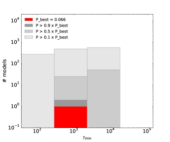
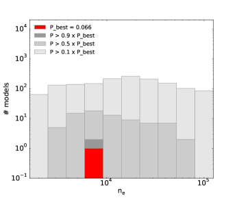
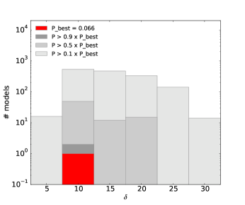
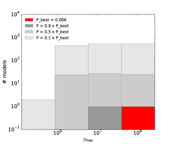
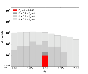
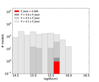
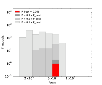
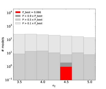
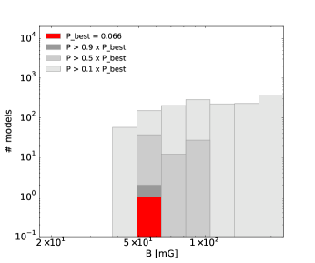
Figure 14: Distributions of the investigated models in the individual model parameters for the dense parameter grid and a two-zone scenario for MJD 54973. The X-axis of each plot spans over the probed range for each parameter. Shown are the model with the highest probability of agreement with the data and all models which populate the given probability bands (see legend).

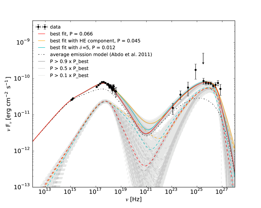
Figure 15: Modelling of the SED of Mrk 501 compiled from measurements collected during the high state observed around MJD 54973. Two-zone SSC models have been inspected following the grid-scan strategy. The total emission (solid lines) is assumed to stem from a first quiescent region (black dot-dashed lines) responsible for the average state (Abdo et al., 2011a) plus a second emission region (dashed lines). Highlighted are the model with the highest probability of agreement with the data (red), a model featuring a prominent high-energy component in the EED (orange), and a model with low Doppler factor (cyan, $\delta=5$). Model curves underlaid in grey show the bands spanned by models with a fit probability better than $0.9\times P_{\text{best}}$, $0.5\times P_{\text{best}}$ and $0.1\times P_{\text{best}}$, respectively. The data points have been corrected for EBL absorption according to the model by Franceschini et al. (2008).

Table 8: Results of the dense grid-scan SED modelling of the flaring episode around MJD 54973 in the scope of a two-zone SSC scenario. Quoted here are the three models highlighted in Fig. 15: the model with the best agreement to the data, a model with a prominent high-energy electron component, and a model with a remarkably low Doppler factor ($\delta=5$). Besides the model parameters, the reduced $\chi^{2}$ values, the fit probability compared to the best achieved fit probability, the departure from equipartition and the implied minimum variability timescale are also reported.

selected	$\gamma_{\text{min}}$	$\gamma_{\text{max}}$	$\gamma_{\text{break}}$	$\alpha_{1}$	$\alpha_{2}$	ne	$\frac{\mathrm{B}}{\mathrm{mG}}$	$\log(\frac{R}{cm})$	$\delta$	$\frac{\chi^{2}}{\mathrm{d.o.f.}}$	$\frac{\mathrm{P}}{\mathrm{P}_{\mathrm{best}}}$	$\frac{u_{e}}{u_{B}}$	$\frac{t_{\text{var}_{\text{min}}}}{\text{hour}}$
models
best $\chi^{2}$	$1\cdot 10^{3}$	$1.0\cdot 10^{8}$	$5.6\cdot 10^{5}$	1.90	4.5	$7.4\cdot 10^{3}$	56	15.7	10	55.4/41	1.00	933	4
HE comp	$1.0\cdot 10^{3}$	$1.5\cdot 10^{7}$	$4.3\cdot 10^{5}$	1.86	3.5	$4.8\cdot 10^{3}$	56	15.7	10	57.5/41	0.68	919	4
Low $\delta$	$1.5\cdot 10^{2}$	$1.5\cdot 10^{7}$	$5.6\cdot 10^{5}$	1.82	3.5	$2.0\cdot 10^{3}$	72	16.0	5	64.2/41	0.18	424	19

5 Discussion

5.1 Variability and correlations

For Mrk 501, an increase of the fractional variability with energy has been reported in the past within the X-ray and VHE band (Gliozzi et al., 2006; Albert et al., 2007a; Aliu et al., 2016). In the work presented here, we extend this trend throughout all wave-bands from radio to VHE $\gamma$-rays, showing that the source is relatively steady at radio/optical frequencies, but variable ($F_{\text{var}}\geq 0.2$) and very variable ($F_{\text{var}}\geq 0.4$) in the X-ray and VHE $\gamma$-ray bands, respectively, with a clear increase in the fractional variability with energy (observed in all the bands where we can measure). A similar variability pattern was reported in Aleksić et al. (2015b) and, during the preparation of this study, also in Ansoldi et al. (2016), in relation to the extensive campaigns on Mrk 501 performed in 2008 and 2012, respectively. This suggests that this variability vs. energy behaviour is an intrinsic characteristic in Mrk 501. On the other hand, Furniss et al. (2015) recently reported a different fractional variability vs. energy pattern based on observations taken in 2013, where the observed variability at X-rays is similar to that at VHE.

The multiband variability pattern that has been observed in Mrk 501 is quite different from that observed in Mrk 421 during the multi-instrument campaigns from 2009, 2010 and 2013, as reported in Aleksić et al. (2015a), Aleksić et al. (2015c) and Baloković et al. (2016). In those works a double-bump structure in the fractional variability plot was found (instead of a continuous increase with energy) which relates to the two bumps in the broadband SED, and where the highest variability occurs at X-rays and VHE, at comparable levels.

A clear correlation of the X-ray and VHE $\gamma$-ray emission was observed during the large and long $\gamma$-ray activity from 1997, as reported in e.g. Pian et al. (1998); Gliozzi et al. (2006), but this correlation was only marginally detected during the $\gamma$-ray flare observed in 2005 (Albert et al., 2007a). The low significance in the X-ray-to-VHE correlation during the flares in 2005 was ascribed to the lack of sensitive X-ray measurements during this observing campaign; only RXTE/ASM data, which has limited sensitivity to detect Mrk 501, was available for this study. A positive correlation between X-ray and VHE $\gamma$-rays was reported, for the first time, also during very low X-ray and VHE activity, but only at 99% confidence level (Aleksić et al., 2015b). The marginally significant correlation observed during this low activity, using data from the multi-instrument campaign in 2008, was ascribed to the very low variability during that campaign, where the measured $F_{var}$ values were about 0.1 for X-rays and 0.2 for VHE. As reported above, during the multi-instrument campaign in 2009, Mrk 501 was mostly in its low/typical state, but we also measured two flaring activities in May 2009. The measured $F_{var}$ is about 0.3 for X-rays and 0.8 for VHE, while if we exclude the two flaring episodes, we obtain $F_{var}$ values of about 0.2 for X-rays and 0.5 for VHE. However, despite the larger variability observed in 2009 (with respect to 2008), we did not observe any significant correlation between the X-ray and the VHE emission (including and excluding the flaring episodes). This may appear to be a controversial result, but we would like to stress that a very significant correlation with past data was only observed during the very large and long flare in 1997. Recently, Furniss et al. (2015) reported a significant X-ray-to-VHE correlation, using data from the multi-instrument campaign in 2013. This correlation is dominated by the large X-ray and VHE activity observed during four consecutive days in July 2013: although it still remains at 2 $\sigma$ (for the 0.3-3 keV energy band) and 5 $\sigma$ (for the 3-7 keV band) when removing the flaring activity. In conclusion, some multi-instrument campaigns on Mrk 501 do not show a clear X-ray to VHE correlation when the source is not flaring strongly or persistently high. However, for the other archetypical TeV blazar, Mrk 421, the X-ray-to-VHE correlation is significantly detected during both low- (e.g. Aleksić et al., 2015a; Baloković et al., 2016) and high-activity states (e.g. Fossati et al., 2008; Acciari et al., 2011; Aleksić et al., 2015c).

The X-ray-to-VHE correlation and the fractional variability vs. energy pattern observed in Mrk 421 suggests that the X-ray and VHE emissions are produced by the same electrons, within the framework of SSC scenarios, and that the highest variability is produced by the highest-energy and most-variable electrons, which dominate the emission at the keV and the TeV bands, respectively. Instead, in Mrk 501 we observe a continuous increase in the variability with energy and absence of persistent correlation between the keV and TeV emissions. This suggests that the highest-energy electrons, in the framework of SSC scenarios, are not responsible for the keV emission, while they are responsible (at least partially) for the TeV emission. Alternatively, there could be an additional (and very variable) component contributing to the $\gamma$-ray emission, in addition to that coming from the SSC scenario, like inverse-Compton of the high-energy electrons off some external low-energy photon fields (Dermer et al., 1992; Sikora et al., 1994; Finke, 2016).

5.2 The VHE flaring state SEDs

The first flaring event (MJD 54952) is characterized by a fast and large outburst in the VHE band, which was apparently not accompanied by a substantial increase of the X-ray flux, and hence appeared to be like an “orphan flare” (see e.g. Krawczynski et al., 2004). In fact, based on these observations, this event was indeed tentatively categorized as an “orphan flare” event (Pichel & Paneque, 2011; Neronov et al., 2012), which would substantially challenge the currently favoured SSC emission models (for HBLs). However, a detailed look at the SED of the flaring episode reveals a hardening of the X-ray spectrum measured by Swift/XRT (see Sect. 3), which more likely corresponds to a shift of the synchrotron bump towards higher energies. During the outstanding activity in 1997, the synchrotron peak was shifted to beyond 100 keV, as accurately measured by BeppoSax (Pian et al., 1998). Such a large increase in the location of the synchrotron peak position could have occurred in the MJD 54952 flare discussed here. Additionally, the peak of the high-energy $\gamma$-ray bump at the time of this flare also appears to shift towards higher energies, as occurred in 1997. This suggests a more general appearance of such phenomena, and that, even though the measured keV and TeV flux are not correlated during this flaring activity, the overall broad band X-ray and VHE emission may still be correlated, which could have been measured if X-ray observations at several 10s of keV had been available during this flaring episode. Such a shift of the entire SED has been interpreted as a shift in the energy distribution of the radiating electron population (e.g. Pian et al., 1998; Albert et al., 2007a). In this context, the small change in the inverse Compton peak position compared to that of the synchrotron peak location could be ascribed to Klein-Nishina effects. High-energy electrons can efficiently produce high-energy synchrotron photons; however their effectiveness to upscatter photons reduces with respect to the lower-energy electrons because the Klein-Nishina cross-section is smaller than the Thomson cross-section (Tavecchio et al., 1998; Acciari et al., 2011).

We tried to parameterize the broadband SED during this first flare (MJD 54952) using a wide range of SSC emission scenarios following the grid-scan strategy defined in Sect. 4.1, allowing for models with one or two (independent) emission zones and covering a wide range in the space of model parameters. We found that none of the tested models could satisfactorily reproduce the changes observed in the spectral distribution. This broad-band SED may be explained with more sophisticated theoretical models, like the inhomogeneous time-dependent models reported in Ghisellini et al. (2005); Graff et al. (2008); Chen et al. (2011, 2015, 2016), which provide a more elaborate physical scenario, at the expense of an increase in the number of degrees of freedom of the model. However, a caveat has to be taken into account when interpreting these results, which is the lack of strict simultaneity of the different data sets, in particular the Swift/XRT and the VHE $\gamma$-ray data. The individual exposure times are separated by seven hours, while we see flux changes by a factor of $\sim$4 on sub-hour timescales, as reported in Pichel & Paneque (2011) and Aliu et al. (2016). Therefore, it is somewhat uncertain whether the measurements of the synchrotron peak and the high-energy peak probe the same source state. In the recent study reported in Aliu et al. (2016), the broadband SED derived for the 3-day time interval MJD 54952–55 could be satisfactorily parameterized with a one-zone SSC scenario that differs from the one used here and in Abdo et al. (2011a) in various aspects, including the template used to describe the host galaxy contribution.

Compared to the first flaring event, the second flare ($\approx$ MJD 54973) occurs during VHE flux changes of factors of $\sim$2 on timescales of a few days, and hence the lack of strict simultaneity in the X-ray/VHE observations is a much smaller caveat than for the first flaring event. In this case, again following the grid-scan modeling approach, one-zone SSC models were found unable to describe the measured SED, reaching best probabilities of agreement $\sim 10^{-10}$). The two-zone SSC models were able to reproduce the experimental observations better, reaching best probabilities of agreement $\sim 10^{-3}$). Therefore, the two-zone scenario appears to be favoured compared to the one-zone scenario considered here. Building on the range of two-zone model parameters providing decent data-model agreement, a fine grid-scan was performed, yielding hundreds of two-zone SSC models with probabilities of agreement $\sim 10^{-2}$. The obtained set of two-zone SSC models providing the best agreement comprises several set-ups with quite different implications for the parameters defining the EED and the surrounding region of the second emission region (see Sect. 4.3).

Comparing the configurations obtained for the emission region responsible for the second flare with the parameter values describing the emission region assumed to create the quiescent emission, some general trends can be stated: while the parameters describing the EED and the Doppler factor are found to populate roughly the same ranges of values, the electron density n_e is increased by 1-2 orders of magnitude, the magnetic field is larger by $\approx 1$ order of magnitude and the size of the emission region $\mathrm{R}$ is found to be smaller by 1-2 orders of magnitude. The latter result is affected by the requirement of a minimum variability timescale of a day, in order to account for the variability seen in the data.

Besides the general observations made above, some interesting model configurations stand out from the set of adequate scenarios: models which feature a prominent high-energy component in the EED, and models with Doppler factors as low as $\delta=5$ can be used to adequately model the flaring SED. In the paragraphs below we discuss the benefits of these two families of models.

Synchrotron self-Compton models with a strong high-energy component are interesting not only to explain the SED collected during the presented campaign, but also in the context of other observations of Mrk 501. During the extreme flare seen in 1997, a strong increase in the regime of hard X-rays, around 100 keV, was observed (Bradbury et al., 1997). This increase can be interpreted as the emergence of a strong high-energy component adding to the overall SED, which only becomes visible sometimes during extreme flaring states. Moreover, Cherenkov telescope observations often give hints of an additional hard component in the EED during flaring times: in Albert et al. (2007a) a significant spectral hardening during flaring states was observed and reported for the first time, and in the course of several more observational campaigns this “harder when brighter” behaviour has been established as typical for Mrk 501. Ultimately, a tendency for this behaviour was also seen during the campaign presented in this paper. In this light, SSC models with such a high-energy contribution to the EED could be favoured, as they can also explain such mentioned observations. Naturally, with the data set at hand and the lack of hard X-ray observations above $\approx 20$ keV, they can neither be confirmed nor discarded.

The finding that models with $\delta=5$ can also adequately reconstruct the data is particularly interesting. Quite high values (above $\delta=10$, up to $\delta=50$ or more) are usually required to model the SEDs of blazars (Tavecchio et al., 1998; Krawczynski et al., 2001; Saugé & Henri, 2004). These high Doppler factors are in tension with regard to expectations from the small (typically less than $2c$) apparent velocities observed in the 43 GHz radio emission of various high-peaked BL Lac objects, and particularly with that measured for Mrk 501 (Edwards & Piner, 2002; Piner & Edwards, 2004; Piner et al., 2010). This has posed a common problem for TeV sources, which has been dubbed the “bulk Lorentz factor crisis” (Henri & Saugé, 2006), and requires the radio and TeV emission to be produced in regions with different bulk Lorentz factors. Debates on this problem (see for example Georganopoulos & Kazanas, 2003; Levinson, 2007; Stern & Poutanen, 2008) have led to a series of sophisticated models, e.g. the ”spine-sheath” model from Ghisellini et al. (2005), in which the jet is structured transverse to its axis into a fast “spine” that produces the high-energy emission, and a slower “layer” which dominates the radio emission. The modeling results presented in this paper show that it is actually possible to model the SED of a flaring activity of Mrk 501 using a relatively small Doppler factor to describe the flaring emission, hence alleviating the tension with the radio interferometric observations. Naturally, such low Doppler factors cannot be used for broad-band SEDs related to periods with fast (sub-hour) variability, such as the one from MJD 54952; but they can be be used for broad-band SEDs related to flaring activities with day timescales, such as the one from MJD 54973, which are more commonly observed in high-peaked BL Lac objects.

In addition to individual models which give a good reproduction of the data, the degree of degeneracy of well-fitting models in the individual parameters has also been studied, revealing a wide range of equally good models in the SSC parameter space, and showing that some model parameters can be constrained much better than others. While this can be seen already for the one-zone SSC models, where e.g. $\gamma_{break,1}$ and $\gamma_{break,2}$ show a narrower distribution than for instance $\gamma_{max}$ or $\alpha_{3}$, it is particularly interesting to study this for the more applicable two-zone scenario, which is the one that describes suitably the data. We find that for both the coarse and the dense grid-scan, the distribution of parameter values giving a good agreement with the data is quite well constrained for some parameters, such as the Lorentz factor at the break energy of the electrons $\gamma_{\text{break}}$, while other parameters show a rather broad distribution, like $\gamma_{\text{max}}$ or the index of the EED after the break $\alpha_{2}$, which points to a real degeneracy in these parameters. To some extent this degeneracy can be explained by the unequal sampling of the SED: the density and accuracy of measurements at or around the positions of the synchrotron and the IC peak is rather dense, which leads to a good definition of the spectral break in the EED. However, moving from the peak positions up to higher energies, the uncertainties of the measurements increase (especially for the synchrotron peak) and parameters such as the spectral index after the break $\alpha_{2}$ or the Lorentz factor where the EED is cut off $\gamma_{\text{max}}$ cannot be constrained equally well.

This result has several implications for the modeling of SEDs in general. On one hand, it shows that an actual fitting procedure, which moves along the direction of the steepest gradient in the parameter space towards a minimum in e.g. the $\chi^{2}$ of the model-to-data agreement, does not necessarily reveal the entire picture of possible descriptions of the data in the context of the applied model. Usually one “best” solution is quoted as the result, while most of the time a wide range of models explain the data equally well. We also see that, in order to be able to put stronger constraints on the parameters defining SED models, we need data sets which are characterized by a better coverage in energy and by smaller uncertainties in flux. We see in Fig. 15 that especially the hard X-ray regime, but also the HE and VHE $\gamma$-ray regime, are allowing for a wide range of possible model curves.

Unfortunately, the here-presented exercise indicates that the SED modeling results which are performed for less constrained data sets, e.g. for “weak sources” which are sampled with much less coverage in energy and with less statistics, should be taken with caution because are likely to have substantial degeneracies in the model parameters. Such modeling exercises can demonstrate that a particular scenario (e.g. one-zone or two-zone SSC) is capable of reproducing the measured data, but they certainly cannot claim the exclusiveness or even the prominence of the particular set of parameter values that has been chosen or found to be “best”.

5.3 Change in optical polarization during VHE $\gamma$-ray flare

The first VHE flare (MJD 54952) was found to coincide with an observed change in the optical polarization. While simulations of turbulent processes in blazar jets show that a rotation of this dimension can be ascribed to random behaviour (Marscher, 2014), the coinciding occurrence of the change in rotation and a flare of the VHE $\gamma$-ray flux suggests a common origin of these events. Such combined events have already been seen in low-frequency peaked BL Lac type sources (LBL) and flat spectrum radio quasars (FSRQ), but it has been observed for the first time for an HBL in the course of the 2009 campaign, and already reported in Pichel & Paneque (2011); Aliu et al. (2016).

These observations show similarities to double or multiple flaring events seen in the LBL BL Lacertae in 2005 and in the FSRQ PKS 1510-089 in 2009, which were discussed by Marscher et al. (2008) and Marscher et al. (2010), respectively.

Exhibiting different peak frequencies for the synchrotron and the IC bump, the optical variability seen in BL Lac could be seen as corresponding to the X-ray variability in Mrk 501. While a strong flare in the VHE band has been observed during the first flare of Mrk 501, BL Lac gives hints for activity in that band during the first optical outburst (Albert et al., 2007b). A coincidence of a flaring event and a change in the optical polarization is seen in all three data sets. The observed degree in optical polarization in Mrk 501 of $\approx 5\%$ appears to be small in comparison to that in BL Lacertae (up to $18\%$). Still, the optical flux in Mrk 501 is strongly dominated by the host galaxy, so that the jet contribution amounts to only $\sim$1/3. Therefore, the measured degree of polarized light in Mrk 501 corresponds to a fraction of $\approx 15-20\%$ of polarized emission from the jet, which is comparable to BL Lacertae. The second episode of high activity in both Mrk 501 and BL Lac was characterized by an increased flux at the synchrotron bump over a longer time span.

In the case of BL Lac, Marscher et al. (2008) suggested that the “first” flare and the change in polarization may have occurred when a blob of highly energetic particles travels along the last spiral arm of a helical path within the acceleration and collimation zone of the jet, and finally leaves this zone to enter a more turbulent region. The “second” flare seen in BL Lac has been identified with the passage of the feature through the shocked region of the radio core. The observed behaviour of Mrk 501 suggests that the discussed scenario could be applicable here. Despite the lack of simultaneous interferometric radio observations during both flares, an enhancement of the activity in the VLBA 43 GHz core emission in May 2009 (with respect to the previous months) was observed, supporting the interpretation of the blob traversing a standing shock region during the second flaring episode.

The polarization data collected during this campaign could also hint at a different physical scenario. After the VHE flare on MJD 54952, not only did the EVPA rotation stop, but it also started rotating in the reverse direction during the following 2 days, and the polarization degree did not drop to the ”typical low-state values” of about 1–2%, but only decreased from 5.4% to 4.5% (see the two bottom panels from Fig. 1). The characteristics of the polarization data after the VHE flare may be better explained as resulting from light-travel-time effects in a straight shock-in-jet model with helical magnetic fields, as proposed by Zhang et al. (2014, 2015). This shock-in-jet model, which uses a full three-dimensional radiation transfer code and takes into account all light–travel–time and other geometric effects (for some assumed geometries), may be more successful in explaining the broad-band SED (and variability patters) observed during the VHE flare from MJD 54952, which could not be explained with the ”relatively simple” one-zone and two-zone SSC scenarios described in Sect 4. However, the lack of strictly simultaneous X-ray/VHE data during the MJD 54952 VHE flare, and the relatively scarce polarization observations after the VHE flare would be an important limitation in the full application of this theoretical scenario to the here-presented multi-instrument data set.

6 Summary and concluding remarks

We presented a detailed study of the MWL variability of the HBL Mrk 501, based on a multi-instrument campaign that was conducted over 4.5 months in 2009, with the participation of MAGIC, VERITAS, the Whipple 10 m, Fermi-LAT, RXTE, Swift, GASP-WEBT, and several optical and radio telescopes. Mrk 501 shows an increase in the fractional variability with energy, from a steady flux at radio and optical frequencies to fast and prominent flux changes in the VHE $\gamma$-ray band. Overall, no significant correlation was found between any of the measured energy bands, particularly no correlation was seen between X-rays and VHE $\gamma$-rays, despite the relatively large variability measured in these two energy bands. This suggests that the highest-energy (and most variable) electrons that are responsible for the VHE $\gamma$-rays measured by MAGIC, VERITAS and Whipple 10 m, do not have a dominant contribution to the $\sim$1 keV emission measured by Swift/XRT. These high-energy electrons may have a dominant contribution to the hard X-ray emission above 10–50 keV, where the instrumentation used in this campaign did not provide sensitive data. Alternatively, there could be a component contributing to the VHE $\gamma$-ray emission in addition the component coming from the SSC scenario (e.g. external Compton), which is highly variable and further increases the variability of Mrk 501 at VHE $\gamma$-rays with respect to that expected from the pure SSC scenario.

This paper discusses two prominent flaring events at VHE $\gamma$-rays with different characteristics that were seen during the campaign. The first flare is dominated by a fast outburst in the VHE range, which does not appear to be accompanied by a large flux increase in the X-ray band, but shows a hardening in the X-ray spectrum that can be associated with a shift of the synchrotron bump to higher energies. On the other hand, the second flare is characterised by a flux increase in both the VHE and the X-ray band. For the parameterisation of the broadband SEDs from these two VHE $\gamma$-ray flares, we applied a novel variation of the grid-scan approach in the space of model parameters. For the two theoretical scenarios investigated, the one-zone and two-zone SSC models, we probed multi-dimensional grids with the various model parameters, evaluating the model-to-data agreement for tens of millions of SSC models. This strategy allowed us to identify disjointed regions of equally good model configurations, and provided a quantification of the degeneracy in the model parameters that describe the measured broadband SEDs. The presented methodology provides a less biased interpretation than the commonly used “single-curve model adjustment procedure” typically reported in the literature.

A lack of strict simultaneity in the X-ray/VHE observations of the first flare, which is characterized by large VHE flux changes in sub-hour timescales, does not permit us to draw final conclusions on the underlying mechanism; but the SED modeling with the grid-scan suggests that a simple one-zone or two-independent-zone SSC model is not sufficient to explain the measured broadband emission. The broadband SED derived for the second flare also lacks strictly simultaneous observations, but the flux changes here are smaller and on longer timescales, and hence substantially less problematic than for the first flare. The overall SED from the second flare cannot be properly described by a one-zone SSC model (with an EED with two spectral breaks), while it can be reproduced satisfactorily within a two-independent-zone SSC scenario. In the two-zone models applied here, one zone is responsible for the quiescent emission from the averaged 4.5-month observing period, while the other one, which is spatially separated from the first, dominates the flaring emission occurring at X-rays and VHE $\gamma$-rays. The grid-scan shows that there is a large number of SSC model realizations that describe the broadband SED data equally well, and hence that there is substantial degeneracy in the model parameters despite the relatively well-measured broadband SEDs. For instance, regarding the features of the EED, the position of the break(s) appear to be well constrained, while the highest Lorentz factor and the high-energy spectral index vary more strongly within the best-fitting model realizations. While the few models with the best relative agreement to the data feature Doppler factors $\delta$ in the range 10–20, the data can also be reproduced using substantially lower Doppler factors of $\delta=5$ while still reaching fit probabilities higher than $10\%\,P_{\text{best}}$. This shows that it is possible to reproduce the observed SED from Mrk 501 assuming boost factors well below the usually required values of $\delta\approx 10-50$, which may loosen a bit the tension posed between large values of $\delta$ required for modeling and low values imposed from radio velocity measurements, which has been dubbed the “bulk Lorentz factor crisis”.

A change in the rotation of the EVPA was measured in temporal coincidence with the first VHE flare, at MJD 54952, as reported in Pichel & Paneque (2011); Aliu et al. (2016). Here we also show that during the first VHE flare, the degree of polarization increased by a factor of $\sim$3 with respect to the polarisation measured before and after this flaring activity. This is the first time that such behaviour is observed in Mrk 501, or in any other HBL object, and suggests a common origin of the VHE flare and the optical polarized emission. With the coincidence seen of a VHE flare and changes in the trend of the optical polarization, this two-flare event resembles prior events observed in the LBL BL Lacertae and the FSRQ PKS 1510-089, which were discussed in Marscher et al. (2008) and Marscher et al. (2010), respectively. The common features suggest a similar interpretation of the flaring event of Mrk 501 as an emission region which is traveling upstream of the radio core along a spiral path in a helical magnetic field, entering a region of turbulent plasma and crossing the standing shock region of the radio core. After the VHE flare at MJD 54952, the polarization degree decreased from 5.4% to only 4.5% (instead of the typical low-state value of 1–2%), and there is also a small EVPA rotation in the reverse direction during the following 2 days, which may be difficult to explain with the typical helical pattern motions mentioned above; they may be better explained as light-travel-time effects in a shock-in-jet model in a straight, axisymmetric jet embedded in a helical magnetic field, as reported in Zhang et al. (2014, 2015). Beyond the interpretation of the flaring event itself, the observational results obtained in the course of this MWL campaign reveal phenomena that have not been seen for any HBL before, but have already been studied for LBLs and FSRQs. This gives a strong indication of the intrinsic similarity of these blazar subclasses, despite showing different jet characteristics in general, such as apparent jet speed and the overall power output. Observations of rapid variability in the LBL BL Lacertae (Arlen et al., 2013) support this further, as such fast flux changes had only been seen in HBL observations.

Additional multi-instrument observations of Mrk 501 will be crucial to confirm and extend several of the observations presented here. First of all, the large degeneracy in the model parameter values providing an acceptable description of the broadband SED is largely dominated by the poor coverage at hard X-rays, as well as the somewhat limited resolution at VHE $\gamma$-rays. Since mid-2012, NuSTAR provides excellent sensitivity above 10 keV, which narrows down the large gap in the SED between soft X-rays and the Fermi-LAT regime for campaigns from 2012 onwards. In the coming years, observations with ASTROSAT will also be possible, hence facilitating a much more accurate characterization of the evolution of the synchrotron bump of Mrk 501, including the determination of hard components in the EED whose synchrotron emission may peak at 50 or 100 keV. Moreover, in the regime of VHE $\gamma$-rays, data sets of much higher quality are already being collected, yielding a better resolution and an extended energy coverage. This is achieved on the one hand by the operation of the MAGIC telescopes as a stereo system, which gave a remarkable improvement in the overall performance compared to the mono mode which was still operational during the campaign reported in this paper (Aleksić et al., 2012). On the other hand, both MAGIC and VERITAS underwent major upgrades in the years 2011 and 2012, which gave a further substantial push to the performance (Aleksić et al., 2016a, b; Zitzer et al., 2013). In the future, the Cherenkov Telescope Array (CTA) promises to deliver further, substantial improvement both in terms of the energy coverage and the resolution of the flux measurement (Actis et al., 2011). Additionally, the temporal coverage extending over many years will permit variability studies (including many flares) over large portions of the electromagnetic spectrum and with good sensitivity, which will permit one to evaluate whether the association of EVPA rotations and polarization degree changes with VHE $\gamma$-ray flares are rare or regular events, whether these events occur together with a second flaring activity with contemporaneous enhancement of the VLBA radio core emission, and whether the measured multiband variability and lack of 1 keV–1 TeV correlation is a typical characteristic in Mrk 501 that gets repeated over time.

References

- Abdo et al. (2009) Abdo, A. A., Ackermann, M., Ajello, M., et al. 2009, ApJ, 699, 817
- Abdo et al. (2010a) Abdo, A. A., Ackermann, M., Ajello, M., et al. 2010a, ApJ, 710, 1271
- Abdo et al. (2010b) Abdo, A. A., Ackermann, M., Agudo, I., et al. 2010b, ApJ, 716, 30
- Abdo et al. (2011a) Abdo, A. A., Ackermann, M., Ajello, M., et al. 2011a, ApJ, 727, 129
- Abdo et al. (2011b) Abdo, A. A., Ackermann, M., Ajello, M., et al. 2011b, ApJ, 736, 131
- Acciari et al. (2011) Acciari, V. A., Aliu, E., Arlen, T., et al. 2011, ApJ, 738, 25
- Acciari et al. (2011) Acciari, V. A., Arlen, T., Aune, T., et al. 2011, ApJ, 729, 2
- Acero et al. (2015) Acero, F., Ackermann, M., Ajello, M., et al. 2015, The Astrophysical Journal Supplement Series, 218, 23
- Acero et al. (2016) Acero, F., Ackermann, M., Ajello, M., et al. 2016, ApJS, 223, 26
- Actis et al. (2011) Actis, M., Agnetta, G., Aharonian, F., et al. 2011, Experimental Astronomy, 1
- Aharonian et al. (2001) Aharonian, F., Akhperjanian, A., Barrio, J., et al. 2001, ApJ, 546, 898
- Ahnen et al. (2016) Ahnen, M. L., Ansoldi, S., Antonelli, L. A., et al. 2016, MNRAS, 459, 3271
- Albert et al. (2007a) Albert, J., Aliu, E., Anderhub, H., et al. 2007a, ApJ, 669, 862
- Albert et al. (2007b) Albert, J., Aliu, E., Anderhub, H., et al. 2007b, ApJ, 666, L17
- Albert et al. (2008) Albert, J., Aliu, E., Anderhub, H., et al. 2008, ApJ, 674, 1037
- Aleksić et al. (2012) Aleksić, J., Alvarez, E. A., Antonelli, L. A., et al. 2012, Astroparticle Physics, 35, 435
- Aleksić et al. (2014) Aleksić, J., Ansoldi, S., Antonelli, L. A., et al. 2014, A&A, 572, A121
- Aleksić et al. (2015a) Aleksić, J., Ansoldi, S., Antonelli, L. A., et al. 2015a, A&A, 576, A126
- Aleksić et al. (2015b) Aleksić, J., Ansoldi, S., Antonelli, L. A., et al. 2015b, A&A, 573, A50
- Aleksić et al. (2015c) Aleksić, J., Ansoldi, S., Antonelli, L. A., et al. 2015c, A&A, 578, A22
- Aleksić et al. (2016a) Aleksić, J., Ansoldi, S., Antonelli, L. A., et al. 2016a, Astroparticle Physics, 72, 61
- Aleksić et al. (2016b) Aleksić, J., Ansoldi, S., Antonelli, L. A., et al. 2016b, Astroparticle Physics, 72, 76
- Aliu et al. (2016) Aliu, E., Archambault, S., Archer, A., et al. 2016, A&A, 594, A76
- Anderhub et al. (2009) Anderhub, H., Antonelli, L. A., Antoranz, P., et al. 2009, ApJ, 705, 1624
- Ansoldi et al. (2016) Ansoldi, S., Antonelli, L. A., Antoranz, P., et al. 2016, In preparation
- Arévalo et al. (2009) Arévalo, P., Uttley, P., Lira, P., et al. 2009, The Monthly Notices of the Royal Astronomical Society, 397, 2004
- Arlen et al. (2013) Arlen, T., Aune, T., Beilicke, M., et al. 2013, ApJ, 762, 92
- Baloković et al. (2016) Baloković, M., Paneque, D., Madejski, G., et al. 2016, ApJ, 819, 156
- Baring et al. (2016) Baring, M. G., Boettcher, M., Summerlin, E. J. 2016, MNRAS ArXiv e-prints (arXiv:1609.03899)
- Bradbury et al. (1997) Bradbury, S. M., Deckers, T., Petry, D., et al. 1997, Astronomy and Astrophysics, 320, L5
- Catanese et al. (1997) Catanese, M., Bradbury, S. M., Breslin, A. C., et al. 1997, ApJ, 487, L143
- Cerruti et al. (2013) Cerruti, M., Boisson, C., & Zech, A. 2013, Astronomy and Astrophysics, 558, A47
- Chen et al. (2011) Chen, X., Fossati, G., Liang, E. P., & Böttcher, M. 2011, MNRAS, 416, 2368
- Chen et al. (2015) Chen, X., Pohl, M., & Böttcher, M. 2015, MNRAS, 447, 530
- Chen et al. (2016) Chen, X., Pohl, M., Böttcher, M., & Gao, S. 2016, MNRAS, 458, 3260
- Dermer et al. (1992) Dermer, C. D., Schlickeiser, R., & Mastichiadis, A. 1992, A&A, 256, L27
- Djannati-Atai et al. (1999) Djannati-Atai , A., Piron, F., Barrau, A., et al. 1999, A&A, 350, 17
- Domínguez et al. (2013) Domínguez, A., Finke, J. D., Prada, F., et al. 2013, ApJ, 770, 77
- Domínguez et al. (2011) Domínguez, A., Primack, J. R., Rosario, D. J., et al. 2011, Monthly Notices of the Royal Astronomical Society, 410, 2556
- Edelson & Krolik (1988) Edelson, R. A. & Krolik, J. H. 1988, Astrophysical Journal, 333, 646
- Edwards & Piner (2002) Edwards, P. G. & Piner, B. G. 2002, ApJ, 579, L67
- Finke (2016) Finke, J. 2016, ArXiv e-prints (arXiv:1602.05965) [arXiv:1602.05965]
- Finke et al. (2010) Finke, J. D., Razzaque, S., & Dermer, C. D. 2010, ApJ, 712, 238
- Fomin et al. (1994) Fomin, V. P., Stepaniana, A. A., Lamb, R. C., et al. 1994, Astroparticle Physics, 2, 137
- Fossati et al. (2008) Fossati, G., Buckley, J. H., Bond, I. H., et al. 2008, ApJ, 677, 906
- Franceschini et al. (2008) Franceschini, A., Rodighiero, G., & Vaccari, M. 2008, Astronomy and Astrophysics, 487, 837
- Furniss et al. (2015) Furniss, A., Noda, K., Boggs, S., et al. 2015, ApJ, 812, 65
- Georganopoulos & Kazanas (2003) Georganopoulos, M. & Kazanas, D. 2003, ApJ, 594, L27
- Ghisellini et al. (2005) Ghisellini, G., Tavecchio, F., & Chiaberge, M. 2005, Astronomy and Astrophysics, 432, 401
- Giannios et al. (2009) Giannios, D., Uzdensky, D. A., & Begelman, M. C. 2009, MNRAS, 395, L29
- Giommi et al. (2012) Giommi, P., Polenta, G., Lähteenmäki, A., et al. 2012, A&A, 541, A160
- Giroletti et al. (2008) Giroletti, M., Giovannini, G., Cotton, W. D., et al. 2008, A&A, 488, 905
- Gliozzi et al. (2006) Gliozzi, M., Sambruna, R. M., Jung, I., et al. 2006, ApJ, 646, 61
- Graff et al. (2008) Graff, P. B., Georganopoulos, M., Perlman, E. S., & Kazanas, D. 2008, ApJ, 689, 68
- Henri & Saugé (2006) Henri, G. & Saugé, L. 2006, ApJ, 640, 185
- Horan et al. (2007) Horan, D., Atkins, R. W., Badran, H. M., et al. 2007, ApJ, 655, 396
- Kataoka et al. (1999) Kataoka, J., Mattox, J. R., Quinn, J., et al. 1999, Astroparticle Physics, 11, 149
- Katarzyński et al. (2006) Katarzyński, K., Ghisellini, G., Tavecchio, F., Gracia, J., & Maraschi, L. 2006, MNRAS, 368, L52
- Koyama et al. (2015a) Koyama, S., Kino, M., Doi, A., et al. 2015a, PASJ, 67, 67
- Koyama et al. (2015b) Koyama, S., Kino, M., Giroletti, M., et al. 2015, arXiv:1505.04433
- Krawczynski et al. (2004) Krawczynski, H., Hughes, S. B., Horan, D., et al. 2004, ApJ, 601, 151
- Krawczynski et al. (2001) Krawczynski, H., Sambruna, R., Kohnle, A., et al. 2001, ApJ, 559, 187
- Larionov et al. (2008) Larionov, V. M., Jorstad, S. G., Marscher, A. P., et al. 2008, A&A, 492, 389
- Lefa et al. (2011a) Lefa, E., Aharonian, F. A., & Rieger, F. M. 2011a, ApJ, 743, L19
- Lefa et al. (2011b) Lefa, E., Rieger, F. M., & Aharonian, F. 2011b, ApJ, 740, 64
- Levinson (2007) Levinson, A. 2007, ApJ, 671, L29
- Mankuzhiyil et al. (2012) Mankuzhiyil, N., Ansoldi, S., Persic, M., et al. 2012, ApJ, 753, 154
- Mankuzhiyil et al. (2011) Mankuzhiyil, N., Ansoldi, S., Persic, M., & Tavecchio, F. 2011, ApJ, 733, 14
- Marscher (2014) Marscher, A. P. 2014, ApJ, 780, 87
- Marscher et al. (2008) Marscher, A. P., Jorstad, S. G., D’Arcangelo, F. D., et al. 2008, Nature, 452, 966
- Marscher et al. (2010) Marscher, A. P., Jorstad, S. G., Larionov, V. M., et al. 2010, ApJ, 710, L126
- Massaro et al. (2004) Massaro, E., Perri, M., Giommi, P., Nesci, R., & Verrecchia, F. 2004, A&A, 422, 103
- Mattox et al. (1996) Mattox, J. R., Bertsch, D. L., Chiang, J., et al. 1996, ApJ, 461, 396
- Moretti et al. (2005) Moretti, A., Campana, S., Mineo, T., et al. 2005, UV, 5898, 360
- Neronov et al. (2012) Neronov, A., Semikoz, D., & Taylor, A. M. 2012, Astronomy and Astrophysics, 541, 31
- Nilsson et al. (2007) Nilsson, K., Pasanen, M., Takalo, L. O., et al. 2007, Astronomy and Astrophysics, 475, 199
- Padovani & Giommi (1995) Padovani, P. & Giommi, P. 1995, Astrophysical Journal, 444, 567
- Petry et al. (2000) Petry, D., Böttcher, M., Connaughton, V., et al. 2000, ApJ, 536, 742
- Pian et al. (1998) Pian, E., Vacanti, G., Tagliaferri, G., et al. 1998, ApJ, 492, L17
- Pichel & Paneque (2011) Pichel, A. & Paneque, D. 2011, Proceedings from the International Cosmic Ray Conference (arXiv:1110.2549) [1110.2549v1]
- Piner & Edwards (2004) Piner, B. G. & Edwards, P. G. 2004, ApJ, 600, 115
- Piner et al. (2008) Piner, B. G., Pant, N., & Edwards, P. G. 2008, ApJ, 678, 64
- Piner et al. (2010) Piner, B. G., Pant, N., & Edwards, P. G. 2010, ApJ, 723, 1150
- Piner et al. (2009) Piner, B. G., Pant, N., Edwards, P. G., & Wiik, K. 2009, ApJ, 690, L31
- Poutanen et al. (2008) Poutanen, J., Zdziarski, A. A., & Ibragimov, A. 2008, Monthly Notices of the Royal Astronomical Society, 389, 1427
- Protheroe et al. (1997) Protheroe, R. J., Bhat, C. L., Fleury, P., et al. 1997, ArXiv Astrophysics e-prints [astro-ph/9710118]
- Quinn et al. (1996) Quinn, J., Akerlof, C. W., Biller, S., et al. 1996, ApJ, 456
- Quinn et al. (1999) Quinn, J., Bond, I. H., Boyle, P. J., et al. 1999, ApJ, 518, 693
- Sambruna et al. (2000) Sambruna, R. M., Aharonian, F. A., Krawczynski, H., et al. 2000, ApJ, 538, 127
- Saugé & Henri (2004) Saugé, L. & Henri, G. 2004, ApJ, 616, 136
- Schlegel et al. (1998) Schlegel, D. J., Finkbeiner, D. P., & Davis, M. 1998, Astrophysical Journal v.500, 500, 525
- Sikora et al. (1994) Sikora, M., Begelman, M. C., & Rees, M. J. 1994, ApJ, 421, 153
- Silva et al. (1998) Silva, L., Granato, G. L., Bressan, A., & Danese, L. 1998, ApJ, 509, 103
- Smith et al. (2009) Smith, P. S., Montiel, E., Rightley, S., et al. 2009, in 2009 Fermi Symposium Proceedings, eConf C091122 (arXiv:0912.3621)
- Stecker et al. (2007) Stecker, F. W., Baring, M. G., & Summerlin, E. J. 2007, ApJ, 667, L29
- Stern & Poutanen (2008) Stern, B. E. & Poutanen, J. 2008, Monthly Notices of the Royal Astronomical Society, 383, 1695
- Summerlin & Baring (2012) Summerlin, E. J. & Baring, M. G. 2012, ApJ, 745, 63
- Takami (2011) Takami, H. 2011, Monthly Notices of the Royal Astronomical Society, 413, 1845
- Tavecchio et al. (2009) Tavecchio, F., Ghisellini, G., Ghirlanda, G., Costamante, L., & Franceschini, A. 2009, MNRAS, 399, L59
- Tavecchio et al. (1998) Tavecchio, F., Maraschi, L., & Ghisellini, G. 1998, ApJ, 509, 608
- Tavecchio et al. (2001) Tavecchio, F., Maraschi, L., Pian, E., et al. 2001, ApJ, 554, 725
- Tavecchio et al. (2001) Tavecchio, F., Maraschi, L., Pian, E., et al. 2001, ApJ, 554, 725
- Uttley et al. (2003) Uttley, P., Edelson, R., McHardy, I. M., Peterson, B. M., & Markowitz, A. 2003, ApJ, 584, L53
- Vaughan et al. (2003) Vaughan, S., Edelson, R., Warwick, R. S., & Uttley, P. 2003, Monthly Notices of the Royal Astronomical Society, 345, 1271
- Villata & Raiteri (1999) Villata, M. & Raiteri, C. M. 1999, A&A, 347, 30
- Villata et al. (2009) Villata, M., Raiteri, C. M., Gurwell, M. A., et al. 2009, Astronomy and Astrophysics, 504, L9
- Villata et al. (1998) Villata, M., Raiteri, C. M., Lanteri, L., Sobrito, G., & Cavallone, M. 1998, A&AS, 130, 305
- Villata et al. (2008) Villata, M., Raiteri, C. M., Larionov, V. M., et al. 2008, Astronomy and Astrophysics, 481, L79
- Virtanen & Vainio (2005) Virtanen, J. J. P. & Vainio, R. 2005, ApJ, 621, 313
- Zabalza (2015) Zabalza, V. 2015, ArXiv e-prints (arXiv:1509.03319) [arXiv:1509.03319]
- Zhang et al. (2014) Zhang, H., Chen, X., & Böttcher, M. 2014, ApJ, 789, 66
- Zhang et al. (2015) Zhang, H., Yan, H., & Dong, L. 2015, ApJ, 804, 142
- Zitzer et al. (2013) Zitzer, B. et al. 2013, ArXiv e-prints (arXiv:1307.8360) [arXiv:1307.8360]