Palindromic discontinuous Galerkin method for kinetic equations with stiff relaxation

Abstract

We present a high order scheme for approximating kinetic equations with stiff relaxation. The objective is to provide efficient methods for solving the underlying system of conservation laws. The construction is based on several ingredients: (i) a high order implicit upwind Discontinuous Galerkin approximation of the kinetic equations with easy-to-solve triangular linear systems; (ii) a second order asymptotic-preserving time integration based on symmetry arguments; (iii) a palindromic composition of the second order method for achieving higher orders in time. The method is then tested at orders 2, 4 and 6. It is asymptotic-preserving with respect to the stiff relaxation and accepts high CFL numbers.

1 Introduction

The Lattice Boltzmann Method (LBM) is a general method for solving systems of conservation laws [3]. Today, it is routinely applied in fluid flow simulations. The LBM relies on a kinetic representation of the system of conservation laws by a small set of transport equations coupled through a stiff relaxation source term. The transport velocities are generally taken at the vertices of a regular lattice and the construction resembles the Boltzmann kinetic theory of gases, hence the name of the method. The kinetic model is solved with a splitting method, in which the transport and relaxation steps are treated separately. Usually, the transport is exactly solved by the characteristic method, while the relaxation is approximated by a second order Crank-Nicolson scheme [6].

The main drawback of the LBM is that it requires regular grids and that the time step $\Delta t$ is imposed by the grid step $\Delta x$. In addition, with some of the most widely used lattices, the stability properties of the method are sometimes unclear [7, 12].

Several authors have proposed methods for relaxing the grid constraint. It is possible to solve the kinetic model with a Finite Difference scheme (FDLBM) [21], a Finite Volume method (FVLBM) [24, 26] or a Discontinuous Galerkin approximation (DGLBM) [16].

Recently, Graille [9] has proposed a vectorial LBM that he was able to reinterpret as a relaxation system in the sense of Jin and Xin [17] with proven stability properties.

In this paper, we propose a DGLBM based on the Graille’s vectorial LBM.

We extend the original DGLBM (see [28, 22]) in several directions. The first improvement is to apply an implicit DG method instead of an explicit one for solving the transport equations. This can be done at almost no additional cost. Indeed, with an upwind numerical flux, the linear system of the implicit DG method is triangular and, in the end, can be solved explicitly. In this way, we obtain stable methods even with high CFL numbers. This kind of ideas can be found for instance in [1, 30, 4, 25, 23].

The second improvement is to construct a symmetric-in-time integrator that remains second order accurate even for vanishing relaxation time (asymptotic-preserving property [16]).

The third improvement is then to embed the second order scheme into a higher order method thanks to a palindromic composition (described for instance in [29, 18, 20, 10]). We have tested fourth and sixth order time integration.

The objective of this paper is to present the whole construction of the Palindromic Discontinuous Galerkin Lattice Boltzmann Method and then to apply it on one-dimensional test cases.

2 A general lattice kinetic interpretation of systems of conservation laws

2.1 One-dimensional case

We are interested in the numerical simulation of a system of conservation laws

$$\partial_{t}w+\partial_{x}q(w)=0.$$ (1)

The unknown is a vector valued function $w(x,t)\in\mathbb{R}^{m}$ depending on a space variable $x\in[a,b]$ and time $t\in[0,T]$. The flux $q(w)\in\mathbb{R}^{m}$ is such that (1) is a hyperbolic system of conservation laws: its Jacobian matrix $D_{w}q(w)$ is diagonalizable with real eigenvalues.

Using the approach of [9] it is possible to construct a general kinetic interpretation of (1) in the following way: we consider a family of $2m$ transport equations with a relaxation source term

$$\partial_{t}f_{i}+v_{i}\partial_{x}f_{i}=\frac{1}{\tau}(f_{i}^{eq}-f_{i}),$$ (2)

where the microscopic distribution function $f_{i}(x,t)$ depends on the space variable $x$, a velocity index $i\in\{0,\ldots,2m-1\}$, and time $t$.

The velocities $v_{i}$ are taken in a lattice with $2m$ points:

$$v=(v_{0},v_{1},\ldots,v_{2m-2},v_{2m-1})=(-\lambda,\lambda,\ldots,-\lambda,\lambda),$$ (3)

where $\lambda$ is a positive constant.

The conservative variables $w=(w_{0}\ldots w_{m-1})$ are related to $f$ through

$$w_{k}=\sum_{i=0,1}f_{2k+i}.$$

We also define $z$, the vector of first moments of $f$

$$z_{k}=\sum_{i=0,1}v_{i}f_{2k+i}.$$

If we introduce the matrices

$$M_{w}=\left(\begin{array}[]{ccccc}1&1&\cdots&0&0\\ \vdots&\vdots&\ddots&\vdots&\vdots\\ 0&0&\cdots&1&1\end{array}\right),\quad M_{q}=\left(\begin{array}[]{ccccc}-\lambda&\lambda&\cdots&0&0\\ \vdots&\vdots&\ddots&\vdots&\vdots\\ 0&0&\cdots&-\lambda&\lambda\end{array}\right),\quad M=\left(\begin{array}[]{c}M_{w}\\ M_{q}\end{array}\right),$$

the above relations can also be written in matrix form

$$Mf=\left(\begin{array}[]{c}w\\ z\end{array}\right).$$ (4)

The equilibrium distribution function $f^{eq}(f)$ is defined in such a way that

$$w_{k} = \sum_{i=0,1}f_{2k+i}^{eq},\quad q(w)_{k}=\sum_{i=0,1}v_{2k+i}f_{2k+i}^{eq}.$$ (5)

This gives

$$f_{2k}^{eq}=\frac{w_{k}}{2}-\frac{q(w)_{k}}{2\lambda},\quad f_{2k+1}^{eq}=\frac{w_{k}}{2}+\frac{q(w)_{k}}{2\lambda}.$$ (6)

The above relations can also be written in matrix form

$$Mf^{eq}=\left(\begin{array}[]{c}w\\ q(w)\end{array}\right).$$ (7)

Introducing the diagonal matrix

$$V=\left(\begin{array}[]{cccc}v_{0}&&&0\\ &v_{1}\\ &&\ddots\\ 0&&&v_{2m-1}\end{array}\right)$$

the kinetic equations (2) become

$$\partial_{t}f+V\partial_{x}f=\frac{1}{\tau}(f^{eq}(f)-f).$$ (8)

Multiplying (8) on the left by $M$ and using (4), (7) we get

$$\partial_{t}w+\partial_{x}z =0,$$

$$\partial_{t}z+\lambda^{2}\partial_{x}w =\frac{1}{\tau}(q(w)-z).$$

As explained in [9], this shows that the kinetic model is equivalent to a relaxation approximation of (1). When $\tau\to 0$, then $z=q(w)$ and $w$ formally satisfies the initial system (1).

The model (2), (4), (6) is thus a minimalist abstract kinetic interpretation of any system of conservation laws. By analogy with the Boltzmann theory of gases, the equilibrium function $f^{eq}(f)$ may be called a “Maxwellian” and the relaxation source term the “BGK” or “collision” term.

The kinetic approximation is stable under the sub-characteristic condition

$$\lambda>\text{ spectral radius of }D_{w}q(w)),$$

which states that the lattice velocities must be faster than the fastest wave of the approximated hyperbolic system [31, 19, 17].

2.2 Generalization to higher dimensions

In this paper, we shall only consider numerical applications in the one-dimensional case $x\in\mathbb{R}^{D}$ with $D=1$, but the approach could be extended to higher dimensions $D>1$. For $D=1$ we have considered $D+1=2$ kinetic velocities $(\lambda_{0},\lambda_{1})=(-\lambda,\lambda)$. In higher dimensions $x=(x_{1}\ldots x_{D})$, the system of conservation laws and the kinetic equations read respectively

$$\partial_{t}w+\sum_{j=1}^{D}\partial_{x_{j}}q^{j}(w)=0,\quad\partial_{t}f_{i}+\sum_{j=1}^{D}v_{i}^{j}\partial_{x_{j}}f_{i}=\frac{1}{\tau}(f_{i}^{eq}-f_{i}).$$

The kinetic velocity $\lambda_{i}=(\lambda_{i}^{1}\ldots\lambda_{i}^{D})\in\mathbb{R}^{D}$, $i=0\ldots D$, can be taken at the vertices of a regular $D-$simplex for instance. The lattice velocities are then defined by

$$v_{(D+1)k+i}=\lambda_{i},\quad k=0\ldots m-1,\quad i=0\ldots D.$$

The equations satisfied by the equilibrium distribution function become

$$w_{k} = \sum_{i=0}^{D}f_{(D+1)k+i}^{eq},\quad q^{j}(w)_{k}=\sum_{i=0}^{D}v_{i}^{j}f_{(D+1)k+i}^{eq},\quad j=1\ldots D.$$ (9)

Programming and testing the method in two or three dimensions is the objective of a forthcoming work.

3 First order CFL-less approximation

Let us now consider an approximation $f_{h}(t)$ of $f(\cdot,t)$ in a finite-dimensional space $E_{h}$. We assume that the approximation error behaves like $O(h^{p})$ with $p\geq 1$: the space approximation is at least first order accurate with respect to the discretization parameter $h$. The kinetic equation (2) is thus approximated by a set of differential equations

$$\partial_{t}f_{h}+L_{h}f_{h}+N_{h}f_{h}=0,$$ (10)

where the operator $L_{h}$ is an approximation of the transport operator $L=v\partial_{x}$ and $N_{h}$ an approximation of the BGK operator $N$. Many possibilities may be envisaged: finite differences, finite elements, discrete Fourier transform, Discontinous Galerkin (DG) approximation, semi-Lagrangian methods, etc. Even if $v\partial_{x}$ is a linear operator $L_{h}$ might be non-linear (if a limiter technique is applied in a finite volume method for instance). In this paper, we adopt an upwind DG approximation with Gauss-Lobatto interpolation [13]. The collision BGK operator $Nf=-1/\tau(f^{\text{eq}}-f)$ is approximated by the discrete collision operator

$$N_{h}f_{h}=-\frac{1}{\tau}(f_{h}^{\text{eq}}-f_{h}),$$

where $f_{h}^{\text{eq}}$ is a discrete equilibrium state, computed from $f_{h}$ by applying formula (6). It is non-linear because $f\mapsto f^{eq}$ is non-linear.

The exact flow of the differential equation (10) is given by

$$f_{h}(t)=\exp(-t(L_{h}+N_{h}))f_{h}(0).$$

The exponential notation can be made completely rigorous here even in the case of non-linear operators thanks to the Lie algebra formalism. For an exposition of this formalism in the context of numerical methods for ordinary differential equations, we refer for instance to the book [10] or to the review [20].

Computing the exact flow is generally not possible. We propose to apply a splitting method in order to integrate the differential equation (10).

We consider approximations of the collision and transport exact time integrators that are first order in time. For instance, $C_{1}$ and $T_{1}$ can be obtained from the implicit first order Euler scheme

$$C_{1}(\Delta t)=(Id+\Delta tN_{h})^{-1},\quad T_{1}(\Delta t)=(Id+\Delta tL_{h})^{-1}.$$

Let us point out that $C_{1}$ is a non-linear operator, because $f\mapsto f^{eq}$ is non-linear. The linearity of $T_{1}$ depends on the linearity of $L_{h}$.

For a fixed $\tau>0$, we have the estimates

$$C_{1}(\Delta t)=\exp(-\Delta tN_{h})+O(\Delta t^{2}),\quad T_{1}(\Delta t)=\exp(-\Delta tL_{h})+O(\Delta t^{2}).$$

Finally, let us point out that even if $C_{1}$ and $T_{1}$ are implicit operators, they are actually very easy to compute. Indeed, $w$ and thus $f^{eq}$ are constant during the collision step and then $C_{1}$ is simply given by

$$C_{1}(\Delta t)f=\frac{f^{eq}(f)+\frac{\tau}{\Delta t}f}{1+\frac{\tau}{\Delta t}}.$$

In addition, because the free transport step is solved by an upwind DG solver, then the linear operator $Id+\Delta tL_{h}$ is triangular and its inverse can also be computed explicitly. In practice the transport step can be solved by scanning the mesh from left to right when $v_{i}>0$ or from right to left when $v_{i}<0$. It is also possible to assemble the sparse matrix of the implicit DG solver. Some numerical linear solvers are then able to detect that the matrix is triangular and apply adequate optimization. This is the case of the KLU library [5]. Further optimization can be achieved if we observe that the implicit solver does not require to keep the values of $f$ at the previous time step. They can be overwritten by the new values as they are computed. In general this storage saving is not possible with an explicit DG scheme applied to a general hyperbolic system.

We can consider the simple Lie’s splitting method

$$M_{1}=C_{1}T_{1}$$

for constructing a first order time integrator of the differential equation (10). For a single time-step we have the following estimate

$$f_{h}(\Delta t)=\exp\left(-\Delta t(L_{h}+N_{h})\right)f_{h}(0)=C_{1}(\Delta t)T_{1}(\Delta t)f_{h}(0)+O(\Delta t^{2}).$$ (11)

The resulting first order method $M_{1}$ enjoys good properties:

• it is unconditionally stable in time because of the underlying implicit steps;

• it is uniformly first order in $\Delta t$, independently of $\tau$ (“asymptotic-preserving” property [16]) if the initial condition is sufficiently close to the equilibrium manifold $\{f,\;f=f^{eq}(f)\}$;

• it permits low storage optimization;

• despite being formally implicit, in practice it only requires explicit computations;

• it is well-adapted to parallel optimization (and in higher dimensions $D>1$ the optimization opportunities are even better [23]).

However it suffers from an insufficient precision in time.

In this paper we apply techniques that are well-known by the community of geometric integration for improving the order of (11). The difficulty is, of course, to keep high order even when $\tau\to 0$. We consider a numerical scheme for computing $\exp(-t(L_{h}+N_{h}))$ that is based on a improved symmetric Strang-splitting scheme associated to composition methods described in [29, 18, 20, 2] for achieving high order. We show numerical results confirming the excellent precision and stability of the method.

4 Second order symmetric time-stepping

4.1 Symmetric method

The first ingredient is to improve the time order of the transport and collision steps. This can be achieved by symmetrizing the integrator. For a first order integrator $S_{1}=C_{1}$ or $S_{1}=T_{1}$ we can construct another integrator by the symmetrization formula

$$S_{2}(\Delta t)=S_{1}(-\frac{\Delta t}{2})^{-1}S_{1}(\frac{\Delta t}{2}).$$

The operator $S_{2}$ satisfies the time symmetry property

$$S_{2}(-\Delta t)=S_{2}(\Delta t)^{-1},$$ (12)

which expresses that if we apply the same method with the opposite time to the final solution, then we recover exactly the initial condition. This construction is well known (see for instance [10, 20]). Actually, formula (12) is an alternative abstract way to construct the trapezoidal method. Because of symmetry, it is necessary of order 2 in $\Delta t$ for a fixed $\tau>0$.

The second order collision step is then given by

$$C_{2}(\Delta t)f=\frac{(2\tau-\Delta t)f}{2\tau+\Delta t}+\frac{2\Delta tf^{eq}}{2\tau+\Delta t}.$$ (13)

The second order transport operator $T_{2}$ is constructed in the same way

$$T_{2}(\Delta t)=(Id-\frac{\Delta t}{2}L_{h})(Id+\frac{\Delta t}{2}L_{h})^{-1}.$$

It preserves the nice features of the first order operator $T_{1}$: stability, parallelism, low storage, triangular matrix structure.

From the two second order bricks $T_{2}$ and $C_{2}$ we can now construct a global second-order method using Strang formula

$$M_{2}(\Delta t)=T_{2}(\frac{\Delta t}{2})C_{2}(\Delta t)T_{2}(\frac{\Delta t}{2}).$$ (14)

Because $M_{2}$ satisfies the symmetry property (12) it is necessary of order 2 for a fixed relaxation time $\tau>0$.

Remark: a popular method for solving kinetic equations is the Lattice Boltzmann Method (LBM). In the LBM the transport step is solved with an exact characteristic formula. This is possible on a Cartesian grid when the time step $\Delta t$, the grid step $\Delta x$ and the velocities $v_{i}$ are chosen properly. The collision differential equation can be solved by several different methods. However, its stiffness when $\tau$ is small requires implicit or exact exponential methods. The Euler implicit scheme gives only a first order approximation, which is not surprising. More surprisingly, the exact exponential integration also gives poorly accurate results. It is well known in the LBM community that it is better to consider a trapezoidal second order time integration for the collision step [6]. This is exactly what we do in our method too.

4.2 Asymptotic-preserving second order method

The above construction works perfectly when the relaxation time $\tau$ is not too small. However, one observes a loss of precision when $\tau\to 0$ and the method then returns to first order. This order reduction is well-known and several cures have been proposed (see for instance [15] and related works).

The phenomenon can be explained in a very simple way. Indeed, if the method were an approximation of the exact integrator,

$$M_{2}(t)\simeq\exp(-t(L_{h}+N_{h})),$$

then we should observe that

$$M_{2}(0)=Id.$$

But here, when $\tau\to 0$, the trapezoidal collision integrator becomes

$$C_{2}(\Delta t)f=2f^{eq}-f,$$ (15)

and then

$$M_{2}(0)f=2f^{eq}-f.$$ (16)

If we restrict $M_{2}$ to the equilibrium manifold $\left\{f,\;f=f^{eq}(f)\right\}$ we have $M_{2}(0)f=f$ but it is no more true for arbitrary $f$ close to the equilibrium manifold. A simple way to recover second order is to apply anyway the method and to perform a final projection of the result on the equilibrium manifold [6]. This trick, however, destroys the symmetry property.

In this paper we rather propose the following second order method

$$M_{2}(\Delta t)=T_{2}(\frac{\Delta t}{4})C_{2}(\frac{\Delta t}{2})T_{2}(\frac{\Delta t}{2})C_{2}(\frac{\Delta t}{2})T_{2}(\frac{\Delta t}{4}),$$ (17)

which preserves the symmetry property and allows to recover

$$M_{2}(0)f=f$$

even when $\tau=0$.

5 Higher order extension with compositions

5.1 The composition method

From the elementary symmetric brick it is classic to construct higher order methods by the composition method, which we now recall.

Let $M_{p}$ be a symmetric method of order $p\geq 2$. By symmetry, $p$ is necessary even. A simple approach is to look for a higher order symmetric method under the form

$$M_{p+2}(t)=M_{p}(\alpha_{p}t)M_{p}(\beta_{p}t)M_{p}(\alpha_{p}t).$$

The new method is of order $p+2$ if

$$2\alpha_{p}+\beta_{p}=1,\quad 2\alpha_{p}^{p+1}+\beta_{p}^{p+1}=0.$$ (18)

The proof is elementary (see for instance [20]). This set of equations admits one pair of real solutions

$$\alpha_{p}=\frac{1}{2-2^{1/(p+1)}},\quad\beta_{p}=-\frac{2^{1/(p+1)}}{2-2^{1/(p+1)}}.$$ (19)

Unfortunately, $\beta_{p}<0$ and the resulting method leads to applying $M_{p}$ with negative time steps. This may give poor stability properties when directly applied to dissipative operators. For instance, the use of a negative time step $\Delta t$ in $C_{2}$ can be catastrophic. From (13) we see that we get a division by zero when $\Delta t=-2\tau$. In principle, it should not be a problem when $\tau=0$ because from (16) we see that the discrete collision operator is perfectly reversible (actually, it does not depend on $\Delta t$ anymore).

5.2 Complex time steps

In our situation we can also consider complex solutions of (18). A possible choice is to take

$$\alpha_{p}=\frac{\exp(\frac{i\pi}{p+1})}{2\exp(\frac{i\pi}{p+1})+2^{\frac{1}{p+1}}},\quad\beta_{p}=\frac{2^{\frac{1}{p+1}}}{2\exp(\frac{i\pi}{p+1})+2^{\frac{1}{p+1}}}.$$ (20)

This choice requires to apply the basic methods $C_{2}(\Delta t)$ and $T_{2}(\Delta t)$ with a complex time step $\Delta t$. Compared to the real composition method (19) the real part of $\Delta t$ is now $>0$. This can improve in some cases the stability of the whole composition.

In practice the complex time steps pose no particular problem. In our C99 implementation, it was enough to replace the “double” declarations by “double complex” numbers at the adequate places. In some applications, however, the extension to complex numbers could be more difficult. This would be the case for instance if the model requires to using non-analytic boundary conditions or if the transport solver relies on non-analytic slope limiters.

For a more detailed analysis and description of the complex composition method we refer to [2] and included references. In [2] it is shown that the approach can be extended up to order $p=14$ (with an additional trick). For $p\geq 16$, some time steps have a negative real part.

Recursively, starting from the second order method $M_{p}$ with $p=2$ and using formula (19) or (20) it is then possible to construct a method of order $p=4$ with $3$ steps, a method of order $p=6$ with $3^{2}=9$ steps, etc.

5.3 Other palindromic schemes

The above construction allows to constructing symmetric high order schemes belonging to the family of palindromic schemes [18]. A general palindromic scheme with $s+1$ steps has the form

$$M_{p}(\Delta t)=M_{2}(\gamma_{0}\Delta t)M_{2}(\gamma_{1}\Delta t)\cdots M_{2}(\gamma_{s}\Delta t),$$ (21)

where the $\gamma_{i}$’s are complex numbers such that

$$\gamma_{i}=\gamma_{s-i},\quad 0\leq i\leq s.$$

It is possible to find other palindromic schemes with better stability or precision properties than with formula (19) or (20). For $p=4$ and $s=4$ we have for example the fourth-order Suzuki scheme (see [29, 10, 20])

$$\gamma_{0}=\gamma_{1}=\gamma_{3}=\gamma_{4}=\frac{1}{4-4^{1/3}},\quad\gamma_{2}=-\frac{4^{1/3}}{4-4^{1/3}}.$$ (22)

This scheme requires five stages and has one negative time steps but for all $i$ $\left|\gamma_{i}\right|<1$, which improves stability and precision compared to the choice (19).

For $p=6$ and $s=8$, we have the sixth-order Kahan-Li scheme [18]. This scheme is constructed by writing down the order conditions of a general nine-stage palindromic method. Among the possible solutions, the authors of [18] impose the minimization of some error coefficients. The $\gamma_{i}$’s then have to be computed numerically. They can be found at http://www.netlib.org/ode/ and are reproduced below with 60 digits precision:

$$\begin{array}[]{cc}\gamma_{0}=\gamma_{8}=&0.392161444007314139275655330038380932595385404354442882183619\\ \gamma_{1}=\gamma_{7}=&0.332599136789359438604272125325790569941599549617156528439173\\ \gamma_{2}=\gamma_{6}=&-0.706246172557639359809845337222763994485425050210063375842163\\ \gamma_{3}=\gamma_{5}=&0.0822135962935508002304427053341134143428469807222103772811280\\ \gamma_{4}=&0.798543990934829963398950353048958155211186231032507175876486\end{array}$$ (23)

In this paper we test some of the previous methods for the orders $p=2$, $p=4$ and $p=6$.

6 DG transport solver

6.1 Practical implementation

For the numerical applications, we need a numerical discretization $L_{h}$ of the transport operator $L$. As stated above, we have chosen an upwind high order nodal Discontinuous Galerkin (DG) approximation. We do not give all the details of the method. We refer for instance to [13]. We just give a brief description.

First we split the initial interval $[a,b]$ into $N_{x}$ cells of length $h=(b-a)/N_{x}$. In each cell and for each velocity $v_{i}$ we consider a $d^{th}$ order polynomial approximation of $f_{i}$ in the $x$ variable. The approximation is thus discontinuous at the cell boundaries. We then apply the upwind DG approximation in order to construct an approximate transport matrix $L_{h}$ of size $N_{x}\times(d+1)\times N_{v}$ where $N_{v}=2m$. For simplicity reasons, we use a Lagrange polynomial basis associated to Gauss-Lobatto quadrature points in each cell $[a+jh,a+(j+1)h]$, $j=0\ldots N_{x}-1$.

A huge advantage of the upwind scheme is that with a good numbering of the unknowns, the matrix $L_{h}$ is block triangular, with diagonal blocks of size $d+1$. Expressed differently, for solving the implicit upwind DG scheme it is not necessary to assemble and invert a large linear system, we can compute $f_{i}$ cell after cell, following the direction of the flow, given by the sign of $v_{i}$. For software design reasons it is also possible to keep assembly and LU decomposition procedures. Some linear algebra libraries, such as KLU [5] are able to detect in an efficient way block triangular matrices.

In our tests, we apply the composition method $M_{p}(\Delta t)$ with a time step $\Delta t$ satisfying the relation

$$\Delta t=\beta\frac{\delta}{\lambda},$$ (24)

where $\beta$ is the CFL number and $\delta$ is the minimal distance between two Gauss-Lobatto interpolation points in the cells (recall that $\lambda$ is the lattice velocity). With an explicit scheme based on (17), we would expect instability for $\beta>\beta_{c}$, with

$$\beta_{c}\simeq\frac{2}{\max_{i}\left|\gamma_{i}\right|}.$$

In our experiments (see Section 7), we have verified that in many cases the method remains stable and precise even for very large values of $\beta.$ However, we have sometimes observed instabilities, maybe arising from the boundary conditions. More theoretical investigations are needed in order to understand the origin of those instabilities.

6.2 Handling negative time-steps

As explained in Section 5 we may have to apply the elementary collision or transport bricks $C_{2}$ and $T_{2}$ with a negative time step $-\Delta t<0$. The exact transport operator is perfectly reversible. If we were using an exact characteristic solver, negative time steps would not cause any problem. However, the DG approximation introduces a slight dissipation due to upwinding. For ensuring stability, we have thus to replace $T_{2}(-\Delta t)$ with a more stable operator. This can be done by first observing that solving

$$\partial_{t}f+v\partial_{x}f=0$$

for negative time $t<0$ is equivalent to solve

$$\partial_{t^{\prime}}f-v\partial_{x}f=0$$

for $t^{\prime}=-t>0$. This is a transport equation with the opposite velocity. Then we also observe that the chosen velocity lattice (3) is symmetric. For solving numerically the transport equation with opposite velocities it is thus enough to exchange at the beginning and the end of the time step the components of $f$ associated to $\lambda$ or $-\lambda$. More precisely, we define the exchange operator

$$f^{\prime}=Rf$$

by

$$f^{\prime}_{2k}=f_{2k+1},\quad f^{\prime}_{2k+1}=f_{2k}.$$

And in the palindromic scheme, if we encounter a negative time step, we replace the transport operator

$$T_{2}(-\Delta t)$$

by

$$T^{\prime}_{2}(-\Delta t)=RT_{2}(\Delta t)R.$$

Remark: obviously, with this correction, the resulting scheme is still symmetric in the sense of (12). The time order property is also preserved if the DG solver is of sufficiently high order. In practice we have observed that the correction improves the stability without altering the order of the whole method.

When $\tau=0$ the collision operator $C_{2}$ is perfectly reversible, as can be seen from (16), and negative time steps are not a problem. When $\tau>0$ this can be a problem, especially if $\Delta t\simeq-2\tau$ (see formula (13)). Let us observe, however, that in many cases where $\tau\ll\Delta t$ we have observed stable and precise simulations with the Suzuki (22) or Kahan-Li (23) schemes and high CFL numbers.

Theoretical and numerical investigations are still needed to reach a better understanding of the stability conditions.

7 Numerical results

7.1 Smooth solution

In this subsection and the next one we consider an isothermal compressible flow of density $\rho$ and velocity $u$. The sound speed is fixed to $c=0.6.$ The conservative system is given by

$$w=(\rho,\rho u),\quad q(w)=(\rho u,\rho u^{2}+c^{2}\rho).$$

The eigenvalues of $D_{w}q(w)$ are

$$\mu_{1}=u-c,\quad\mu_{2}=u+c.$$

For the first validation of the method we consider a test case with a smooth solution, in the fluid limit $\tau=0$. This test is performed with time-independent boundary conditions. Indeed, it is known that relaxation methods may lead to other difficulties and order reduction in presence of time-dependent boundary conditions [14].

The initial condition is given by

$$\rho(x,0)=1+e^{-30x^{2}},\quad u(x,0)=0.$$

The sound speed is set to $c=0.6$ and the lattice velocity to $\lambda=2$. For the first convergence study, the CFL number is fixed to $\beta=5$: see definition (24). We consider a sufficiently large computational domain $[a,b]=[-2,2]$ and a sufficiently short final time $t_{\max}=0.4$ so that the boundary conditions play no role. The reference solution $f(\cdot,t_{\max})$ is computed numerically with a very fine mesh and a very small time step. For the composition methods of order $2$, $4$ and $6$ we adopt a DG solver of order $6$ in the space variable $x$ (the polynomial order in $x$ is fixed to $d=5$) for only measuring the time order of the scheme.

On Figure 1 we give the results of the convergence study for the smooth solution. The considered error is the $L^{2}$ norm of $f_{h}(t_{\max})-f(\cdot,t_{\max}).$

Figure 1: Convergence study for several palindromic methods, order 2 (red), 4 (blue) and 6 (green). The dotted lines are reference lines with slopes 2, 4 and 6 respectively. At order 4, we observe that the scheme with complex time steps is more precise than the five-step Suzuki scheme. At order 6, the scheme with complex time steps has a similar precision as the Kahan-Li scheme.

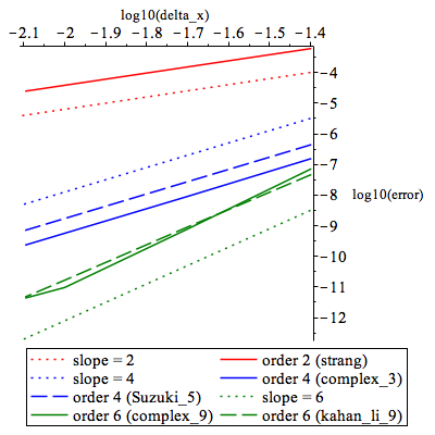
We observe that the schemes indeed produce the expected accuracy.

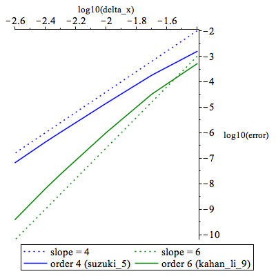
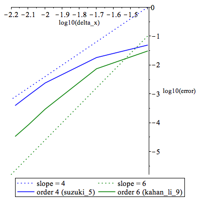
We make the same experiment with $\beta=50$. For this choice of CFL number, we found that the complex time step methods are unstable. The other methods are stable. The convergence study for the Suzuki and Kahan-Li schemes is presented on Figure 2.

Figure 2: Convergence study for palindromic methods at order 4 (blue, Suzuki scheme) and 6 (green, Kahan-Li scheme) with high CFL number $\beta=50$. The dotted lines are reference lines with slopes 4 and 6 respectively. We observe that the schemes are stable and that for sufficiently fine meshes, the expected rates of convergence are attained.

7.2 Behavior for discontinuous solutions

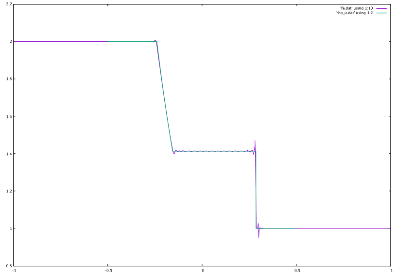
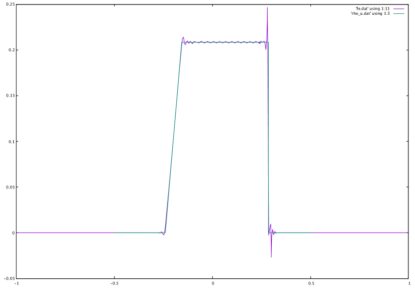
We have also experimented the scheme with complex time steps for discontinuous solutions. Of course, in this case the effective order of the method cannot be higher than one and we expect Gibbs oscillations near the discontinuities. On the interval $[a,b]=[-1,1],$ we consider a Riemann problem with the following initial condition

$$\rho(x,0)=\begin{cases}2&\text{if }x<0,\\ 1&\text{otherwise.}\end{cases},\quad u(x,0)=0.$$

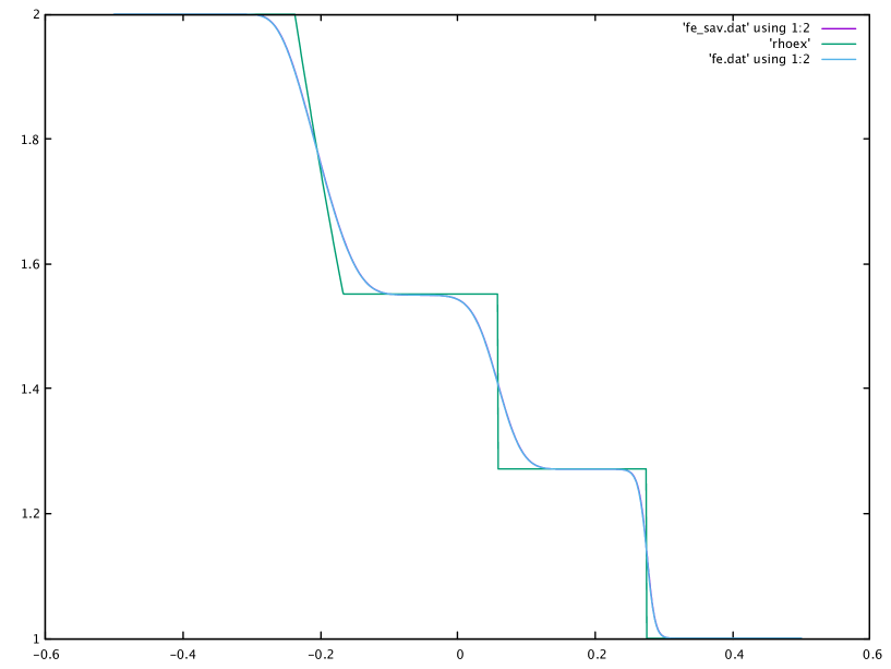
We consider numerical results in the fluid limit $\tau=0$. On Figure 3 we compare the sixth-order numerical solution with the exact one for a CFL number $\beta=3$ and $N_{x}=100$ cells. We observe that the high order scheme is able to capture a precise rarefaction wave and the correct position of the shock wave. We observe oscillations in the shock wave as expected.

Figure 3: Riemann problem with $\tau=0$. Comparison of the exact density (green curve), and the numerical sixth-order solution with complex time steps (purple curve). The number of DG cells is $N_{x}=100$ and the CFL number $\beta=3$.

Figure 4: Riemann problem with $\tau=0$. Comparison of the exact velocity (green curve), and the numerical sixth-order solution with complex time steps (purple curve). The number of DG cells is $N_{x}=100$ and the CFL number $\beta=3$.

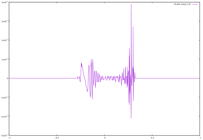
The complex time step method is used for approximating the real solution of a differential equation. We thus expect that the imaginary part of the numerical solution is small. We plot the imaginary part of $\rho$ on Figure 5. We observe that the imaginary part is indeed small (of the order $10^{-5}$) and that it takes its higher values in the discontinuous region. Maybe that it could be used as a shock indicator for detecting oscillations and controlling them.

Figure 5: Riemann problem with $\tau=0$. Imaginary part of the numerical density. We observe that it is of order $10^{-5}$ and that it has higher variations near to the shock. Maybe that it could be used as an error indicator.

7.3 Low Mach flow

In this section, we consider the Euler equations for a compressible gas with polytropic exponent $\gamma=7/5$. The primitive unknowns are the density $\rho$, the velocity $u$ and the pressure $p$. The conservative system is given by

$$w=(\rho,\rho u,\frac{1}{2}\rho u^{2}+\frac{p}{\gamma-1}),\quad q(w)=(\rho u,\rho u^{2}+p,\frac{1}{2}\rho u^{3}+\frac{\gamma pu}{\gamma-1}).$$ (25)

The eigenvalues of $D_{w}q(w)$ are

$$\mu_{1}=u-c,\quad\mu_{2}=u,\quad\mu_{3}=u+c,\quad\text{ with }c=\sqrt{\frac{\gamma p}{\rho}}.$$

We consider the following exact solution

$$u=\frac{1}{100},\quad p=1,\quad\rho=\omega\rho_{L}+(1-\omega)\rho_{R},$$

with

$$\rho_{L}=2,\quad\rho_{R}=1,\quad\omega=\left(1-\text{erf}(10(x-ut))\right)/2.$$

It represents a smooth and slowly moving contact wave. We compare the exact and numerical solutions at time $t=20$ with a CFL number $\beta=100$ and $\lambda=2$. The convergence study is presented on Figure 6. We observe the expected convergence rates. For such CFL number $\beta$, the schemes with complex time steps are unstable.

Figure 6: Convergence study for the low Mach test case with a CFL number $\beta=100$. Comparison of the fourth-order Suzuki scheme (blue) and the sixth-order Kahan-Li scheme (green). The dotted lines are reference lines with slopes 4 and 6 respectively. We observe the expected convergence rates for fine enough meshes. With this CFL number, the schemes with complex time steps are unstable.

7.4 Viscous test

In the above tests, we have assumed infinitely fast relaxation $\tau=0$. In this subsection we present a test with $\tau>0$. In practice the relaxation schemes are generally used with small relaxation time $\tau$. Indeed, with Taylor or Chapman-Enskog expansions, it is possible to prove that the relaxation scheme is, at order $O(\tau^{2})$, an approximation of

$$\partial_{t}w+\partial_{x}q(w)-\tau\partial_{x}B\partial_{x}w=0,$$

where the matrix $B$ depends on the choice of the lattice velocities, Maxwellian states, etc. To some extent it is possible to adjust $B$ to real physical terms, such as the Navier-Stokes viscosity (on this subject, see for instance [8, 27, 11]). The higher order terms in $\tau$ involve higher order space derivatives, which are generally undesirable. The smallness of $\tau$ implies that, in practice, it is important to handle the cases $\tau<\Delta t$ or $\tau\approx\Delta t$.

We consider the Euler model (25) with $x\in[-1/2,1/2]$, $t\in[0,0.2]$ and the following initial condition

$$w(x,0)=\begin{cases}w_{L}&\text{if }x<0,\\ w_{R}&\text{otherwise.}\end{cases}$$

The left and right states are given by

$$w_{L}=(2,0,5),\quad w_{R}=(1,0,5/2).$$

We consider the sixth-order Kahan-Li scheme (23) with a mesh of size $N_{x}=100$ and a CFL number $\beta=5$.

We have already observed that the collision step (13) cannot be applied if $2\tau+\gamma_{2}\Delta t/2=0$ (the $\Delta t/2$ comes from the definition of the elementary brick (17)). In this way we find a critical value of $\tau=\tau_{c}=0.000519$ for which the Kahan-Li scheme is unusable. With the same parameters, we have found that the five-step Suzuki scheme (22) is unstable.

However, the sixth-order scheme with complex time steps (20) is stable. The resulting density is plot on Figure 7. On the same figure we also represent a computation on a finer mesh with $N_{x}=1000$ cells. The curves with $N_{x}=100$ and $N_{x}=1000$ are indistinguishable (the error in the $L^{2}$ norm is of the order of $10^{-4}).$

If we take a higher CFL number $\beta=10,$ we then observe that the Kahan-Li scheme becomes stable again and produces results that are very similar to those of Figure 7.

Figure 7: Riemann problem with $\tau=0.000519$. Comparison of the exact density of the inviscid case (green curve), and the sixth-order complex numerical solution with $\tau>0$ (blue and purple curves: indistinguishable). The number of DG cells is $N_{x}=100$ or $N_{x}=1000$ and the CFL number $\beta=5$. The relaxation parameter has the same effect as a viscosity parameter.

The conclusion of this numerical test is that it is possible to compute with high precision the solution of the relaxation system when $\tau>0$. However, the stability conditions of the different schemes are for the moment unclear. It seems that it is possible to cross the “$2\tau+\Delta t$ barrier” if we consider the complex method at moderate CFL numbers $\beta.$

8 Conclusion

In this paper we have described a new numerical method, the Palindromic Discontinuous Galerkin Lattice Boltzmann Method, for solving kinetic equations with stiff relaxation. The method has the following features:

• Time integration is high order, based on a general palindromic composition method. We have tested it at order $4$ and $6$.

• The transport solver is based on an implicit high order upwind Discontinuous Galerkin method. Thanks to the upwind flux, the linear system to be solved at each time step is triangular.

• The scheme has better stability properties than an explicit scheme and allows for low storage optimization.

• The method is general, highly parallel and can be extended to higher dimensions.

We are currently working on the extension of the method to higher dimensions and to optimizations of the implementation on hybrid computers. A lot of theoretical and numerical investigations are still needed for understanding the stability properties of the method. It is also important in practical applications to extend the method with more general boundary conditions.

Bibliography

- [1] Jürgen Bey and Gabriel Wittum. Downwind numbering: Robust multigrid for convection-diffusion problems. Applied Numerical Mathematics, 23(1):177–192, 1997.
- [2] François Castella, Philippe Chartier, Stéphane Descombes, and Gilles Vilmart. Splitting methods with complex times for parabolic equations. BIT Numerical Mathematics, 49(3):487–508, 2009.
- [3] Shiyi Chen and Gary D Doolen. Lattice Boltzmann method for fluid flows. Annual review of fluid mechanics, 30(1):329–364, 1998.
- [4] Frédéric Coquel, Q-L Nguyen, Marie Postel, and Q-H Tran. Large time step positivity-preserving method for multiphase flows. In Hyperbolic Problems: Theory, Numerics, Applications, pages 849–856. Springer, 2008.
- [5] Timothy A Davis and Ekanathan Palamadai Natarajan. Algorithm 907: KLU, a direct sparse solver for circuit simulation problems. ACM Transactions on Mathematical Software (TOMS), 37(3):36, 2010.
- [6] Paul J Dellar. An interpretation and derivation of the lattice Boltzmann method using Strang splitting. Computers & Mathematics with Applications, 65(2):129–141, 2013.
- [7] François Dubois. Stable lattice Boltzmann schemes with a dual entropy approach for monodimensional nonlinear waves. Computers & Mathematics with Applications, 65(2):142–159, 2013.
- [8] François Dubois, Benjamin Graille, and Pierre Lallemand. Recovering the full Navier-Stokes equations with lattice Boltzmann schemes. In 30th international symposium on rarefied gas dynamics: rgd 30, volume 1786, page 040003. AIP Publishing, 2016.
- [9] Benjamin Graille. Approximation of mono-dimensional hyperbolic systems: A lattice Boltzmann scheme as a relaxation method. Journal of Computational Physics, 266:74–88, 2014.
- [10] Ernst Hairer, Christian Lubich, and Gerhard Wanner. Geometric numerical integration: structure-preserving algorithms for ordinary differential equations, volume 31. Springer Science & Business Media, 2006.
- [11] Xiaoyi He and Li-Shi Luo. Lattice Boltzmann model for the incompressible Navier–Stokes equation. Journal of statistical Physics, 88(3-4):927–944, 1997.
- [12] Philippe Helluy. Stability analysis of an implicit lattice Boltzmann scheme. To appear in Oberwolfach reports. https://hal.archives-ouvertes.fr/hal-01403759, 2016.
- [13] Jan S Hesthaven and Tim Warburton. Nodal discontinuous Galerkin methods: algorithms, analysis, and applications. Springer Science & Business Media, 2007.
- [14] Willem Hundsdorfer and Jan G Verwer. Numerical solution of time-dependent advection-diffusion-reaction equations, volume 33. Springer Science & Business Media, 2013.
- [15] Shi Jin. Runge-Kutta methods for hyperbolic conservation laws with stiff relaxation terms. Journal of Computational Physics, 122(1):51–67, 1995.
- [16] Shi Jin. Efficient asymptotic-preserving (AP) schemes for some multiscale kinetic equations. SIAM Journal on Scientific Computing, 21(2):441–454, 1999.
- [17] Shi Jin and Zhouping Xin. The relaxation schemes for systems of conservation laws in arbitrary space dimensions. Communications on pure and applied mathematics, 48(3):235–276, 1995.
- [18] William Kahan and Ren-Cang Li. Composition constants for raising the orders of unconventional schemes for ordinary differential equations. Mathematics of Computation of the American Mathematical Society, 66(219):1089–1099, 1997.
- [19] Tai-Ping Liu. Hyperbolic conservation laws with relaxation. Communications in Mathematical Physics, 108(1):153–175, 1987.
- [20] Robert I McLachlan and G Reinout W Quispel. Splitting methods. Acta Numerica, 11:341–434, 2002.
- [21] Renwei Mei and Wei Shyy. On the finite difference-based lattice Boltzmann method in curvilinear coordinates. Journal of Computational Physics, 143(2):426–448, 1998.
- [22] Misun Min and Taehun Lee. A spectral-element Discontinuous Galerkin lattice Boltzmann method for nearly incompressible flows. Journal of Computational Physics, 230(1):245–259, 2011.
- [23] Salli Moustafa, Mathieu Faverge, Laurent Plagne, and Pierre Ramet. 3D cartesian transport sweep for massively parallel architectures with PARSEC. In Parallel and Distributed Processing Symposium (IPDPS), 2015 IEEE International, pages 581–590. IEEE, 2015.
- [24] Francesca Nannelli and Sauro Succi. The lattice Boltzmann equation on irregular lattices. Journal of Statistical Physics, 68(3-4):401–407, 1992.
- [25] Jostein R Natvig and Knut-Andreas Lie. Fast computation of multiphase flow in porous media by implicit discontinuous galerkin schemes with optimal ordering of elements. Journal of Computational Physics, 227(24):10108–10124, 2008.
- [26] Gongwen Peng, Haowen Xi, Comer Duncan, and So-Hsiang Chou. Lattice Boltzmann method on irregular meshes. Physical Review E, 58(4):R4124, 1998.
- [27] YH Qian, Dominique d’Humières, and Pierre Lallemand. Lattice BGK models for Navier-Stokes equation. EPL (Europhysics Letters), 17(6):479, 1992.
- [28] Xing Shi, Jianzhong Lin, and Zhaosheng Yu. Discontinuous Galerkin spectral element lattice Boltzmann method on triangular element. International Journal for Numerical Methods in Fluids, 42(11):1249–1261, 2003.
- [29] Masuo Suzuki. Fractal decomposition of exponential operators with applications to many-body theories and monte carlo simulations. Physics Letters A, 146(6):319–323, 1990.
- [30] Feng Wang and Jinchao Xu. A crosswind block iterative method for convection-dominated problems. SIAM Journal on Scientific Computing, 21(2):620–645, 1999.
- [31] Gerald B Witham. Linear and Non-linear Waves. Wiley, 1974.