Uniform infinite half-planar quadrangulations with skewness

Abstract

We introduce a one-parameter family of random infinite quadrangulations of the half-plane, which we call the uniform infinite half-planar quadrangulations with skewness ($\textup{{UIHPQ}}_{p}$ for short, with $p\in[0,1/2]$ measuring the skewness). They interpolate between Kesten’s tree corresponding to $p=0$ and the usual UIHPQ with a general boundary corresponding to $p=1/2$. As we make precise, these models arise as local limits of uniform quadrangulations with a boundary when their volume and perimeter grow in a properly fine-tuned way, and they represent all local limits of (sub)critical Boltzmann quadrangulations whose perimeter tend to infinity. Our main result shows that the family $(\textup{{UIHPQ}}_{p})_{p}$ approximates the Brownian half-planes $\textup{{BHP}}_{\theta}$, $\theta\geq 0$, recently introduced in [8]. For $p<1/2$, we give a description of the $\textup{{UIHPQ}}_{p}$ in terms of a looptree associated to a critical two-type Galton-Watson tree conditioned to survive.

Key words: Uniform infinite half-planar quadrangulation, Brownian half-plane, Kesten’s tree, multi-type Galton-Watson tree, looptree, Boltzmann map.
Subject Classification: 05C80; 05C81; 05C05; 60J80; 60F05.

1 Introduction

1.1 Overview

The purpose of this paper is to introduce and study a one-parameter family of random infinite quadrangulations of the half-plane, which we denote by $(\textup{{UIHPQ}}_{p})_{0\leq p\leq 1/2}$ and call the uniform infinite half-planar quadrangulations with skewness. Two members play a particular role: The choice $p=0$ corresponds to Kesten’s tree, cf. Proposition 1 below, whereas the choice $p=1/2$ corresponds to the standard uniform infinite half-planar quadrangulation UIHPQ with a general boundary.

Kesten’s tree [31] is a random infinite planar tree, which we may view as a degenerate quadrangulation with an infinite boundary, but no inner faces. It arises as the local limit of critical Galton-Watson trees conditioned to survive. The standard $\textup{{UIHPQ}}(=\textup{{UIHPQ}}_{1/2})$ forms the half-planar analog of the uniform infinite planar quadrangulation introduced by Krikun [32], after the seminal work of Angel and Schramm [7] on triangulations of the plane. Curien and Miermont [25] showed that the UIHPQ arises as a local limit of uniformly chosen quadrangulations of the two-sphere with $n$ inner faces and a boundary of size $2\sigma$, upon letting first $n\rightarrow\infty$ and then $\sigma\rightarrow\infty$ (see Angel [3] for the case of triangulations with a simple boundary).

We will define each $\textup{{UIHPQ}}_{p}$ in Section 4 by means of an extension of the Bouttier-Di Francesco-Guitter mapping to infinite quadrangulations with a boundary. In the first part of this paper, we will discuss various local limits and scaling limits which involve the family $(\textup{{UIHPQ}}_{p})_{p}$. More precisely, in Theorem 1, we will see that each $\textup{{UIHPQ}}_{p}$ appears as a local limit as $n$ tends to infinity of uniform quadrangulations $Q_{n}^{\sigma_{n}}$ with $n$ inner faces and a boundary of size $2\sigma_{n}$, for an appropriate choice of $\sigma_{n}=\sigma_{n}(p)\rightarrow\infty$. In Proposition 2, we argue that the family $(\textup{{UIHPQ}}_{p})_{p}$ consists precisely of the infinite quadrangulations with a boundary which are obtained as local limits $\sigma\rightarrow\infty$ of subcritical Boltzmann quadrangulations with a boundary of size $2\sigma$. This result will prove helpful in our description of the $\textup{{UIHPQ}}_{p}$ given in Theorem 4.

We will then turn to distributional scaling limits of the family $(\textup{{UIHPQ}}_{p})_{p}$ in the so-called local Gromov-Hausdorff topology. In Theorems 2 and 3, we will clarify the connection between the (discrete) quadrangulations $\textup{{UIHPQ}}_{p}$ and the family $(\textup{{BHP}}_{\theta})_{\theta\geq 0}$ of Brownian half-spaces with skewness $\theta$ introduced in [8]. More specifically, upon rescaling the graph distance by a factor $a_{n}^{-1}\rightarrow 0$, we prove that each $\textup{{BHP}}_{\theta}$ is the distributional limit of the rescaled spaces $a_{n}^{-1}\cdot\textup{{UIHPQ}}_{p_{n}}$, if $p_{n}=p_{n}(\theta,a_{n})$ is adjusted in the right manner (Theorem 2). In our setting, convergence in the local Gromov-Hausdorff sense amounts to show convergence of rescaled metric balls around the roots of a fixed but arbitrarily large radius in the usual Gromov-Hausdorff topology; see Section 1.2.7.

In [8], a classification of all possible non-compact scaling limits of pointed uniform random quadrangulations with a boundary $(V(Q_{n}^{\sigma_{n}}),a_{n}^{-1}d_{\textup{gr}},\rho_{n})$ has been given, depending on the asymptotic behavior of the boundary size $2\sigma_{n}$ and on the choice of the scaling factor $a_{n}\rightarrow\infty$ (in the local Gromov-Hausdorff topology, with the distinguished point $\rho_{n}$ lying on the boundary). In this paper, we address the boundary regime corresponding to the portion $x\geq 1$ of the $y=0$ axis in Figure 1 (in hashed marks), which was left untouched in [8]. As we show, it corresponds to a regime of unrescaled local limits, namely the family $(\textup{{UIHPQ}}_{p})_{p}$.

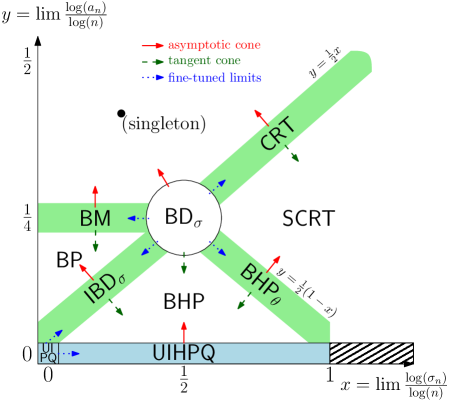
Figure 1: In [8], all possible limits for the rescaled spaces $(V(Q_{n}^{\sigma_{n}}),a_{n}^{-1}d_{\textup{gr}},\rho_{n})$ are discussed. The $x$-axis represents the limit values for the logarithm of the boundary length $\log(\sigma_{n})/\log(n)$ in units of $\log(n)$, and the $y$-axis corresponds to the limit of the logarithm of the scaling factor $\log(a_{n})/\log(n)$ in units of $\log(n)$. The focus of this paper lies on the hashed region.

We finally give a branching characterization of the $\textup{{UIHPQ}}_{p}$ when $p<1/2$. For that purpose, we will adapt the concept of discrete random looptrees introduced by Curien and Kortchemski [22]. We will see that the $\textup{{UIHPQ}}_{p}$ admits a representation in terms of a looptree associated to a two-type version of Kesten’s infinite tree. Informally, we will replace each vertex $u$ at odd height in Kesten’s tree by a cycle of length $\deg(u)$, which connects the vertices incident to $u$. Here, $\deg(u)$ stands for the degree (i.e., the number of neighbors) of $u$ in the tree. We then fill in the cycles of the looptree with a collection of independent quadrangulations with a simple boundary, which are drawn according to a subcritical Boltzmann law. As we show in Theorem 4, the space constructed in this way has the law of the $\textup{{UIHPQ}}_{p}$. Discrete looptrees and their scaling limits have found various applications in the study of large-scale properties of random planar maps, for instance in the description of the boundary of percolation clusters on the uniform infinite planar triangulation; see the work [23], which served as the main inspiration for our characterization of the $\textup{{UIHPQ}}_{p}$. From our description, we immediately infer that simple random walk is recurrent on the $\textup{{UIHPQ}}_{p}$ for $p<1/2$.

It is well-known that the standard UIHPQ with a simple boundary satisfies the so-called spatial Markov property, which allows, in particular, the use of peeling techniques. In [5], Angel and Ray classified all triangulations (without self-loops) of the half-plane satisfying the spatial Markov property and translation invariance. They form a one-parameter family $(\mathbb{H}_{\alpha})_{\alpha}$ parametrized by $\alpha\in[0,1)$. The parameter $\alpha=2/3$ corresponds to the standard UIHPT with a simple boundary, the triangular equivalent of the UIHPQ with a simple boundary. When $\alpha>2/3$ (the supercritical case), $\mathbb{H}_{\alpha}$ is of hyperbolic nature and exhibits an exponential volume growth. On the contrary, when $\alpha<2/3$ (the subcritical case), it has a tree-like structure. We believe that the family $(\textup{{UIHPQ}}_{p})_{p}$ is a quadrangular equivalent to the triangulations in the subcritical phase of [5]. Note that contrary to the $\textup{{UIHPQ}}_{p}$, the spaces $\mathbb{H}_{\alpha}$ for $\alpha<2/3$ have a half-plane topology, due to the conditioning to have a simple boundary. However, there exists almost surely infinitely many cut-edges connecting the left and right boundaries; see [38, Proposition 4.11]. This should be seen as an equivalent to the branching structure formulated in Theorem 4 below. Our methods in this paper are different from [5, 38] as we do not use peeling techniques.

In [21], Curien studied full-plane analogs of the family $(\mathbb{H}_{\alpha})_{\alpha}$. With similar (peeling) techniques, he constructed a (unique) one-parameter family of random infinite planar triangulations indexed by $\kappa\in(0,2/27]$, which satisfy a slightly adapted spatial Markov property. The critical case $\kappa=2/27$ corresponds to the standard UIPT with a simple boundary of Angel and Schramm [7]. The regime $\kappa\in(0,2/27)$ parallels the supercritical (or hyperbolic) phase $\alpha>2/3$ of [5], whereas it is shown that there is no subcritical phase. Recently, a near-critical scaling limit of hyperbolic nature called the hyperbolic Brownian half-plane has been studied by Budzinski [17]. It is obtained from rescaling the triangulations of Curien [21] and letting $\kappa\rightarrow 2/27$ at the right speed. Theorem 1 of [17] bears some structural similarities with our Theorem 2 below, although it concerns a different regime.

Structure of the paper
The rest of this paper is structured as follows. In the following section, we introduce some (standard) concepts and notation around quadrangulations, which will be used throughout this text. Moreover, we recapitulate the local topology and the local Gromov-Hausdorff topology. In Section 2, we state our main results, which concern local limits, scaling limits, and structural properties of the family $(\textup{{UIHPQ}}_{p})_{p}$. Section 3 reviews the definition of the family of Brownian half-planes $(\textup{{BHP}}_{\theta})_{\theta}$, and of various random trees, which are used both to describe the distributional limits of the family $(\textup{{UIHPQ}}_{p})_{p}$ as well as their branching structure.

In Section 4, we construct the $\textup{{UIHPQ}}_{p}$. We first explain the Bouttier-Di Francesco-Guitter encoding of quadrangulations with a boundary and then define the $\textup{{UIHPQ}}_{p}$ in terms of the encoding objects. We are then in position to prove our limit statements; see Section 5. In the final Section 6, we prove our main result characterizing the tree-like structure of the $\textup{{UIHPQ}}_{p}$ when $p<1/2$, as well as recurrence of simple random walk.

1.2 Some standard notation and definitions

1.2.1 Notation

We write

$$\mathbb{N}=\{1,2,\ldots\},\quad\mathbb{N}_{0}=\mathbb{Z}_{\geq 0}=\mathbb{N}\cup\{0\},\quad\mathbb{Z}_{<0}=\{-1,-2,\ldots\}.$$

For two sequences $(a_{n})_{n}$, $(b_{n})_{n}\subset\mathbb{N}$, we write $a_{n}\ll b_{n}$ or $b_{n}\gg a_{n}$ if $a_{n}/b_{n}\rightarrow 0$ as $n\rightarrow\infty$. Given two measurable subsets $U,V\subset\mathbb{R}$, we denote by $\mathcal{C}(U,V)$ the space of continuous functions from $U$ to $V$, equipped with the usual compact-open topology, i.e., uniform convergence on compact subsets. We write $\|\nu\|_{\textup{TV}}$ for the total variation norm of a probability measure $\nu$.

As a general notational rule for this paper, if we drop $p$ from the notation, we work with the case $p=1/2$. For example, we write UIHPQ (and not $\textup{{UIHPQ}}_{1/2}$) for the standard uniform infinite half-planar quadrangulation.

1.2.2 Planar maps

By planar map we mean, as usual, an equivalence class of a proper embedding of a finite connected graph in the two-sphere, where two embeddings are declared to be equivalent if they differ only by an orientation-preserving homeomorphism of the sphere. Loops and multiple edges are allowed. Our planar maps will be rooted, meaning that we distinguish an oriented edge called the root edge. Its origin is the root vertex of the map. The faces of a planar map are formed by the components of the complement of the union of its edges.

1.2.3 Quadrangulations with a boundary

A quadrangulation with a boundary is a finite planar map $\mathsf{q}$, whose faces are quadrangles except possibly one face called the outer face, which may an have arbitrary even degree. The edges incident to the outer face form the boundary $\partial\textup{$\mathsf{q}$}$ of $\mathsf{q}$, and their number $\#\partial\textup{$\mathsf{q}$}$ (counted with multiplicity) is the size or perimeter of the boundary. In general, we do not assume that the boundary edges form a simple curve. We will root the map by selecting an oriented edge of the boundary, such that the outer face lies to its right. The size of $\mathsf{q}$ is given by the number of its inner faces, i.e., all the faces different from the outer face.

We write $\mathcal{Q}_{n}^{\sigma}$ for the (finite) set of all rooted quadrangulations with $n$ inner faces and a boundary of size $2\sigma$, $\sigma\in\mathbb{N}_{0}$. By convention, $\mathcal{Q}_{0}^{0}=\{{\dagger}\}$ consists of the unique vertex map.

More generally, $\mathcal{Q}_{f}$ will denote the set of all finite rooted quadrangulations with a boundary, and $\mathcal{Q}^{\sigma}_{f}\subset\mathcal{Q}_{f}$ the set of all finite rooted quadrangulations with $2\sigma$ boundary edges, for $\sigma\in\mathbb{N}_{0}$.

Similarly, we let $\widehat{\mathcal{Q}}_{f}$ be the set of all finite rooted quadrangulations with a simple boundary, meaning that the edges of their outer face form a cycle without self-intersection. We denote by $\widehat{\mathcal{Q}}^{\sigma}_{f}\subset\widehat{\mathcal{Q}}_{f}$ the subset of finite rooted quadrangulations with a simple boundary of size $2\sigma$. Note that $\mathcal{Q}_{0}^{1}$ consists of the map having one oriented edge and thus a simple boundary.

1.2.4 Uniform quadrangulations with a boundary

Throughout this text, we write $Q_{n}^{\sigma}$ for a quadrangulation chosen uniformly at random in $\mathcal{Q}_{n}^{\sigma}$. We denote by $\rho_{n}$ the root vertex of $Q_{n}^{\sigma}$, i.e., the origin of the root edge. By equipping the set of vertices $V(Q_{n}^{\sigma})$ with the graph distance $d_{\textup{gr}}$, we view the triplet $(V(Q_{n}^{\sigma}),d_{\textup{gr}},\rho_{n})$ as a random rooted metric space.

1.2.5 Boltzmann quadrangulations with a boundary

We will also work with various Boltzmann measures. For a finite rooted quadrangulation $\textup{$\mathsf{q}$}\in\mathcal{Q}_{f}$, we write $\textup{F}(\textup{$\mathsf{q}$})$ for the set of inner faces of $\mathsf{q}$. Given non-negative weights $g$ per inner face and $\sqrt{z}$ per boundary edge, we let

$$F(g,z)=\sum_{\textup{$\mathsf{q}$}\in\mathcal{Q}_{f}}g^{\#\textup{F}(\textup{$\mathsf{q}$})}z^{\#\partial\textup{$\mathsf{q}$}/2}.$$

When this partition function is finite, we may define the associated Boltzmann distribution

$$\mathbb{P}_{g,z}(\textup{$\mathsf{q}$})=\frac{g^{\#\textup{F}(\textup{$\mathsf{q}$})}z^{\#\partial\textup{$\mathsf{q}$}/2}}{F(g,z)},\quad\textup{$\mathsf{q}$}\in\mathcal{Q}_{f}.$$

The statement of Proposition 2 below deals with Boltzmann-distributed quadrangulations of a fixed boundary size $2\sigma$, for $\sigma\in\mathbb{N}_{0}$. In this case, the associated partition function and Boltzmann distribution read

$$F_{\sigma}(g)=\sum_{\textup{$\mathsf{q}$}\in\mathcal{Q}^{\sigma}_{f}}g^{\#\textup{F}(\textup{$\mathsf{q}$})},\quad\mathbb{P}^{\sigma}_{g}(\textup{$\mathsf{q}$})=\frac{g^{\#\textup{F}(\textup{$\mathsf{q}$})}}{F_{\sigma}(g)},\quad\textup{$\mathsf{q}$}\in\mathcal{Q}^{\sigma}_{f},$$

whenever $g\geq 0$ is such that $F_{\sigma}(g)$ is finite. The Boltzmann distribution $\mathbb{P}^{\sigma}_{g}$ is related to $\mathbb{P}_{g,z}$ by conditioning the latter with respect to the boundary length, i.e., $\mathbb{P}^{\sigma}_{g}(\textup{$\mathsf{q}$})=\mathbb{P}_{g,z}(\textup{$\mathsf{q}$}\mid\mathcal{Q}^{\sigma}_{f})$.

When studying quadrangulations with a simple boundary, the partition functions are

$$\widehat{F}(g,z)=\sum_{\textup{$\mathsf{q}$}\in\widehat{\mathcal{Q}}_{f}}g^{\#\textup{F}(\textup{$\mathsf{q}$})}z^{\#\partial\textup{$\mathsf{q}$}/2},\quad\widehat{F}_{\sigma}(g)=\sum_{\textup{$\mathsf{q}$}\in\widehat{\mathcal{Q}}^{\sigma}_{f}}g^{\#\textup{F}(\textup{$\mathsf{q}$})},$$

and the Boltzmann distributions take the form

$$\widehat{\mathbb{P}}_{g,z}(\textup{$\mathsf{q}$})=\frac{g^{\#\textup{F}(\textup{$\mathsf{q}$})}}{\widehat{F}_{\sigma}(g,z)},\quad\textup{$\mathsf{q}$}\in\widehat{\mathcal{Q}}_{f},\quad\widehat{\mathbb{P}}^{\sigma}_{g}(\textup{$\mathsf{q}$})=\frac{g^{\#\textup{F}(\textup{$\mathsf{q}$})}}{\widehat{F}_{\sigma}(g)},\quad\textup{$\mathsf{q}$}\in\widehat{\mathcal{Q}}^{\sigma}_{f}.$$

Remark 1.

In the notation of [15], the generating function $F$ is denoted $W_{0}$, while $\widehat{F}$ is denoted $\tilde{W}_{0}$. The index zero stands for the distance between the origin of the root edge and the marked vertex, so that these generating functions count unpointed quadrangulations.

1.2.6 Local topology

Our unrescaled limit results hold with respect to the local topology first studied by Benjamini and Schramm [10]: For two rooted planar maps m and $\textup{{m}}^{\prime}$, the local distance between m and $\textup{{m}}^{\prime}$ is

$$d_{\textup{map}}(\textup{{m}},\textup{{m}}^{\prime})=\left(1+\sup\{r\geq 0:\textup{Ball}_{r}(\textup{{m}})=\textup{Ball}_{r}(\textup{{m}}^{\prime})\}\right)^{-1},$$

where $\textup{Ball}_{r}(\textup{{m}})$ denotes the combinatorial ball of radius $r$ around the root $\rho$ of m, i.e., the submap of m consisting of all the vertices $v$ of m with $d_{\textup{gr}}(\rho,v)\leq r$ and all the edges of m between such vertices. The set $\mathcal{Q}_{f}$ of all finite rooted quadrangulations with a boundary is not complete for the distance $d_{\textup{map}}$; we have to add infinite quadrangulations. We shall write $\mathcal{Q}$ for the completion of $\mathcal{Q}_{f}$ with respect to $d_{\textup{map}}$. The $\textup{{UIHPQ}}_{p}$ will be defined as a random element in $\mathcal{Q}$.

1.2.7 Around the Gromov-Hausdorff metric

The pointed Gromov-Hausdorff distance measures the distance between (pointed) compact metric spaces, where the latter are viewed up to isometries. More specifically, given two elements $\mathbf{E}=(E,d,\rho)$ and $\mathbf{E}^{\prime}=(E^{\prime},d^{\prime},\rho^{\prime})$ in the space $\mathbb{K}$ of isometry classes of pointed compact metric spaces, their Gromov-Hausdorff distance is defined as

$$d_{\textup{GH}}(\mathbf{E},\mathbf{E}^{\prime})=\inf\left\{d_{\textup{H}}(\varphi(E),\varphi^{\prime}(E))\vee\delta(\varphi(\rho),\varphi^{\prime}(\rho^{\prime}))\right\},$$

where the infimum is taken over all isometric embeddings $\varphi:E\rightarrow F$ and $\varphi^{\prime}:E^{\prime}\rightarrow F$ of $E$ and $E^{\prime}$ into the same metric space $(F,\delta)$, and $d_{\textup{H}}$ is the usual Hausdorff distance between compacts of $F$. The space $(\mathbb{K},d_{\textup{GH}})$ is complete and separable.

Our results on scaling limits involve non-compact pointed metric spaces and hold in the so-called local Gromov-Hausdorff sense, which we briefly recall next. Given a pointed complete and locally compact length space $\mathbf{E}$ and a sequence $(\mathbf{E}_{n})_{n}$ of such spaces, $(\mathbf{E}_{n})_{n}$ converges in the local Gromov-Hausdorff sense to $\mathbf{E}$ if for every $r\geq 0$,

$$d_{\textup{GH}}(B_{r}(\mathbf{E}_{n}),B_{r}(\mathbf{E}))\rightarrow 0\quad\textup{ as }n\rightarrow\infty.$$

Here and in what follows, given a pointed metric space $\mathbf{F}=(F,d,\rho)$, $B_{r}(\mathbf{F})=\{x\in F:d(x,\rho)\leq r\}$ denotes the closed ball of radius $r$ around $\rho$, viewed as a subspace of $\mathbf{F}$ equipped with the metric structure inherited from $\mathbf{F}$. For $\lambda>0$, $\lambda\cdot\mathbf{F}$ stands for the rescaled pointed metric space $(F,\lambda d,\rho)$, so that in particular $\lambda\cdot B_{r}(\mathbf{F})=B_{\lambda r}(\lambda\cdot\mathbf{F})$.

As a discrete map, the $\textup{{UIHPQ}}_{p}$ is not a length space in the sense of [18]. However, by identifying each edge with a copy of the unit interval $[0,1]$ (and by extending the metric isometrically), one obtains a complete locally compact length space (pointed at the root vertex). By construction, balls of the same radius and around the same points in the $\textup{{UIHPQ}}_{p}$ and in the approximating length space are at Gromov-Hausdorff distance at most $1$ from each other. Therefore, local Gromov-Hausdorff convergence for the (rescaled) $\textup{{UIHPQ}}_{p}$, see Theorems 2 and 3 below, follows indeed from the convergence of balls as stated above.

2 Statements of the main results

2.1 Local limits

Our first result states that each member of the family $(\textup{{UIHPQ}}_{p})_{0\leq p\leq 1/2}$ can be seen as a local limit $n\rightarrow\infty$ of uniform quadrangulations of with $n$ inner faces and a boundary of size $2\sigma_{n}$, provided $\sigma_{n}=\sigma_{n}(p)$ is chosen in the right manner.

Theorem 1.

Fix $0\leq p\leq 1/2$, and let $(\sigma_{n},n\in\mathbb{N})$ be a sequence of positive integers satisfying

$$\sigma_{n}=\frac{1-2p}{p}n+o(n)\quad\textup{if }0<p\leq 1/2,\quad\textup{and}\quad\sigma_{n}\gg n\quad\textup{if }p=0.$$

For every $n\in\mathbb{N}$, let $Q_{n}^{\sigma_{n}}$ be uniformly distributed in $\mathcal{Q}_{n}^{\sigma_{n}}$. Then we have the local convergence for the metric $d_{\textup{map}}$ as $n\rightarrow\infty$,

$$Q_{n}^{\sigma_{n}}\xrightarrow[]{(d)}\textup{{UIHPQ}}_{p}.$$

In fact, we will prove a stronger result than mere local convergence: We will establish an isometry of balls of growing radii around the roots, where the maximal growth rate of the radii is given by $\xi_{n}=o(\sqrt{n})$. We defer to Proposition 4 for the exact statement. The case $p=1/2$ corresponding to the regime $\sigma_{n}=o(n)$ is already covered by [8, Proposition 3.11] and is only included for completeness.

The convergence in the case $p=0$ with $\sigma_{n}\gg n$ is somewhat simpler. However, it is a priori not obvious that the $\textup{{UIHPQ}}_{0}$ as defined in Section 4 is actually Kesten’s tree (see Section 3.2.3 for a definition of the latter).

Proposition 1.

The space $\textup{{UIHPQ}}_{0}$ has the law of Kesten’s tree $\mathcal{T}_{\infty}$ associated to the critical geometric probability distribution $(\mu_{1/2}(k),k\in\mathbb{N}_{0})$ given by $\mu_{1/2}(k)=2^{-(k+1)}$.

Interestingly, the fact that the $\textup{{UIHPQ}}_{0}$ is Kesten’s tree can also be derived as a special case from Theorem 4 below; see Remark 5. We prefer, however, to give a direct proof of the proposition based on our construction of the $\textup{{UIHPQ}}_{0}$.

The $\textup{{UIHPQ}}_{p}$ for $0\leq p\leq 1/2$ is also obtained as a local limit of Boltzmann quadrangulations with growing boundary size. This result will be important to describe the tree-like structure of the $\textup{{UIHPQ}}_{p}$ when $p<1/2$. More specifically, the family $(\textup{{UIHPQ}}_{p})_{p}$ is precisely given by the collection of all local limits $\sigma\rightarrow\infty$ of Boltzmann quadrangulations with a boundary of size $2\sigma$ and weight $g\leq g_{c}=1/12$ per inner face. The value $g_{c}=1/12$ is critical (see [15, Section 4.1]) and corresponds to the choice $p=1/2$.

Proposition 2.

Fix $0\leq p\leq 1/2$, and set $g_{p}=p(1-p)/3$. For every $\sigma\in\mathbb{N}_{0}$, let $Q_{\sigma}(p)$ be a random rooted quadrangulation distributed according to the Boltzmann measure $\mathbb{P}^{\sigma}_{g_{p}}$. Then we have the local convergence for the metric $d_{\textup{map}}$ as $\sigma\rightarrow\infty$,

$$Q_{\sigma}(p)\xrightarrow[]{(d)}\textup{{UIHPQ}}_{p}.$$

Remark 2.

For $p=1/2$, the above proposition states convergence of critical Boltzmann quadrangulations with a boundary towards the UIHPQ, as it was already proved in [20, Theorem 7] by means of peeling techniques. In view of the above proposition, it is moreover implicit from the same theorem that an infinite random map with the law of the $\textup{{UIHPQ}}_{p}$ does exist. For the case of half-planar triangulations (with a simple boundary), see [3]. When $p=0$, there is no inner quadrangle almost surely and $Q^{\sigma}(0)$ is a uniform tree with $\sigma$ edges (i.e., a Galton-Watson tree with geometric offspring law conditioned to have $\sigma$ edges), which converges locally towards Kesten’s tree; see, for example, [29, Theorem 7.1].

Remark 3.

Let us write $\mathcal{M}(\mathcal{Q})$ for the set of probability measures on the completion $\mathcal{Q}$, and equip it with the usual weak topology. Then it is easily seen by our methods that the mapping $[0,1/2]\ni p\mapsto\textup{Law}(\textup{{UIHPQ}}_{p})\in\mathcal{M}(\mathcal{Q})$ is continuous.

2.2 Scaling limits

Our next results address scaling limits of the family $(\textup{{UIHPQ}}_{p})_{p}$. In [8], a one-parameter family of (non-compact) random rooted metric spaces called the Brownian half-planes $\textup{{BHP}}_{\theta}$ with skewness $\theta\geq 0$ was introduced. See Section 3.1 for a quick reminder. The Brownian half-plane $\textup{{BHP}}_{0}$ corresponding to the choice $\theta=0$ forms the half-planar analog of the Brownian plane introduced in [24] and arises from zooming-out the UIHPQ around the root vertex; see [8, Theorem 3.6], and [27, Theorem 1.10]). Here, we will see more generally that the family $(\textup{{UIHPQ}}_{p})_{p}$ approximates the space $\textup{{BHP}}_{\theta}$ for each $\theta\geq 0$ in the local Gromov-Hausdorff sense, provided $p$ is appropriately fine-tuned (depending on $\theta$).

Theorem 2.

Let $\theta\geq 0$. Let $(a_{n},n\in\mathbb{N})$ be a sequence of positive reals with $a_{n}\rightarrow\infty$ as $n\rightarrow\infty$. Let $(p_{n},n\in\mathbb{N})\subset[0,1/2]$ be a sequence satisfying

$$p_{n}=p_{n}(\theta,a_{n})=\frac{1}{2}\left(1-\frac{2\theta}{3a_{n}^{2}}\right)+o\left(a_{n}^{-2}\right).$$

Then, in the sense of the local Gromov-Hausdorff topology as $n\rightarrow\infty$,

$$a_{n}^{-1}\cdot\textup{{UIHPQ}}_{p_{n}}\xrightarrow[]{(d)}\textup{{BHP}}_{\theta}.$$

The space $\textup{{BHP}}_{\theta}$ satisfies the scaling property $\lambda\cdot\textup{{BHP}}_{\theta}=_{d}\textup{{BHP}}_{\theta/\lambda^{2}}$. It was shown in Remark 3.19 of [8] that Aldous’ self-similar continuum random tree SCRT, whose definition is reviewed in Section 3.2.1, is the asymptotic cone of the $\textup{{BHP}}_{\theta}$ around its root, implying $\textup{{BHP}}_{\theta}\rightarrow\textup{{SCRT}}$ in law as $\theta\rightarrow\infty$. In particular, formally, we may think of the $\textup{{BHP}}_{\infty}$ as the SCRT. In view of Theorem 2, it is therefore natural to expect that the SCRT appears also as the scaling limit of the $\textup{{UIHPQ}}_{p_{n}}$, provided $\theta$ in the definition of $p_{n}$ is replaced by a sequence $\theta_{n}\rightarrow\infty$, that is, if $a_{n}^{2}(1-2p_{n})\rightarrow\infty$ as $n\rightarrow\infty$. This is indeed the case.

Theorem 3.

Let $(a_{n},n\in\mathbb{N})$ be a sequence of positive reals with $a_{n}\rightarrow\infty$. Let $(p_{n},n\in\mathbb{N})\subset[0,1/2]$ be a sequence satisfying

$$a_{n}^{2}(1-2p_{n})\rightarrow\infty\quad\textup{as }n\rightarrow\infty.$$

Then, in the sense of the local Gromov-Hausdorff topology as $n\rightarrow\infty$,

$$a_{n}^{-1}\cdot\textup{{UIHPQ}}_{p_{n}}\xrightarrow[]{(d)}\textup{{SCRT}}.$$

As special cases of the previous two theorems, we mention

Corollary 1.

Let $p\in[0,1/2]$, and let $(a_{n},n\in\mathbb{N})$ be a sequence of positive reals with $a_{n}\rightarrow\infty$. Then, in the sense of the local Gromov-Hausdorff topology as $n\rightarrow\infty$,

$$a_{n}^{-1}\cdot\textup{{UIHPQ}}_{p}\xrightarrow[]{(d)}\left\{\begin{array}[]{lcl}\textup{{SCRT}}&\mbox{ if }&0\leq p<1/2\\ \textup{{BHP}}&\mbox{ if }&p=1/2\end{array}\right..$$

For the family $(\mathbb{H}_{\alpha})_{\alpha}$ of half-planar triangulations studied in [5, 38], convergence towards the SCRT in the subcritical regime $\alpha<2/3$ is conjectured in [38, Section 2.1.2].

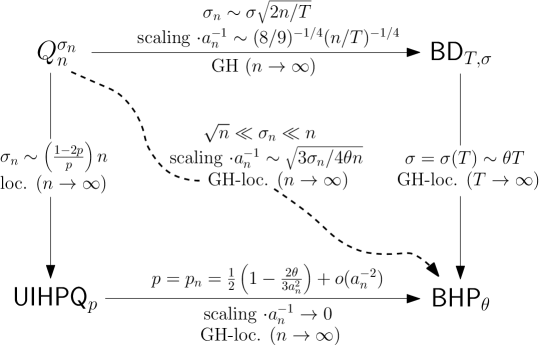
Figure 2: Illustration of various convergences explaining the connections between the spaces $\textup{{UIHPQ}}_{p}$, $\textup{{BHP}}_{\theta}$ and $\textup{{BD}}_{T,\sigma}$. For simplicity, the cases $\theta=0$ and $\theta=\infty$ are left out. The top-most horizontal convergence represents [12, Theorem 1] and holds for $T,\sigma>0$ fixed. If the volume $T$ of $\textup{{BD}}_{T,\sigma}$ is blown up and the perimeter $\sigma$ grows linearly in $T$ such that $\sigma(T)\sim\theta T$, the space $\textup{{BHP}}_{\theta}$ appears as the distributional local Gromov-Hausdorff limit of the disks $\textup{{BD}}_{T,\sigma(T)}$ around their roots ([8, Corollary 3.17]). On the other hand, $\textup{{BHP}}_{\theta}$ is approximated by uniform quadrangulations $Q_{n}^{\sigma_{n}}$ ([8, Theorem 3.4]), or by the $\textup{{UIHPQ}}_{p}$ when $p=p(a_{n},\theta)$ depends in the right way on $\theta$ and $a_{n}$ (Theorem 2). The $\textup{{UIHPQ}}_{p}$ for fixed $p\in[0,1/2]$ in turn arises as the local limit of $Q_{n}^{\sigma_{n}}$, provided the boundary lengths are properly chosen (Theorem 1).

Remark 4.

We stress that the spaces $\textup{{BHP}}_{\theta}$ can also be understood as Gromov-Hausdorff scaling limits of uniform quadrangulations $Q_{n}^{\sigma_{n}}\in\mathcal{Q}_{n}^{\sigma_{n}}$; see [8, Theorems 3.3, 3.4, 3.5]. More specifically, the $\textup{{BHP}}_{\theta}$ for $\theta\in(0,\infty)$ arises when $\sqrt{n}\ll\sigma_{n}\ll n$ and the graph metric is rescaled by a factor $a_{n}^{-1}$ satisfying $3\sigma_{n}a_{n}^{2}/(4n)\rightarrow\theta$ as $n$ tends to infinity. The Brownian half-plane $\textup{{BHP}}_{0}$ corresponding to the choice $\theta=0$ appears more generally when $1\ll\sigma_{n}\ll n$ and $1\ll a_{n}\ll\min\{\sqrt{\sigma_{n}},\sqrt{n/\sigma_{n}}\}$. Finally, the SCRT corresponding to $\theta=\infty$ appears when $\sigma_{n}\gg\sqrt{n}$ and $\max\{1,\,\sqrt{n/\sigma_{n}}\}\ll a_{n}\ll\sqrt{\sigma_{n}}$.

We may as well view the spaces $\textup{{BHP}}_{\theta}$ as local scaling limits around the roots of the so-called Brownian disks $\textup{{BD}}_{T,\sigma}$ of volume $T>0$ and perimeter $\sigma>0$ introduced in [12]. More concretely, it was proved in [8, Corollaries 3.17, 3.18] that when both $T$ and $\sigma=\sigma(T)$ tend to infinity such that $\sigma(T)/T\rightarrow\theta\in[0,\infty]$, then the $\textup{{BHP}}_{\theta}$ is the local Gromov-Hausdorff limit in law of the disk $\textup{{BD}}_{T,\sigma(T)}$ around a boundary point chosen according to the boundary measure of the latter. Figure 2 depicts some convergences involving the families $\textup{{UIHPQ}}_{p}$ and $\textup{{BHP}}_{\theta}$.

2.3 Tree structure

We will prove that for $p<1/2$, the $\textup{{UIHPQ}}_{p}$ can be represented as a collection of independent finite quadrangulations with a simple boundary glued along a tree structure. The tree structure is encoded by the looptree associated to a two-type version of Kesten’s tree, and the finite quadrangulations are distributed according to the Boltzmann distribution $\widehat{\mathbb{P}}^{\sigma}_{g}$ on quadrangulations with a simple boundary of size $2\sigma$. Precise definitions of the encoding objects are postponed to Section 3.

For $0\leq p\leq 1/2$, let $g_{p}=p(1-p)/3$ and $z_{p}=(1-p)/4$. Let $F(g,z)$ be the partition function of the Boltzmann measure on finite rooted quadrangulations with a boundary, with weight $g$ per inner face and $\sqrt{z}$ per boundary edge. Let moreover $\widehat{F}_{k}(g)$ be the partition function of the Boltzmann measure on finite rooted quadrangulations with a simple boundary of perimeter $2k$, with weight $g$ per inner face.

We introduce two probability measures $\mu_{\circ}$ and $\mu_{\bullet}$ on $\mathbb{N}_{0}$ by setting

$$\mu_{\circ}(k) =\frac{1}{F(g_{p},z_{p})}\left(1-\frac{1}{F(g_{p},z_{p})}\right)^{k},\quad k\in\mathbb{N}_{0},$$

$$\mu_{\bullet}(2k+1) =\frac{1}{F(g_{p},z_{p})-1}\left[z_{p}F^{2}(g_{p},z_{p})\right]^{k+1}\widehat{F}_{k+1}(g_{p}),\quad k\in\mathbb{N}_{0},$$

with $\mu_{\bullet}(k)=0$ if $k$ even. Exact expressions for $F(g_{p},z_{p})$ and $\widehat{F}_{k+1}(g_{p})$ are given in (15) and (16) below. The fact that $\mu_{\bullet}$ is a probability distribution is a consequence of Identity (2.8) in [15]. We will prove in Lemma 11 that the pair $(\mu_{\circ},\mu_{\bullet})$ is critical for $0\leq p<1/2$, in the sense that the product of their respective means equals one, and subcritical if $p=1/2$, meaning that the product of their means is strictly less than one. Moreover, both measures have small exponential moments. Our main result characterizing the structure of the $\textup{{UIHPQ}}_{p}$ for $0\leq p<1/2$ is the following.

Theorem 4.

Let $0\leq p<1/2$, and let $\operatorname{\textup{Loop}}(\mathcal{T}_{\infty})$ be the infinite looptree associated to Kesten’s two-type tree $\mathcal{T}_{\infty}(\mu_{\circ},\mu_{\bullet})$. Glue into each inner face of $\operatorname{\textup{Loop}}(\mathcal{T}_{\infty})$ of degree $2\sigma$ an independent Boltzmann quadrangulation with a simple boundary distributed according to $\widehat{\mathbb{P}}^{\sigma}_{g_{p}}$. Then, the resulting infinite quadrangulation is distributed as the $\textup{{UIHPQ}}_{p}$.

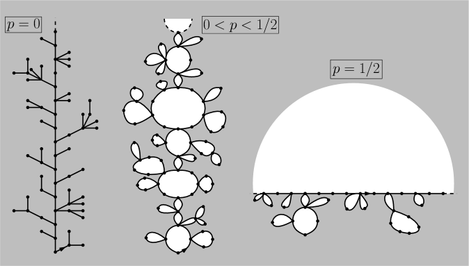
Figure 3: Schematic representation of the $\textup{{UIHPQ}}_{p}$ for $p\in[0,1/2]$. On the left: The $\textup{{UIHPQ}}_{0}$, that is, Kesten’s tree associated to the critical geometric offspring distribution $\mu_{1/2}$. On the right: The standard uniform infinite half-planar quadrangulation UIHPQ with a general boundary. The white parts are understood to be filled in with quadrangulations, the big white semicircle representing the half-plane. In the middle: The $\textup{{UIHPQ}}_{p}$ with skewness parameter $p$. The white parts represent the (finite-size) quadrangulations with a simple boundary which are glued into the loops of the infinite looptree $\operatorname{\textup{Loop}}(\mathcal{T}_{\infty})$ associated to a two-type version $\mathcal{T}_{\infty}(\mu_{\circ},\mu_{\bullet})$ of Kesten’s tree.

The gluing operation fills in each (rooted) loop a finite-size quadrangulation with a simple boundary, which has the same perimeter as the loop. The two boundaries are glued together, such that the root edges of the loop and the quadrangulation get identified; see Remark 8. Figure 3 depicts the above representation of the $\textup{{UIHPQ}}_{p}$ in the case $0<p<1/2$, as well as the borderline cases $p=0$ and $p=1/2$. The branching structure of the standard $\textup{{UIHPQ}}=\textup{{UIHPQ}}_{1/2}$ has been investigated by Curien and Miermont [25]. They show that the UIHPQ can be seen as the uniform infinite half-planar quadrangulation with a simple boundary (represented by the big white semicircle in Figure 3), together with a collection of finite-size quadrangulations with a general boundary, which are attached to the infinite simple boundary.

Remark 5.

In the case $p=0$, the above theorem can be seen as a restatement of Proposition 1. Indeed, in this case, one finds that $\mu_{\circ}=\mu_{1/2}$ is the critical geometric probability law, and $\mu_{\bullet}$ is the Dirac-distribution $\delta_{1}$. By construction, all the inner faces of $\operatorname{\textup{Loop}}(\mathcal{T}_{\infty})$ have then degree $2$, and the gluing of a Boltzmann quadrangulation distributed according to $\widehat{\mathbb{P}}^{1}_{g_{0}=0}$ simply amounts to close the face, by identifying its edges. One finally recovers Kesten’s (one-type) tree associated to the offspring law $\mu_{1/2}$, as already found in Proposition 1.

Remark 6.

In [9], it has been proved that geodesics in the standard UIHPQ intersect both the left and right part of the boundary infinitely many times (see [9, Section 2.3.3] for the exact terminology). However, up to removing finite quadrangulations that hang off from the boundary, the UIHPQ has the topology of a half-plane. Consequently, left and right parts of the boundary intersect only finitely many times. The branching structure described in Theorem 4 implies that the left and right parts of the boundary of the $\textup{{UIHPQ}}_{p}$ for $p<1/2$ have infinitely many intersection points. As a consequence, any infinite self-avoiding path intersects both boundaries infinitely many times.

Our tree-like description of the $\textup{{UIHPQ}}_{p}$ for $0\leq p<1/2$ readily implies that simple random walk on the $\textup{{UIHPQ}}_{p}$ is recurrent. For $p=0$, this result is due to Kesten [31].

Corollary 2.

Let $0\leq p<1/2$. Almost surely, simple random walk on the $\textup{{UIHPQ}}_{p}$ is recurrent.

Somewhat informally, the tree structure describing the $\textup{{UIHPQ}}_{p}$ in the case $p<1/2$ shows that there is an essentially unique way for the random walk to move to infinity. Said otherwise, the walk reduces essentially to a random walk on the half-line reflected at the origin, which is, of course, recurrent. We give a precise proof in terms of electrical networks in Section 6.

Remark 7.

As far as the standard uniform infinite half-planar quadrangulation UIHPQ corresponding to $p=1/2$ is concerned, Angel and Ray [6] prove recurrence of the triangular analog with a simple boundary, the half-plane UIPT. They construct a full-plane extension of the half-plane UIPT using a decomposition into layers and then adapt the methods of Gurel-Gurevich and Nachmias [26], and Benjamini and Schramm [10]. It is believed that the arguments of [6] can be extended to the UIHPQ, too. Ray proves in [38] of recurrence of the half-plane models $\mathbb{H}_{\alpha}$ when $\alpha<2/3$. In [13], Björnberg and Stefánsson prove that the (local) limit of bipartite Boltzmann planar maps is recurrent, for every choice of the weight sequence.

We believe that the mean displacement of a random walker after $n$ steps on the $\textup{{UIHPQ}}_{p}$ for $p<1/2$ is of order $n^{1/3}$, as for Kesten’s tree (case $p=0$). We will not pursue this further in this paper.

Let us finally mention another consequence of Theorem 4 concerning percolation thresholds. See, e.g., [4] for the terminology of Bernoulli percolation on random lattices.

Corollary 3.

Let $0\leq p<1/2$. The critical thresholds for Bernoulli site, bond and face percolation on the $\textup{{UIHPQ}}_{p}$ are almost surely equal to one.

Therefore, percolation on the $\textup{{UIHPQ}}_{p}$ changes drastically depending on whether the skewness parameter $p$ (not to be confused the the percolation parameter) is less or equal to $1/2$: In the standard $\textup{{UIHPQ}}=\textup{{UIHPQ}}_{1/2}$, the critical thresholds are known to be $5/9$ for site percolation, see [39], and $1/3$ for edge percolation and $3/4$ for face percolation, see [4]. The proof of the corollary follows immediately from Theorem 4.

3 Random half-planes and trees

In this section, we begin with a review of the one-parameter family of Brownian half-planes ${\textup{{BHP}}}_{\theta}$, $\theta\geq 0$, introduced in [8] (see also [27] for the case $\theta=0$).

We then gather certain concepts around trees, which play an important role throughout this paper. We properly define the SCRT, two-type Galton-Watson trees and Kesten’s infinite versions thereof, looptrees and the so-called tree of components.

3.1 The Brownian half-planes ${\textup{{BHP}}}_{\theta}$

We need some preliminary notation. Given a function $f=(f_{t},t\in\mathbb{R})$, we set $\underline{f}_{t}=\inf_{[0,t]}f$ for $t\geq 0$ and $\underline{f}_{t}=\inf_{(-\infty,t]}f$ for $t<0$. Moreover, if $f=(f_{t},t\geq 0)$ is a real-valued function indexed by the non-negative reals, its Pitman transform $\pi(f)$ is defined by

$$\pi(f)_{t}=f_{t}-2\underline{f}_{t}.$$

In case $B=(B_{t},t\geq 0)$ is a standard one-dimensional Brownian motion, its Pitman transform $\pi(B)=(\pi(B)_{t},t\geq 0)$ is equal in law to a three-dimensional Bessel process, which has in turn the law of the modulus of a three-dimensional Brownian motion.

Now fix $\theta\in[0,\infty)$. The Brownian half-plane $\textup{{BHP}}_{\theta}$ with skewness $\theta$ is defined in terms of its contour and label processes $X^{\theta}=(X^{\theta}_{t},t\in\mathbb{R})$ and $W^{\theta}=(W^{\theta}_{t},t\in\mathbb{R})$. They are characterized as follows.

• The process $(X^{\theta}_{t},t\geq 0)$ has the law of a one-dimensional Brownian motion $B=(B_{t},t\geq 0)$ with drift $-\theta$ and $B_{0}=0$, and $(X^{\theta}_{-t},t\geq 0)$ has the law of the Pitman transform of an independent copy of $B$.

• Given $X^{\theta}$, the (label) function $W^{\theta}$ has same distribution as $(\gamma_{-\underline{X}_{t}^{\theta}}+Z^{\theta}_{t},t\in\mathbb{R})$, where

  • The process $Z^{\theta}=(Z^{\theta}_{t},t\in\mathbb{R})=Z^{X^{\theta}-\underline{X}^{\theta}}$ is a continuous modification of the centered Gaussian process with conditional covariances given by

    $$\mathbb{E}\left[Z^{\theta}_{s}Z^{\theta}_{t}\,|\,\right]=\min_{[s\wedge t,s\vee t]}X^{\theta}-\underline{X}^{\theta},$$

  • The process $(\gamma_{x},x\in\mathbb{R})$ is a two-sided Brownian motion with $\gamma_{0}=0$ and scaled by the factor $\sqrt{3}$, independent of $Z^{\theta}$.

The process $Z^{\theta}$ is usually called the (head of the) random snake driven by $X^{\theta}-\underline{X}^{\theta}$, see [33] for more on this. Next, we define two pseudo-metrics $d_{X^{\theta}}$ and $d_{W^{\theta}}$ on $\mathbb{R}$,

$$d_{X^{\theta}}(s,t)=X^{\theta}_{s}+X^{\theta}_{t}-2\min_{[s\wedge t,s\vee t]}X^{\theta},\quad\textup{and}\quad d_{W^{\theta}}(s,t)=W^{\theta}_{s}+W^{\theta}_{t}-2\min_{[s\wedge t,s\vee t]}W^{\theta}.$$

The pseudo-metric $D_{\theta}$ associated to $\textup{{BHP}}_{\theta}$ is defined as the maximal pseudo-metric $d$ on $\mathbb{R}$ satisfying $d\leq d_{W^{\theta}}$ and $\{d_{X^{\theta}}=0\}\subseteq\{D_{\theta}=0\}$. According to Chapter $3$ of [18], it admits the expression ($s,t\in\mathbb{R}$)

$$D_{\theta}(s,t)=\inf\left\{\sum_{i=1}^{k}d_{W^{\theta}}(s_{i},t_{i}):\begin{array}[]{l}k\in\mathbb{N},\,s_{1},\ldots,s_{k},t_{1},\ldots,t_{k}\in\mathbb{R},s_{1}=s,t_{k}=t,\\ d_{X^{\theta}}(t_{i},s_{i+1})=0\mbox{ for every }i\in\{1,\ldots,k-1\}\end{array}\right\}\,.$$

Definition 1.

The Brownian half-plane $\textup{{BHP}}_{\theta}$ has the law of the pointed metric space $(\mathbb{R}/\{D_{\theta}=0\},D_{\theta},\rho_{\theta})$, with the distinguished point $\rho_{\theta}$ is given by the equivalence class of $0$.

Note that $D_{\theta}$ stands here also for the induced metric on the quotient space. It follows from standard scaling properties of $X^{\theta}$ and $W^{\theta}$ that for $\lambda>0$, $\lambda\cdot\textup{{BHP}}_{\theta}=_{d}\textup{{BHP}}_{\theta/\lambda^{2}}$. In particular, $\textup{{BHP}}_{0}$ is scale-invariant. It was shown in [8] that for every $\theta\geq 0$, $\textup{{BHP}}_{\theta}$ has a.s. the topology of the closed half-plane $\overline{\mathbb{H}}=\mathbb{R}\times\mathbb{R}_{+}$.

3.2 Random trees and some of their properties

3.2.1 The self-similar continuum random tree SCRT

Introduced by Aldous in [2], the SCRT is a random rooted real tree that forms the non-compact analog of the usual continuum random tree CRT. Consider the stochastic process $(X_{t},t\in\mathbb{R})$ such that $(X_{t},t\geq 0)$ and $(X_{-t},t\geq 0)$ are two independent one-dimensional standard Brownian motions started at zero. Define on $\mathbb{R}$ the pseudo-metric

$$d_{X}(s,t)=X_{s}+X_{t}-2\min_{[s\wedge t,s\vee t]}X.$$

Definition 2.

The SCRT is the continuum random real tree $\mathcal{T}_{X}$ coded by $X$, i.e., the SCRT has the law of the pointed metric space $(\mathcal{T}_{X},d_{X},[0])$, where $\mathcal{T}_{X}=\mathbb{R}/\{d_{X}=0\}$, and the distinguished point is given by the equivalence class of $0$.

The SCRT is self-similar, meaning that $\lambda\cdot\textup{{SCRT}}=_{d}\textup{{SCRT}}$ for $\lambda>0$, and invariant under re-rooting. We remark that the SCRT is often defined in terms of two independent three-dimensional Bessel processes $(X_{t},t\geq 0)$ and $(X_{-t},t\geq 0)$. Since the Pitman transform $\pi$ turns a Brownian motion into a three-dimension Bessel processes, it is readily seen that both definitions give rise to the same random tree.

3.2.2 Galton-Watson trees

We recall the formalism of (finite or infinite) plane trees, i.e., rooted ordered trees. The size $|\mathsf{t}|\in\mathbb{N}_{0}\cup\{\infty\}$ of $\mathsf{t}$ is given by its number of edges, and we shall write $\mathbb{T}_{f}$ for the set of all finite plane trees.

We will often use the fact that if $\mathsf{GW}_{\nu}$ denotes the law of a Galton-Watson tree with critical or subcritical offspring distribution $\nu$, then

$$\mathsf{GW}_{\nu}(\mathsf{t})=\prod_{u\in V(\mathsf{t})}\nu(k_{u}(\mathsf{t})),\quad t\in\mathbb{T}_{f},$$ (1)

where for $u\in V(\mathsf{t})$, $k_{u}(\mathsf{t})$ is the number of offspring of vertex $u$. See, for example, [34, Proposition 1.4]). In the case where $\nu=\mu_{p}$ is the geometric offspring distribution of parameter $1-p$ with $p\in[0,1/2]$, (1) becomes

$$\mathsf{GW}_{\mu_{p}}(\mathsf{t})=p^{|\mathsf{t}|}(1-p)^{|\mathsf{t}|+1}.$$ (2)

From the last display, the connection to random walks is apparent. Namely, let $(S^{(p)}(m),m\in\mathbb{N}_{0})$ be a random walk on the integers starting from $S^{(p)}(0)=0$ with increments distributed according to $p\delta_{1}+(1-p)\delta_{-1}$. Define the first hitting time of $-1$,

$$T_{-1}^{(p)}=\inf\{m\in\mathbb{N}:S^{(p)}(m)=-1\}.$$

Then it is readily deduced from (2) that the size $|\mathsf{t}|$ of $\mathsf{t}$ under $\mathsf{GW}_{\mu_{p}}$ and $(T^{(p)}_{-1}-1)/2$ are equal in distribution. To be precise, by Kemperman’s formula [37, Section 6.1], we have

$$\mathbb{P}\left(T_{-1}^{(p)}=2n+1\right)=\frac{1}{2n+1}\mathbb{P}\left(S^{(p)}_{2n+1}=-1\right)=\frac{1}{2n+1}{2n+1\choose n+1}p^{n}(1-p)^{n+1},\quad n\in\mathbb{N}_{0},$$

and the $n$th Catalan number $\tfrac{1}{n+1}{2n\choose n}$ is precisely the number of plane trees with $n$ edges.

Given a finite or infinite plane tree, it will be convenient to say that vertices at even height of $\mathsf{t}$ are white, and those at odd height are black. We use the notation $V(\mathsf{t}_{\circ})$ and $V(\mathsf{t}_{\bullet})$ for the associated subsets of vertices. We next define two-type Galton-Watson trees associated to a pair $(\nu_{\circ},\nu_{\bullet})$ of probability measures on $\mathbb{N}_{0}$.

Definition 3.

The two-type Galton-Watson tree with a pair of offspring distributions $(\nu_{\circ},\nu_{\bullet})$ is the random plane tree such that vertices at even height have offspring distribution $\nu_{\circ}$, vertices at odd height have offspring distribution $\nu_{\bullet}$, and the numbers of children of the different vertices are independent.

In this context, the pair $(\nu_{\circ},\nu_{\bullet})$ is said to be critical if and only if the mean vector $(m_{\circ},m_{\bullet})$ satisfies $m_{\circ}m_{\bullet}=1$. Then, the law $\mathsf{GW}_{\nu_{\circ},\nu_{\bullet}}$ of such a tree is characterized by

$$\mathsf{GW}_{\nu_{\circ},\nu_{\bullet}}(\mathsf{t})=\prod_{u\in V(\mathsf{t}_{\circ})}\nu_{\circ}(k_{u}(\mathsf{t}))\prod_{u\in V(\mathsf{t}_{\bullet})}\nu_{\bullet}(k_{u}(\mathsf{t})),\quad t\in\mathbb{T}_{f}.$$

3.2.3 Kesten’s tree and its two-type version

We next briefly review critical Galton-Watson trees conditioned to survive; see [31] or [36], and [40] for the multi-type case.

Proposition 3 (Theorem 3.1 in [40]).

Let $\mathsf{GW}$ be the law of a critical (either one or two-type) Galton-Watson tree. For every $n\in\mathbb{N}$, assume that $\mathsf{GW}(\{\#V(\mathsf{t})=n\})>0$, and let $\mathcal{T}_{n}$ be a tree with law $\mathsf{GW}$ conditioned to have $n$ vertices. Then, we have the local convergence for the metric $d_{\textup{map}}$ as $n\rightarrow\infty$ to a random infinite tree $\mathcal{T}_{\infty}$,

$$\mathcal{T}_{n}\overset{(d)}{\longrightarrow}\mathcal{T}_{\infty}.$$

In the case $\mathsf{GW}=\mathsf{GW}_{\nu}$ for $\nu$ a critical one-type offspring distribution, $\mathcal{T}_{\infty}$ is often called Kesten’s tree associated to $\nu$, and simply Kesten’s tree if $\nu=\mu_{1/2}$. We will use the same terminology if $(\nu_{\circ},\nu_{\bullet})$ is a critical pair of offspring distributions and $\mathsf{GW}=\mathsf{GW}_{\nu_{\circ},\nu_{\bullet}}$. In this case, we write $\mathcal{T}_{\infty}(\nu_{\circ},\nu_{\bullet})$ for Kesten’s tree associated to $(\nu_{\circ},\nu_{\bullet})$. Note that the condition $\mathsf{GW}(\{\#V(\mathsf{t})=n\})>0$ can be relaxed, provided we can find a subsequence along which this condition is satisfied.

Galton-Watson trees conditioned to survive enjoy an explicit construction, which we briefly recall for the two-type case. Details can be found in [40]. Let $(\nu_{\circ},\nu_{\bullet})$ be a critical pair of offspring distributions with mean $(m_{\circ},m_{\bullet})$, and recall that the size-biased distributions $\bar{\nu}_{\circ}$ and $\bar{\nu}_{\bullet}$ are defined by

$$\bar{\nu}_{\circ}(k)=\frac{k\nu_{\circ}(k)}{m_{\circ}}\quad\text{and}\quad\bar{\nu}_{\bullet}(k)=\frac{k\nu_{\bullet}(k)}{m_{\bullet}},\quad k\in\mathbb{N}_{0}.$$

Kesten’s tree $\mathcal{T}_{\infty}$ associated to $(\nu_{\circ},\nu_{\bullet})$ is an infinite locally finite (two-type) tree that has a.s. a unique infinite self-avoiding path called the spine. It is constructed as follows. The root vertex (white) is the first vertex on the spine. It has offspring distribution $\bar{\nu}_{\circ}$. Among its offspring, a child (black) is chosen uniformly at random to be the second vertex on the spine. It has offspring distribution $\bar{\nu}_{\bullet}$, and a child (white) chosen uniformly at random among its offspring becomes the third vertex on the spine. The spine is constructed by iterating this procedure.

The construction of the tree is completed by specifying that vertices at even (resp. odd) height lying not on the spine have offspring distribution $\nu_{\circ}$ (resp. $\nu_{\bullet}$), and that the numbers of offspring of the different vertices are independent.

The construction is similar in the mono-type case. In the particular case when $\nu=\mu_{1/2}$ is the geometric distribution with parameter $1/2$, Kesten’s tree can be represented by an infinite half-line (isomorphic to $\mathbb{N}$) and a collection of independent Galton-Watson trees with law $\mathsf{GW}_{\mu_{1/2}}$ grafted to the left and to the right of every vertex on the spine; see, for instance, [29, Example 10.1]. We will exploit this representation in our proof of Proposition 1.

3.2.4 Random looptrees

Our description of the $\textup{{UIHPQ}}_{p}$ in Theorem 4 makes use of so-called looptrees, which were introduced in [22]. A looptree can informally be seen as a collection of loops glued along a tree structure. The following presentation is inspired by [23, Section 2.3]. We use, however, slightly different definitions which are better suited to our purpose. In particular, given a plane tree $\mathsf{t}$, we will only replace vertices $v\in V(\mathsf{t}_{\bullet})$ at odd height by loops of length $\deg(u)$. Consequently, several loops may be attached to one and the same vertex (at even height).

Let us now make things more precise. Let $\mathsf{t}$ be a finite plane tree, and recall that vertices at even height are white, and those at odd height are black (with respective subsets of vertices $V(\mathsf{t}_{\circ})$ and $V(\mathsf{t}_{\bullet})$). We associate to $\mathsf{t}$ a rooted looptree $\operatorname{\textup{Loop}}(\mathsf{t})$ as follows. Around every (black) vertex in $V(\mathsf{t}_{\bullet})$, we connect its incident white vertices in cyclic order, so that they form a loop. Then $\operatorname{\textup{Loop}}(\mathsf{t})$ is the planar map obtained from erasing the black vertices and the edges of $\mathsf{t}$. We root $\operatorname{\textup{Loop}}(\mathsf{t})$ at the edge connecting the origin of $\mathsf{t}$ to the last child of its first sibling in $\mathsf{t}$; see Figure 4.

The reverse application associates to a looptree $\mathsf{l}$ a plane tree, which we call the tree of components $\operatorname{\textup{Tree}}(\mathsf{l})$. In order to obtain $\operatorname{\textup{Tree}}(\mathsf{l})$ from $\mathsf{l}$, we add a new vertex in every internal face of $\mathsf{l}$ and connect this vertex to all the vertices of the face. The root edge of $\operatorname{\textup{Tree}}(\mathsf{l})$ connects the origin of $\mathsf{l}$ to the new vertex added in the face incident to the left side of the root edge of $\mathsf{l}$.

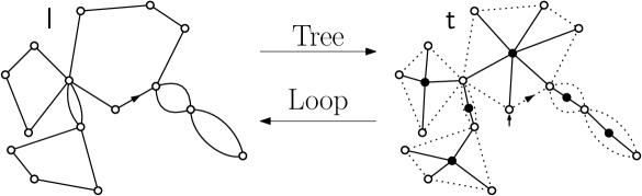
Figure 4: A looptree and the associated tree of components.

The procedures $\operatorname{\textup{Tree}}$ and $\operatorname{\textup{Loop}}$ extend to infinite but locally finite trees, by considering the consistent sequence of maps $\{\operatorname{\textup{Loop}}(\textup{Ball}_{2k}(\mathsf{t})):k\in\mathbb{N}_{0}\}$. We will be interested in the random infinite looptree associated to Kesten’s two-type tree.

Definition 4.

If $(\nu_{\circ},\nu_{\bullet})$ is a critical pair of offspring laws and $\mathcal{T}_{\infty}$ the corresponding Kesten’s tree, we call the random infinite looptree $\operatorname{\textup{Loop}}(\mathcal{T}_{\infty})$ Kesten’s looptree associated to $\mathcal{T}_{\infty}$.

Note that a formal way to construct $\operatorname{\textup{Loop}}(\mathcal{T}_{\infty})$ is to define it as the local limit of $\operatorname{\textup{Loop}}(\mathcal{T}_{n})$, where $\mathcal{T}_{n}$ is a two-type Galton-Watson tree with offspring distribution $(\nu_{\circ},\nu_{\bullet})$ conditioned to have $n$ vertices.

Remark 8.

In a looptree $\mathsf{l}$, every loop is naturally rooted at the edge whose origin is the closest vertex to the origin of $\mathsf{l}$, such that the outer face of $\mathsf{l}$ lies to the right of that edge. The gluing of a (rooted) quadrangulation with a simple boundary of perimeter $2\sigma$ into a loop of the same length is then determined by the convention that the root edge of the quadrangulation is glued on the root edge of the loop.

4 Construction of the ${\textup{{UIHPQ}}}_{p}$

A Schaeffer-type bijection due to Bouttier, Di Francesco and Guitter [14] encodes quadrangulations with a boundary in terms of labeled trees that are attached to a bridge. We shall first describe a bijective encoding of finite-size planar quadrangulations, and then extend it to infinite quadrangulations with an infinite boundary. This will allow us to construct and define the $\textup{{UIHPQ}}_{p}$ for $p\in[0,1/2]$ in terms of the encoding objects, which we define first.

4.1 The encoding objects

We briefly review well-labeled trees, forests, bridges and contour and label functions. Our notation bears similarities to [25, 19, 8], differs, however, at some places. Each of these references already contains the construction of the standard UIHPQ.

4.1.1 Forest and bridges

A well-labeled tree $(\mathsf{t},\ell)$ is a pair consisting of a finite rooted plane tree $\mathsf{t}$ and a labeling $(\ell(u))_{u\in V(\mathsf{t})}$ of its vertices $V(\mathsf{t})$ by integers, with the constraints that the root vertex receives label zero, and $|\ell(u)-\ell(v)|\leq 1$ if $u$ and $v$ are connected by an edge.

A well-labeled forest with $\sigma\in\mathbb{N}$ trees is a pair $(\textup{$\mathfrak{f}$},\textup{$\mathfrak{l}$})$, where $\textup{$\mathfrak{f}$}=(\mathsf{t}_{0},\ldots,\mathsf{t}_{\sigma-1})$ is a sequence of $\sigma$ rooted plane trees, and $\textup{$\mathfrak{l}$}:V(\textup{$\mathfrak{f}$})\rightarrow\mathbb{Z}$ is a labeling of the vertices $V(\textup{$\mathfrak{f}$})=\cup_{i=0}^{\sigma-1}V(\mathsf{t}_{i})$ such that for every $0\leq i\leq\sigma-1$, the pair $(\mathsf{t}_{i},\textup{$\mathfrak{l}$}\restriction V(\mathsf{t}_{i}))$ is a well-labeled tree. Similarly, a well-labeled infinite forest is a pair $(\textup{$\mathfrak{f}$},\textup{$\mathfrak{l}$})$, where $\textup{$\mathfrak{f}$}=(\mathsf{t}_{i},i\in\mathbb{Z})$ is an infinite collection of rooted plane trees, together with a labeling $\textup{$\mathfrak{l}$}:\cup_{i\in\mathbb{Z}}V(\mathsf{t}_{i})\rightarrow\mathbb{Z}$ such that for each $i\in\mathbb{Z}$, the restriction of $\mathfrak{l}$ to $V(\mathsf{t}_{i})$ turns $\mathsf{t}_{i}$ into a well-labeled tree.

A bridge of length $2\sigma$ for $\sigma\in\mathbb{N}$ is a sequence $\textup{{b}}=(\textup{{b}}(0),\textup{{b}}(1),\ldots,\textup{{b}}(2\sigma-1))$ of $2\sigma$ integers with $\textup{{b}}(0)=0$ and $|\textup{{b}}(i+1)-\textup{{b}}(i)|=1$ for $0\leq i\leq 2\sigma-1$, where we agree that $\textup{{b}}(2\sigma)=0$. In a similar manner, an infinite bridge is a two-sided sequence $\textup{{b}}=(\textup{{b}}(i):i\in\mathbb{Z})$ with $\textup{{b}}(0)=0$ and $|\textup{{b}}(i+1)-\textup{{b}}(i)|=1$ for all $i\in\mathbb{Z}$.

Given a bridge b, an index $i$ for which $\textup{{b}}(i+1)=\textup{{b}}(i)-1$ is called a down-step of b. The set of all down-steps of b is denoted $\textup{{DS}}(\textup{{b}})$. If b is a bridge of length $2\sigma$, $\textup{{DS}}(\textup{{b}})$ has $\sigma$ elements, and we write $\textup{d}^{\downarrow}_{\textup{{b}}}(i)$ for the $i$th smallest element in $\textup{{DS}}(\textup{{b}})$, for $i=1,\ldots,\sigma$. If b is an infinite bridge and $i\in\mathbb{N}$, $\textup{d}^{\downarrow}_{\textup{{b}}}(i)$ denotes the $i$th smallest element in $\textup{{DS}}(\textup{{b}})\cap\mathbb{N}_{0}$, and $\textup{d}^{\downarrow}_{\textup{{b}}}(-i)$ denotes the $i$th largest element in $\textup{{DS}}(\textup{{b}})\cap\mathbb{Z}_{<0}$. If there is no danger of confusion, we write simply $\textup{d}^{\downarrow}$ instead of $\textup{d}^{\downarrow}_{\textup{{b}}}$.

The size of a forest $\mathfrak{f}$ is the number $|\textup{$\mathfrak{f}$}|\in\mathbb{N}_{0}\cup\{\infty\}$ of tree edges. If $\textup{$\mathfrak{f}$}=(\mathsf{t}_{0},\dots,\mathsf{t}_{\sigma-1})$ and $u\in V(\mathsf{t}_{i})$, we write $\textup{H}_{\textup{$\mathfrak{f}$}}(u)$ for the height of $u$ in the tree $\mathsf{t}_{i}$, i.e., the graph distance to the root of $\mathsf{t}_{i}$. Moreover, $\mathcal{I}_{\textup{$\mathfrak{f}$}}(u)=i$ denotes the index of the tree the vertex $u$ belongs to. Both $\textup{H}_{\textup{$\mathfrak{f}$}}$ and $\mathcal{I}_{\textup{$\mathfrak{f}$}}$ extend in the obvious way to infinite forests. If it is clear which forest we are referring to, we drop the subscript $\mathfrak{f}$ in H and $\mathcal{I}$.

We let $\textup{$\mathfrak{F}$}_{\sigma}^{n}=\{(\textup{$\mathfrak{f}$},\textup{$\mathfrak{l}$}):\textup{$\mathfrak{f}$}\textup{ has }\sigma\textup{ trees and size }|\textup{$\mathfrak{f}$}|=n\}$ be the set of all well-labeled forests of size $n$ with $\sigma$ trees and write $\textup{$\mathfrak{F}$}_{\infty}$ for the set of all well-labeled infinite forests. The set of all bridges of length $2\sigma$ is denoted $\textup{$\mathfrak{B}$}_{\sigma}$. As far as infinite bridges are concerned, it will be sufficient to consider only those bridges b which satisfy $\inf_{i\in\mathbb{N}}\textup{{b}}(i)=-\infty$ and $\inf_{i\in\mathbb{N}}\textup{{b}}(-i)=-\infty$, and we denote the set of them by $\textup{$\mathfrak{B}$}_{\infty}$.

4.1.2 Contour and label function

We first consider the case $((\textup{$\mathfrak{f}$},\textup{$\mathfrak{l}$}),\textup{{b}})\in\textup{$\mathfrak{F}$}_{\sigma}^{n}\times\textup{$\mathfrak{B}$}_{\sigma}$ for some $n,\sigma\in\mathbb{N}$. By a slight abuse of notation, we write $\textup{$\mathfrak{f}$}(0),\ldots,\textup{$\mathfrak{f}$}(2n+\sigma-1)$ for the contour exploration of $\mathfrak{f}$, that is, the sequence of vertices (with multiplicity) which we obtain from walking around the trees $\mathsf{t}_{0},\ldots,\mathsf{t}_{\sigma-1}$ of $\mathfrak{f}$, one after the other in the contour order. See the left side of Figure 5. We define the contour function of $(\textup{$\mathfrak{f}$},\textup{$\mathfrak{l}$})$ by

$$C_{\textup{$\mathfrak{f}$}}(j)=\textup{H}(\textup{$\mathfrak{f}$}(j))-\mathcal{I}(\textup{$\mathfrak{f}$}(j)),\quad 0\leq j\leq 2n+\sigma-1.$$

Note that $C_{\textup{$\mathfrak{f}$}}(2n+\sigma-1)=-\sigma-1$, since the last visited vertex by the contour exploration is the root of $\mathsf{t}_{\sigma-1}$. We extend $C_{\textup{$\mathfrak{f}$}}$ to $[0,2n+\sigma]$ by first letting $C_{\textup{$\mathfrak{f}$}}(2n+\sigma)=-\sigma$, and then by linear interpolation between integers, so that $C_{\textup{$\mathfrak{f}$}}$ becomes a continuous real-valued function on $[0,2n+\sigma]$ starting at zero and ending at $-\sigma$.

The label function associated to $((\textup{$\mathfrak{f}$},\textup{$\mathfrak{l}$}),\textup{{b}})$ is obtained from shifting the vertex label $\textup{$\mathfrak{l}$}(\textup{$\mathfrak{f}$}(j))$ by the value of the bridge b evaluated at its $(\mathcal{I}(\textup{$\mathfrak{f}$}(j))+1)$th down-step. Formally,

$$\textup{$\mathfrak{L}$}_{\textup{$\mathfrak{f}$}}(j)=\textup{$\mathfrak{l}$}(\textup{$\mathfrak{f}$}(j))+\textup{{b}}\left(\textup{d}^{\downarrow}\left(\mathcal{I}(\textup{$\mathfrak{f}$}(j))+1\right)\right),\quad 0\leq j\leq 2n+\sigma-1.$$

We let $\textup{$\mathfrak{L}$}_{\textup{$\mathfrak{f}$}}(2n+\sigma)=0$ and again linearly interpolate between integer values, so that $\textup{$\mathfrak{L}$}_{\textup{$\mathfrak{f}$}}$ becomes an element of $\mathcal{C}([0,2n+\sigma],\mathbb{R})$. Contour and label functions are depicted on the right side of Figure 5.

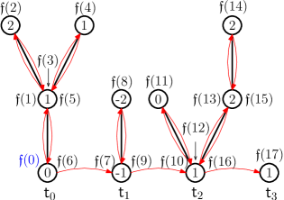
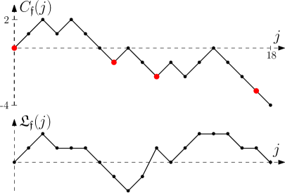
Figure 5: Contour and label functions $C_{\textup{$\mathfrak{f}$}}$ and $\textup{$\mathfrak{L}$}_{\textup{$\mathfrak{f}$}}$ of an element $((\textup{$\mathfrak{f}$},\textup{$\mathfrak{l}$}),\textup{{b}})\in\textup{$\mathfrak{F}$}_{4}^{7}\times\textup{$\mathfrak{B}$}_{4}$. The left side depicts the contour exploration of $\mathfrak{f}$. The labels on the vertices are given by $\textup{$\mathfrak{L}$}_{\textup{$\mathfrak{f}$}}(j)$, $j=0,\ldots,18$. Note that the values of b at its four down-steps are equal to the values of $\textup{$\mathfrak{L}$}_{\textup{$\mathfrak{f}$}}$ at the tree roots: In this example, we have $\textup{{b}}(\textup{d}^{\downarrow}(1))=0$, $\textup{{b}}(\textup{d}^{\downarrow}(2))=-1$, and $\textup{{b}}(\textup{d}^{\downarrow}(3))=\textup{{b}}(\textup{d}^{\downarrow}(4))=1$. The red dots on the right indicate the encoding of a new tree.

In the case $((\textup{$\mathfrak{f}$},\textup{$\mathfrak{l}$}),\textup{{b}})\in\textup{$\mathfrak{F}$}_{\infty}\times\textup{$\mathfrak{B}$}_{\infty}$, we explore the trees of $\mathfrak{f}$ in the following way: First, $(\textup{$\mathfrak{f}$}(0),\textup{$\mathfrak{f}$}(1),\ldots)$ is the sequence of vertices of the contour paths of the trees $\mathsf{t}_{i},i\in\mathbb{N}_{0}$, in the left-to-right order, starting from the root of $\mathsf{t}_{0}$. Then, we let $(\textup{$\mathfrak{f}$}(-1),\textup{$\mathfrak{f}$}(-2),\ldots)$ be the sequence of vertices of the contour paths $\mathsf{t}_{-1},\mathsf{t}_{-2},\ldots$, in the counterclockwise or right-to-left order, starting from the root of $\mathsf{t}_{-1}$; see the left side of Figure 6.

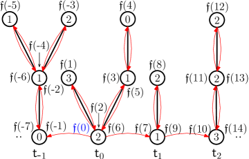
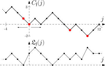
Figure 6: Contour and label functions $C_{\textup{$\mathfrak{f}$}}$ and $\textup{$\mathfrak{L}$}_{\textup{$\mathfrak{f}$}}$ of an element $((\textup{$\mathfrak{f}$},\textup{$\mathfrak{l}$}),\textup{{b}})\in\textup{$\mathfrak{F}$}_{\infty}\times\textup{$\mathfrak{B}$}_{\infty}$. The left side depicts the two-sided contour exploration of $\mathfrak{f}$. The labels are given by $\textup{$\mathfrak{L}$}_{\textup{$\mathfrak{f}$}}(j)$, where now $j\in\mathbb{Z}$. The values of the infinite bridge b at its first three down-steps to the right of $0$ read here $\textup{{b}}(\textup{d}^{\downarrow}(1))=2$, $\textup{{b}}(\textup{d}^{\downarrow}(2))=1$ and $\textup{{b}}(\textup{d}^{\downarrow}(3))=3$, while the first down-step to the left of zero has value $\textup{{b}}(\textup{d}^{\downarrow}(-1))=0$. The arrows below the contour function indicate the direction of the encoding, and the red dots mark again the encoding of a new tree.

Contour and label functions $C_{\textup{$\mathfrak{f}$}}$ and $\textup{$\mathfrak{L}$}_{\textup{$\mathfrak{f}$}}$ are defined similarly to the finite case, namely

$$C_{\textup{$\mathfrak{f}$}}(j) =\textup{H}(\textup{$\mathfrak{f}$}(j))-\mathcal{I}(\textup{$\mathfrak{f}$}(j)),\quad j\in\mathbb{Z},$$

$$\textup{$\mathfrak{L}$}_{\textup{$\mathfrak{f}$}}(j) =\textup{$\mathfrak{l}$}(\textup{$\mathfrak{f}$}(j))+\textup{{b}}\left(\textup{d}^{\downarrow}\left(\mathcal{I}(\textup{$\mathfrak{f}$}(j))+1\right)\right),\quad j\in\mathbb{Z}_{\geq 0},$$

$$\textup{$\mathfrak{L}$}_{\textup{$\mathfrak{f}$}}(j) =\textup{$\mathfrak{l}$}(\textup{$\mathfrak{f}$}(j))+\textup{{b}}\left(\textup{d}^{\downarrow}\left(\mathcal{I}(\textup{$\mathfrak{f}$}(j))\right)\right),\quad j\in\mathbb{Z}_{<0}.$$

Note that the asymmetry in the definition of $\textup{$\mathfrak{L}$}_{\textup{$\mathfrak{f}$}}$ stems from the numbering of the trees. By linear interpolation between integer values, we interpret $C_{\textup{$\mathfrak{f}$}}$, $\textup{$\mathfrak{L}$}_{\textup{$\mathfrak{f}$}}$, and sometimes also $\mathfrak{l}$, as continuous functions (from $\mathbb{R}$ to $\mathbb{R}$).

4.2 The Bouttier-Di Francesco-Guitter mapping

We denote the set of all rooted pointed quadrangulations with $n$ inner faces and $2\sigma$ boundary edges by

$$\mathcal{Q}_{n}^{\sigma,\bullet}=\left\{(\textup{$\mathsf{q}$},v^{\bullet}):\textup{$\mathsf{q}$}\in\mathcal{Q}_{n}^{\sigma},v^{\bullet}\in V(\textup{$\mathsf{q}$})\right\},$$

where $v^{\bullet}$ stands for the distinguished pointed vertex. In the following part, we briefly recall the definition of the bijection $\Phi_{n}:\textup{$\mathfrak{F}$}_{\sigma}^{n}\times\textup{$\mathfrak{B}$}_{\sigma}\rightarrow\mathcal{Q}_{n}^{\sigma,\bullet}$ introduced in [14].

4.2.1 The encoding of finite quadrangulations

We represent an element $((\textup{$\mathfrak{f}$},\textup{$\mathfrak{l}$}),\textup{{b}})\in\textup{$\mathfrak{F}$}_{\sigma}^{n}\times\textup{$\mathfrak{B}$}_{\sigma}$ in the plane as follows. Firstly, we view b as a labeled cycle of length $2\sigma$: We start from a distinguished vertex labeled $\textup{{b}}(0)=0$ and label the remaining $2\sigma-1$ vertices in the counterclockwise order by the values $\textup{{b}}(1),\textup{{b}}(2),\ldots,\textup{{b}}(2\sigma-1)$. Then we graft the trees $(\mathsf{t}_{0},\dots,\mathsf{t}_{\sigma-1})$ of $\mathfrak{f}$ to the $\sigma$ down-steps $0\leq i_{0}<i_{1}<\dots<i_{\sigma-1}\leq 2\sigma-1$ of b, such that $\mathsf{t}_{j}$ is grafted on the vertex corresponding to the value $\textup{{b}}(i_{j})$, in the interior of the cycle. We do it in such a way that different trees do not intersect. The vertices of $\mathsf{t}_{j}$ are equipped with their labels shifted by $\textup{{b}}(i_{j})$. Figure 7 illustrates this procedure.

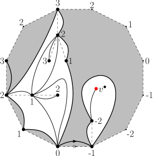
Figure 7: A representation of an element $((\textup{$\mathfrak{f}$},\textup{$\mathfrak{l}$}),\textup{{b}})\in\textup{$\mathfrak{F}$}_{6}^{6}\times\textup{$\mathfrak{B}$}_{6}$ in the plane and the associated rooted pointed quadrangulation $(\textup{$\mathsf{q}$},v^{\bullet})=\Phi_{n}((\textup{$\mathfrak{f}$},\textup{$\mathfrak{l}$}),\textup{{b}})$. The distinguished vertex of the cycle is the down-most vertex labeled $0$. The trees are grafted to the $6$ down-steps of b (here, $\textup{d}^{\downarrow}(1)=0$, $\textup{d}^{\downarrow}(2)=1$, $\textup{d}^{\downarrow}(3)=7$, $\textup{d}^{\downarrow}(4)=9$, $\textup{d}^{\downarrow}(5)=10$, and $\textup{d}^{\downarrow}(6)=11$). The tree edges are indicated by the dashed lines in the interior of the cycle. Note that three trees (those above the first, fourth and sixth down-step) consist of a single vertex. The labels in a tree are shifted by the bridge value of the down-step above which the tree is attached. Note that the 12 boundary edges of the cycle are in a order-preserving correspondence with the 12 boundary edges of $\mathsf{q}$. (The two edges of $\mathsf{q}$ which lie entirely in the outer face are counted twice.)

We now build a rooted and pointed quadrangulation $(\textup{$\mathsf{q}$},v^{\bullet})$ out of $((\textup{$\mathfrak{f}$},\textup{$\mathfrak{l}$}),\textup{{b}})$. First, we put an extra vertex $v^{\bullet}$ in the interior of the cycle representing b. The set of vertices of $\mathsf{q}$ is given by the tree vertices $V(\textup{$\mathfrak{f}$})\cup\{v^{\bullet}\}$. As for the edges of $\mathsf{q}$, we define for $0\leq i\leq 2n+\sigma-1$ the successor $\textup{succ}(i)\in[0,2n+\sigma-1]\cup\{\infty\}$ of $i$ to be the first element $k$ in the list $(i+1,\ldots,2n+\sigma-1,0,\ldots,i-1)$ (from left to right) which has label $\textup{$\mathfrak{L}$}_{\textup{$\mathfrak{f}$}}(k)=\textup{$\mathfrak{L}$}_{\textup{$\mathfrak{f}$}}(i)-1$. If there is no such element, we put $\textup{succ}(i)=\infty$. We extend the contour exploration $\textup{$\mathfrak{f}$}(0),\ldots,\textup{$\mathfrak{f}$}(2n+\sigma-1)$ of $\mathfrak{f}$ by setting $\textup{$\mathfrak{f}$}(\infty)=v^{\bullet}$. We follow the exploration starting from the vertex $\textup{$\mathfrak{f}$}(0)$ (which is the root of $\mathsf{t}_{0}$) and draw for each $0\leq i\leq 2n+\sigma-1$ an arc between $\textup{$\mathfrak{f}$}(i)$ and $\textup{$\mathfrak{f}$}(\textup{succ}(i))$, such that arcs do not cross. Except for the leaves, a vertex of $\mathfrak{f}$ is visited at least twice in the contour exploration, so that there are in general several arcs connecting the vertices $\textup{$\mathfrak{f}$}(i)$ and $\textup{$\mathfrak{f}$}(\textup{succ}(i))$. The edges of $\mathsf{q}$ are given by all these arcs between the vertices $V(\textup{$\mathfrak{f}$})\cup\{v^{\bullet}\}$.

It only remains to root the quadrangulation. To that aim, we observe from Figure 7 that the $2\sigma$ boundary edges of $\mathsf{q}$ are in a order-preserving correspondence with the $2\sigma$ cycle edges. We root $\mathsf{q}$ at the edge corresponding to the first edge of the cycle (starting from the distinguished edge, in the clockwise order), oriented in such a way that the face of degree $2\sigma$ becomes the outer face (i.e., lies to the right of the root edge). Upon erasing the tree and cycle edges of the representation of $((\textup{$\mathfrak{f}$},\textup{$\mathfrak{l}$}),\textup{{b}})$, and the vertices of b corresponding to up-steps, we obtain a rooted pointed quadrangulation $(\textup{$\mathsf{q}$},v^{\bullet})$. A description of the reverse mapping $\Phi_{n}^{-1}:\mathcal{Q}_{n}^{\sigma,\bullet}\rightarrow\textup{$\mathfrak{F}$}_{\sigma}^{n}\times\textup{$\mathfrak{B}$}_{\sigma}$ can be found in [14] or [11].

4.2.2 The encoding of infinite quadrangulations

Recall that $\mathcal{Q}$ is the completion of the set of finite rooted quadrangulations with a boundary with respect to $d_{\textup{map}}$. The aim of this section is to extend $\Phi_{n}$ to a mapping

$$\Phi:\left({\cup}_{n,\sigma\in\mathbb{N}}\textup{$\mathfrak{F}$}_{\sigma}^{n}\times\textup{$\mathfrak{B}$}_{\sigma}\right)\cup\left(\textup{$\mathfrak{F}$}_{\infty}\times\textup{$\mathfrak{B}$}_{\infty}\right)\longrightarrow\mathcal{Q}.$$

We proceed as follows. If $((\textup{$\mathfrak{f}$},\textup{$\mathfrak{l}$}),\textup{{b}})\in\textup{$\mathfrak{F}$}_{\sigma}^{n}\times\textup{$\mathfrak{B}$}_{\sigma}$, we put $\Phi((\textup{$\mathfrak{f}$},\textup{$\mathfrak{l}$}),\textup{{b}})=\Phi_{n}((\textup{$\mathfrak{f}$},\textup{$\mathfrak{l}$}),\textup{{b}})$. (We forget the distinguished vertex of $\Phi_{n}((\textup{$\mathfrak{f}$},\textup{$\mathfrak{l}$}),\textup{{b}})$ and view the quadrangulation as an element in $\mathcal{Q}_{n}^{\sigma}\subset\mathcal{Q}$.)

Now assume $((\textup{$\mathfrak{f}$},\textup{$\mathfrak{l}$}),\textup{{b}})\in\textup{$\mathfrak{F}$}_{\infty}\times\textup{$\mathfrak{B}$}_{\infty}$. We consider the following representation of $((\textup{$\mathfrak{f}$},\textup{$\mathfrak{l}$}),\textup{{b}})$ in the upper half-plane: First, we identify b with the bi-infinite line obtained from connecting $i\in\mathbb{Z}$ to $i+1$ by an edge. Vertex $i$ is labeled $\textup{{b}}(i)$. We attach the trees $\mathsf{t}(0),\mathsf{t}(1),\ldots$ of $\mathfrak{f}$ to the down-steps of b to the right of $0$, and the trees $\mathsf{t}(-1),\mathsf{t}(-2),\ldots$ to the down-steps of b to the left of $-1$, everything in the upper half-plane. Again, the labels in a tree are shifted by the underlying bridge label.

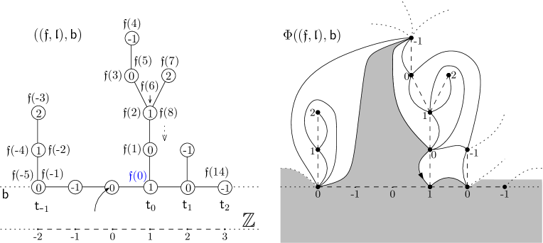
Figure 8: The Bouttier-Di Francesco-Guitter mapping applied to an element $((\textup{$\mathfrak{f}$},\textup{$\mathfrak{l}$}),\textup{{b}})\in\textup{$\mathfrak{F}$}_{\infty}\times\textup{$\mathfrak{B}$}_{\infty}$. On the right-hand side, the arcs connect the vertices $\textup{$\mathfrak{f}$}(i)$ with $\textup{$\mathfrak{f}$}(\textup{succ}_{\infty}(i))$, for $i\in\mathbb{Z}$. The other vertices and edges of the representation of $((\textup{$\mathfrak{f}$},\textup{$\mathfrak{l}$}),\textup{{b}})$ on the left-hand side do not appear in the quadrangulation. The oriented arc on the right indicated by an arrow represents the root edge of the map.

Similarly to the finite case, the vertex set of $\textup{$\mathsf{q}$}=\Phi((\textup{$\mathfrak{f}$},\textup{$\mathfrak{l}$}),\textup{{b}})$ is given by $V(\textup{$\mathfrak{f}$})$; here, we add no additional vertex. For specifying the edges, we let the successor $\textup{succ}_{\infty}(i)$ of $i\in\mathbb{Z}$ be the smallest number $k>i$ such that $\textup{$\mathfrak{L}$}_{\textup{$\mathfrak{f}$}}(k)=\textup{$\mathfrak{L}$}_{\textup{$\mathfrak{f}$}}(i)-1$. Since by assumption $\inf_{i\in\mathbb{N}}\textup{{b}}(i)=-\infty$, $\textup{succ}_{\infty}(i)$ is a finite number. We next connect the vertices $\textup{$\mathfrak{f}$}(i)$ and $\textup{$\mathfrak{f}$}(\textup{succ}_{\infty}(i))$ by an arc for any $i\in\mathbb{Z}$, such that the resulting map is planar. The arcs form the edges of the infinite rooted quadrangulation $\mathsf{q}$ we are about to construct. In order to root the map, we observe that the bi-infinite line $\mathbb{Z}$ is in correspondence with the boundary edges of $\mathsf{q}$, and we choose the edge corresponding to $\{0,1\}$ as the root edge of $\mathsf{q}$ (oriented such that the outer face lies to its right). A representation of $((\textup{$\mathfrak{f}$},\textup{$\mathfrak{l}$}),\textup{{b}})$ and of the resulting quadrangulation $\Phi((\textup{$\mathfrak{f}$},\textup{$\mathfrak{l}$}),\textup{{b}})$ is depicted in Figure 8.

4.3 Definition of the ${\textup{{UIHPQ}}}_{p}$

We are now in position to construct the $\textup{{UIHPQ}}_{p}$ by means of the above mapping $\Phi$ applied to a (random) element in $\textup{$\mathfrak{F}$}_{\infty}\times\textup{$\mathfrak{B}$}_{\infty}$, which we introduce first.

Let $\mathsf{t}$ be a finite random plane tree. Conditionally on $\mathsf{t}$, we assign to $\mathsf{t}$ a random uniform labeling $\ell$ of its vertices, so that the pair $(\mathsf{t},\ell)$ becomes a well-labeled tree. Namely, given $\mathsf{t}$, we first equip each edge of $\mathsf{t}$ with an independent random variable uniformly distributed in $\{-1,0,1\}$. Then we define the label $\ell(u)$ of a vertex $u\in V(\mathsf{t})$ to be the sum over all labels along the unique (non-backtracking) path from the tree root to $u$.

We consider Galton-Watson trees with a (sub-)critical geometric offspring law $\mu_{p}$ of parameter $1-p$ with $p\in[0,1/2]$, that is, $\mu_{p}(k)=p^{k}(1-p)$, $k\in\mathbb{N}_{0}.$ If $\mathsf{t}$ is such a tree, we call it a $p$-Galton-Watson tree. Equipped with a random uniform labeling $\ell$ as described before, we say that the pair $(\mathsf{t},(\ell(u))_{u\in V(\mathsf{t})})$ is a uniformly labeled $p$-Galton-Watson tree.

A uniformly labeled infinite $p$-forest is a random element $(\textup{$\mathfrak{f}$}_{\infty}^{(p)},\textup{$\mathfrak{l}$}_{\infty}^{(p)})$ taking values in $\textup{$\mathfrak{F}$}_{\infty}$, such that $(\mathsf{t}_{i},\textup{$\mathfrak{l}$}_{\infty}^{(p)}\restriction V(\mathsf{t}_{i}))$, $i\in\mathbb{Z}$, are independent uniformly labeled $p$-Galton-Watson trees.

A uniform infinite bridge is a random element $\textup{{b}}_{\infty}=(\textup{{b}}_{\infty}(i),i\in\mathbb{Z})$ in $\textup{$\mathfrak{B}$}_{\infty}$ such that $\textup{{b}}_{\infty}$ has the law of a two-sided simple symmetric random walk starting from $\textup{{b}}_{\infty}(0)=0$. We stress that our wording differs from [8], where a uniform infinite bridge refers to a two-sided random walk with a geometric offspring law of parameter $1/2$. See also Lemma 2 below.

Definition 5.

Fix $p\in[0,1/2]$. Let $(\textup{$\mathfrak{f}$}_{\infty}^{(p)},\textup{$\mathfrak{l}$}_{\infty}^{(p)})$ be a uniformly labeled infinite $p$-forest, and independently of $(\textup{$\mathfrak{f}$}_{\infty}^{(p)},\textup{$\mathfrak{l}$}_{\infty}^{(p)})$, let $\textup{{b}}_{\infty}$ be a uniform infinite bridge. Then the $\textup{{UIHPQ}}_{p}$ with skewness parameter $p$ is given by the (rooted) random infinite quadrangulation $Q_{\infty}^{\infty}(p)=(V(Q_{\infty}^{\infty}(p)),d_{\textup{gr}},\rho)$ with an infinite boundary, which is obtained from applying the Bouttier-Di Francesco-Guitter mapping $\Phi$ to $((\textup{$\mathfrak{f}$}_{\infty}^{(p)},\textup{$\mathfrak{l}$}_{\infty}^{(p)}),\textup{{b}}_{\infty})$. In case $p=1/2$, we simply write $Q_{\infty}^{\infty}$, which denotes then the (standard) uniform infinite half-planar quadrangulation with a general boundary.

Remark 9.

Let $\textup{$\mathfrak{f}$}_{\infty}^{(p)}$ be the encoding forest of the $\textup{{UIHPQ}}_{p}$. Instead of working with metric balls around the root vertex in the $\textup{{UIHPQ}}_{p}$, it will – due to the specific construction of the latter – often be more practical to consider metric balls around the vertex corresponding to the tree root $\textup{$\mathfrak{f}$}_{\infty}^{(p)}(0)$ in the $\textup{{UIHPQ}}_{p}$. Similarly, if $Q_{n}^{\sigma}\in\mathcal{Q}_{n}^{\sigma}$ is a uniform quadrangulation and $\textup{$\mathfrak{f}$}_{n}$ its encoding forest, it will be more natural to consider balls around $\textup{$\mathfrak{f}$}_{n}(0)$ in $Q_{n}^{\sigma}$. Since the distance between $\textup{$\mathfrak{f}$}_{\infty}^{(p)}(0)$ or $\textup{$\mathfrak{f}$}_{n}(0)$ and the root of the map is stochastically bounded (it may also be zero), this makes no difference in terms of scaling limits whatsoever; see [8, Lemma 5.6]. We shall use the notation $B^{(0)}_{r}(Q_{\infty}^{\infty}(p))$ for the metric ball of radius $r$ around $\textup{$\mathfrak{f}$}_{\infty}^{(p)}(0)$ in the $\textup{{UIHPQ}}_{p}$. Analogously, we define $B^{(0)}_{r}(Q_{n}^{\sigma})$.

5 Proofs of the limit results

5.1 The ${\textup{{UIHPQ}}}_{p}$ as a local limit of uniform quadrangulations

In this part, we prove Theorem 1 and Proposition 1. We begin with the former. The case $p=1/2$ has already been treated in [8], and the case $p=0$ will be considered afterwards, so we first fix $0<p<1/2$ and let $(\sigma_{n},n\in\mathbb{N})$ be a sequence of positive integers satisfying $\sigma_{n}=\frac{1-2p}{p}n+o(n)$. Recall that rooted pointed quadrangulations in $\mathcal{Q}_{n}^{\sigma_{n},\bullet}$ are in one-to-one correspondence with elements in $\textup{$\mathfrak{F}$}_{\sigma_{n}}^{n}\times\textup{$\mathfrak{B}$}_{\sigma_{n}}$. For proving Theorem 1, the key step is to control the law of the first $k$ trees in a forest $\textup{$\mathfrak{f}$}_{n}$ chosen uniformly at random in $\textup{$\mathfrak{F}$}_{\sigma_{n}}^{n}$, for $k$ arbitrarily large but fixed. We will see in Lemma 1 below that their law is close to the law of $k$ independent $p$-Galton-Watson trees when $n$ is sufficiently large. Together with a convergence result of bridges (Lemma 2), this allows us to couple contour and label functions of $Q_{n}^{\sigma_{n}}$ and the $\textup{{UIHPQ}}_{p}$, such that with high probability, we have equality of balls of a constant radius around the roots in $Q_{n}^{\sigma_{n}}$ and the $\textup{{UIHPQ}}_{p}$, respectively. This readily implies the theorem.

We begin with the necessary control over the trees. Since the result on the tree convergence is of some interest on its own, we formulate an optimal version, which is stronger than we what need for mere local convergence as stated in Theorem 1.

Lemma 1.

Fix $0<p<1/2$, and let $(\sigma_{n},n\in\mathbb{N})$ be a sequence of positive integers satisfying $\sigma_{n}=\frac{1-2p}{p}n+o(n)$. Let $(\mathsf{t}_{i})_{1\leq i\leq\sigma_{n}}$ be a family of $\sigma_{n}$ independent $1/2$-Galton-Watson trees, and let $(\mathsf{t}_{i}^{(p)})_{1\leq i\leq\sigma_{n}}$ be a family of $\sigma_{n}$ independent $p$-Galton-Watson trees. Then, if $(k_{n},n\in\mathbb{N})$ is a sequence of positive integers satisfying $k_{n}\leq\sigma_{n}$ and $k_{n}=o\left(n\right)$ as $n\rightarrow\infty$, we have

$$\lim_{n\rightarrow\infty}\left\|\textup{Law}\Big{(}(\mathsf{t}_{i})_{1\leq i\leq k_{n}}\,\Big{|}\,\sum_{i=1}^{\sigma_{n}}|\mathsf{t}_{i}|=n\Big{)}-\textup{Law}\left((\mathsf{t}_{i}^{(p)})_{1\leq i\leq k_{n}}\right)\right\|_{\textup{TV}}=0.$$

Remark 10.

We stress that in particular, we can choose $k_{n}$ equals an arbitrary large constant $k\in\mathbb{N}$. This suffices to show local convergence towards the $\textup{{UIHPQ}}_{p}$; see Proposition 4 below. Lemma 1 may be seen as a complement to the results on coupling of trees in [8]; it treats a regime not considered in that work.

Proof.

Let $(S^{(p)}(m),m\in\mathbb{N}_{0})$ be a random walk on the integers starting from $S^{(p)}(0)=0$ with increments distributed according to $p\delta_{1}+(1-p)\delta_{-1}$. Set, for $\ell\in\mathbb{Z}$,

$$T^{(p)}_{\ell}=\inf\left\{m\in\mathbb{N}:S^{(p)}(m)=\ell\right\}.$$

We also let $(S(m),m\in\mathbb{N}_{0})$ be a simple symmetric random walk started from $S(0)=0$ and write $T_{\ell}$ for its first hitting time of $\ell\in\mathbb{Z}$. By the encoding of a forest by its contour function described in Section 4.1.2, the claim of the lemma boils down to

$$\sup_{\ell\in\mathbb{N}}\sup_{\mathbf{x}=(x_{0},\ldots,x_{l})\in\mathbb{Z}^{\ell+1}}\Big{|} \mathbb{P}\left(T^{(p)}_{-k_{n}}=\ell,\ \left(S^{(p)}(0),\ldots,S^{(p)}(\ell)\right)=\mathbf{x}\right)$$ (3)

$$-\mathbb{P}\left(T_{-k_{n}}=\ell,\ \left(S(0),\ldots,S(\ell)\right)=\mathbf{x}\ \big{|}\ T_{-\sigma_{n}}=2n+\sigma_{n}\right)\Big{|}\longrightarrow 0$$

as $n\rightarrow\infty$. First, observe that $S(1)$ can be obtained as the Cramér transform of $S^{(p)}(1)$, meaning that

$$\mathbb{P}(S(1)=k)=\frac{\lambda_{p}^{k}}{G(p)}\mathbb{P}\left(S^{(p)}(1)=k\right),\quad k\in\{-1,1\},$$

where $\lambda_{p}=\sqrt{\tfrac{1-p}{p}}$ and $G(p)=p\lambda_{p}+(1-p)/\lambda_{p}$. Let us fix $\ell\in\mathbb{N}$ and $\mathbf{x}\in\mathbb{Z}^{\ell+1}$. We have

$$\mathbb{P}\left(T_{-k_{n}}=\ell,\ \left(S(0),\ldots,S(\ell)\right)=\mathbf{x},\ T_{-\sigma_{n}}=2n+\sigma_{n}\right)$$

$$\qquad=\sum_{\gamma}\prod_{j=1}^{2n+\sigma_{n}}{\mathbb{P}\left(S(j)-S(j-1)=\gamma_{j}-\gamma_{j-1}\right)}$$

$$\qquad=\frac{\lambda_{p}^{-\sigma_{n}}}{(G(p))^{2n+\sigma_{n}}}\sum_{\gamma}\prod_{j=1}^{2n+\sigma_{n}}{\mathbb{P}\left(S^{(p)}(j)-S^{(p)}(j-1)=\gamma_{j}-\gamma_{j-1}\right)}$$

$$\qquad=\frac{\lambda_{p}^{-\sigma_{n}}}{(G(p))^{2n+\sigma_{n}}}\mathbb{P}\left(T^{(p)}_{-k_{n}}=\ell,\ \left(S^{(p)}(0),\ldots,S^{(p)}(\ell)\right)=\mathbf{x},\ T^{(p)}_{-\sigma_{n}}=2n+\sigma_{n}\right),$$

where the sums are over all paths $\gamma:\{0,\ldots,2n+\sigma_{n}\}\rightarrow\mathbb{Z}$ for which the probabilities on the right-hand side are non-zero. By the same argument, we obtain

$$\mathbb{P}\left(T_{-\sigma_{n}}=2n+\sigma_{n}\right)=\frac{\lambda_{p}^{-\sigma_{n}}}{(G(p))^{2n+\sigma_{n}}}\mathbb{P}\left(T^{(p)}_{-\sigma_{n}}=2n+\sigma_{n}\right),$$

so that finally

$$\mathbb{P}\left(T_{-k_{n}}=\ell,\ \left(S(0),\ldots,S(\ell)\right)=\mathbf{x}\ \big{|}\ T_{-\sigma_{n}}=2n+\sigma_{n}\right)$$

$$\qquad=\mathbb{P}\left(T^{(p)}_{-k_{n}}=\ell,\ \left(S^{(p)}(0),\ldots,S^{(p)}(\ell)\right)=\mathbf{x}\ \big{|}\ T^{(p)}_{-\sigma_{n}}=2n+\sigma_{n}\right).$$

By applying the Markov property at time $T^{(p)}_{-k_{n}}$, we have

$$\mathbb{P}\left(T^{(p)}_{-k_{n}}=\ell,\ \left(S^{(p)}(0),\ldots,S^{(p)}(\ell)\right)=\mathbf{x}\ \big{|}\ T^{(p)}_{-\sigma_{n}}=2n+\sigma_{n}\right)$$

$$\qquad=\frac{1}{\mathbb{P}\left(\ T^{(p)}_{-\sigma_{n}}=2n+\sigma_{n}\right)}\mathbb{E}\left(\mathbf{1}_{\left\{T^{(p)}_{-k_{n}}=\ell,\ \left(S^{(p)}(0),\ldots,S^{(p)}(\ell)\right)=\mathbf{x}\right\}}\mathbb{P}\left(T^{(p)}_{-\sigma_{n}}=2n+\sigma_{n}\ \big{|}\ T^{(p)}_{-k_{n}}=\ell\right)\right)$$

$$\qquad=\mathbb{P}\left(T^{(p)}_{-k_{n}}=\ell,\ \left(S^{(p)}(0),\ldots,S^{(p)}(\ell)\right)=\mathbf{x}\right)\frac{\mathbb{P}\left(T^{(p)}_{-\sigma_{n}+k_{n}}=2n+\sigma_{n}-\ell\right)}{\mathbb{P}\left(\ T^{(p)}_{-\sigma_{n}}=2n+\sigma_{n}\right)}\,.$$

Note that we can assume, without loss of generality, that $k_{n}\rightarrow\infty$ as $n\rightarrow\infty$. Now, by the law of large numbers, since $(S^{(p)}(m),m\in\mathbb{N}_{0})$ has negative drift we have that

$$\mathbb{P}\left(T^{(p)}_{-k_{n}}>Mk_{n}\right)\leq\mathbb{P}\left(S^{(p)}_{Mk_{n}}>-k_{n}\right)=\mathbb{P}\left(\frac{S^{(p)}_{Mk_{n}}}{Mk_{n}}>-\frac{1}{M}\right)\longrightarrow 0$$

as $n\rightarrow\infty$, provided that $M$ is large enough. As a consequence, we may restrict ourselves to the values $\ell\in\{1,\ldots,Mk_{n}\}$. By Kemperman’s formula [37, Section 6.1], we get

$$\frac{\mathbb{P}\left(T^{(p)}_{-\sigma_{n}+k_{n}}=2n+\sigma_{n}-\ell\right)}{\mathbb{P}\left(\ T^{(p)}_{-\sigma_{n}}=2n+\sigma_{n}\right)}=\frac{\sigma_{n}-k_{n}}{2n+\sigma_{n}-\ell}\cdot\frac{2n+\sigma_{n}}{\sigma_{n}}\cdot\frac{\mathbb{P}\left(S^{(p)}_{2n+\sigma_{n}-\ell}=-\sigma_{n}+k_{n}\right)}{\mathbb{P}\left(S^{(p)}_{2n+\sigma_{n}}=-\sigma_{n}\right)}.$$

Since we assumed that $\ell\leq Mk_{n}$ and $k_{n}=o(\sigma_{n})$ we have

$$\lim_{n\rightarrow\infty}{\frac{\sigma_{n}-k_{n}}{2n+\sigma_{n}-\ell}}=\lim_{n\rightarrow\infty}{\frac{\sigma_{n}}{2n+\sigma_{n}}}=1-2p,$$

so that by the local limit theorem (see [28] for instance),

$$\sup_{1\leq\ell\leq Mk_{n}}\frac{\mathbb{P}\left(S^{(p)}_{2n+\sigma_{n}-\ell}=-\sigma_{n}+k_{n}\right)}{\mathbb{P}\left(S^{(p)}_{2n+\sigma_{n}}=-\sigma_{n}\right)}\longrightarrow 1$$

as $n\rightarrow\infty$, which yields (3) and completes the proof. ∎

We continue with a convergence result for uniform bridges $\textup{{b}}_{n}\in\textup{$\mathfrak{B}$}_{\sigma_{n}}$ towards $\textup{{b}}_{\infty}$.

Lemma 2.

Let $(\sigma_{n},n\in\mathbb{N})$ be a sequence of positive integers satisfying $\sigma_{n}\rightarrow\infty$ as $n\rightarrow\infty$. Let $\textup{{b}}_{n}$ be uniformly distributed in $\textup{$\mathfrak{B}$}_{\sigma_{n}}$, and let $\textup{{b}}_{\infty}$ be a uniform infinite bridge as specified in Section 4. Then, if $k_{n}$ is a sequence of positive integers with $k_{n}\leq\sigma_{n}$ and $k_{n}=o(\sigma_{n})$ as $n\rightarrow\infty$,

$$\begin{split}\lim_{n\rightarrow\infty}&\left\|\textup{Law}((\textup{{b}}_{n}(2\sigma_{n}-k_{n}),\ldots,\textup{{b}}_{n}(2\sigma_{n}-1),\textup{{b}}_{n}(0),\textup{{b}}_{n}(1),\ldots,\textup{{b}}_{n}(k_{n})))\right.\\ &\left.-\,\textup{Law}((\textup{{b}}_{\infty}(-k_{n}),\ldots,\textup{{b}}_{\infty}(-1),\textup{{b}}_{\infty}(0),\textup{{b}}_{\infty}(1),\ldots,\textup{{b}}_{\infty}(k_{n})))\right\|_{\textup{TV}}=0.\end{split}$$

The proof follows from a small adaption of [8, Proof of Lemma 5.5] and is left to the reader. Roughly speaking, it relies on the exact computation of the probability that $(\textup{{b}}_{n}(2\sigma_{n}-k_{n}),\ldots,\textup{{b}}_{n}(2\sigma_{n}-1),\textup{{b}}_{n}(0),\ldots,\textup{{b}}_{n}(k_{n}))$ and $(\textup{{b}}_{\infty}(-k_{n}),\ldots,\textup{{b}}_{\infty}(-1),\textup{{b}}_{\infty}(0),\ldots,\textup{{b}}_{\infty}(k_{n}))$ equal a fixed sequence $(x_{0},\ldots,x_{2k_{n}-1})\in\mathbb{Z}^{2k_{n}}$, which involves binomial coefficients by definition of bridges. We stress, however, that in [8], $\textup{{b}}_{n}$ and $\textup{{b}}_{\infty}$ were defined in a slightly different manner, by grouping the $+1$-steps between two subsequent down-steps together to one “big” jump. Clearly, this does change the argument only in a minor way.

We are now in position to formulate an appropriate coupling of balls.

Proposition 4.

Fix $0<p<1/2$, and let $(\sigma_{n},n\in\mathbb{N})$ be a sequence of positive integers satisfying $\sigma_{n}=\frac{1-2p}{p}n+o(n)$. Let also $(\xi_{n},n\in\mathbb{N})$ be a sequence of positive integers satisfying $\xi_{n}=o(\sqrt{n})$. Then, given any $\varepsilon>0$, there exist $\delta>0$ and $n_{0}\in\mathbb{N}$ such that for every $n\geq n_{0}$, we can construct on the same probability space copies of $Q_{n}^{\sigma_{n}}$ and the $\textup{{UIHPQ}}_{p}$ such that with probability at least $1-\varepsilon$, the metric balls $B_{\delta\xi_{n}}(Q_{n}^{\sigma_{n}})$ and $B_{\delta\xi_{n}}(\textup{{UIHPQ}}_{p})$ of radius $\delta\xi_{n}$ around the roots in the corresponding spaces are isometric.

The local convergence of $Q_{n}^{\sigma_{n}}$ towards $\textup{{UIHPQ}}^{(p)}$ is a weaker statement, hence Theorem 1 in the case $0<p<1/2$ will follow from the proposition.

Proof.

The proof is in spirit of [8, Proof of Proposition 3.11], requires, however, some modifications. We will indicate at which place we may simply adapt the reasoning. We consider a random uniform element $((\textup{$\mathfrak{f}$}_{n},\textup{$\mathfrak{l}$}_{n}),\textup{{b}}_{n})\in\textup{$\mathfrak{F}$}_{\sigma_{n}}^{n}$, and a triplet $((\textup{$\mathfrak{f}$}_{\infty}^{(p)},\textup{$\mathfrak{l}$}_{\infty}^{(p)}),\textup{{b}}_{\infty})$ consisting of a uniformly labeled infinite $p$-forest together with an (independent) uniform infinite bridge $\textup{{b}}_{\infty}$. We let $(Q_{n}^{\sigma_{n}},v^{\bullet})=\Phi_{n}((\textup{$\mathfrak{f}$}_{n},\textup{$\mathfrak{l}$}_{n}),\textup{{b}}_{n})$ and $Q_{\infty}^{\infty}(p)=\Phi((\textup{$\mathfrak{f}$}_{\infty}^{(p)},\textup{$\mathfrak{l}$}_{\infty}^{(p)}),\textup{{b}}_{\infty})$ be the quadrangulations obtained from applying the Bouttier-Di Francesco-Guitter mapping to $((\textup{$\mathfrak{f}$}_{n},\textup{$\mathfrak{l}$}_{n}),\textup{{b}}_{n})$ and $((\textup{$\mathfrak{f}$}_{\infty}^{(p)},\textup{$\mathfrak{l}$}_{\infty}^{(p)}),\textup{{b}}_{\infty})$, respectively. Recall that $\textup{$\mathfrak{f}$}_{n}=(\mathsf{t}_{0},\ldots,\mathsf{t}_{\sigma_{n}-1})$ consists of $\sigma_{n}$ trees. For $0\leq k\leq\sigma_{n}-1$, we let $\mathsf{t}(\textup{$\mathfrak{f}$}_{n},k)=\mathsf{t}_{k}$, i.e., $\mathsf{t}(\textup{$\mathfrak{f}$}_{n},k)$ is the tree of $\textup{$\mathfrak{f}$}_{n}$ with index $k$, and we put $\mathsf{t}(\textup{$\mathfrak{f}$}_{n},\sigma_{n})=\mathsf{t}(\textup{$\mathfrak{f}$}_{n},0)$. In a similar manner, $\mathsf{t}(\textup{$\mathfrak{f}$}_{\infty}^{(p)},k)$ denotes the tree of $\textup{$\mathfrak{f}$}_{\infty}^{(p)}$ indexed by $k\in\mathbb{Z}$.

By Lemma 1, we find $\delta^{\prime}>0$ and $n^{\prime}_{0}\in\mathbb{N}$ such that for $n\geq n^{\prime}_{0}$, we can construct $((\textup{$\mathfrak{f}$}_{n},\textup{$\mathfrak{l}$}_{n}),\textup{{b}}_{n})$ and $((\textup{$\mathfrak{f}$}_{\infty}^{(p)},\textup{$\mathfrak{l}$}_{\infty}^{(p)}),\textup{{b}}_{\infty})$ on the same probability space such that with $A_{n}=\lfloor\delta^{\prime}\xi_{n}^{2}\rfloor$, the event

$$\mathcal{E}^{1}(n,\delta^{\prime}) =\quad\left\{\mathsf{t}(\textup{$\mathfrak{f}$}_{n},i)=\mathsf{t}(\textup{$\mathfrak{f}$}_{\infty}^{(p)},i),\,\mathsf{t}(\textup{$\mathfrak{f}$}_{n},\sigma_{n}-i)=\mathsf{t}(\textup{$\mathfrak{f}$}_{\infty}^{(p)},-i)\textup{ for all }0\leq i\leq A_{n}\right\}$$

$$\,\quad\cap\left\{\textup{$\mathfrak{l}$}_{n}|_{\mathsf{t}(\textup{$\mathfrak{f}$}_{n},i)}=\textup{$\mathfrak{l}$}_{\infty}^{(p)}|_{\mathsf{t}(\textup{$\mathfrak{f}$}_{\infty}^{(p)},i)},\,\textup{$\mathfrak{l}$}_{n}|_{\mathsf{t}(\textup{$\mathfrak{f}$}_{n},\sigma_{n}-i)}=\textup{$\mathfrak{l}$}_{\infty}^{(p)}|_{\mathsf{t}(\textup{$\mathfrak{f}$}_{\infty}^{(p)},-i)}\textup{ for all }0\leq i\leq A_{n}\right\}$$

has probability at least $1-\varepsilon/8$. We now fix such a $\delta^{\prime}$ for the rest of the proof. Recall that by our construction of the Bouttier-Di Francesco-Guitter bijection, the trees of $\textup{$\mathfrak{f}$}_{n}$ are attached to the down-steps $\textup{d}^{\downarrow}_{n}(i)=\textup{d}^{\downarrow}_{\textup{{b}}_{n}}(i)$ of $\textup{{b}}_{n}$, $1\leq i\leq\sigma_{n}$, and similarly, the trees of $\textup{$\mathfrak{f}$}_{\infty}^{(p)}$ are attached to the down-steps $\textup{d}^{\downarrow}_{\infty}(i)=\textup{d}^{\downarrow}_{\textup{{b}}_{\infty}}(i)$ of $\textup{{b}}_{\infty}$, where now $i\in\mathbb{Z}$. In view of the above event, this incites us to consider additionally the event

$$\mathcal{E}^{2}(n,\delta^{\prime}) =\quad\left\{\textup{{b}}_{n}(i)=\textup{{b}}_{\infty}(i)\textup{ for all }1\leq i\leq\textup{d}^{\downarrow}_{\infty}(A_{n}+1)\right\}$$

$$\,\quad\cap\left\{\textup{{b}}_{n}(2\sigma_{n}+i)=\textup{{b}}_{\infty}(i)\textup{ for all }\textup{d}^{\downarrow}_{\infty}(-A_{n})\leq i\leq-1\right\}.$$

Note that on $\mathcal{E}^{2}(n,\delta^{\prime})$, we automatically have $\textup{d}^{\downarrow}_{n}(i)=\textup{d}^{\downarrow}_{\infty}(i)$ for $1\leq i\leq A_{n}+1$, and $\textup{d}^{\downarrow}_{n}(\sigma_{n}-i+1)=\textup{d}^{\downarrow}_{\infty}(-i)$ for $1\leq i\leq A_{n}$. Trivially, we have that $\textup{d}^{\downarrow}_{\infty}(A_{n}+1)\geq A_{n}+1$ and $\textup{d}^{\downarrow}_{\infty}(-A_{n})\leq-A_{n}$, but also, with probability tending to $1$, $\textup{d}^{\downarrow}_{\infty}(A_{n}+1)\leq 3A_{n}$ and $\textup{d}^{\downarrow}_{\infty}(-A_{n})\geq-3A_{n}$. Since, in any case, $A_{n}=o(\sigma_{n})$, we can ensure by Lemma 2 that the event $\mathcal{E}^{2}(n,\delta^{\prime})$ has probability at least $1-\varepsilon/8$ for large $n$.

Now for $\delta>0$, $n\in\mathbb{N}$, define the events

$$\mathcal{E}^{3}(n,\delta)=\left\{\min_{[0,\,\textup{d}^{\downarrow}_{\infty}(A_{n}+1)]}\textup{{b}}_{\infty}<-5\delta\xi_{n},\,\min_{[\textup{d}^{\downarrow}_{\infty}(-A_{n}),-1]}\textup{{b}}_{\infty}<-5\delta\xi_{n}\right\},$$

$$\mathcal{E}^{4}(n,\delta)=\left\{\min_{[\textup{d}^{\downarrow}_{\infty}(A_{n}+1)+1,\,\textup{d}^{\downarrow}_{\infty}(-A_{n})-1]}\textup{{b}}_{n}<-5\delta\xi_{n}\right\}.$$

By invoking Donsker’s invariance principle together with Lemma 2 for the event $\mathcal{E}^{3}$ (and again the fact that $A_{n}+1\leq\textup{d}^{\downarrow}_{\infty}(A_{n}+1)\leq 3A_{n}$ and $-3A_{n}\leq\textup{d}^{\downarrow}_{\infty}(-A_{n})\leq-A_{n}$ with high probability), we deduce that for small $\delta>0$, provided $n$ is large enough,

$$\mathbb{P}\left(\mathcal{E}^{3}(n,\delta)\right)\geq 1-\varepsilon/8,\quad\textup{and}\quad\mathbb{P}\left(\mathcal{E}^{4}(n,\delta)\right)\geq 1-\varepsilon/8.$$

We will now assume that $n_{0}\geq n^{\prime}_{0}$ and $\delta>0$ are such that for all $n\geq n_{0}$, the above bounds hold true, and work on the event $\mathcal{E}^{1}(n,\delta^{\prime})\cap\mathcal{E}^{2}(n,\delta^{\prime})\cap\mathcal{E}^{3}(n,\delta)\cap\mathcal{E}^{4}(n,\delta)$ of probability at least $1-\varepsilon/2$. We consider the forest obtained from restricting $\textup{$\mathfrak{f}$}_{n}$ to the first $A_{n}+1$ and the last $A_{n}$ trees,

$$\textup{$\mathfrak{f}$}^{\prime}_{n}=\left(\mathsf{t}(\textup{$\mathfrak{f}$}_{n},0),\ldots,\mathsf{t}(\textup{$\mathfrak{f}$}_{n},A_{n}),\mathsf{t}(\textup{$\mathfrak{f}$}_{n},\sigma_{n}-A_{n}),\ldots,\mathsf{t}(\textup{$\mathfrak{f}$}_{n},\sigma_{n}-1)\right).$$

Similarly, we define ${\textup{$\mathfrak{f}$}_{\infty}^{{}^{\prime}(p)}}$. We recall the cactus bounds in the version stated in [8, (4.4) of Section 4.5]. Applied to $Q_{n}^{\sigma_{n}}$, it shows that for vertices $v\in V(\textup{$\mathfrak{f}$}_{n})\setminus V(\textup{$\mathfrak{f}$}^{\prime}_{n})$, with $d_{n}$ denoting the graph distance,

$$d_{n}(\textup{$\mathfrak{f}$}_{n}(0),v)\geq-\max\left\{\min_{[0,\,\textup{d}^{\downarrow}_{\infty}(A_{n}+1)]}\textup{{b}}_{n},\min_{[\textup{d}^{\downarrow}_{\infty}(-A_{n})\,,2\sigma_{n}]}\textup{{b}}_{n}\right\}\geq 5\delta\xi_{n}.$$

Applying now the analogous cactus bound [8, (4.6) of Section 4.5] to the infinite quadrangulation $Q_{\infty}^{\infty}(p)$, we obtain the same lower bound for vertices $v\in V(\textup{$\mathfrak{f}$}_{\infty}^{(p)})\setminus V(\textup{$\mathfrak{f}$}^{{}^{\prime}(p)}_{\infty})$, with $d_{n}$ replaced by the graph distance $d_{\infty}^{(p)}$ in $Q_{\infty}^{\infty}(p)$, and $\textup{$\mathfrak{f}$}_{n}(0)$ replaced by the vertex $\textup{$\mathfrak{f}$}_{\infty}^{(p)}(0)$ of $Q_{\infty}^{\infty}(p)$. We recall the definition of the metric balls $B_{r}^{(0)}(Q_{n}^{\sigma_{n}})$ and $B_{r}^{(0)}(Q_{\infty}^{\infty}(p))$; see Remark 9. With the same arguments as in [8, Proof of Proposition 3.11], we then deduce that vertices at a distance at most $5\delta\xi_{n}-1$ from $\textup{$\mathfrak{f}$}_{n}(0)$ in $Q_{n}^{\sigma_{n}}$ agree with those at a distance at most $5\delta\xi_{n}-1$ from $\textup{$\mathfrak{f}$}_{\infty}^{(p)}(0)$ in $Q_{\infty}^{\infty}(p)$. Moreover,

$$d_{n}(u,v)=d_{\infty}^{(p)}(u,v)\quad\hbox{whenever }u,v\in B^{(0)}_{2\delta\xi_{n}}(Q_{n}^{\sigma_{n}}).$$

This proves that the balls $B^{(0)}_{2\delta\xi_{n}}(Q_{n}^{\sigma_{n}})$ and $B^{(0)}_{2\delta\xi_{n}}(Q_{\infty}^{\infty}(p))$ are isometric on an event of probability at least $1-\varepsilon/2$. In order to conclude, it suffices to observe that the distances from $\textup{$\mathfrak{f}$}_{n}(0)$ resp. $\textup{$\mathfrak{f}$}_{\infty}^{(p)}(0)$ to the root vertex in $Q_{n}^{\sigma_{n}}$ resp. $Q_{\infty}^{\infty}(p)$ are stochastically bounded; see again Remark 9. Clearly, this implies that with probability tending to $1$ as $n$ increases, we have the inclusions $B_{\delta\xi_{n}}(Q_{n}^{\sigma_{n}})\subset B^{(0)}_{2\delta\xi_{n}}(Q_{n}^{\sigma_{n}})$ and $B_{\delta\xi_{n}}(Q_{\infty}^{\infty}(p))\subset B_{2\delta\xi_{n}}^{(0)}(Q_{\infty}^{\infty}(p))$. ∎

As mentioned at the beginning, the case $p=1/2$ has already been treated in [8, Proof of Proposition 3.11]: It is proved there that for $\delta$ small, balls of radius $\delta\min\{\sqrt{\sigma_{n}},\sqrt{n/\sigma_{n}}\}$ in $Q_{n}^{\sigma_{n}}$ and in the standard $\textup{{UIHPQ}}=\textup{{UIHPQ}}_{1/2}$ can be coupled with high probability, implying of course again local convergence of $Q_{n}^{\sigma_{n}}$ towards the UIHPQ.

Finally, it remains to consider the case $p=0$ corresponding to $\sigma_{n}\gg n$. This case is easy. We have the following coupling lemma.

Lemma 3.

Let $(\sigma_{n},n\in\mathbb{N})$ be a sequence of positive integers satisfying $\sigma_{n}\gg n$. Put $\xi_{n}=\sigma_{n}/n$. Then, given any $\varepsilon>0$, there exist $\delta>0$ and $n_{0}\in\mathbb{N}$ such that for every $n\geq n_{0}$, we can construct on the same probability space copies of $Q_{n}^{\sigma_{n}}$ and the $\textup{{UIHPQ}}_{0}$ such that with probability at least $1-\varepsilon$, the metric balls $B_{\delta\xi_{n}}(Q_{n}^{\sigma_{n}})$ and $B_{\delta\xi_{n}}(\textup{{UIHPQ}}_{0})$ of radius $\delta\xi_{n}$ around the roots in the corresponding spaces are isometric.

Proof.

Let $((\textup{$\mathfrak{f}$}_{n},\textup{$\mathfrak{l}$}_{n}),\textup{{b}}_{n})\in\textup{$\mathfrak{F}$}_{\sigma_{n}}^{n}\times\textup{$\mathfrak{B}$}_{\sigma_{n}}$ be uniformly distributed. By exchangeability of the trees, it follows that if $k_{n}=o(\sigma_{n}/n)$, then the first and last $k_{n}$ trees of $\textup{$\mathfrak{f}$}_{n}$ are all singletons with a probability tending to one. Applying Lemma 2, we can ensure that the event

$$\left\{\textup{{b}}_{n}(i)=\textup{{b}}_{\infty}(i),\,\textup{{b}}_{n}(2\sigma_{n}-i)=\textup{{b}}_{\infty}(-i),\,1\leq i\leq k_{n}\right\}$$

has a probability as large as we wish, provided $n$ is large enough. Given $\varepsilon>0$, the same arguments as in the proof of Proposition 4 yield an equality of balls $B_{\delta\xi_{n}}(Q_{n}^{\sigma_{n}})$ and $B_{\delta\xi_{n}}(\textup{{UIHPQ}}_{0})$ for $\delta$ small and $n$ large enough, on an event of probability at least $1-\varepsilon$. ∎

Let us now show that the space $\textup{{UIHPQ}}_{0}$ defined in terms of the Bouttier-Di Francesco-Guitter mapping in Section 4.3 is nothing else than Kesten’s tree associated to the critical geometric offspring law $\mu_{1/2}$.

Proof of Proposition 1.

Let $\textup{{b}}_{\infty}=(\textup{{b}}_{\infty}(i),i\in\mathbb{Z})$ be a uniform infinite bridge, and let $(\textup{$\mathfrak{f}$}_{\infty}^{(0)},\textup{$\mathfrak{l}$}_{\infty}^{(0)})$ be the infinite forest where all trees are just singletons (with label $0$); see Section 4.3. The $\textup{{UIHPQ}}_{0}$ is distributed as the infinite map $Q_{\infty}^{\infty}(0)=\Phi((\textup{$\mathfrak{f}$}_{\infty}^{(0)},\textup{$\mathfrak{l}$}_{\infty}^{(0)}),\textup{{b}}_{\infty})$. Since every vertex in $\textup{$\mathfrak{f}$}_{\infty}^{(0)}$ defines a single corner, properties of the Bouttier-Di Francesco-Guitter mapping (Section 4.2) imply that $Q_{\infty}^{\infty}(0)$ is a tree almost surely. Moreover, the set of vertices of $Q_{\infty}^{\infty}(0)$ is identified with the set of down-steps $\textup{{DS}}(\textup{{b}}_{\infty})$ of the bridge. Following [9, Section 2.2.3], conditionally on $\textup{{b}}_{\infty}$, we introduce a function $\varphi:\mathbb{Z}\rightarrow\textup{{DS}}(\textup{{b}}_{\infty})$ that associates to $i\in\mathbb{Z}$ the next down-step larger than $i$ with label $\textup{{b}}_{\infty}(i)$ (and $i$ is mapped to itself if $i\in\textup{{DS}}(\textup{{b}}_{\infty})$). According to our rooting convention, the root edge of $Q_{\infty}^{\infty}(0)$ connects $\varphi(0)$ to $\varphi(1)$. Note that $\varphi$ is not injective almost surely.

We recall that Kesten’s tree can be represented by a half-line of vertices $s_{0},s_{1},\ldots,$ together with a collection of independent Galton-Watson trees with offspring law $\mu_{1/2}$ grafted to the left and right side of each vertex $s_{i}$, $i\in\mathbb{N}_{0}$. We will now argue that the $\textup{{UIHPQ}}_{0}$ $Q_{\infty}^{\infty}(0)$ has the same structure. In this regard, let us introduce the stopping times

$$S_{i}=\inf\{k\in\mathbb{N}_{0}:\textup{{b}}_{\infty}(k)=-i\},\quad i\in\mathbb{N}_{0},$$

and denote by $s_{i}$ the vertex of $Q_{\infty}^{\infty}(0)$ given by $\varphi(S_{i})$. Together with their connecting edges, the collection $(s_{i},i\in\mathbb{N}_{0})$ forms a spine (i.e., an infinite self-avoiding path) in $Q_{\infty}^{\infty}(0)$.

The subtree rooted at $s_{i}$ on the left side of the spine is encoded by the excursion $\{\textup{{b}}_{\infty}(k):S_{i}\leq k\leq S_{i+1}\}$, in a way we describe next; see Figure 9 for an illustration. First note that by the Markov property, these subtrees for $i\in\mathbb{Z}$ are i.i.d.. In order to determine their law, let us consider the subtree encoded by the excursion $\{\textup{{b}}_{\infty}(k):0\leq k\leq S_{1}\}$ of $\textup{{b}}_{\infty}$. This subtree is rooted at $s_{0}=\emptyset$, and the number of offspring of $s_{0}$ is the number of down-steps with label $1$ between $0$ and $S_{1}$. Otherwise said, this is the number $\#\{0<k<S_{1}:\textup{{b}}_{\infty}(k)=0\}$ of excursions of $\textup{{b}}_{\infty}$ above $0$ between $0$ and $S_{1}$. By the Markov property, this quantity follows the geometric distribution $\mu_{1/2}$ of parameter $1/2$. One can now repeat the argument for each child of $s_{0}$, by considering the corresponding excursion above $0$ encoding its progeny tree, inside the mother excursion. We obtain that the subtree stemming from $s_{0}$ on the left of the spine has indeed the law of a Galton-Watson tree with offspring distribution $\mu_{1/2}$.

The subtrees attached to the vertices $s_{i}$, $i\in\mathbb{N}_{0}$, on the right of the spine can be treated by a symmetry argument. Namely, letting

$$S^{\prime}_{i}=\inf\{k\in\mathbb{N}_{0}:\textup{{b}}_{\infty}(-k)=-i\},\quad i\in\mathbb{N}_{0},$$

we observe that the subtree rooted at $s_{i}$ to the right of the spine is coded by the (reversed) excursion $\{\textup{{b}}_{\infty}(k):-S^{\prime}_{i+1}\leq k\leq-S^{\prime}_{i}\}$. With the same argument as above, we see that it has the law of an (independent) $\mu_{1/2}$-Galton Watson tree. This concludes the proof. ∎

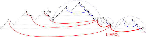
Figure 9: The construction of the $\textup{{UIHPQ}}_{0}$ from a uniform infinite bridge $\textup{{b}}_{\infty}$. The spine is shown in bold red arcs. The trees on the left of the spine are drawn in blue and enclosed by dotted blue half-circles, which indicate the corresponding excursions of $\textup{{b}}_{\infty}$ encoding these trees. The trees on the right of the spine are drawn in red, as the spine itself.

5.2 The ${\textup{{UIHPQ}}_{p}}$ as a local limit of Boltzmann quadrangulations

This section is devoted to the proof of Proposition 2. It is convenient to first prove the analogous result for pointed maps. For that purpose, we first extend the definitions of Boltzmann measures from Section 1.2.5 to pointed maps and then use a “de-pointing” argument. We use the notation $\mathcal{Q}_{f}^{\bullet}$ for the set of finite rooted pointed quadrangulations, and we write $\mathcal{Q}^{\bullet,\sigma}_{f}$ for the set of finite pointed rooted quadrangulations with $2\sigma$ boundary edges. The corresponding partition functions read

$$F^{\bullet}(g,z)=\sum_{\textup{$\mathsf{q}$}\in\mathcal{Q}_{f}^{\bullet}}g^{\#\textup{F}(\textup{$\mathsf{q}$})}z^{\#\partial\textup{$\mathsf{q}$}/2},\quad F^{\bullet}_{\sigma}(g)=\sum_{\textup{$\mathsf{q}$}\in\mathcal{Q}^{\bullet,\sigma}_{f}}g^{\#\textup{F}(\textup{$\mathsf{q}$})},$$

and the associated pointed Boltzmann distributions are defined by

$$\mathbb{P}_{g,z}^{\bullet}(\textup{$\mathsf{q}$})=\frac{g^{\#\textup{F}(\textup{$\mathsf{q}$})}z^{\#\partial\textup{$\mathsf{q}$}/2}}{F^{\bullet}(g,z)},\quad\textup{$\mathsf{q}$}\in\mathcal{Q}_{f}^{\bullet},\quad\mathbb{P}_{g}^{\bullet,\sigma}(\textup{$\mathsf{q}$})=\frac{g^{\#\textup{F}(\textup{$\mathsf{q}$})}}{F^{\bullet}_{\sigma}(g)},\quad\textup{$\mathsf{q}$}\in\mathcal{Q}^{\bullet,\sigma}_{f}.$$

We will need the following enumeration result for pointed rooted maps. From [16, (23)] and [15, Section 3.3], we have for every $0\leq p\leq 1/2$

$$F_{\sigma}^{\bullet}(g_{p})=\binom{2\sigma}{\sigma}\left(\frac{1}{1-p}\right)^{\sigma},\quad\sigma\in\mathbb{N}_{0}.$$ (4)

Note that the result (3.29) in [15] cannot be used directly, due to a difference in the rooting convention (there, the root vertex has to be chosen among the vertices of the boundary that are closest to the marked point).

Recall that $g_{p}=p(1-p)/3$ for $0\leq p\leq 1/2$. The first step towards the proof of Proposition 2 is the following convergence result for pointed Boltzmann quadrangulations.

Proposition 5.

Let $0\leq p\leq 1/2$. For every $\sigma\in\mathbb{N}_{0}$, let $Q^{\bullet}_{\sigma}(p)$ be a random rooted pointed quadrangulation distributed according to $\mathbb{P}^{\bullet,\sigma}_{g_{p}}$. Then, we have the local convergence for the metric $d_{\textup{map}}$ as $\sigma\to\infty$

$$Q_{\sigma}^{\bullet}(p)\overset{(d)}{\longrightarrow}\textup{{UIHPQ}}_{p},$$

Proof.

Let $\textup{$\mathsf{q}$}\in\mathcal{Q}^{\sigma}_{f}$, and $((\textup{$\mathfrak{f}$},\textup{$\mathfrak{l}$}),\textup{{b}})\in\cup_{n\geq 0}{\textup{$\mathfrak{F}$}_{\sigma}^{n}}\times\textup{$\mathfrak{B}$}_{\sigma}$ such that $\textup{$\mathsf{q}$}=\Phi((\textup{$\mathfrak{f}$},\textup{$\mathfrak{l}$}),\textup{{b}})$. Moreover, let $(\textup{$\mathfrak{f}$}_{\sigma}^{(p)},\textup{$\mathfrak{l}$}_{\sigma}^{(p)})$ be a uniformly labeled $p$-forest with $\sigma$ trees, i.e., a collection of $\sigma$ independent uniformly labeled $p$-Galton-Watson trees, and let $\textup{{b}}_{\sigma}$ be uniformly distributed in $\textup{$\mathfrak{B}$}_{\sigma}$ and independent of $(\textup{$\mathfrak{f}$}_{\sigma}^{(p)},\textup{$\mathfrak{l}$}_{\sigma}^{(p)})$. We have

$$\mathbb{P}\left(\Phi\big{(}(\textup{$\mathfrak{f}$}_{\sigma}^{(p)},\textup{$\mathfrak{l}$}_{\sigma}^{(p)}),\textup{{b}}_{\sigma}\big{)}=\textup{$\mathsf{q}$}\right) =\mathbb{P}\left(\big{(}(\textup{$\mathfrak{f}$}_{\sigma}^{(p)},\textup{$\mathfrak{l}$}_{\sigma}^{(p)}),\textup{{b}}_{\sigma}\big{)}=\left(\left(\textup{$\mathfrak{f}$},\textup{$\mathfrak{l}$}\right),\textup{{b}}\right)\right)$$

$$=\left(\frac{p(1-p)}{3}\right)^{|\textup{$\mathfrak{f}$}|}\frac{(1-p)^{\sigma}}{\binom{2\sigma}{\sigma}}=\frac{g_{p}^{\#\textup{F}(\textup{$\mathsf{q}$})}}{F_{\sigma}^{\bullet}(g_{p})},$$

Here, for the first equality in the second line, we have used (2), the fact that the label differences are i.i.d. uniform in $\{-1,0,1\}$, and $|\textup{$\mathfrak{B}$}_{\sigma}|=\binom{2\sigma}{\sigma}$. The last equality follows from the enumeration result (4) and the fact that the number of edges of $\mathfrak{f}$ equals the number of faces of $\mathsf{q}$. Thus, $Q^{\bullet}_{\sigma}(p)$ is distributed as $\Phi((\textup{$\mathfrak{f}$}_{\sigma}^{(p)},\textup{$\mathfrak{l}$}_{\sigma}^{(p)}),\textup{{b}}_{\sigma})$.

Now observe that $\textup{$\mathfrak{f}$}_{\sigma}^{(p)}$ is already a collection of $\sigma$ independent $p$-Galton-Watson trees, and Lemma 2 allows us to couple the first and last $o(\sigma)$ steps of $\textup{{b}}_{\sigma}$ with the same number of steps of a uniform infinite bridge $\textup{{b}}_{\infty}$ around the origin. With exactly the same reasoning as in Proposition 4, we therefore obtain with high probability an isometry of balls $B_{\delta\sqrt{\sigma}}(Q^{\bullet}_{\sigma}(p))$ and $B_{\delta\sqrt{\sigma}}(\textup{{UIHPQ}}_{p})$ for all $\sigma$ sufficiently large, provided $\delta$ is small enough. The stated local convergence follows.∎

Proposition 2 is a consequence of the foregoing result and the following de-pointing argument inspired by [1, Proposition 14]. According to Remark 2, it suffices to consider the case $p\in[0,1/2)$.

In the following, by a small abuse of notation, we interpret $\mathbb{P}^{\bullet,\sigma}_{g_{p}}$ as a probability measure on $\mathcal{Q}_{f}$ by simply forgetting the marked point.

Lemma 4.

Let $0\leq p<1/2$. Then,

$$\lim_{\sigma\rightarrow\infty}\left\|\mathbb{P}^{\sigma}_{g_{p}}-\mathbb{P}^{\bullet,\sigma}_{g_{p}}\right\|_{\textup{TV}}=0.$$

Proof.

Let $\#V$ be the mapping $\textup{$\mathsf{q}$}\mapsto\#V(\textup{$\mathsf{q}$})$, which assigns to a finite quadrangulation $\mathsf{q}$ its number of vertices. We have the absolute continuity relation [12, (5)]

$$\mathrm{d}\mathbb{P}^{\sigma}_{g_{p}}(\textup{$\mathsf{q}$})=\frac{K_{\sigma}}{\#V(\textup{$\mathsf{q}$})}\mathrm{d}\mathbb{P}^{\bullet,\sigma}_{g_{p}}(\textup{$\mathsf{q}$}),$$

where $K_{\sigma}=(\mathbb{E}^{\bullet,\sigma}_{g_{p}}[1/\#V)])^{-1}$. Then,

$$\left\|\mathbb{P}^{\sigma}_{g_{p}}-\mathbb{P}^{\bullet,\sigma}_{g_{p}}\right\|_{\textup{TV}}=\frac{1}{2}\sup_{F:\mathcal{Q}^{\sigma}_{f}\rightarrow[-1,1]}\left|\mathbb{E}^{\sigma}_{g_{p}}[F]-\mathbb{E}^{\bullet,\sigma}_{g_{p}}[F]\right|\leq\mathbb{E}^{\bullet,\sigma}_{g_{p}}\left[\left|1-\frac{K_{\sigma}}{\#V}\right|\right].$$ (5)

Let $(\mathsf{t}^{(p)}_{0},\ldots,\mathsf{t}^{(p)}_{\sigma-1})$ be a collection of independent $p$-Galton-Watson trees. The proof of Proposition 5 shows that under $\mathbb{P}^{\bullet,\sigma}_{g_{p}}$, $\#V$ has the same law as

$$1+\sum_{i=0}^{\sigma-1}\#V(\mathsf{t}^{(p)}_{i}).$$

Note that the summand $+1$ accounts for the pointed vertex, which is added to the tree vertices in the Bouttier-Di Francesco-Guitter mapping. Using the fact that $\#V(\mathsf{t}^{(p)}_{0})$ has the same law as $(T_{-1}^{(p)}+1)/2$, where $T_{-1}^{(p)}$ is the first hitting time of $-1$ of a random walk with step distribution $p\delta_{1}+(1-p)\delta_{-1}$, an application of the optional stopping theorem gives

$$\mathbb{E}^{\bullet,\sigma}_{g_{p}}[\#V]=1+\sigma\mathbb{E}\left[\#V(\mathsf{t}^{(p)}_{0})\right]=1+\sigma\left(\frac{1-p}{1-2p}\right).$$

Moreover, using $p<1/2$ and the description in terms of $T_{-1}^{(p)}$, it is readily checked that the random variable $\#V(\mathsf{t}^{(p)}_{0})$ has small exponential moments. Cramér’s theorem thus ensures that for every $\delta>0$, there exists a constant $C_{\delta}>0$ such that

$$\mathbb{P}^{\bullet,\sigma}_{g_{p}}\left(\left|\#V-\mathbb{E}^{\bullet,\sigma}_{g_{p}}[\#V]\right|>\delta\sigma\right)\leq\exp(-C_{\delta}\sigma).$$

We now proceed similarly to [1, Lemma 16]. Let $X_{\sigma}$ be distributed as $\#V/\mathbb{E}^{\bullet,\sigma}_{g_{p}}[\#V]$ under $\mathbb{P}^{\bullet,\sigma}_{g_{p}}$. Note that $X_{\sigma}^{-1}\leq\mathbb{E}^{\bullet,\sigma}_{g_{p}}[\#V]$ $\mathbb{P}^{\bullet,\sigma}_{g_{p}}$-a.s. since $\#V\geq 1$. Moreover, it is seen that $\{|X_{\sigma}^{-1}-1|>\delta\}\subset\{|X_{\sigma}|<1/2\}\cup\{|X_{\sigma}-1|>\delta/2\}$. From these observations, we obtain

$$\mathbb{E}\left[\left|X_{\sigma}^{-1}-1\right|\right] \leq\delta+\mathbb{E}\left[\left|X_{\sigma}^{-1}-1\right|\mathbf{1}_{\{|X_{\sigma}^{-1}-1|>\delta\}}\right]$$

$$\leq\delta+\left(\mathbb{E}^{\bullet,\sigma}_{g_{p}}[\#V]+1\right)\mathbb{P}\left(|X_{\sigma}-1|>\frac{\delta}{2}\wedge\frac{1}{2}\right).$$

The preceding two displays show that the expected number of vertices grows linearly in $\sigma$, and the probability on the right decays exponentially fast in $\sigma$. Since $\delta>0$ was arbitrary, we deduce that $X_{\sigma}^{-1}\longrightarrow 1$ as $\sigma\rightarrow\infty$ in $\mathbb{L}^{1}$. Finally,

$$\mathbb{E}^{\bullet,\sigma}_{g_{p}}\left[\left|1-\frac{K_{\sigma}}{\#V}\right|\right]=\mathbb{E}\left[\left|1-\frac{X_{\sigma}^{-1}}{\mathbb{E}[X_{\sigma}^{-1}]}\right|\right]\leq\frac{1}{\mathbb{E}[X_{\sigma}^{-1}]}\left(\left|\mathbb{E}[X_{\sigma}^{-1}]-1\right|+\mathbb{E}[|X_{\sigma}^{-1}-1|]\right)\longrightarrow 0$$

as $\sigma\rightarrow\infty$, which concludes the proof by (5). ∎

5.3 The ${\textup{{BHP}}}_{\theta}$ as a local scaling limit of the ${\textup{{UIHPQ}}}_{p}$’s

In this section, we prove Theorem 2. For the reminder, we fix a sequence $(a_{n},n\in\mathbb{N})$ of positive reals tending to infinity and let $r>0$ be given. Similarly to [8, Proof of Theorem 3.4], the main step is to establish an absolute continuity relation of balls around the roots of radius $ra_{n}$ between the $\textup{{UIHPQ}}_{p}$ for $p\in(0,1/2]$ and the $\textup{{UIHPQ}}=\textup{{UIHPQ}}_{1/2}$. To this aim, we compute the Radon-Nikodym derivative of the encoding contour function of the $\textup{{UIHPQ}}_{p}$ with respect to that of the UIHPQ on an interval of the form $[-sa_{n}^{2},sa_{n}^{2}]$ for $s>0$. From Theorem 3.8 of [8] we know that $a_{n}^{-1}\cdot\textup{{UIHPQ}}\rightarrow\textup{{BHP}}_{0}$ in distribution in the local Gromov-Hausdorff topology, jointly with a uniform convergence on compacts of (rescaled) contour and label functions. An application of Girsanov’s theorem shows that the limiting Radon-Nikodym derivative turns the contour function of $\textup{{BHP}}_{0}$ into the contour function of $\textup{{BHP}}_{\theta}$, which allows us to conclude.

In order to make these steps rigorous, we begin with some notation specific to this section. Let $f\in\mathcal{C}(\mathbb{R},\mathbb{R})$ and $x\in\mathbb{R}$. We define the last (first) visit to $x$ to the left (right) of $0$,

$$U_{x}(f)=\inf\{t\leq 0:f(t)=x\}\in[-\infty,0],\quad T_{x}(f)=\inf\{t\geq 0:f(t)=x\}\in[0,\infty].$$

We agree that $U_{x}(f)=-\infty$ if the set over which the infimum is taken is empty, and, similarly, $T_{x}(f)=\infty$ if the second set is empty. We will also apply $U_{x}$ to functions in $\mathcal{C}((-\infty,0],\mathbb{R})$, and $T_{x}$ to functions in $\mathcal{C}([0,\infty),\mathbb{R})$.

If $f\in\mathcal{C}(\mathbb{R},\mathbb{R})$ is the contour function of an infinite $p$-forest for some $p\in(0,1/2]$ (or part of it defined on some interval), and if $x\in\mathbb{N}$, we use the notation

$${\bf v}(f,x)=\frac{1}{2}\left(T_{-x}(f)-U_{x}(f)-2x\right)$$

for the total number of edges of the $2x$ trees encoded by $f$ along the interval $[U_{x}(f),T_{-x}(f)]$. We set ${\bf v}(f,x)=\infty$ if $U_{x}(f)$ or $T_{-x}(f)$ is unbounded.

Given $s>0$, we put for $n\in\mathbb{N}$

$$s_{n}=\lfloor(3/2)sa_{n}^{2}\rfloor.$$

Now let $p\in(0,1/2]$. Throughout this section and as usual, we assume that $((\textup{$\mathfrak{f}$}^{(p)}_{\infty},\textup{$\mathfrak{l}$}^{(p)}_{\infty}),\textup{{b}}_{\infty})$ and $((\textup{$\mathfrak{f}$}_{\infty},\textup{$\mathfrak{l}$}_{\infty}),\textup{{b}}_{\infty})$ encode the $\textup{{UIHPQ}}_{p}$ $Q_{\infty}^{\infty}(p)$ and the standard UIHPQ $Q_{\infty}^{\infty}$, respectively (see Definition 5). We stress that since the skewness parameter $p$ does not affect the law of the infinite bridge $\textup{{b}}_{\infty}$, we can and will use the same bridge in the construction of both $Q_{\infty}^{\infty}(p)$ and $Q_{\infty}^{\infty}$. We denote by $(C_{\infty}^{(p)},\textup{$\mathfrak{L}$}_{\infty}^{(p)})$ and $(C_{\infty},\textup{$\mathfrak{L}$}_{\infty})$ the associated contour and label functions, viewed as elements in $\mathcal{C}(\mathbb{R},\mathbb{R})$.

For understanding how the balls of radius $ra_{n}$ for some $r>0$ around the roots in $Q_{\infty}^{\infty}(p)$ and $Q_{\infty}^{\infty}$ are related to each other, we need to control the contour functions $C_{\infty}^{(p)}$ and $C_{\infty}$ on $[U_{s_{n}},T_{-s_{n}}]$ for a suitable choice of $s=s(r)$. In this regard, we first formulate an absolute continuity relation between the probability laws $\mathbb{P}_{s,n}^{(p)}$ and $\mathbb{P}_{s,n}$ on $\mathcal{C}(\mathbb{R},\mathbb{R})$ defined as follows:

$$\mathbb{P}_{n,s}^{(p)} =\textup{Law}\left(\left(C_{\infty}^{(p)}(t\vee U_{s_{n}}(C_{\infty}^{(p)})\wedge T_{-s_{n}}(C_{\infty}^{(p)})),t\in\mathbb{R}\right)\right),$$

$$\mathbb{P}_{n,s} =\textup{Law}\left(\left(C_{\infty}(t\vee U_{s_{n}}(C_{\infty})\wedge T_{-s_{n}}(C_{\infty})),t\in\mathbb{R}\right)\right).$$

Lemma 5.

Let $p\in(0,1/2]$ and $s>0$. The laws $\mathbb{P}_{n,s}^{(p)}$ and $\mathbb{P}_{n,s}$ are absolutely continuous with respect to each other: For any $f\in\textup{supp}(\mathbb{P}_{n,s}^{(p)})(=\textup{supp}(\mathbb{P}_{n,s}))$, with $s_{n}$ as above,

$$\mathbb{P}_{n,s}^{(p)}(f)=\left(4p(1-p)\right)^{{\bf v}(f,s_{n})}\left(2(1-p)\right)^{2s_{n}}\mathbb{P}_{n,s}(f).$$

Proof.

By definition of $C_{\infty}^{(p)}$ and $C_{\infty}$, each element $f\in\mathcal{C}(\mathbb{R},\mathbb{R})$ in the support of $\mathbb{P}_{n,s}^{(p)}$ lies also in the support of $\mathbb{P}_{n,s}$ and vice versa (note that $p\notin\{0,1\}$).

More specifically, for such an $f$ supported by these laws, $\mathbb{P}_{n,s}^{(p)}(f)$ resp. $\mathbb{P}_{n,s}(f)$ is the probability of a particular realization of $2s_{n}$ independent $p$-Galton-Watson trees resp. $(1/2)$-Galton-Watson trees with ${\bf v}(f,s_{n})$ tree edges in total. Therefore, by (2),

$$\mathbb{P}^{(p)}_{n,s}(f)=p^{{\bf v}(f,s_{n})}(1-p)^{{\bf v}(f,s_{n})}(1-p)^{2s_{n}},\quad\textup{and}\quad\mathbb{P}_{n,s}(f)=2^{-2({\bf v}(f,s_{n})+s_{n})}.$$

This proves the lemma. ∎

We turn to the proof of Theorem 2. To that aim, we will work with rescaled and stopped versions of $(C_{\infty}^{(p)},\textup{$\mathfrak{L}$}_{\infty}^{(p)})$ and $(C_{\infty},\textup{$\mathfrak{L}$}_{\infty})$, which encode the information of the first $s_{n}=\lfloor(3/2)sa_{n}^{2}\rfloor$ trees to the right of zero, and of the first $s_{n}$ trees to the left of zero. Specifically, we let

$$C^{\infty,p}_{n,s}=\left(C^{\infty,p}_{n,s}(t),t\in\mathbb{R}\right) =\left(\frac{1}{(3/2)a_{n}^{2}}C_{\infty}^{(p)}\left((9/4)a_{n}^{4}t\vee U_{s_{n}}(C_{\infty}^{(p)})\wedge T_{-s_{n}}(C_{\infty}^{(p)})\right),t\in\mathbb{R}\right),$$

$$\textup{$\mathfrak{L}$}_{n,s}^{\infty,p}=\left(\textup{$\mathfrak{L}$}_{n,s}^{\infty,p}(t),t\in\mathbb{R}\right) =\left(\frac{1}{a_{n}}\textup{$\mathfrak{L}$}_{\infty}^{(p)}\left((9/4)a_{n}^{4}t\vee U_{s_{n}}(C_{\infty}^{(p)})\wedge T_{-s_{n}}(C_{\infty}^{(p)})\right),t\in\mathbb{R}\right),$$

$$C^{\infty}_{n,s}=\left(C^{\infty}_{n,s}(t),t\in\mathbb{R}\right) =\left(\frac{1}{(3/2)a_{n}^{2}}C_{\infty}\left((9/4)a_{n}^{4}t\vee U_{s_{n}}(C_{\infty})\wedge T_{-s_{n}}(C_{\infty})\right),t\in\mathbb{R}\right),$$

$$\textup{$\mathfrak{L}$}_{n,s}^{\infty}=\left(\textup{$\mathfrak{L}$}_{n,s}^{\infty}(t),t\in\mathbb{R}\right) =\left(\frac{1}{a_{n}}\textup{$\mathfrak{L}$}_{\infty}\left((9/4)a_{n}^{4}t\vee U_{s_{n}}(C_{\infty})\wedge T_{-s_{n}}(C_{\infty})\right),t\in\mathbb{R}\right).$$

Following our notation from Section 3.1, we denote by $X^{\theta}=(X^{\theta}(t),t\in\mathbb{R})$ and $W^{\theta}=(W^{\theta}(t),t\in\mathbb{R})$ the contour and label functions of the limit space $\textup{{BHP}}_{\theta}$. We also put

$$X^{\theta,s}=\left(X^{\theta,s}(t),t\in\mathbb{R}\right) =\left(X^{\theta}\left(t\vee U_{s}(X^{\theta})\wedge T_{-s}(X^{\theta})\right),t\in\mathbb{R}\right),$$

$$W^{\theta,s}=\left(W^{\theta,s}(t),t\in\mathbb{R}\right) =\left(W^{\theta}\left(t\vee U_{s}(X^{\theta})\wedge T_{-s}(X^{\theta})\right),t\in\mathbb{R}\right).$$

Accordingly, we write $X^{0},W^{0}$ and $X^{0,s},W^{0,s}$ for the corresponding functions associated to $\textup{{BHP}}_{0}$. We will make use of the following joint convergence.

Lemma 6.

Let $r,s>0$. Then, in the notation from above, we have the joint convergence in law in $\mathcal{C}(\mathbb{R},\mathbb{R})\times\mathcal{C}(\mathbb{R},\mathbb{R})\times\mathbb{K}$,

$$\left(C^{\infty}_{n,s},\textup{$\mathfrak{L}$}_{n,s}^{\infty},B_{r}^{(0)}\left(a_{n}^{-1}\cdot Q_{\infty}^{\infty}\right)\right)\xrightarrow[]{(d)}\left(X^{0,s},W^{0,s},B_{r}(\textup{{BHP}}_{0})\right).$$

Moreover, for $n\rightarrow\infty$

$$\frac{{\bf v}(C_{\infty},s_{n})}{(9/4)a_{n}^{4}}\xrightarrow[]{(d)}\frac{1}{2}\left(T_{-s}-U_{s}\right)(X^{0}).$$

Proof.

Both statements are proved in [8]; to give a quick reminder, first note by standard random walk estimates that for each $\delta>0$, there exists a constant $c_{\delta}>0$ such that $\mathbb{P}({\bf v}(C_{\infty},s_{n})>c_{\delta}a_{n}^{4})\leq\delta$; see [8, Proof of Lemma 6.18] for details. Together with the joint convergence in law in $\mathcal{C}(\mathbb{R},\mathbb{R})^{2}\times\mathbb{K}$ obtained in [8, (6.30) of Remark 6.17], which reads

$$\left(\frac{C_{\infty}((9/4)a_{n}^{4}\cdot)}{(3/2)a_{n}^{2}},\frac{\textup{$\mathfrak{L}$}_{\infty}((9/4)a_{n}^{4}\cdot)}{a_{n}},B_{r}^{(0)}\left(a_{n}^{-1}\cdot Q_{\infty}^{\infty}\right)\right)\xrightarrow[]{(d)}\left(X^{0},W^{0},B_{r}(\textup{{BHP}}_{0})\right),$$

the first claim of the statement follows, and the second is then a consequence of this. ∎

Proof of Theorem 2.

We fix a sequence $(p_{n},n\in\mathbb{N})\subset(0,1/2]$ of the form

$$p_{n}=\frac{1}{2}\left(1-\frac{2\theta}{3a_{n}^{2}}\right)+o\left(a_{n}^{-2}\right).$$

By Remark 9 and the observations in Section 1.2.7, the claim follows if we show that for all $r>0$, as $n\rightarrow\infty$,

$$B_{r}^{(0)}\left(a_{n}^{-1}\cdot Q_{\infty}^{\infty}(p_{n})\right)\xrightarrow{(d)}B_{r}(\textup{{BHP}}_{\theta})$$

in distribution in $\mathbb{K}$. At this point, recall that $B_{r}^{(0)}(a_{n}^{-1}\cdot Q_{\infty}^{\infty}(p_{n}))=a_{n}^{-1}\cdot B_{ra_{n}}^{(0)}(Q_{\infty}^{\infty}(p_{n}))$ is the (rescaled) ball of radius $ra_{n}$ around the vertex $\textup{$\mathfrak{f}$}_{\infty}^{(p_{n})}(0)$ in $Q_{\infty}^{\infty}(p_{n})$. We consider the event

$$\mathcal{E}^{1}(n,s)=\left\{\min_{[0,\,s_{n}]}\textup{{b}}_{\infty}<-\,3ra_{n},\,\min_{[-s_{n},\,0]}\textup{{b}}_{\infty}<-3ra_{n}\right\}.$$

We define a similar event in terms of the two-sided Brownian motion $\gamma=(\gamma(t),t\in\mathbb{R})$ scaled by the factor $\sqrt{3}$, which forms part of the construction of the space $\textup{{BHP}}_{\theta}$ given in Section 3.1,

$$\mathcal{E}^{2}(s)=\left\{\min_{[0,s]}\gamma<-3r,\,\min_{[-s,0]}\gamma<-3r\right\}.$$

Using the cactus bound, it was argued in [8, Proof of Theorem 3.4] that on the event $\mathcal{E}^{1}(n,s)$, for any $p\in(0,1/2]$, the ball $B_{ra_{n}}^{(0)}(Q_{\infty}^{\infty}(p))$ viewed as a submap of $Q_{\infty}^{\infty}(p)$ is a measurable function of $(C^{\infty,p}_{n,s},\textup{$\mathfrak{L}$}_{n,s}^{\infty,p})$. (In [8], only the case $p=1/2$ was considered, but the argument remains exactly the same for all $p$, since the encoding bridge $\textup{{b}}_{\infty}$ does not depend on the choice of $p$.) Similarly, on $\mathcal{E}^{2}(s)$, the ball $B_{r}(\textup{{BHP}}_{\theta})$ for any $\theta\geq 0$ is a measurable function of $(X^{\theta,s},W^{\theta,s})$.

Now let $\varepsilon>0$ be given. By the (functional) central limit theorem, we find that for $s>0$ and $n_{0}\in\mathbb{N}$ sufficiently large, it holds that for all $n\geq n_{0}$, $\mathbb{P}(\mathcal{E}^{1}(n,s))\geq 1-\varepsilon$. By choosing $s$ possibly larger, we can moreover ensure that $\mathbb{P}(\mathcal{E}^{2}(s))\geq 1-\varepsilon$. We fix such $s>0$ and $n_{0}\in\mathbb{N}$ such that for all $n\geq n_{0}$, both events $\mathcal{E}^{1}(n,s)$ and $\mathcal{E}^{2}(s)$ have probability at least $1-\varepsilon$.

Next, consider the laws $\mathbb{P}_{n,s}^{(p_{n})}$ and $\mathbb{P}_{n,s}$ defined just above Lemma 5, and put for $f\in\mathcal{C}(\mathbb{R},\mathbb{R})$

$$\lambda_{n,s}(f)=\left(4p_{n}(1-p_{n})\right)^{{\bf v}(f,s_{n})}\left(2(1-p_{n})\right)^{2s_{n}}.$$ (6)

Then, with $F:\mathcal{C}(\mathbb{R},\mathbb{R})^{2}\times\mathbb{K}\rightarrow\mathbb{R}$ measurable and bounded, Lemma 5 shows

$$\mathbb{E}\left[F\left(C_{n,s}^{\infty,p_{n}},\textup{$\mathfrak{L}$}_{n,s}^{\infty,p_{n}},B_{r}^{(0)}\left(a_{n}^{-1}\cdot Q_{\infty}^{\infty}(p_{n})\right)\right)\mathbf{1}_{\mathcal{E}^{1}(n,s)}\right]\\ =\mathbb{E}\left[\lambda_{n,s}(C_{\infty})F\left(C^{\infty}_{n,s},\textup{$\mathfrak{L}$}_{n,s}^{\infty},B_{r}^{(0)}\left(a_{n}^{-1}\cdot Q_{\infty}^{\infty}\right)\right)\mathbf{1}_{\mathcal{E}^{1}(n,s)}\right].$$ (7)

Note that on the left side, we consider the closed ball of radius $ra_{n}$ around the vertex $\textup{$\mathfrak{f}$}_{\infty}(0)$ in the $\textup{{UIHPQ}}_{p_{n}}$ $Q_{\infty}^{\infty}(p_{n})$, whereas on the right side, we look at the corresponding ball in the standard UIHPQ $Q_{\infty}^{\infty}$ with contour and label functions $C_{\infty}$ and $\textup{$\mathfrak{L}$}_{\infty}$. Plugging in the value of $p_{n}$ in (6), we get

$$\lambda_{n,s}(f)=\left(1+\frac{2\theta}{3a_{n}^{2}}+o(a_{n}^{-2})\right)^{2s_{n}}\left(1-\frac{4\theta^{2}}{9a_{n}^{4}}+o(a_{n}^{-4})\right)^{{\bf v}(f,s_{n})}.$$ (8)

Applying both statements of Lemma 6, and using (8), it follows that for large $n\geq n_{1}(\varepsilon)$

$$\Big{|}\mathbb{E}\left[\lambda_{n,s}(C_{\infty})F\left(C^{\infty}_{n,s},\textup{$\mathfrak{L}$}_{n,s}^{\infty},B_{r}^{(0)}\left(a_{n}^{-1}\cdot Q_{\infty}^{\infty}\right)\right)\right]-\\ \mathbb{E}\left[\exp\left(2s\theta-(T_{-s}-U_{s})(X^{0})\theta^{2}/2\right)F\left(X^{0,s},W^{0,s},B_{r}\left(\textup{{BHP}}_{0}\right)\right)\right]\Big{|}\leq\varepsilon.$$ (9)

The rest of the proof is now similar to [8, Proof of Theorem 3.4]. Applying Pitman’s transform and Girsanov’s theorem, we have for continuous and bounded $G:\mathcal{C}(\mathbb{R},\mathbb{R})^{2}\rightarrow\mathbb{R}$

$$\mathbb{E}\left[\exp\left(2s\theta-(T_{-s}-U_{s})(X^{0})\theta^{2}/2\right)G\left(X^{0,s},W^{0,s}\right)\right]=\mathbb{E}\left[G\left(X^{\theta,s},W^{\theta,s}\right)\right].$$

On $\mathcal{E}^{2}(s)$, $B_{r}(\textup{{BHP}}_{0})$ is a measurable function of $(X^{0,s},W^{0,s})$, and $B_{r}(\textup{{BHP}}_{\theta})$ is given by the same measurable function of $(X^{\theta,s},W^{\theta,s})$. Consequently,

$$\mathbb{E}\left[\exp\left(2s\theta-(T_{-s}-U_{s})(X^{0})\theta^{2}/2\right)F\left(X^{0,s},W^{0,s},B_{r}\left(\textup{{BHP}}_{0}\right)\right)\mathbf{1}_{\mathcal{E}^{2}(s)}\right]\\ =\mathbb{E}\left[F\left(X^{\theta,s},W^{\theta,s},B_{r}\left(\textup{{BHP}}_{\theta}\right)\right)\mathbf{1}_{\mathcal{E}^{2}(s)}\right].$$ (10)

Recall that the events $\mathcal{E}^{1}(n,s)$ and $\mathcal{E}^{2}(s)$ have probability at least $1-\varepsilon$. Using this fact together with (7), (9), (10) and the triangle inequality, we find a constant $C=C(F,s,\theta)$ such that for sufficiently large $n$,

$$\left|\mathbb{E}\left[F\left(C_{n,s}^{\infty,p_{n}},\textup{$\mathfrak{L}$}_{n,s}^{\infty,p_{n}},B_{r}^{(0)}\left(a_{n}^{-1}\cdot Q_{\infty}^{\infty}(p_{n})\right)\right)\right]-\mathbb{E}\left[F\left(X^{\theta,s},W^{\theta,s},B_{r}\left(\textup{{BHP}}_{\theta}\right)\right)\right]\right|\leq C\varepsilon.$$

This implies the theorem. ∎

5.4 The SCRT as a local scaling limit of the ${\textup{{UIHPQ}}}_{p}$’s

Theorem 3 states that the SCRT appears as the distributional limit of $a_{n}^{-1}\cdot\textup{{UIHPQ}}_{p_{n}}$ when $a_{n}\rightarrow\infty$ and $p_{n}\in[0,1/2]$ satisfies $a_{n}^{2}\left(1-2p_{n}\right)\rightarrow\infty$ as $n\rightarrow\infty$. In essence, the idea behind the proof is the following. Fix $r>0$, and sequences $(a_{n})_{n}$ and $(p_{n})_{n}$ with the above properties. It turns out that in the $\textup{{UIHPQ}}_{p_{n}}$, vertices at a distance less than $ra_{n}$ from the root are to be found at a distance of order $o(a_{n})$ from the boundary. Therefore, upon rescaling the graph distance by a factor $a_{n}^{-1}$, the scaling limit of the $\textup{{UIHPQ}}_{p_{n}}$ in the local Gromov-Hausdorff sense will agree with the scaling limit of its boundary. Upon a rescaling by $a_{n}^{2}$ in time and $a_{n}^{-1}$ in space, the encoding bridge $\textup{{b}}_{\infty}$ converges to a two-sided Brownian motion, which in turn encodes the SCRT.

The above observations are most naturally turned into a proof using the description of the Gromov-Hausdorff metric in terms of correspondences between metric spaces; see [18, Theorem 7.3.25]. Lemma 10 below captures the kind of correspondence we need to construct. Our strategy of showing convergence of quadrangulations with a boundary towards a tree has already been successfully implemented before; see, for instance, [11, Proof of Theorem 5].

For the remainder of this section, we write $((\textup{$\mathfrak{f}$}_{\infty}^{(n)},\textup{$\mathfrak{l}$}_{\infty}^{(n)}),\textup{{b}}_{\infty})$ for a uniformly labeled infinite $p_{n}$-forest together with an (independent) uniform infinite bridge $\textup{{b}}_{\infty}$, and we assume that the $\textup{{UIHPQ}}_{p_{n}}$ is given in terms of $((\textup{$\mathfrak{f}$}_{\infty}^{(n)},\textup{$\mathfrak{l}$}_{\infty}^{(n)}),\textup{{b}}_{\infty})$, via the Bouttier-Di Francesco-Guitter mapping. We interpret the associated contour function $C_{\infty}^{(n)}$, the bridge $\textup{{b}}_{\infty}$ and the (unshifted) labels $\textup{$\mathfrak{l}$}_{\infty}^{(n)}$ as elements in $\mathcal{C}(\mathbb{R},\mathbb{R})$ (by linear interpolation); see Section 4.1.2.

The core of the argument lies in the following lemma, which gives the necessary control over distances to the boundary, via a control of the labels $\textup{$\mathfrak{l}$}_{\infty}^{(n)}$. We will use it at the very end of the proof of Theorem 3, which follows afterwards.

Lemma 7.

Let $(a_{n},n\in\mathbb{N})$ be a sequence of positive reals tending to infinity, and $(p_{n},n\in\mathbb{N})\subset[0,1/2)$ be a sequence satisfying $a_{n}^{2}(1-2p_{n})\rightarrow\infty$ as $n\rightarrow\infty$. Then, in the notation from above, we have the distributional convergence in $\mathcal{C}(\mathbb{R},\mathbb{R}^{2})$ as $n\rightarrow\infty$,

$$\left(\Big{(}\frac{1}{a_{n}^{2}}C_{\infty}^{(n)}\Big{(}\frac{a_{n}^{2}}{1-2p_{n}}s\Big{)},\frac{1}{a_{n}}\textup{$\mathfrak{l}$}_{\infty}^{(n)}\Big{(}\frac{a_{n}^{2}}{1-2p_{n}}s\Big{)}\Big{)},s\in\mathbb{R}\right)\xrightarrow[]{(d)}\left((-s,0),s\in\mathbb{R}\right).$$

Proof.

We have to show joint convergence of $C_{\infty}^{(n)}$ and $\textup{$\mathfrak{l}$}_{\infty}^{(n)}$ on any interval of the form $[-K,K]$, for $K>0$. Due to an obvious symmetry in the definition of the contour function, we may restrict ourselves to intervals of the form $[0,K]$. Fix $K>0$, and put $\theta_{n}=(1-2p_{n})^{-1}a_{n}^{2}$. We first show that $a_{n}^{-2}C_{\infty}^{(n)}(\theta_{n}s)$, $s\in\mathbb{R}$, converges on $[0,K]$ to $g(s)=-s$ in probability. For that purpose, recall that $C_{\infty}^{(n)}$ on $[0,\infty)$ has the law of an linearly interpolated random walk started from $0$ with step distribution $p_{n}\delta_{1}+(1-p_{n})\delta_{-1}$. Set $K_{n}=\lceil K\theta_{n}\rceil$, and let $\delta>0$. By using Doob’s inequality in the second line,

$$\mathbb{P}\Big{(}\sup_{s\in[0,K]}\left|a_{n}^{-2}C_{\infty}^{(n)}(\theta_{n}s)+s\right|>\delta\Big{)}\leq\mathbb{P}\Big{(}\sup_{0\leq i\leq K_{n}}\left|C_{\infty}^{(n)}(i)+(1-2p_{n})i\right|>\delta a_{n}^{2}\Big{)}$$

$$\leq\frac{1}{\delta^{2}a_{n}^{4}}\mathbb{E}\left[\left|C_{\infty}^{(n)}(K_{n})+(1-2p_{n})K_{n}\right|^{2}\right]\leq\frac{4K_{n}}{\delta^{2}a_{n}^{4}}\leq\frac{4K}{\delta^{2}a_{n}^{2}(1-2p_{n})}.$$ (11)

Thanks to our assumption on $p_{n}$, the right-hand side converges to zero, and the convergence of the contour function is established. Showing joint convergence together with the (rescaled) labels $\textup{$\mathfrak{l}$}_{\infty}^{(n)}$ is now rather standard: First, we may assume by Skorokhod’s theorem that $a_{n}^{-2}C_{\infty}^{(n)}(\theta_{n}s)$ converges on $[0,K]$ almost surely. Now fix $0\leq s\leq K$. Conditionally given $C_{\infty}^{(n)}$ on $[0,K\theta_{n}]$, we have by construction, for $(\eta_{i},i\in\mathbb{N})$ a sequence of i.i.d. uniform random variables on $\{-1,0,1\}$, and with $\underline{C}_{\infty}^{(n)}(\lfloor\theta_{n}s\rfloor)=\min_{[0,\lfloor\theta_{n}s\rfloor]}C_{\infty}^{(n)}$,

$$\textup{$\mathfrak{l}$}_{\infty}^{(n)}(\lfloor\theta_{n}s\rfloor)=_{d}\sum_{i=1}^{C_{\infty}^{(n)}(\lfloor\theta_{n}s\rfloor)-\underline{C}_{\infty}^{(n)}(\lfloor\theta_{n}s\rfloor)}\eta_{i}.$$ (12)

Conditionally given $C_{\infty}^{(n)}$ on $[0,K\theta_{n}]$, for $\delta>0$, Chebycheff’s inequality gives

$$\mathbb{P}\left(\textup{$\mathfrak{l}$}_{\infty}^{(n)}(\lfloor\theta_{n}s\rfloor)>\delta a_{n}\,|\,C_{\infty}^{(n)}\restriction[0,\theta_{n}s]\right)\leq\frac{1}{\delta^{2}a_{n}^{2}}\left(C_{\infty}^{(n)}(\lfloor\theta_{n}s\rfloor)-\underline{C}_{\infty}^{(n)}(\lfloor\theta_{n}s\rfloor)\right).$$

By our assumption, $a_{n}^{-2}(C_{\infty}^{(n)}(\lfloor\theta_{n}s\rfloor)-\underline{C}_{\infty}^{(n)}(\lfloor\theta_{n}s\rfloor))$ converges to zero almost surely, and we conclude

$$\left(a_{n}^{-2}C_{\infty}^{(n)}(\lfloor\theta_{n}s\rfloor),a_{n}^{-1}\textup{$\mathfrak{l}$}_{\infty}^{(n)}(\lfloor\theta_{n}s\rfloor)\right)\xrightarrow[]{(d)}(-s,0)\quad\textup{ as }n\rightarrow\infty.$$

Since both $C_{\infty}^{(n)}$ and $\textup{$\mathfrak{l}$}_{\infty}^{(n)}$ are Lipschitz almost surely, the claim follows with $\lfloor\theta_{n}s\rfloor$ replaced by $\theta_{n}s$. Joint finite-dimensional convergence can now be shown inductively: As for two-dimensional convergence on $[0,K]$, we simply note that when $0\leq s_{1}<s_{2}\leq K$ are such that $C_{\infty}^{(n)}(\lfloor\theta_{n}s_{1}\rfloor)$ and $C_{\infty}^{(n)}(\lfloor\theta_{n}s_{2}\rfloor)$ encode vertices of different trees of $\textup{$\mathfrak{f}$}_{\infty}^{(n)}$, then, conditionally on $C_{\infty}^{(n)}\restriction[0,\lfloor\theta_{n}s_{2}\rfloor]$, $\textup{$\mathfrak{l}$}_{\infty}^{(n)}(\lfloor\theta_{n}s_{1}\rfloor)$ and $\textup{$\mathfrak{l}$}_{\infty}^{(n)}(\lfloor\theta_{n}s_{2}\rfloor)$ are independent sums of i.i.d. uniform variables on $\{-1,0,1\}$, and we have a representation similar to (12). If $C_{\infty}^{(n)}(\lfloor\theta_{n}s_{1}\rfloor)$ and $C_{\infty}^{(n)}(\lfloor\theta_{n}s_{2}\rfloor)$ encode vertices of the same tree of $\textup{$\mathfrak{f}$}_{\infty}^{(n)}$, then, with the abbreviation

$$\check{C}_{\infty}^{(n)}(s_{1},s_{2})=\min_{[\lfloor\theta_{n}s_{1}\rfloor,\lfloor\theta_{n}s_{2}\rfloor]}C_{\infty}^{(n)}-\underline{C}_{\infty}^{(n)}(\lfloor\theta_{n}s_{1}\rfloor),$$

it holds that

$$\textup{$\mathfrak{l}$}_{\infty}^{(n)}(\lfloor\theta_{n}s_{1}\rfloor) =_{d}\sum_{i=1}^{\check{C}_{\infty}^{(n)}(s_{1},s_{2})}\eta_{i}+\sum_{i=\check{C}_{\infty}^{(n)}(s_{1},s_{2})+1}^{C_{\infty}^{(n)}(\lfloor\theta_{n}s_{1}\rfloor)}\eta^{\prime}_{i},$$

$$\textup{$\mathfrak{l}$}_{\infty}^{(n)}(\lfloor\theta_{n}s_{2}\rfloor) =_{d}\sum_{i=1}^{\check{C}_{\infty}^{(n)}(s_{1},s_{2})}\eta_{i}+\sum_{i=\check{C}_{\infty}^{(n)}(s_{1},s_{2})+1}^{C_{\infty}^{(n)}(\lfloor\theta_{n}s_{2}\rfloor)}\eta^{\prime}_{i},$$

where $(\eta^{\prime}_{i},i\in\mathbb{N})$ is an i.i.d. copy of $(\eta_{i},i\in\mathbb{N})$. Using almost sure convergence of $a_{n}^{-2}C_{\infty}^{(n)}(\theta_{n}s)$ on $[0,K]$ and an argument similar to that in the one-dimensional convergence considered above, we get two-dimensional convergence of $(a_{n}^{-2}C_{\infty}^{(n)}(\theta_{n}s),a_{n}^{-1}\textup{$\mathfrak{l}$}_{\infty}^{(n)}(\theta_{n}s))$ on $[0,K]$, as wanted. Some more details can be found in [35, Proof of Theorem 4.3]. Higher-dimensional convergence is now shown inductively and is left to the reader. It remains to show tightness of the rescaled labels. We begin with the following lemma.

Lemma 8.

Let $K>0$, $(a_{n},n\in\mathbb{N})$ and $(p_{n},n\in\mathbb{N})$ be as above. Then, for any $q\geq 2$, there exists a constant $C_{q}>0$ such that for any $n\in\mathbb{N}$ and any $0\leq s_{1},s_{2}\leq K$, we have (with $\theta_{n}=(1-2p_{n})^{-1}a_{n}^{2}$, as before)

$$a_{n}^{-2q}\,\mathbb{E}\left[\left|C_{\infty}^{(n)}(\theta_{n}s_{1})-C_{\infty}^{(n)}(\theta_{n}s_{2})\right|^{q}\right]\leq C_{q}|s_{1}-s_{2}|^{q/2}.$$

Proof.

If $|s_{1}-s_{2}|\leq\theta_{n}^{-1}$, then, using linearity of $C_{\infty}^{(n)}$,

$$a_{n}^{-2q}\,\mathbb{E}\left[\left|C_{\infty}^{(n)}(\theta_{n}s_{1})-C_{\infty}^{(n)}(\theta_{n}s_{2})\right|^{q}\right]\leq a_{n}^{-2q}\theta_{n}^{q}|s_{1}-s_{2}|^{q}\leq a_{n}^{-2q}\theta_{n}^{q/2}|s_{1}-s_{2}|^{q/2}.$$

Since $a_{n}^{-2q}\theta_{n}^{q/2}\leq a_{n}^{-q}(1-2p_{n})^{-q/2}\rightarrow 0$ by assumption on $p_{n}$, the claim of the lemma follows in this case. Now let $|s_{1}-s_{2}|>\theta_{n}^{-1}$. We may assume $s_{2}\geq s_{1}$. Using the triangle inequality and again the assumption on $p_{n}$, we see that it suffices to establish the claim in the case where $\theta_{n}s_{1}$ and $\theta_{n}s_{2}$ are integers. Recall that $(C_{\infty}^{(n)}(t),t\in\mathbb{R})$ is a two-sided random walk with steps distributed according to $p_{n}\delta_{1}+(1-p_{n})\delta_{-1}=p_{n}\delta_{2(1-p_{n})-(1-2p_{n})}+(1-p_{n})\delta_{-2p_{n}-(1-2p_{n})}$ (with linear interpolation). So we get

$$C_{\infty}^{(n)}(\theta_{n}s_{2})-C_{\infty}^{(n)}(\theta_{n}s_{1})=_{d}\Big{(}\sum_{i=1}^{\theta_{n}(s_{2}-s_{1})}\vartheta_{i}\Big{)}-\theta_{n}(s_{2}-s_{1})(1-2p_{n}),$$

where $(\vartheta_{i},i\in\mathbb{N})$ are (centered) i.i.d. random variables with distribution $p_{n}\delta_{2(1-p_{n})}+(1-p_{n})\delta_{-2p_{n}}$. Using that $|a+b|^{q}\leq 2^{q-1}(|a|^{q}+|b|^{q})$ for reals $a,b$, we get

$$\mathbb{E}\left[\left|C_{\infty}^{(n)}(\theta_{n}s_{2})-C_{\infty}^{(n)}(\theta_{n}s_{1})\right|^{q}\right]\leq 2^{q-1}\Big{(}\mathbb{E}\Big{[}\Big{|}\sum_{i=1}^{\theta_{n}(s_{2}-s_{1})}\vartheta_{i}\Big{|}^{q}\Big{]}+\theta_{n}^{q}(1-2p_{n})^{q}(s_{2}-s_{1})^{q}\Big{)}.$$

The second term within the parenthesis is equal to $a_{n}^{2q}|s_{2}-s_{1}|^{q}\leq K^{q/2}a_{n}^{2q}|s_{2}-s_{1}|^{q/2}$. As for the sum, we apply Rosenthal’s inequality and obtain for some constant $C^{\prime}_{q}>0$,

$$\mathbb{E}\Big{[}\Big{|}\sum_{i=1}^{\theta_{n}(s_{2}-s_{1})}\vartheta_{i}\Big{|}^{q}\Big{]}\leq C^{\prime}_{q}\theta_{n}^{q/2}|s_{2}-s_{1}|^{q/2}.$$

Using once more that $a_{n}^{-2q}\theta_{n}^{q/2}\rightarrow 0$ by assumption on $p_{n}$, the lemma is proved. ∎

Let $\kappa>0$. By the theorem of Kolmogorov-Čentsov (see [30, Theorem 2.8]), it follows from the above lemma that there exists $M=M(\kappa)>0$ such that for all $n\in\mathbb{N}$, the event

$$\mathcal{E}_{n}=\left\{\sup_{0\leq s<t\leq K}\frac{|C_{\infty}^{(n)}(\theta_{n}s)-C_{\infty}^{(n)}(\theta_{n}t)|}{a_{n}^{2}|s-t|^{2/5}}\leq M\right\}$$

has probability at least $1-\kappa$. We will now work conditionally given $\mathcal{E}_{n}$.

Lemma 9.

In the setting from above, there exists a constant $C^{\prime}>0$ such that for all $n\in\mathbb{N}$ and all $0\leq s_{1},s_{2}\leq K$,

$$\mathbb{E}\left[a_{n}^{-6}|\textup{$\mathfrak{l}$}_{\infty}^{(n)}(\theta_{n}s_{1})-\textup{$\mathfrak{l}$}_{\infty}^{(n)}(\theta_{n}s_{2})|^{6}\,\Big{|}\,\mathcal{E}_{n}\right]\leq C^{\prime}|s_{1}-s_{2}|^{6/5}.$$

Tightness of the conditional laws of $a_{n}^{-1}\textup{$\mathfrak{l}$}_{\infty}^{(n)}(\theta_{n}s)$, $0\leq s\leq K$, given $\mathcal{E}_{n}$ is a standard consequence of this lemma; see [30, Problem 4.11]). Since $\kappa$ in the definition of $\mathcal{E}_{n}$ can be chosen arbitrarily small, tightness of the unconditioned laws of the rescaled labels follows, and so does Lemma 7. ∎

It therefore only remains to prove Lemma 9.

Proof of Lemma 9.

With arguments similar to those in the proof of Lemma 8, we see that it suffices to prove the claim in the case where $\theta_{n}s_{1}$ and $\theta_{n}s_{2}$ are integers (and $s_{1}\leq s_{2}$). Let

$$\Delta C_{\infty}^{(n)}(s_{1},s_{2})=C_{\infty}^{(n)}(\theta_{n}s_{1})+C_{\infty}^{(n)}(\theta_{n}s_{2})-2\min_{[\theta_{n}s_{1},\theta_{n}s_{2}]}C_{\infty}^{(n)}.$$

By definition of $(C_{\infty}^{(n)},\textup{$\mathfrak{l}$}_{\infty}^{(n)})$, conditionally given $C_{\infty}^{(n)}$ on $[0,K]$, the difference $|\textup{$\mathfrak{l}$}_{\infty}^{(n)}(\theta_{n}s_{2})-\textup{$\mathfrak{l}$}_{\infty}^{(n)}(\theta_{n}s_{1})|$ is distributed as a sum of i.i.d. variables $\eta_{i}$ with the uniform law on $\{-1,0,1\}$. By construction, the sum involves at most $\Delta C_{\infty}^{(n)}(s_{1},s_{2})$ summands: Indeed, it involves exactly $\Delta C_{\infty}^{(n)}(s_{1},s_{2})$ many summands if $C_{\infty}^{(n)}(\theta_{n}s_{1})$ and $C_{\infty}^{(n)}(\theta_{n}s_{2})$ encode vertices of the same tree, and less than $\Delta C_{\infty}^{(n)}(s_{1},s_{2})$ many summands if they encode vertices of different trees. Again with Rosenthal’s inequality, we thus obtain for some $\tilde{C}>0$,

$$\mathbb{E}\left[a_{n}^{-6}|\textup{$\mathfrak{l}$}_{\infty}^{(n)}(\theta_{n}s_{2})-\textup{$\mathfrak{l}$}_{\infty}^{(n)}(\theta_{n}s_{1})|^{6}\,\Big{|}\,\mathcal{E}_{n}\right] \leq a_{n}^{-6}\mathbb{E}\left[\Big{|}\sum_{i=1}^{\Delta C_{\infty}^{(n)}(s_{1},s_{2})}\eta_{i}\Big{|}^{6}\,\Big{|}\,\mathcal{E}_{n}\right]$$

$$\leq\tilde{C}a_{n}^{-6}\mathbb{E}\left[|\Delta C_{\infty}^{n}(s_{1},s_{2})|^{3}\,\Big{|}\,\mathcal{E}_{n}\right].$$

On $\mathcal{E}_{n}$, we have the bound

$$a_{n}^{-2}|\Delta C_{\infty}^{n}(s_{1},s_{2})|\leq 2\sup_{0\leq s<t\leq K}\frac{|C_{\infty}^{n}(\theta_{n}s)-C_{\infty}^{n}(\theta_{n}t)|}{a_{n}^{2}|s-t|^{2/5}}|s_{1}-s_{2}|^{2/5}\leq M|s_{1}-s_{2}|^{2/5},$$

and the claim of the lemma follows. ∎

Finally, for proving Theorem 3, we will make use of the following lemma.

Lemma 10 (Lemma 5.7 of [8]).

Let $r\geq 0$. Let $\mathbf{E}=(E,d,\rho)$ and $\mathbf{E}^{\prime}=(E^{\prime},d^{\prime},\rho^{\prime})$ be two pointed complete and locally compact length spaces. Consider a subset $\mathcal{R}\subset E\times E^{\prime}$ which has the following properties:

• $(\rho,\rho^{\prime})\in\mathcal{R}$,

• for all $x\in B_{r}(\mathbf{E})$, there exists $x^{\prime}\in E^{\prime}$ such that $(x,x^{\prime})\in\mathcal{R}$,

• for all $y^{\prime}\in B_{r}(\mathbf{E}^{\prime})$, there exists $y\in E$ such that $(y,y^{\prime})\in\mathcal{R}$.

Then, $d_{\textup{GH}}(B_{r}(\mathbf{E}),B_{r}(\mathbf{E}^{\prime}))\leq(3/2)\sup\left\{|d(x,y)-d^{\prime}(x^{\prime},y^{\prime})|:(x,x^{\prime}),(y,y^{\prime})\in\mathcal{R}\right\}.$

A proof is given in [8]. Although $\mathcal{R}$ is not necessarily a correspondence in the sense of [18], we might call the supremum on the right side of the inequality the distortion of $\mathcal{R}$.

Proof of Theorem 3.

We let $(a_{n},n\in\mathbb{N})$ and $(p_{n},n\in\mathbb{N})\subset[0,1/2]$ be two sequences as in the statement, and, as mentioned at the beginning of this section, we assume that the $\textup{{UIHPQ}}_{p_{n}}$ $Q_{\infty}^{\infty}(p_{n})$ with skewness parameter $p_{n}$ is encoded in terms of $((\textup{$\mathfrak{f}$}_{\infty}^{(n)},\textup{$\mathfrak{l}$}_{\infty}^{(n)}),\textup{{b}}_{\infty})$. Local Gromov-Hausdorff convergence in law of $a_{n}^{-1}\cdot Q_{\infty}^{\infty}(p_{n})$ towards the SCRT follows if we prove that for each $r\geq 0$,

$$B_{r}^{(0)}\left(a_{n}^{-1}\cdot Q_{\infty}^{\infty}(p_{n})\right)\xrightarrow{(d)}B_{r}(\textup{{SCRT}})$$ (13)

in distribution in $\mathbb{K}$, where we recall again that $B_{r}^{(0)}(a_{n}^{-1}\cdot Q_{\infty}^{\infty}(p_{n}))$ denotes the ball of radius $r$ around the vertex $\textup{$\mathfrak{f}$}_{\infty}^{(n)}(0)$ in the rescaled $\textup{{UIHPQ}}_{p_{n}}$.

We will show the claim for $r=1$. The proof follows essentially the line of argumentation in [8, Proof of Theorem 3.5]; since the argument is short, we repeat the main steps for completeness. We will apply Lemma 10 in the following way. The SCRT takes the role of the space $\mathbf{E}^{\prime}$, with the equivalence class $[0]$ of zero being the distinguished point. Then, we consider for each $n\in\mathbb{N}$ the space $a_{n}^{-1}\cdot Q_{\infty}^{\infty}(p_{n})$ pointed at $\textup{$\mathfrak{f}$}_{\infty}^{(n)}(0)$, which takes the role of $\mathbf{E}$ in the lemma. We construct a subset $\mathcal{R}_{n}\subset E\times E^{\prime}$ with the properties of Lemma 10, such that its distortion, that is, the quantity

$$\textup{dis}(\mathcal{R}_{n})=\sup\left\{|d(x,y)-d^{\prime}(x^{\prime},y^{\prime})|:(x,x^{\prime}),(y,y^{\prime})\in\mathcal{R}_{n}\right\}\,$$

is of order $o(1)$ for $n$ tending to infinity. By Lemma 10, this will prove (13). We remark that $Q_{\infty}^{\infty}(p_{n})$ is not a length space, hence Lemma 10 seems not applicable at first sight. However, as explained in Section 1.2.7, by identifying each edge with a copy of $[0,1]$ and upon extending the graph metric isometrically, we may identify $Q_{\infty}^{\infty}(p_{n})$ with the (associated) length space, which we denote by $\mathbf{Q}_{\infty}^{\infty}(p_{n})=(V(\mathbf{Q}_{\infty}^{\infty}(p_{n})),d_{\textup{gr}},\rho)$. Here and in what follows, ${\boldsymbol{d}}_{\textup{gr}}$ is the graph metric isometrically extended to $\mathbf{Q}_{\infty}^{\infty}(p_{n})$. Note that the vertex set $V(\textup{$\mathfrak{f}$}_{\infty}^{(n)})$ may be viewed as a subset of $\mathbf{Q}_{\infty}^{\infty}(p_{n})$, and between points of $V(\textup{$\mathfrak{f}$}_{\infty}^{(n)})$, the distances ${\boldsymbol{d}}_{\textup{gr}}$ and $d_{\textup{gr}}$ agree. Moreover, as a matter of fact, every point in $\mathbf{Q}_{\infty}^{\infty}(p_{n})$ is at distance at most $1/2$ away from a vertex of $\textup{$\mathfrak{f}$}_{\infty}^{(n)}$.

Recall that $(\textup{{b}}_{\infty}(t),t\in\mathbb{R})$ has the law of a (linearly interpolated) two-sided symmetric simple random walk with $\textup{{b}}_{\infty}(0)=0$. Let $X=(X_{t},t\in\mathbb{R})$ be a two-sided Brownian motion with $X_{0}=0$. By Donsker’s invariance principle, we deduce that as $n$ tends to infinity,

$$\left(a_{n}^{-1}\textup{{b}}_{\infty}(a_{n}^{2}t),t\in\mathbb{R}\right)\xrightarrow[]{(d)}\left(X_{t},t\in\mathbb{R}\right).$$ (14)

Using Skorokhod’s representation theorem, we can assume that the above convergence holds almost surely on a common probability space, uniformly over compacts. Now let $\delta>0$, and fix $\alpha>0$ and $n_{0}\in\mathbb{N}$ such that the event

$$\mathcal{E}(n,\alpha)=\left\{\max\Big{\{}\min_{[0,\alpha]}X_{,}\min_{[-\alpha,0]}X\Big{\}}<-1\right\}\bigcap\left\{\max\Big{\{}\min_{[0,\alpha a_{n}^{2}]}\textup{{b}}_{\infty},\min_{[-\alpha a_{n}^{2},0]}\textup{{b}}_{\infty}\Big{\}}<-a_{n}\right\}$$

has probability at least $1-\delta$ for $n\geq n_{0}$. From now on, we argue on the event $\mathcal{E}(n,\alpha)$. We moreover assume that the SCRT $(\mathcal{T}_{X},d_{X},[0])$ is defined in terms of $X$, and we write $p_{X}:\mathbb{R}\rightarrow\mathcal{T}_{X}$ for the canonical projection.

Recall that the vertices of $\textup{$\mathfrak{f}$}_{\infty}^{(n)}=(\mathsf{t}_{i},i\in\mathbb{Z})$ are identified with the vertices of $Q_{\infty}^{\infty}(p_{n})$. The mapping $\mathcal{I}(v)\in\mathbb{Z}$ gives back the index of the tree a vertex $v\in V(\textup{$\mathfrak{f}$}_{\infty}^{(n)})$ belongs to. We extend $\mathcal{I}$ to the elements of the length space $\mathbf{Q}_{\infty}^{\infty}(p_{n})$ as follows. By viewing $V(\textup{$\mathfrak{f}$}_{\infty}^{(n)})$ as a subset of $\mathbf{Q}_{\infty}^{\infty}(p_{n})$ as explained above, we associate to every point $u$ of $\mathbf{Q}_{\infty}^{\infty}(p_{n})$ its closest vertex $v\in V(\textup{$\mathfrak{f}$}_{\infty}^{(n)})$ satisfying ${\boldsymbol{d}}_{\textup{gr}}(\textup{$\mathfrak{f}$}_{\infty}^{(n)}(0),v)\geq d_{\textup{gr}}(\textup{$\mathfrak{f}$}_{\infty}^{(n)}(0),u)$. Note again ${\boldsymbol{d}}_{\textup{gr}}(v,u)\leq 1/2$. Put

$$A_{n}=\{u\in\mathbf{Q}_{\infty}^{\infty}(p_{n}):\mathcal{I}(u)\in[-\alpha a_{n}^{2},\alpha a_{n}^{2}]\}.$$

A direct application of the cactus bound [8, (4.6) of Section 4.5] shows that on $\mathcal{E}(n,\alpha)$, almost surely

$${\boldsymbol{d}}_{\textup{gr}}(\textup{$\mathfrak{f}$}_{\infty}^{(n)}(0),u)>a_{n}\quad\textup{whenever }\mathcal{I}(u)\notin A_{n},$$

implying that the set $A_{n}$ contains the ball $B_{1}^{(0)}(\mathbf{Q}_{\infty}^{\infty}(p_{n}))$ of radius $1$ around the vertex $\textup{$\mathfrak{f}$}_{\infty}^{(n)}(0)$. Moreover, still on $\mathcal{E}(n,\alpha)$,

$$d_{X}([0],t)>1\quad\textup{whenever }|t|>\alpha.$$

We now define $\mathcal{R}_{n}\subset\mathbf{Q}_{\infty}^{\infty}(p_{n})\times\mathcal{T}_{X}$ by

$$\mathcal{R}_{n}=\left\{(u,p_{X}(t)):u\in A_{n},t\in[-\alpha,\alpha]\textup{ with }\mathcal{I}(u)=\lfloor ta_{n}^{2}\rfloor\right\}.$$

Letting ${\bf E}=(\mathbf{Q}_{\infty}^{\infty}(p_{n}),a_{n}^{-1}{\boldsymbol{d}}_{\textup{gr}},\textup{$\mathfrak{f}$}_{\infty}^{(n)}(0))$, ${\bf E^{\prime}}=(\mathcal{T}_{X},d_{X},[0])$, $r=1$, we find that given the event $\mathcal{E}(n,\alpha)$, the set $\mathcal{R}_{n}$ satisfies the requirements of Lemma 10. We are now in the setting of [8, Proof of Theorem 3.5]: All what is left to show is that on $\mathcal{E}(n,\alpha)$, the distortion of $\mathcal{R}_{n}$ converges to $0$ in probability. However, with the same arguments as in the cited proof and using the convergence (14), we obtain

$$\limsup_{n\rightarrow\infty}\textup{dis}(\mathcal{R}_{n})\leq\limsup_{n\rightarrow\infty}\frac{10\max_{A_{n}}|\textup{$\mathfrak{l}$}_{\infty}^{(n)}|}{a_{n}}\,.$$

An appeal to Lemma 7 shows that the right-hand side is equal to zero, and the proof of the theorem is completed. ∎

6 Proofs of the structural properties

6.1 The branching structure behind the ${\textup{{UIHPQ}}}_{p}$

In this section, we describe the branching structure of the $\textup{{UIHPQ}}_{p}$ and prove Theorem 4. We will first study a similar mechanism behind Boltzmann quadrangulations $Q$ and $Q_{\sigma}$ drawn according to $\mathbb{P}_{g_{p},z_{p}}$ and $\mathbb{P}_{g_{p}}^{\sigma}$, respectively (Proposition 6 and Corollary 4), and then pass to the limit $\sigma\rightarrow\infty$ using Proposition 2.

To begin with, we follow an idea of [23]: We associate to a (finite) rooted map a tree that describes the branching structure of the boundary of the map. Precisely, for every finite rooted quadrangulation $\mathsf{q}$ with a boundary, we define the so-called scooped-out quadrangulation $\operatorname{\textup{Scoop}}(\textup{$\mathsf{q}$})$ as follows. We keep only the boundary edges of $\mathsf{q}$ and duplicate those edges which lie entirely in the outer face (i.e., whose both sides belong to the outer face). The resulting object is a rooted looptree; see Figure 10.

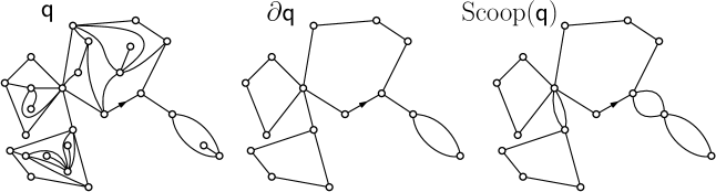
Figure 10: A rooted quadrangulation, its boundary and the associated scooped-out quadrangulation.

To a scooped-out quadrangulation we associate its tree of components $\operatorname{\textup{Tree}}(\operatorname{\textup{Scoop}}(\textup{$\mathsf{q}$}))$ as defined in Section 3.2.4. Following [23], we call this tree, by a slight abuse of terminology, the tree of components of $\mathsf{q}$ and use the notation $\mathsf{t}=\operatorname{\textup{{Tree}}}(\textup{$\mathsf{q}$})$. It is seen that vertices in $V(\mathsf{t}_{\bullet})$ have even degree in $\mathsf{t}$, due to the bipartite nature of $\mathsf{q}$.

By gluing the appropriate rooted quadrangulation with a simple boundary into each cycle of $\operatorname{\textup{Scoop}}(\textup{$\mathsf{q}$})$, we recover the quadrangulation $\mathsf{q}$. This provides a bijection

$$\Psi:\textup{$\mathsf{q}$}\mapsto(\operatorname{\textup{{Tree}}}(\textup{$\mathsf{q}$}),(\widehat{\textup{$\mathsf{q}$}}_{u}:u\in V(\operatorname{\textup{{Tree}}}(\textup{$\mathsf{q}$})_{\bullet}))$$

between, on the one hand, the set $\mathcal{Q}_{f}$ of finite rooted quadrangulations with a boundary and, on the other hand, the set of plane trees $\mathsf{t}$ with vertices at odd height having even degree, together with a collection $(\widehat{\textup{$\mathsf{q}$}}_{u}:u\in V(\mathsf{t}_{\bullet}))$ of rooted quadrangulations with a simple boundary and respective perimeter $\deg(u)$, for $\deg(u)$ the degree of $u$ in $\mathsf{t}$. We remark that the inverse mapping $\Psi^{-1}$ can be extended to an infinite but locally finite tree together with a collection of quadrangulations with a simple boundary attached to vertices at odd height, yielding in this case an infinite rooted quadrangulation $\mathsf{q}$.

Recall from Section 1.2.5 the definitions of the Boltzmann laws $\mathbb{P}_{g,z}$ and $\mathbb{P}_{g}^{\sigma}$, and their analogs with support on quadrangulations with a simple boundary, $\widehat{\mathbb{P}}_{g,z}$ and $\widehat{\mathbb{P}}_{g}^{\sigma}$. Their corresponding partition functions are $F$, $F_{\sigma}$ and $\widehat{F}$, $\widehat{F}_{\sigma}$. We are now interested in the law of the tree of components under $\mathbb{P}_{g,z}$. To begin with, we adapt some enumeration results from [15] to our setting. For every $0\leq p\leq 1/2$, recall that $g_{p}=p(1-p)/3$ and $z_{p}=(1-p)/4$. Then, (3.15), (3.27) and (5.16) of [15] all together provide the identities

$$F(g_{p},z_{p})=\frac{2}{3}\frac{3-4p}{1-p},\quad F_{\sigma}(g_{p})=\frac{(2\sigma)!}{\sigma!(\sigma+2)!}\left(2+\sigma\frac{1-2p}{1-p}\right)\left(\frac{1}{1-p}\right)^{\sigma},$$ (15)

for $0\leq p\leq 1/2$ and $\sigma\in\mathbb{N}_{0}$. Moreover, for $\sigma\in\mathbb{N}$ and $0<p\leq 1/2$,

$$\widehat{F}_{\sigma}(g_{p})=\left(\frac{p}{3(1-p)^{2}}\right)^{\sigma}\frac{(3\sigma-2)!}{\sigma!(2\sigma-1)!}\left(\frac{3\sigma(1-p)}{p}+2-3\sigma\right),$$ (16)

while $\widehat{F}_{0}(g_{p})=1$. If $p=0$ and hence $g_{p}=0$, then $\widehat{F}_{k}(0)=\delta_{0}(k)+\delta_{1}(k)$ for all $k\in\mathbb{N}_{0}$. (Indeed, under the maps with no inner faces, the vertex map and the map consisting of one oriented edge are the only maps with a simple boundary.)

We already introduced in Section 2.3 two probability measures $\mu_{\circ}$ and $\mu_{\bullet}$ on $\mathbb{N}_{0}$ given by

$$\mu_{\circ}(k) =\frac{1}{F(g_{p},z_{p})}\left(1-\frac{1}{F(g_{p},z_{p})}\right)^{k},\quad k\in\mathbb{N}_{0},$$ (17)

$$\mu_{\bullet}(2k+1) =\frac{1}{F(g_{p},z_{p})-1}\left[z_{p}F^{2}(g_{p},z_{p})\right]^{k+1}\widehat{F}_{k+1}(g_{p}),\quad k\in\mathbb{N}_{0},$$ (18)

with $\mu_{\bullet}(k)=0$ if $k$ even. The tree of components of the scooped-out quadrangulation $\operatorname{\textup{Scoop}}(Q)$ when $Q$ is drawn according to $\mathbb{P}_{g_{p},z_{p}}$ may now be characterized as follows.

Proposition 6.

Let $0\leq p\leq 1/2$, and let $Q$ be distributed according to $\mathbb{P}_{g_{p},z_{p}}$. Then the tree of components $\operatorname{\textup{{Tree}}}(Q)$ is a two-type Galton-Watson tree with offspring distribution $(\mu_{\circ},\mu_{\bullet})$ as given above. Moreover, conditionally on $\operatorname{\textup{{Tree}}}(Q)$, the quadrangulations with a simple boundary associated to $Q$ via the bijection $\Psi$ are independent with respective Boltzmann distribution $\widehat{\mathbb{P}}^{\deg(u)}_{g_{p}}$ for $u\in V(\operatorname{\textup{{Tree}}}(Q)_{\bullet})$, where $\deg(u)$ denotes the degree of $u$ in $\operatorname{\textup{{Tree}}}(Q)$.

Proof.

Note that vertices at even height of $\operatorname{\textup{{Tree}}}(Q)$ have an odd number of offspring almost surely. Let $\mathsf{t}$ be a finite plane tree satisfying this property. Let also $(\widehat{\textup{$\mathsf{q}$}}_{u}:u\in V(\mathsf{t}_{\bullet}))$ be a collection of rooted quadrangulations with a simple boundary and respective perimeters $\deg(u)$, and set $\textup{$\mathsf{q}$}=\Psi^{-1}(\mathsf{t},(\widehat{\textup{$\mathsf{q}$}}_{u}:u\in V(\mathsf{t}_{\bullet})))$. Then, writing $\Psi_{\ast}\mathbb{P}$ for the push-forward measure of $\mathbb{P}$ by $\Psi$,

$$\Psi_{\ast}\mathbb{P}_{g_{p},z_{p}}\left(\mathsf{t},(\widehat{\textup{$\mathsf{q}$}}_{u}:u\in V(\mathsf{t}_{\bullet}))\right)= \frac{z_{p}^{\#\partial\textup{$\mathsf{q}$}/2}g_{p}^{\#\textup{F}(\textup{$\mathsf{q}$})}}{F(g_{p},z_{p})}=\frac{1}{F(g_{p},z_{p})}\prod_{u\in V(\mathsf{t}_{\bullet})}z_{p}^{\deg(u)/2}g_{p}^{\#\textup{F}(\widehat{\textup{$\mathsf{q}$}}_{u})}.$$

For every $c>0$, we have

$$1=\prod_{u\in V(\mathsf{t}_{\circ})}{c^{k_{u}}\left(\frac{1}{c}\right)^{\#V(\mathsf{t}_{\bullet})}}\quad\text{and}\quad\frac{1}{c}=\prod_{u\in V(\mathsf{t}_{\bullet})}{c^{k_{u}}\left(\frac{1}{c}\right)^{\#V(\mathsf{t}_{\circ})}}.$$

Applying the first equality with $c=1-1/F(g_{p},z_{p})$ and the second one with $c=F(g_{p},z_{p})$ gives

$$\Psi_{\ast}\mathbb{P}_{g_{p},z_{p}}\left(\mathsf{t},(\widehat{\textup{$\mathsf{q}$}}_{u}:u\in V(\mathsf{t}_{\bullet})\right)=\prod_{u\in V(\mathsf{t}_{\circ})}{\frac{1}{F(g_{p},z_{p})}\left(1-\frac{1}{F(g_{p},z_{p})}\right)^{\deg(u)-1}}\\ \times\prod_{u\in V(\mathsf{t}_{\bullet})}{\frac{1}{F(g_{p},z_{p})-1}\left(z_{p}F^{2}(g_{p},z_{p})\right)^{\deg(u)/2}\widehat{F}_{\deg(u)/2}(g_{p})}\prod_{u\in V(\mathsf{t}_{\bullet})}{\frac{g_{p}^{\#\textup{F}(\widehat{\textup{$\mathsf{q}$}}_{u})}}{\widehat{F}_{\deg(u)/2}(g_{p})}},$$

where we agree that $0/0=0$. Therefore,

$$\Psi_{\ast}\mathbb{P}_{g_{p},z_{p}}\left(\mathsf{t},(\widehat{\textup{$\mathsf{q}$}}_{u}:u\in V(\mathsf{t}_{\bullet}))\right)=\prod_{u\in V(\mathsf{t}_{\circ})}{\mu_{\circ}(k_{u})}\prod_{u\in V(\mathsf{t}_{\bullet})}{\mu_{\bullet}(k_{u})}\prod_{u\in V(\mathsf{t}_{\bullet})}{\widehat{\mathbb{P}}^{\deg(u)}_{g_{p}}(\widehat{\textup{$\mathsf{q}$}}_{u})},$$

which is the expected result.∎

Corollary 4.

Let $0\leq p\leq 1/2$, $\sigma\in\mathbb{N}$, and let $Q$ be distributed according to $\mathbb{P}^{\sigma}_{g_{p}}$. Then the tree of components $\operatorname{\textup{{Tree}}}(Q)$ is a two-type Galton-Watson tree with offspring distribution $(\mu_{\circ},\mu_{\bullet})$ conditioned to have $2\sigma+1$ vertices. Moreover, conditionally on $\operatorname{\textup{{Tree}}}(Q)$, the quadrangulations with a simple boundary associated to $Q$ via the bijection $\Psi$ are independent with respective Boltzmann distribution $\widehat{\mathbb{P}}^{\deg(u)}_{g_{p}}$, for $u\in V(\operatorname{\textup{{Tree}}}(Q)_{\bullet})$.

Proof.

Observing that $\#V(\operatorname{\textup{{Tree}}}(\textup{$\mathsf{q}$}))=\#\partial\textup{$\mathsf{q}$}+1$ for every rooted quadrangulation $\mathsf{q}$, we obtain

$$\mathbb{P}_{g_{p},z_{p}}(\mathcal{Q}^{\sigma}_{f})=\Psi_{\ast}\mathbb{P}_{g_{p},z_{p}}\left(\{\mathsf{t}\in\mathbb{T}_{f}:\#V(\mathsf{t})=2\sigma+1\}\right)=\mathsf{GW}_{\mu_{\circ},\mu_{\bullet}}(\{\mathsf{t}\in\mathbb{T}_{f}:\#V(\mathsf{t})=2\sigma+1\}).$$

Now let $\mathsf{t}$ be a finite plane tree with an odd number of offspring at even height, and let $(\widehat{\textup{$\mathsf{q}$}}_{u}:u\in V(\mathsf{t}_{\bullet}))$ and $\mathsf{q}$ be as in the proof of Proposition 6. Then,

$$\Psi_{\ast}\mathbb{P}^{\sigma}_{g_{p}}\left(\mathsf{t},(\widehat{\textup{$\mathsf{q}$}}_{u}:u\in V(\mathsf{t}_{\bullet}))\right)=\frac{\mathbf{1}_{\{\#\partial\textup{$\mathsf{q}$}=2\sigma\}}}{\mathbb{P}_{g_{p},z_{p}}(\mathcal{Q}^{\sigma}_{f})}\prod_{u\in V(\mathsf{t}_{\circ})}{\mu_{\circ}(k_{u})}\prod_{u\in V(\mathsf{t}_{\bullet})}{\mu_{\bullet}(k_{u})}\prod_{u\in V(\mathsf{t}_{\bullet})}{\widehat{\mathbb{P}}^{\deg(u)}_{g_{p}}(\widehat{\textup{$\mathsf{q}$}}_{u})},$$

which concludes the proof.∎

Lemma 11.

For $0\leq p<1/2$, the pair $(\mu_{\circ},\mu_{\bullet})$ is critical and both $\mu_{\circ}$ and $\mu_{\bullet}$ have small exponential moments. For $p=1/2$, the pair $(\mu_{\circ},\mu_{\bullet})$ is subcritical (and $\mu_{\bullet}$ has no exponential moment).

Proof.

Recall that $(\mu_{\circ},\mu_{\bullet})$ is critical if and only if the product of their respective means $m_{\circ}$ and $m_{\bullet}$ equals one. Since by (17), $\mu_{\circ}$ is the geometric law with parameter $1/F(g_{p},z_{p})$, we have

$$m_{\circ}=F(g_{p},z_{p})-1.$$

For $m_{\bullet}$, we let $G_{\mu_{\bullet}}$ denote the generating function of $\mu_{\bullet}$. By (18), it follows that

$$G_{\mu_{\bullet}}(s)=\frac{1}{F(g_{p},z_{p})-1}\frac{1}{s}\left(\widehat{F}\left[g_{p},z_{p}F^{2}(g_{p},z_{p})s^{2}\right]-1\right),\quad s>0.$$

Then, Identity (2.8) of [15] ensures that $\widehat{F}(g,zF^{2}(g,z))=F(g,z)$ for all non-negative weights $g$ and $z$. When differentiating this relation with respect to the variable $z$, we obtain

$$\partial_{z}\widehat{F}(g,zF^{2}(g,z))=\frac{\partial_{z}F(g,z)}{F^{2}(g,z)+2zF(g,z)\partial_{z}F(g,z)}.$$ (19)

Writing

$$\partial_{z}F(g_{p},z_{p})=\sum_{\sigma\geq 0}\sigma F_{\sigma}(g_{p})z_{p}^{\sigma-1},$$

and using the exact expression for $F_{\sigma}(g_{p})$ from (15), we see by means of Stirling’s formula that $\partial_{z}F(g_{p},z_{p})=\infty$ for $p\in[0,1/2)$, and $\partial_{z}F(g_{p},z_{p})<\infty$ for $p=1/2$. Thus, for $p\in[0,1/2)$,

$$\partial_{z}\widehat{F}(g_{p},z_{p}F^{2}(g_{p},z_{p}))=\frac{1}{2z_{p}F(g_{p},z_{p})},$$

whereas if $p=1/2$, the derivative on the left-hand side in (19) is strictly smaller than the right-hand side for $g=g_{p}$, $z=z_{p}$. Finally, applying Identity (2.8) of [15] once again, we get

$$m_{\bullet}= G^{\prime}_{\mu_{\bullet}}(1)$$

$$= \frac{1}{F(g_{p},z_{p})-1}\left(-\left(\widehat{F}\left[g_{p},z_{p}F^{2}(g_{p},z_{p})\right]-1\right)+2z_{p}F^{2}(g_{p},z_{p})\partial_{z}\widehat{F}\left[g_{p},z_{p}F^{2}(g_{p},z_{p})\right]\right).$$

As a consequence, $m_{\circ}m_{\bullet}=1$ if $p<1/2$, and $m_{\circ}m_{\bullet}<1$ if $p=1/2$. The fact that $\mu_{\circ}$ has exponential moments is clear. For $\mu_{\bullet}$, one sees from (16) that the power series

$$\sum_{k\geq 0}x^{k}\widehat{F}_{k}(g_{p})$$

has radius of convergence $\widehat{r}_{p}=4(1-p)^{2}/(9p)$, while (15) ensures that

$$z_{p}F^{2}(g_{p},z_{p})=\frac{(1-4p)^{2}}{9(1-p)}.$$

Again, for $p\in[0,1/2)$, $\widehat{r}_{p}>z_{p}F^{2}(g_{p},z_{p})$, and these quantities are equal for $p=1/2$. Thus, there exists $s>1$ such that $G_{\mu_{\bullet}}(s)<\infty$ if and only if $p<1/2$, which concludes the proof.∎

We are now ready to prove Theorem 4.

Proof of Theorem 4.

Fix $0\leq p<1/2$. Let us denote by $\mathsf{Q}_{\infty}$ the random quadrangulation with an infinite boundary as constructed in the statement of Theorem 4, and let $Q_{\sigma}$ be distributed according to $\mathbb{P}^{\sigma}_{g_{p}}$. In view of Proposition 2, it is sufficient to prove that in the local sense, as $\sigma\rightarrow\infty$,

$$Q_{\sigma}\xrightarrow[]{(d)}\mathsf{Q}_{\infty}.$$ (20)

For every real $r\geq 1$ and every (finite or infinite) plane tree $\mathsf{t}$, we define $\operatorname{\textup{Cut}}_{r}(\mathsf{t})$ as the finite plane tree obtained from pruning all the vertices at a height larger than $2r$ in $\mathsf{t}$. If $\textup{$\mathsf{q}$}\in\mathcal{Q}$ is a quadrangulation with a boundary such that $\Psi(\textup{$\mathsf{q}$})=(\mathsf{t},(\widehat{\textup{$\mathsf{q}$}}_{u}:u\in V(\mathsf{t}_{\bullet})))$, we define $\operatorname{\textup{Cut}}_{r}(\textup{$\mathsf{q}$})$ to be the quadrangulation obtained from gluing the maps $(\widehat{\textup{$\mathsf{q}$}}_{u}:u\in V(\operatorname{\textup{Cut}}_{r}(\mathsf{t})_{\bullet}))$ in the associated loops of $\operatorname{\textup{Loop}}(\operatorname{\textup{Cut}}_{r}(\mathsf{t}))$. With this definition, we have $B_{r}(\textup{$\mathsf{q}$})\subset\operatorname{\textup{Cut}}_{r}(\textup{$\mathsf{q}$})$ for every $r\geq 1$, where we recall that $B_{r}(\textup{$\mathsf{q}$})$ stands for the closed ball of radius $r$ around the root in $\mathsf{q}$.

Let $r\geq 1$ and $\textup{$\mathsf{q}$}\in\mathcal{Q}_{f}$ such that $\Psi(\textup{$\mathsf{q}$})=(\mathsf{t},(\widehat{\textup{$\mathsf{q}$}}_{u}:u\in V(\mathsf{t}_{\bullet})))$. Using Proposition 6 and Corollary 4, we get

$$\mathbb{P}\left(\operatorname{\textup{Cut}}_{r}\left(Q_{\sigma}\right)=\textup{$\mathsf{q}$}\right)=\mathsf{GW}_{\mu_{\circ},\mu_{\bullet}}^{(2\sigma+1)}\left(\operatorname{\textup{Cut}}_{r}=\mathsf{t}\right)\prod_{u\in V(\mathsf{t}_{\bullet})}\widehat{\mathbb{P}}^{\deg(u)}_{g_{p}}\left(\widehat{\textup{$\mathsf{q}$}}_{u}\right),$$

where we use the notation $\mathsf{GW}_{\mu_{\circ},\mu_{\bullet}}^{(2\sigma+1)}$ for the $(\mu_{\circ},\mu_{\bullet})$-Galton-Watson tree conditioned to have $2\sigma+1$ vertices and interpret $\operatorname{\textup{Cut}}_{r}$ as the random variable $\mathsf{t}\mapsto\operatorname{\textup{Cut}}_{r}(\mathsf{t})$. Applying Proposition 3, we get as $\sigma\rightarrow\infty$

$$\mathbb{P}\left(\operatorname{\textup{Cut}}_{r}\left(Q_{\sigma}\right)=\textup{$\mathsf{q}$}\right)\longrightarrow\mathsf{GW}_{\mu_{\circ},\mu_{\bullet}}^{(\infty)}\left(\operatorname{\textup{Cut}}_{r}=\mathsf{t}\right)\prod_{u\in V(\mathsf{t}_{\bullet})}\widehat{\mathbb{P}}^{\deg(u)}_{g_{p}}\left(\widehat{\textup{$\mathsf{q}$}}_{u}\right)=\mathbb{P}\left(\operatorname{\textup{Cut}}_{r}\left(\mathsf{Q}_{\infty}\right)=\textup{$\mathsf{q}$}\right).$$

We proved that for every $r\geq 1$, as $\sigma\rightarrow\infty$,

$$\operatorname{\textup{Cut}}_{r}\left(Q_{\sigma}\right)\overset{(d)}{\longrightarrow}\operatorname{\textup{Cut}}_{r}\left(\mathsf{Q}_{\infty}\right).$$

Since $B_{r}(\textup{$\mathsf{q}$})\subset\operatorname{\textup{Cut}}_{r}(\textup{$\mathsf{q}$})$ for every $r\geq 1$ and $\textup{$\mathsf{q}$}\in\mathcal{Q}$, (20) holds and the theorem follows. ∎

6.2 Recurrence of simple random walk

In this final part, we prove Corollary 2, stating that simple random walk on the $\textup{{UIHPQ}}_{p}$ for $0\leq p<1/2$ is almost surely recurrent. We will use a criterion from the theory of electrical networks; see, e.g., [36, Chapter 2] for an introduction into these techniques.

Proof of Corollary 2.

Fix $0\leq p<1/2$. We interpret the $\textup{{UIHPQ}}_{p}$ as an electrical network, by equipping each edge with a resistance of strength one. A cutset $\mathcal{C}$ between the root vertex and infinity is a set of edges that separates the root from infinity, in the sense that every infinite self-avoiding path starting from the root has to pass through at least one edge of $\mathcal{C}$. By the criterion of Nash-Williams, cf. [36, (2.13)], it suffices to show that there is a collection $(\mathcal{C}_{n},n\in\mathbb{N})$ of disjoint cutsets such that $\sum_{n=1}^{\infty}(1/\#\mathcal{C}_{n})=\infty$ almost surely, i.e., for almost every realization of the $\textup{{UIHPQ}}_{p}$.

We recall the construction of the $\textup{{UIHPQ}}_{p}$ in terms of the looptree associated to Kesten’s two-type tree $\mathcal{T}_{\infty}=\mathcal{T}_{\infty}(\mu_{\circ},\mu_{\bullet})$. Note that the white vertices in $\mathcal{T}_{\infty}$, i.e., the vertices at even height, represent vertices in the $\textup{{UIHPQ}}_{p}$. More precisely, by construction, they form the boundary vertices of the latter. In particular, the white vertices on the spine of $\mathcal{T}_{\infty}$ are to be found in the $\textup{{UIHPQ}}_{p}$, and we enumerate them by $v_{1},v_{2},v_{3},\ldots$, such that $v_{1}$ is the root vertex, and $d_{\textup{gr}}(v_{j},v_{1})\geq d_{\textup{gr}}(v_{i},v_{1})$ for $j\geq i$. Now observe that for $i\in\mathbb{N}$, $v_{i}$ and $v_{i+1}$ lie on the boundary of one common finite-size quadrangulation with a simple boundary, which we denote by $\widehat{\textup{$\mathsf{q}$}}_{v_{i}}$, in accordance with notation in the proof of Theorem 4.

We define $\mathcal{C}_{i}$ to be the set of all the edges of $\widehat{\textup{$\mathsf{q}$}}_{v_{i}}$. Clearly, for each $i\in\mathbb{N}$, $\mathcal{C}_{i}$ is a cutset between the root vertex and infinity, and for $i\neq j$, $\mathcal{C}_{i}$ and $\mathcal{C}_{j}$ are disjoint. The sizes $\#\mathcal{C}_{i}$, $i\in\mathbb{N}$, are i.i.d. random variables. More specifically, using the construction of the $\textup{{UIHPQ}}_{p}$ in terms of Kesten’s looptree, the law of $\#\mathcal{C}_{1}$ can be described as follows: First, draw a random variable $Y$ according to the size-biased offspring distribution $\bar{\mu}_{\bullet}$, and then, conditionally on $Y$, $\#\mathcal{C}_{1}$ is distributed as the number of edges of a Boltzmann quadrangulation with law $\widehat{\mathbb{P}}_{g_{p}}^{(Y+1)/2}$, where $g_{p}=p(1-p)/3$. Obviously, $\#\mathcal{C}_{1}$ is finite almost surely, implying $\sum_{n=1}^{\infty}(1/\#\mathcal{C}_{n})=\infty$ almost surely, and recurrence of the simple symmetric random walk on the $\textup{{UIHPQ}}_{p}$ follows. ∎

Remark 11.

Let us end with a remark concerning the structure of the $\textup{{UIHPQ}}_{p}$ for $p<1/2$. Note that with probability $\bar{\mu}_{\bullet}(1)>0$, a cutset $\mathcal{C}_{i}$ as constructed in the above proof consists exactly of one edge. By independence and Borel-Cantelli, we thus find with probability one an infinite sequence of such cutsets $\mathcal{C}_{i_{1}},\mathcal{C}_{i_{2}},\ldots$ consisting of one edge only. In particular, this proves that the $\textup{{UIHPQ}}_{p}$ for $p<1/2$ admits a decomposition into a sequence of almost surely finite i.i.d. quadrangulations $Q_{i}(p)$ with a non-simple boundary (whose laws can explicitly be derived from Theorem 4), such that $Q_{i}(p)$ and $Q_{j}(p)$ get connected by a single edge if and only if $|i-j|=1$. This parallels the decomposition of the spaces $\mathbb{H}_{\alpha}$ for $\alpha<2/3$ found in [38, Display (2.3)].

Acknowledgments. We warmly thank Grégory Miermont for stimulating discussions and advice, and an anonymous referee for useful comments.

References

- [1] Abraham, C. Rescaled bipartite planar maps converge to the Brownian map. Ann. Inst. H. Poincaré Probab. Statist. 52(2) (2016), 575–595.
- [2] Aldous, D. The continuum random tree I. Ann. Probab. 19 (1991), 1–28.
- [3] Angel, O. Scaling of percolation on infinite planar maps, i. arXiv:0501006.
- [4] Angel, O., Curien, N. Percolation on random maps I: half-plane models. Ann. Inst. H. Poincaré Probab. Statist. 51(2) (2015), 405–431.
- [5] Angel, O., Ray, G. Classification of half-planar maps. Ann. Probab. 43(3) (2015), 1315–1349.
- [6] Angel, O., Ray, G. The half plane UIPT is recurrent. Probab. Theory Relat. Fields 170(3-4) (2018), 657–683.
- [7] Angel, O., Schramm, O. Uniform infinite planar triangulations. Comm. Math. Phys. 241(2-3) (2003), 191–213.
- [8] Baur, E., Miermont, G., Ray, G. Classification of scaling limits of uniform quadrangulations with a boundary. Ann. Probab. 6(47) (2019), 3397–3477.
- [9] Baur, E., Miermont, G., Richier, L. Geodesic rays in the Uniform Infinite Half-Planar Quadrangulation return to the boundary. Lat. Am. J. Probab. Math. Stat. 13 (2016), 1123–1149.
- [10] Benjamini, I., Schramm, O. Recurrence of distributional limits of finite planar graphs. Electron. J. Probab. 6(23) (2001), 13 pp.
- [11] Bettinelli, J. Scaling limit of random planar quadrangulations with a boundary. Ann. Inst. H. Poincaré 51(2) (2015), 432–477.
- [12] Bettinelli, J., Miermont, G. Compact Brownian surfaces I. Brownian disks. Probab. Theory Relat. Fields 167(3-4) (2017), 555–614.
- [13] Björnberg, J.E., Stefánsson, S. Ö. Recurrence of bipartite planar maps. Electron. J. Probab. 19(31) (2014), 1–40.
- [14] Bouttier, J., Di Francesco, P., Guitter, E. Planar maps as labeled mobiles. Electron. J. Combin. 11(1) (2004).
- [15] Bouttier, J., Guitter, E. Distance statistics in quadrangulations with a boundary, or with a self-avoiding loop. J. Phys. A. 42(46) (2009), 465208, 44 pp.
- [16] Budd, T. The Peeling Process of Infinite Boltzmann Planar Maps. Electron. J. Combin. 23(1), 1–28.
- [17] Budzinski, T. The hyperbolic Brownian plane. Probab. Theory Relat. Fields 167(1-2) (2018), 503–541.
- [18] Burago, D., Burago, I., Ivanov, S. A course in metric geometry. Graduate Studies in Mathematics (Book 33), AMS (2001).
- [19] Caraceni, A., Curien, N. Geometry of the uniform infinite half-planar quadrangulation. Random Struct. Algor. 52(3) (2018), 454–494.
- [20] Curien, N. Peeling random maps. Peccot lecture (2016) Available at http://www.math.u-psud.fr/curien/cours/peccot.pdf.
- [21] Curien, N. Planar stochastic hyperbolic triangulations. Probab. Theory Relat. Fields 165 (2016), 509–540.
- [22] Curien, N., Kortchemski, I. Random stable looptrees. Electron. J. Probab. 19(108) (2014), 35 pp.
- [23] Curien, N., Kortchemski, I. Percolation on random triangulations and stable looptrees. Probab. Theory Relat. Fields 163(1-2) (2015), 303–337.
- [24] Curien, N., Le Gall, J.-F. The Brownian plane. J. Theor. Probab. 27(4) (2014), 1249–1291.
- [25] Curien, N., Miermont, G. Uniform infinite planar quadrangulations with a boundary. Random Struct. Algor. 47(1) (2015), 30–58.
- [26] Gurel-Gurevich, O., Nachmias, A. Recurrence of planar graph limits. Ann. of Math. 177 (2013), 761–781.
- [27] Gwynne, E., Miller, J. Scaling limit of the uniform infinite half-plane quadrangulation in the Gromov-Hausdorff-Prokhorov-uniform topology. Electron. J. Probab. 22(84) (2017), 47 pp.
- [28] Ibragimov, I. A., Linnik, Ju V. Independent and stationary sequences of random variables. Wolters-Noordhoff Publishing, Groningen (1971).
- [29] Janson, S. Simply generated trees, conditioned Galton-Watson trees, random allocations and condensation. Probab. Surveys 9 (2012), 103–252.
- [30] Karatzas, I., Shreve, S. E. Brownian Motion and Stochastic Calculus. Graduate Texts in Mathematics (Book 113), Springer, 2nd edition (1991).
- [31] Kesten, H. Subdiffusive behavior of random walk on a random cluster. Ann. Inst. H. Poincaré Probab. Statist. 22(4) (1986), 425–487.
- [32] Krikun, M. Local structure of random quadrangulations. (2005), arXiv:0512304.
- [33] Le Gall, J.-F. Spatial branching processes, random snakes and partial differential equations. Lectures in Mathematics ETH Zürich. Birkhäuser, Basel (1999).
- [34] Le Gall, J.-F. Random trees and applications. Probability Surveys 2 (2005), 245–311.
- [35] Le Gall, J.-F., Miermont, G. Scaling Limits of Random Trees and Planar Maps. Clay Mathematics Proceedings 15 (2012).
- [36] Lyons, R., Peres, Y. Probability on trees and networks. Cambridge University Press, (2016).
- [37] Pitman, J. Combinatorial Stochastic Processes. École d’été de Probabilités de St. Flour. Lecture Notes in Mathematics 1875, Springer (2006).
- [38] Ray, G. Geometry and percolation on half planar triangulations. Electron. J. Probab. 19(47) (2014), 28 pp.
- [39] Richier, L. Universal aspects of critical percolation on random half-planar maps. Electron. J. Probab. 20 (2015), 45 pp.
- [40] Stephenson, R. Local convergence of large critical multi-type Galton-Watson trees and applications to random maps. J. Theor. Probab. 31(1) (2018), 159–205.