Performance Analysis and Compensation of Joint TX/RX I/Q Imbalance in Differential STBC-OFDM

Abstract

Differential space time block coding (STBC) achieves full spatial diversity and avoids channel estimation overhead. Over highly frequency-selective channels, STBC is integrated with orthogonal frequency division multiplexing (OFDM) to efficiently mitigate intersymbol interference effects. However, low-cost implementation of STBC-OFDM with direct-conversion transceivers is sensitive to In-phase/Quadrature-phase imbalance (IQI). In this paper, we quantify the performance impact of IQI at both the transmitter and receiver radio frequency front-ends on differential STBC-OFDM systems which has not been investigated before in the literature. In addition, we propose a widely-linear compensation algorithm at the receiver to mitigate the performance degradation caused by the IQI at the transmitter and receiver ends. Moreover, a parameter-based generalized algorithm is proposed to extract the IQI parameters and improve the performance under high-mobility. The adaptive compensation algorithms are blind and work in a decision-directed manner without using known pilots or training sequences. Numerical results show that our proposed compensation algorithms can effectively mitigate IQI in differential STBC-OFDM.

I Introduction

Space-time block-coded orthogonal frequency-division multiplexing (STBC-OFDM) is an effective transceiver structure to mitigate the wireless channel’s frequency selectivity while realizing multipaths and spatial diversity gains [1]. To acquire channel knowledge for signal detection at the receiver, STBC-OFDM schemes require the transmission of pilot signals [2]. However, to avoid the rate loss due to pilot signal overhead, we may want to forego channel estimation to avoid its complexity and the degradation of channel tracking quality in a fast time-varying environment [3, 4]. Differential transmission/detection, which is adopted in several standards such as digital audio broadcasting (DAB) [5], achieves this goal and has been successfully integrated with STBC-OFDM [2, 3, 6]. Although a differential STBC-OFDM system avoids the overhead of channel estimation, a low-cost transceiver implementation based on the direct-conversion architecture suffers from analog and radio-frequency (RF) impairments. The impairments in the analog components are mainly due to the uncontrollable fabrication process variations. Since most of these impairments cannot be effectively eliminated in the analog domain, an efficient compensation algorithm in the digital baseband domain would be highly desirable. One of the main sources of the analog impairments is the imbalance between the In-phase (I) and Quadrature-phase (Q) branches when the transmitted signal is up-converted to RF frequency at the transmitter, or the received RF signal is down-converted to baseband at the receiver. The I/Q imbalance (IQI) arises due to mismatches between the I and Q branches from the ideal case, $i.e.$, from the exact $90^{o}$ phase difference and equal amplitudes between the sine and cosine branches. In OFDM systems, IQI destroys the subcarrier orthogonality by introducing inter-carrier interference (ICI) between mirror subcarriers which can lead to serious performance degradation [7].

Many papers investigated IQI in single-input single-output OFDM systems (see [7, 8, 9, 10] and the references therein). There are also several works dealing with IQI in coherent multiple-antenna systems. In [11], a super-block structure for the Alamouti STBC scheme is designed to ensure orthogonality in the presence of IQI. In [12], an Expectation-Maximization-based algorithm is proposed to mitigate IQI in Alamouti-based STBC-OFDM systems. An equalization algorithm is proposed to mitigate IQI in STBC-OFDM systems in [13]. The authors in [14] analyze and compensate for IQI in single-carrier STBC systems. Precoding methods were investigated in coherent massive MIMO systems in [15]. In [16], I/Q imbalance effects were left uncompensated; instead, a link adaption strategy was considered and an IQI-aware transmission method was developed. In [17], an IQI-robust channel estimation and low-complexity compensation method for RX-IQI was proposed.

Although the compensation of IQI in STBC-OFDM systems has been well investigated, all of the existing works deal with IQI in a coherent system, where the channel state information (CSI) is assumed known or estimated at the receiver. To the best of our knowledge, there is no previous work dealing with joint transmitter and receiver IQI in differential transmission systems. Note that some blind or semi-blind estimation schemes that do not require CSI for IQI compensation have been proposed in the literature [18, 19, 20, 21]. A semi-blind compensation algorithm for IQI in MIMO-OFDM systems is presented in [18], where a blind signal separation (BSS) method is used to equalize the equivalent channel including IQI and the wireless multipath channel. However a known reference signal must be embedded in the transmitted signal. Another BSS-based IQI compensation method is presented in [19], and blind estimation methods of transmitter IQI (TX-IQI) and receiver IQI (RX-IQI) are presented in [20], [21]. The difference between the compensation algorithm in this paper and the blind compensation algorithms in [18, 19, 20, 21] is that blind compensation algorithms do not make use of the differential encoding property and they typically suffer from local optima and very slow convergence. On the other hand, although some of these blind compensation algorithms estimate IQI in a blind manner [19, 20, 21], they require equalization before the compensation of transmitter IQI, which is not feasible in a system with differential detection.

We extend the work in [22] which only analyzes and compensates for the effect of the RX-IQI in the differential STBC-OFDM (DSTBC-OFDM) transmission. In this paper, we analyze the joint impact of TX-IQI and RX-IQI in DSTBC-OFDM systems. An equivalent signal power degradation factor due to TX-IQI is derived. Moreover, by using the differential encoding property of the transmitted signal, we propose an adaptive decision-directed algorithm that uses a widely-linear (WL) structure to compensate for TX-IQI and RX-IQI without the need for knowing or estimating the CSI. Additionally, we propose a parameter-based (PB) generalized algorithm that can enhance the compensation performance under high-mobility. The rest of this paper is organized as follows: the system model of DSTBC-OFDM in the presence of TX-IQI and RX-IQI is developed in Section II. In Section III, we discuss the impact of IQI on the bit error rate (BER) performance of DSTBC-OFDM. We propose a decision-directed IQI compensation algorithm in Section IV and the numerical results are presented in Section V. Finally, we conclude our paper in Section VI.

Notations: Unless further noted, frequency-domain (FD) matrices and vectors are denoted by upper-case and lower-case boldface, respectively. Time-domain (TD) matrices and vectors are denoted by upper-case and lower-case boldface with under-bar, respectively. We denote the Hermitian, $i.e.$ complex-conjugate transpose of a matrix or a vector by ${{(\cdot)}^{H}}$. The conjugate and transpose of a matrix, a vector, or a scalar is denoted by ${{(\cdot)}^{*}}$ and ${{(\cdot)}^{T}}$, respectively. The symbol ${{[\mathbf{A}]}_{m,n}}$ denotes the entry at the $m$-th row and the $n$-th column of matrix $\mathbf{A}$. Matrix $\mathbf{F}$ is the $N$-point Discrete Fourier Transform (DFT) matrix whose entries are given by: ${{[\mathbf{F}]}_{m,n}}=\frac{1}{\sqrt{N}}\exp(-j\frac{2\pi}{N}mn)$, with $0\leq m,n\leq N-1$. $\textrm{Re}\{\cdot\}$ and $\textrm{Im}\{\cdot\}$ denote the real and imaginary parts of a complex number, respectively. For convenience, Table I summarizes the key variables used throughout the paper.

TABLE I: List of Key Variables

Var.	Definition
$N$	Number of subcarriers
$\rho_{t/r}$	Interference-to-signal ratio of TX/RX-IQI
$M$	Modulation order of PSK signal
$\mathbf{\Gamma}_{c}(n)$	Compensation matrix for the $n$-th subcarrier
$\mathbf{U}_{k}(n)$	$k$-th FD information block on the $n$-th subcarrier
$\lambda_{i}(n)$	FD channel of Subcarrier $n$ from the $i$-th transmit antenna
$\mathbf{S}_{k}\left(n\right)$	$k$-th FD STBC block on the $n$-th subcarrier
$g_{t/r}$	Amplitude imbalance of TX/RX
$\mathbf{\bar{S}}_{k}$	$k$-th FD STBC block on the $(N-n+2)$-th subcarrier
$\phi_{t/r}$	Phase imbalance of TX/RX

II System Model

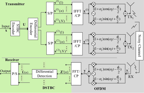
Figure 1: System model of DSTBC-OFDM under TX RX IQI

In this section, we briefly introduce the system model of DSTBC-OFDM under IQI depicted in Fig. 1. Without loss of generality, we consider an Alamouti-based [23] differential STBC-OFDM wireless communication system equipped with two transmit antennas and a single receive antenna. For a multiple-antenna receiver, the analysis and compensation algorithms in this paper can also be straightforwardly applied. Since OFDM transmission divides the channel into $N$ mutually orthogonal subcarriers, the OFDM-STBC input-output model at the $n$-th subcarrier can be expressed as follows [3]

$$\mathbf{z}_{k}(n) = \left[\begin{matrix}\lambda_{1}(n)&\lambda_{2}(n)\end{matrix}\right]\underset{\mathbf{S}_{k}\left(n\right)}{\underbrace{\left[\begin{array}[]{cc}s_{1}(k,n)&s_{2}(k,n)\\ -s_{2}^{*}(k,n)&s_{1}^{*}(k,n)\end{array}\right]}}$$ (5)

$$+\left[\begin{array}[]{cc}v_{2k+1}(n)&v_{2k+2}(n)\end{array}\right],$$

where $\mathbf{z}_{k}(n)=\left[\begin{array}[]{cc}z_{2k+1}(n)&z_{2k+2}(n)\end{array}\right]$ is the received vector corresponding to the $(2k+1)$-th and $(2k+2)$-th received OFDM symbols, respectively. Moreover, the matrix $\mathbf{S}_{k}\left(n\right)$ is the $k$-th frequency-domain differentially-encoded STBC transmission matrix at the $n$-th subcarrier, whose first and second columns are transmitted over the $(2k-1)$-th and $2k$-th OFDM symbols, respectively. The first and second rows of $\mathbf{S}_{k}\left(n\right)$ are transmitted by the first and second transmit antennas, respectively. In addition, $v_{2k+1}(n)$ and $v_{2k+1}(n)$ are the frequency-domain additive noise symbols at the $n$-th subcarrier. The scalars $\lambda_{i}(n)$ ($i=1,2$) correspond to the channel coefficients between the $i$-th transmit antenna and the single receive antenna at the $n$-th subcarrier where the vector $\boldsymbol{\lambda}_{i}=[\lambda_{i}(1),\lambda_{i}(2),...,\lambda_{i}(N)]$ is given by [7]

$$\boldsymbol{\lambda}_{i}=\sqrt{N}\mathbf{F}^{H}\left[\begin{matrix}\mbox{ }\mathbf{\underline{h}}_{i}\\ \mathbf{0}_{\left(N-\left(L+1\right)\right)\times 1}\end{matrix}\right],$$ (6)

and the vector $\mbox{ }\mathbf{\underline{h}}_{i}=\left[\underline{h}_{0}^{\left(i\right)}\,\underline{h}_{1}^{\left(i\right)}\,\cdots\,\underline{h}_{L}^{\left(i\right)}\right]^{T}$ is the time-domain channel impulse response (CIR) vector between the $i$-th transmit antenna and the single receive antenna with $L+1$ independent taps.

The differential encoding rule used to generate $\mathbf{S}_{k}\left(n\right)$ in Eq. (5) is given by [3]

$$\mathbf{S}_{k+1}(n)=\mathbf{S}_{k}(n)\mathbf{U}_{k+1}(n),$$ (7)

where $\mathbf{U}_{k+1}(n)$ is a $2\times 2$ Alamouti-structured information matrix given by

$$\mathbf{U}_{k+1}(n)=\left[\begin{array}[]{cc}u_{1}(k+1,n)&u_{2}(k+1,n)\\ -u_{2}^{*}(k+1,n)&u_{1}^{*}(k+1,n)\end{array}\right],$$ (8)

where the symbols $u_{1}(k+1,n)$ and $u_{2}(k+1,n)$ are drawn from a constant-modulus signal constellation $\varPsi$ (usually M-ary phase shift keying (M-PSK) symbols), which is required by a conventional differential transceiver. Note that few researchers have investigated using a non-constant-modulus signal constellation in a differential transceiver[24][25], where further operations are needed to extract the amplitude information at the receiver which is beyond the scope of this paper. Using the same approach followed in [3], Eq. (5) can be expressed in the form of $\mathbf{Z}_{k}\left(n\right)=\mathbf{\Lambda}\left(n\right)\mathbf{S}_{k}\left(n\right)+\mathbf{V}_{k}\left(n\right)$ as follows

$${\small\begin{array}[]{c}{{\bf{Z}}_{k}}\left(n\right)=\underbrace{\left[{\begin{array}[]{*{20}{c}}{{\lambda_{1}}(n)}&{{\lambda_{2}}(n)}\\ {-\lambda_{2}^{*}(n)}&{\lambda_{1}^{*}(n)}\end{array}}\right]}_{{\bf{\Lambda}}\left(n\right)}\underbrace{\left[{\begin{array}[]{*{20}{c}}{{s_{1}}(k,n)}&{{s_{2}}(k,n)}\\ {-s_{2}^{*}(k,n)}&{s_{1}^{*}(k,n)}\end{array}}\right]}_{{{\bf{S}}_{k}}\left(n\right)}\\ +\underbrace{\left[{\begin{array}[]{*{20}{c}}{{v_{2k+1}}(n)}&{{v_{2k+2}}(n)}\\ {-v_{2k+2}^{*}(n)}&{v_{2k+1}^{*}(n)}\end{array}}\right]}_{{{\bf{V}}_{k}}\left(n\right)}\end{array}}$$ (9)

where $\bf{Z}_{k}$ is also an Alamouti matrix given by

$${{\bf{Z}}_{k}}\left(n\right)=\left[{\begin{array}[]{*{20}{c}}{{z_{2k+1}}(n)}&{{z_{2k+2}}(n)}\\ {-z_{2k+2}^{*}(n)}&{z_{2k+1}^{*}(n)}\end{array}}\right].$$ (10)

Based on the STBC-OFDM model in Eq. (9) and the differential encoding in Eq. (7), the received signal blocks $\mathbf{Z}_{k}\left(n\right)$ and $\mathbf{Z}_{k+1}\left(n\right)$ are defined by

$$\mathbf{Z}_{k}\left(n\right) =\mathbf{\Lambda}(n)\mathbf{S}_{k}\left(n\right)+\mathbf{V}_{k}\left(n\right),$$

$$\mathbf{Z}_{k+1}\left(n\right) =\mathbf{\Lambda}(n)\mathbf{S}_{k+1}\left(n\right)+\mathbf{V}_{k+1}\left(n\right)$$

$$=\mathbf{\Lambda}(n)\mathbf{S}_{k}(n)\mathbf{U}_{k+1}(n)+\mathbf{V}_{k+1}\left(n\right).$$ (11)

Therefore, the maximum likelihood (ML) decoder for the information matrix $\mathbf{U}_{k+1}(n)$ is given by [6]

$$\mathbf{\hat{U}}_{k+1}(n)=\underset{\mathbf{\quad\quad\quad\mathbf{U}}}{\mathop{\arg}\quad\mathop{\max}}\,\left\{\mathbf{\mathbf{U}}^{H}\mathbf{Z}_{k}^{H}\left(n\right)\mathbf{Z}_{k+1}\left(n\right)\right\},$$ (12)

where $\mathbf{\mathbf{U}}$ is chosen from the Alamouti matrix sets formed by all possible information matrices.

Starting from the system model in Eqs. (9) and (11), we adopt the time-domain TX-IQI and RX-IQI model defined in [7]. For a given generalized time-domain baseband signal $\underline{b}\left(t\right)$, the signals that are distorted by the TX-IQI and RX-IQI, denoted by $\underline{b}_{t}^{\prime}\left(t\right)$ and $\underline{b}_{r}^{\prime}\left(t\right)$, respectively, can be expressed as follows

$$\underline{b}_{t}^{\prime}\left(t\right)=\alpha_{t}\underline{b}\left(t\right)+\beta_{t}\underline{b}^{*}\left(t\right), \underline{b}_{r}^{\prime}\left(t\right)=\alpha_{r}\underline{b}\left(t\right)+\beta_{r}\underline{b}^{*}\left(t\right).$$ (13)

The parameters $(\alpha_{t},\beta_{t})$ and $(a_{r},\beta_{r})$ are the TX-IQI and RX-IQI parameters, respectively, which are defined by

$$\alpha_{t}=\cos(\frac{\phi_{t}}{2})+jg_{t}\sin(\frac{\phi_{t}}{2}),\thinspace\beta_{t}=g_{t}\cos(\frac{\phi_{t}}{2})-j\sin(\frac{\phi_{t}}{2}),$$

$$\alpha_{r}=\cos(\frac{\phi_{r}}{2})+jg_{r}\sin(\frac{\phi_{r}}{2}),\thinspace\beta_{r}=g_{r}\cos(\frac{\phi_{r}}{2})-j\sin(\frac{\phi_{r}}{2}),$$ (14)

where $g_{t}$, $\phi_{t}$ and $g_{r}$, $\phi_{r}$ are the amplitude and the phase imbalance between the I and Q branches in the transmitter and receiver ends, respectively. The transmit and receive amplitude imbalances are often denoted in dB as $10\log(1+g_{t})$ and $10\log(1+g_{r})$, respectively [7]. The overall imbalance of a transceiver is measured by the Image Rejection Ratio (IRR), which is defined by $\mbox{IRR}_{t}(dB)\triangleq-10\log_{10}(\rho_{t})=-10\log_{10}(|{{\beta}_{t}}|^{2}/|{{\alpha}_{t}}|^{2})=-20\log_{10}(|{{\beta}_{t}}|/|{{\alpha}_{t}}|)$ and $\mbox{IRR}_{r}(dB)\triangleq-10\log_{10}(\rho_{r})=-20\log_{10}(|{{\beta}_{r}}|/|{{\alpha}_{r}}|)$, where $\rho_{t}$ and $\rho_{r}$ could be equivalently viewed as the normalized interference powers introduced by TX-IQI and RX-IQI, respectively.

In an OFDM system, discarding the samples corresponding to the $1^{st}$ and $\left(\frac{N}{2}+1\right)$-th subcarriers, the effect of the IQI on the $n$-th subcarrier of the DSTBC-OFDM received signal is basically introducing ICI from its $\left(N-n+2\right)$-th image subcarrier [8]. Based on the DSTBC-OFDM model in Eq. (11), the frequency-domain received signal blocks $\mathbf{Z^{\prime}}_{k}\left(n\right)$ and $\mathbf{Z^{\prime}}_{k+1}\left(n\right)$, which are jointly distorted by TX-IQI and RX-IQI, are given by

$$\mathbf{\mathbf{Z^{\prime}}}_{k}\left(n\right) = \left(\mathbf{A}_{t}\mathbf{A}_{r}\mathbf{\Lambda}(n)+\mathbf{B}_{t}^{*}\mathbf{B}_{r}\bar{\Lambda}(n)\right)\mathbf{S}_{k}\left(n\right)$$ (15)

$$+\left(\mathbf{A}_{r}\mathbf{B}_{t}\mathbf{\Lambda}(n)+\mathbf{A}_{t}^{*}\mathbf{B}_{r}\mathbf{\bar{\Lambda}}(n)\right)\mathbf{\bar{S}}_{k}\left(n\right)$$

$$+\mathbf{A}_{r}\mathbf{V}_{k}\left(n\right)+\mathbf{B}_{r}\mathbf{\bar{V}}_{k}\left(n\right),$$

$$\mathbf{\mathbf{Z^{\prime}}}_{k+1}\left(n\right) = \left(\mathbf{A}_{t}\mathbf{A}_{r}\mathbf{\Lambda}(n)+\mathbf{B}_{t}^{*}\mathbf{B}_{r}\bar{\Lambda}(n)\right)\mathbf{S}_{k+1}\left(n\right)$$ (16)

$$+\left(\mathbf{A}_{r}\mathbf{B}_{t}\mathbf{\Lambda}(n)+\mathbf{A}_{t}^{*}\mathbf{B}_{r}\mathbf{\bar{\Lambda}}(n)\right)\mathbf{\bar{S}}_{k+1}\left(n\right)$$

$$+\mathbf{A}_{r}\mathbf{V}_{k+1}\left(n\right)+\mathbf{B}_{r}\mathbf{\bar{V}}_{k+1}\left(n\right)$$

$$= \left(\mathbf{A}_{t}\mathbf{A}_{r}\mathbf{\Lambda}(n)+\mathbf{B}_{t}^{*}\mathbf{B}_{r}\bar{\Lambda}(n)\right)\mathbf{S}_{k}(n)\mathbf{U}_{k+1}(n)$$

$$+\left(\mathbf{A}_{r}\mathbf{B}_{t}\mathbf{\Lambda}(n)+\mathbf{A}_{t}^{*}\mathbf{B}_{r}\mathbf{\bar{\Lambda}}(n)\right)\mathbf{\bar{S}}_{k}(n)\mathbf{\bar{U}}_{k+1}(n)$$

$$+\mathbf{A}_{r}\mathbf{V}_{k+1}\left(n\right)+\mathbf{B}_{r}\mathbf{\bar{V}}_{k+1}\left(n\right),$$

where $\mathbf{\bar{\Lambda}}(n)=\mathbf{\Lambda}^{*}(N-n+2)$, $\mathbf{\bar{V}}_{k}\left(n\right)=\mathbf{V}_{k}^{*}\left(N-n+2\right)$, $\mathbf{\bar{V}}_{k+1}\left(n\right)=\mathbf{V}_{k+1}^{*}\left(N-n+2\right)$, $\mathbf{\bar{U}}_{k+1}(n)=\mathbf{U}_{k+1}^{*}(N-n+2)$ and $\mathbf{\bar{S}}_{k+1}(n)=\mathbf{\bar{S}}_{k}(n)\mathbf{\bar{U}}_{k+1}(n)=\mathbf{S}_{k+1}^{*}\left(N-n+2\right)$. Moreover, the matrices $\mathbf{A}_{t/r}$, $\mathbf{B}_{t/r}$ are constructed from the IQI parameters as follows

$$\mathbf{A}_{t/r} =\left[\begin{matrix}\alpha_{t/r}&0\\ 0&\alpha_{t/r}^{*}\end{matrix}\right],\;\;\mathbf{B}_{t/r}=\left[\begin{matrix}\beta_{t/r}&0\\ 0&\beta_{t/r}^{*}\end{matrix}\right].$$ (17)

III Performance Analysis of DSTBC-OFDM under I/Q Imbalance

In this section, we first analyze the impact of TX-IQI and RX-IQI separately on an individual subcarrier in DSTBC-OFDM with M-PSK signaling, and then present the combined effect of TX-IQI and RX IQI on the BER performance. For notation simplicity, we omit the subcarrier index $n$. In addition, recall that the entries of differentially-encoded matrices, ${{\mathbf{S}}_{k}}$ and $\mathbf{{\mathbf{\bar{S}}}}_{k}$, are sums of numerous products of PSK symbols, for a long input data sequence, we apply the central limit theorem (CLT) to approximate the distributions of the entries of ${{\mathbf{S}}_{k}}$, $\mathbf{S}_{k}^{H}\mathbf{\bar{S}}_{k+1}$ and $\mathbf{\bar{S}}_{k}^{H}\mathbf{S}_{k+1}$ by the uncorrelated zero-mean Gaussian distributions ${{\mathbf{S}}_{k}}\sim\mathcal{N}\left(0,\,\frac{1}{2}\right)$, $\mathbf{S}_{k}^{H}\mathbf{\bar{S}}_{k+1}\sim\mathcal{N}\left(0,\,\frac{1}{2}\right)$ and $\mathbf{\bar{S}}_{k}^{H}\mathbf{S}_{k+1}\sim N\left(0,\,\frac{1}{2}\right)$ with a variance of $\frac{1}{2}$ to satisfy the power constraint $\mathbf{S}_{k}\mathbf{S}_{k}^{H}=\mathbf{S}_{k}^{H}\mathbf{\bar{S}}_{k+1}\left(\mathbf{S}_{k}^{H}\mathbf{\bar{S}}_{k+1}\right)^{H}=\mathbf{\bar{S}}_{k}^{H}\mathbf{S}_{k+1}\left(\mathbf{\bar{S}}_{k}^{H}\mathbf{S}_{k+1}\right)^{H}=\mathbf{I}$.

On the other hand, after discarding the samples corresponding to the $1^{st}$ and $\left(\frac{N}{2}+1\right)$-th subcarriers, we assume that both the STBC block $\mathbf{S}_{k}^{H}(n)$ and the frequency-domain channel response $\Lambda(n)$ of the desired subcarrier are independent of their counterparts of the image subcarrier, namely, $\mathbf{\mathbf{\bar{S}}}_{k}^{H}(n)$ and $\bar{\Lambda}(n)$, respectively [26].

To further simplify the notation, note that according to Eqs. (15) and (16), in the presence of TX-IQI, for each OFDM symbol, the equivalent transmitted signal $s^{\prime}(k,n)=\alpha_{t}s(k,n)+\beta_{t}s^{*}\left(k,N-n+2\right)$ is a linear combination of two independent Gaussian random variables whose phases are uniformly distributed. Thus, we can replace the IQI parameters $\alpha_{t}$ and $\beta_{t}$ with their absolute values $|\alpha_{t}|$ and $|\beta_{t}|$, respectively, in our following performance analysis without changing the received signal statistical properties. Similarly, from Eq. (6), the diagonal entries of matrix $\mathbf{\Lambda}$ correspond to the DFT of the multi-path CIR whose $L+1$ coefficients follow a zero-mean Gaussian distribution. Thus, the non-zero entries of the diagonal matrix $\mathbf{\Lambda}$ follow a zero-mean Gaussian distribution with unit variance [27]. Hence, the received signal also has a uniformly-distributed phase, and we can also replace the RX-IQI parameters $\alpha_{r}$ and $\beta_{r}$ with their absolute values $|\alpha_{r}|$ and $|\beta_{r}|$ in our following performance analysis. Thus, the IQI diagonal matrices $\mathbf{A}_{t}$, $\mathbf{B}_{t}$, $\mathbf{A}_{r}$ and $\mathbf{B}_{r}$ become $\mathbf{A}_{t/r}=\left|\alpha_{t/r}\right|\mathbf{I}$ and $\mathbf{B}_{t/r}=\left|\beta_{t/r}\right|\mathbf{I}$, respectively. The accuracy of these assumptions is also supported by the analysis of IQI in OFDM systems in [26], [28], where the impact of the IQI depends only on $\left|\alpha_{t/r}\right|$ and $\left|\beta_{t/r}\right|$.

For the following subsections, we quantify the asymptotic BER floor caused by TX-IQI and RX-IQI and its corresponding equivalent signal-to-noise ratio (SNR) compared to that of the IQI-free system. We also compare the impact of IQI in differential and coherent STBC-OFDM.

III-A DSTBC-OFDM under TX-IQI only

Based on the previous assumptions, the frequency-domain received signals $\mathbf{\mathbf{Z^{\prime}}}_{k}\left(n\right)$ and $\mathbf{\mathbf{Z^{\prime}}}_{k+1}\left(n\right)$ in Eq. (15) and Eq. (16), in the presence of only TX-IQI can be expressed as

$$\begin{array}[]{cl}\mathbf{\mathbf{Z^{\prime}}}_{TX,k}&=|{{a}_{t}}|\mathbf{\Lambda}\mathbf{S}_{k}+|{{\beta}_{t}}|\mathbf{\Lambda}\mathbf{\bar{S}}_{k}+\mathbf{V}_{k},\\ \mathbf{\mathbf{Z^{\prime}}}_{TX,k+1}&=|{{a}_{t}}|\mathbf{\Lambda}\mathbf{S}_{k+1}+|{{\beta}_{t}}|\mathbf{\Lambda}\mathbf{\bar{S}}_{k+1}+\mathbf{V}_{k+1}\\ &=|{{a}_{t}}|\mathbf{\Lambda}\mathbf{S}_{k}\mathbf{U}_{k+1}+|{{\beta}_{t}}|\mathbf{\Lambda}\mathbf{\bar{S}}_{k}\mathbf{\bar{U}}_{k+1}+\mathbf{V}_{k+1},\end{array}$$ (18)

From Eq. (12), the decoding metric for the ML decoder under TX-IQI is given by

$$\mathbf{\mathbf{Z^{\prime}}}_{TX,k}^{H}\mathbf{\mathbf{Z^{\prime}}}_{TX,k+1} =|\lambda|^{2}|a_{t}|^{2}\mathbf{U}_{k+1}+\mathbf{V}_{TX}$$ (19)

$$+|\lambda|^{2}\underset{\Theta_{TX}}{\underbrace{|\alpha_{t}\beta_{t}|\mathbf{S}_{k}^{H}\mathbf{\mathbf{\bar{S}}}_{k+1}+|\alpha_{t}\beta_{t}|\mathbf{\bar{S}}_{k}^{H}\mathbf{\mathbf{S}}_{k+1}}},$$

where $\mathbf{V}_{TX}=|\alpha_{t}|\mathbf{V}_{k}^{H}\mathbf{\Lambda\mathbf{S}}_{k}\mathbf{U}_{k+1}+|\alpha_{t}|\mathbf{S}_{k}^{H}\mathbf{\Lambda}^{H}\mathbf{V}_{k+1}$, $|\lambda|^{2}\mathbf{I}=\mathbf{\Lambda}^{H}\mathbf{\Lambda}=(|\lambda_{1}^{2}(n)|+|\lambda_{2}^{2}(n)|)\mathbf{I}$. Eq. (19) shows that TX-IQI will distort the transmitted signal by introducing a Gaussian error term to the transmitted signal.

For a given channel realization at the desired subcarrier, the instantaneous BER of the M-PSK symbols in $\mathbf{U}_{k+1}$ is determined by the instantaneous equivalent signal-to-interference-plus-noise ratio (SINR) of $\mathbf{U}_{k+1}$ in the decoding metric [27]. Thus, we derive the average BER of DSTBC-OFDM by averaging the conditional instantaneous BER over the probability distribution function (PDF) of the equivalent SINR.

Asymptotically, it can be proved that when IRR is higher than a certain level, TX-IQI will not cause any error floor when $\mathrm{SNR}\rightarrow\infty$ ($i.e.$ ${{\sigma}^{2}}\rightarrow 0$) due to the power constraint on $\Theta_{TX}$. More specifically, let $A_{min}$ be the minimum power of the error term that will cause an error in the detection of the M-PSK constellation symbols. TX-IQI will not lead to a non-zero asymptotic BER ($i.e.$ error floor) as $\mathrm{SNR}\rightarrow\infty$ unless $|\beta_{t}|/|\alpha_{t}|=\sqrt{\rho_{t}}<\sqrt{2}A_{min}/4$ (see Appendix A for proof). For a normalized QPSK signal with hard detection, it is easy to calculate that $A_{min,QPSK}=1/\sqrt{2}$, which means that if $\mbox{IRR}_{t}(dB)=20\log(|{{\alpha}_{t}}|/|{{\beta}_{t}}|)$ is larger than $12.04$dB, there will no error floor for a DSTBC-OFDM system using a QPSK constellation under TX-IQI as $\mathrm{SNR}\rightarrow\infty$. For 8-PSK constellation, we have $A_{\min}=0.3827$, which means that a BER floor appears only when IRR is smaller than $17.4$dB.

First, we derive the asymptotic BER when $\mathrm{SNR}\rightarrow\infty$ (BER floor) under severe TX-IQI, $i.e.$ $\mbox{IRR}_{t}(dB)<12.04(dB)$ for QPSK and $\mbox{IRR}_{t}(dB)<17.4(dB)$ for 8-PSK. In these cases, since ${{\mathbf{S}}_{k}}^{H}\mathbf{{\mathbf{\bar{S}}}}_{k+1}$ and ${{\mathbf{\bar{S}}}_{k}}^{H}\mathbf{{\mathbf{S}}}_{k+1}$ are independent Gaussian matrices, the detection metric in Eq. (19) is given by

$$\mathbf{\mathbf{Z^{\prime}}}_{TX,k}^{H}\mathbf{\mathbf{Z^{\prime}}}_{TX,k+1}=|\lambda|^{2}\left(|{{a}_{t}}|^{2}\mathbf{U}_{k+1}+\Theta_{TX}\right),$$ (20)

which is equivalent to transmitting a PSK symbol matrix $\mathbf{U}_{k+1}$ over an AWGN channel. Moreover, based on the assumed independence between the desired subcarriers and their image subcarriers, $i.e.$ $E\{\mathbf{S}_{k}^{H}\mathbf{{\mathbf{\bar{S}}}}_{k+1}\mathbf{{\mathbf{S}}}_{k+1}^{H}{{\mathbf{\bar{S}}}_{k}}\}=0$, each entry in $\Theta_{TX}$ is a zero-mean Gaussian random variable whose variance is given by

$${{E}_{\Theta,TX}}=\frac{1}{4}E\{Tr({{\Theta_{TX}}^{H}}\Theta_{TX})\}=|{{\alpha}_{t}}{{\beta}_{t}}{{|}^{2}}.$$ (21)

The asymptotic instantaneous SINR ($i.e.$ ${{\sigma}^{2}}\rightarrow 0$) of the equivalent system in Eq. (20) is

$$\eta_{TX}^{(a)} = Tr\{|a_{t}|^{4}\mathbf{U}_{k+1}^{H}\mathbf{U}_{k+1}\}/E\left\{Tr\left(\Theta_{TX}^{H}\Theta_{TX}\right)\right\}$$ (22)

$$= \frac{|a_{t}|^{2}}{2|\beta_{t}|^{2}}=\frac{\rho_{t}^{-1}}{2}.$$

Based on the general relationship between the BER and the instantaneous SINR, denoted by $\eta_{t}^{(a)}$, of an M-PSK signal in [27], the asymptotic BER (error floor) under severe TX-IQI, denoted by $P_{e,TX}^{(a)}$, is given by

$$P_{e,Tx}^{(a)} =\frac{1}{\log_{2}M}erfc\left(\sqrt{\eta_{t}^{(a)}}\sin\left(\pi/M\right)\right)$$ (23)

$$=\frac{1}{\log_{2}M}erfc\left(\sqrt{\frac{\rho_{t}^{-1}}{2}}\sin\left(\pi/M\right)\right).$$

The BER floor given in Eq. (23) will only occur under severe TX-IQI, which is $\mbox{IRR}_{t}(dB)<12.04(dB)$ for QPSK and ${\mbox{IRR}_{t}(dB)<17.4(dB)}$ for 8-PSK. In other situations, there will be no BER floor caused by TX-IQI and we will derive an equivalent SINR loss in these situations. Since the detection of symbols in $\mathbf{U}_{k+1}$ is totally determined by the detection metric in Eq. (19), the transmitted signal $\mathbf{U}_{k+1}$ could be viewed as being distorted by the error vector $\Theta_{TX}=|{{\alpha}_{t}}{{\beta}_{t}}|{{\mathbf{S}}_{k}^{H}}\mathbf{{\mathbf{\bar{S}}}}_{k+1}+|{{\alpha}_{t}}{{\beta}_{t}}|{{\mathbf{\bar{S}}}_{k}^{H}}\mathbf{{\mathbf{S}}}_{k+1}$. Based on the independence between the desired and image OFDM subcarriers, each entry in $\Theta_{TX}$ is a zero-mean Gaussian random variable whose variance is $|\alpha_{t}\beta_{t}|^{2}$ as given by Eq. (21).

Hence, to simplify the analysis, as depicted in Fig. 2, the PSK symbols in $\mathbf{U}_{k+1}$ can be viewed as being distorted by a zero-mean complex Gaussian random vector $|\alpha_{t}\beta_{t}|n^{\prime}$, where $n^{\prime}$ is a standard Gaussian random variable, $i.e.$ $E\{n^{\prime}\}=0$ and $E\{|n^{\prime}|^{2}\}=1$. The distance between the distorted symbol $u^{\prime}=u+n^{\prime}$ and the PSK decision boundaries ($\overline{OA}$ and $\overline{OB}$ in Fig. 2), denoted as $D(u^{\prime},\overline{OA})$ and $D(u^{\prime},\overline{OB})$ , respectively, are changed by $n^{\prime}$, which equivalently results in an amplitude loss $\varepsilon^{\prime}$ in the signal amplitude. Further details can be found in Appendix B. According to the analysis in Appendix B, the equivalent transmitted signal power under the disturbance of $n^{\prime}$ is given by

$$E_{s,TX}=|\alpha_{t}|^{4}(1+\sqrt{1+\cot(\pi/M)^{2}}\sqrt{|\rho_{t}|}n^{\prime})^{2}/2.$$ (24)

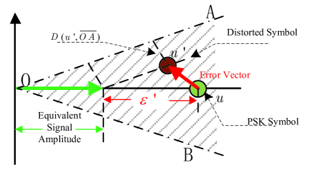
Figure 2: Equivalent signal amplitude in the presence of TX-IQI

Clearly, the transmitted signal amplitude is affected by a zero-mean random variable. Since the BER is determined by the tail of the error function, the random variation in the transmitted signal power causes more errors. To model the BER increase, we define the equivalent signal amplitude loss due to TX-IQI as $\varepsilon_{TX}$. Since the BER of M-PSK is approximately proportional to the inverse of the square of the transmitted signal power [27], thus $\varepsilon_{TX}$ is chosen to fit the expectation of the inverse of the square of the transmitted power. Hence, using Eq. (24), we have

$$E\left(\frac{1}{E_{s,TX}^{2}}\right)=\frac{4}{|a_{t}|^{8}}E\left(\frac{1}{(1+\sqrt{1+\cot(\pi/M)^{2}}\sqrt{\rho_{t}}n^{\prime})^{4}}\right).$$ (25)

Thus, the equivalent amplitude loss $\varepsilon_{TX}$ should be chosen to satisfy the following equation

$$\frac{4}{|a_{t}|^{8}(1-\varepsilon_{TX})^{4}}=\frac{4}{|a_{t}|^{8}}E\left(\frac{1}{(1+\sqrt{1+\cot(\pi/M)^{2}}\sqrt{\rho_{t}}n^{\prime})^{4}}\right).$$ (26)

The factor $4/|a_{t}|^{8}$ comes from the amplitude gain factor $|a_{t}|^{2}/\sqrt{2}$ due to the transmission power normalization and the presence of IQI. Since $\varepsilon_{TX}$ is a small real number around $0$, by applying the Taylor expansion $(1+x)^{-4}\approx 1-4x+10x^{2}$ to both sides of Eq. (26) and ignoring the term corresponding to $\varepsilon_{TX}^{2}$, we derive the approximated amplitude loss due TX-IQI to be

$$1+4\varepsilon_{TX}\approx E\Bigl{(}1+4\sqrt{\rho_{t}\left(1+\cot(\pi/8)^{2}\right)}n^{\prime}$$ (27)

$$+10(1+\cot(\pi/8)^{2})\rho_{t}|n^{\prime}|^{2})\Bigr{)}$$

$$\longrightarrow\varepsilon_{TX}= 2.5(1+\cot(\pi/M)^{2})\rho_{t}.$$

Thus, the SINR loss introduced by TX-IQI is

$$\eta_{loss}(dB) = -20\mbox{log}\left(|a_{t}|^{2}(1-\varepsilon_{TX})\right)$$ (28)

$$\approx 20\varepsilon_{TX}=50(1+\cot(\pi/M)^{2})\rho_{t}.$$

The effective SINR under TX-IQI $\eta_{TX}$ becomes

$$\eta_{TX}=\frac{|a_{t}|^{4}(1-\varepsilon_{TX})^{2}|\mathbf{\lambda}|^{2}}{4\sigma^{2}}.$$ (29)

The equivalent instantaneous interference power is the expected power of the entries of $\mathbf{\Theta}_{TX}$ for a given channel realization. Since the frequency-domain channel coefficient $\mathbf{\mathbf{\lambda}}$ is a complex Gaussian variable, the term $|\mathbf{\lambda}|^{2}$ is a Chi-square random variable with 4 degrees of freedom. Hence, the PDF of $\eta_{TX}$ can be written as

$$p(\eta_{TX})=\frac{16\eta_{TX}\sigma^{4}}{|a_{t}|^{8}(1-\varepsilon_{TX})^{4}}\exp\left(\frac{-4\eta_{TX}\sigma^{2}}{|a_{t}|^{4}(1-\varepsilon_{TX})^{2}}\right).$$ (30)

Thus, based on the BER expression in Eq. (23), the BER under TX-IQI, denoted by $P_{e,TX}$, can be averaged over the distribution of the effective SINR $\eta_{TX}$ under TX-IQI, which is given by

$$P_{e,TX}=\int\limits_{0}^{\infty}\frac{1}{\log_{2}M}erfc\left(\sqrt{\eta_{TX}}\sin\left(\pi/M\right)\right)p(\eta_{TX})d\eta_{TX}.$$ (31)

Using the approximated BER expression in [27], the BER in Eq. (31) has the following closed-form

$$P_{e,TX} \approx\overset{{}_{\infty}}{\underset{{}_{0}}{\int}}0.2exp\left(-\frac{7\eta_{TX}}{2^{1.9\log_{2}M}+1}\right)p(\eta_{TX})d\eta_{TX}$$ (32)

$$=0.2\left(1+\frac{1.75}{\sigma^{2}}\frac{|a_{t}|^{4}(1-\varepsilon_{TX})^{2}}{\left(1+M^{1.9}\right)}\right)^{-2}.$$

Note that with moderate TX-IQI, the interference due to TX-IQI leads to an equivalent signal power degradation in the transmitted signal, which means that its impact does not change with the noise power, resulting in a constant SINR gap between the BER curve of an ideal system and that of a TX-IQI-distorted system. This SINR gap is roughly $-20\log(1-\varepsilon_{TX})$ in dB according to our analysis in Eq. (28). In addition, the signal amplitude loss $\varepsilon_{TX}$ shown in Eq. (27) is determined by both TX-IQI and the size of the signal constellation. As shown in Eq. (28), under the same TX-IQI level (i.e. same $|\rho_{t}|$), the SNR loss due to TX-IQI of 8-PSK is roughly $\frac{1+\cot(\pi/8)^{2}}{1+\cot(\pi/4)^{2}}=3.4$ times of that of QPSK (in dB), which confirms that 8-PSK is much more sensitive to TX-IQI than QPSK.

III-B DSTBC-OFDM under RX-IQI only

Similar to the case of TX-IQI, the frequency-domain received signal in the presence of RX-IQI, denoted by $\mathbf{\mathbf{Z^{\prime}}}_{RX,k}\left(n\right)$ and $\mathbf{\mathbf{Z^{\prime}}}_{RX,k+1}\left(n\right)$, is given by

$$\mathbf{\mathbf{Z^{\prime}}}_{RX,k} =|\alpha_{r}|\mathbf{\Lambda}{{\mathbf{S}}_{k}}+|{{\beta}_{r}}|\mathbf{\mathbf{\bar{\Lambda}}}{{\mathbf{\bar{S}}}_{k}}+|{{\alpha}_{r}}|{{\mathbf{V}}_{k}}+|{{\beta}_{r}}|{{\mathbf{\bar{V}}}_{k}},$$

$$\mathbf{\mathbf{Z^{\prime}}}_{RX,k+1} =|{{\alpha}_{r}}|\mathbf{\Lambda}{{\mathbf{S}}_{k}}\mathbf{U}_{k+1}+|{{\beta}_{r}}|\mathbf{\mathbf{\bar{\Lambda}}}{{\mathbf{\bar{S}}}_{k}}\mathbf{\mathbf{\bar{U}}}_{k+1}$$

$$+|{{\alpha}_{r}}|\mathbf{V}_{k+1}+|{{\beta}_{r}}|\mathbf{\bar{V}}_{k+1}.$$ (33)

From Eq. (12), the decoding metric for the ML decoder under RX-IQI becomes

$$\mathbf{\mathbf{Z^{\prime}}}_{RX,k}^{H}\mathbf{\mathbf{Z^{\prime}}}_{RX,k+1} =|\lambda|^{2}|\alpha_{r}{{|}^{2}}\mathbf{U}_{k+1}+{{\mathbf{V}}_{RX}}$$ (34)

$$+\underbrace{|{{\alpha}_{r}}{{\beta}_{r}}|\left({{\mathbf{S}}_{k}}^{H}{{\mathbf{\Lambda}}^{H}}\mathbf{\bar{\Lambda}{\mathbf{\bar{S}}}}_{k+1}+{{\mathbf{\bar{S}}}_{k}}^{H}{{\mathbf{\bar{\Lambda}}}^{H}}\mathbf{\Lambda{\mathbf{S}}}_{k+1}\right)}_{\Theta_{RX}},$$

where${{\mathbf{V}}_{RX}}=|{{\alpha}_{r}}{{|}^{2}}{{\mathbf{V}}_{k}}^{H}\mathbf{\Lambda{\mathbf{S}}}_{k}\mathbf{U}_{k+1}+|{{\alpha}_{r}}{{|}^{2}}{{\mathbf{S}}_{k}}^{H}{{\mathbf{\Lambda}}^{H}}\mathbf{V}_{k+1}$.

The detection of symbols in $\mathbf{U}_{k+1}$ under RX-IQI is determined by the detection metric in Eq. (34). Unlike TX-IQI, the interference term is determined not only by the channel of the desired subcarrier $\mathbf{\Lambda}$, but also by the channel of the image subcarrier $\mathbf{\bar{\Lambda}}$. In addition, due to our independent assumption between the desired subcarrier and its image subcarrier, we have $E\{{{\mathbf{S}}_{k}}^{H}{{\mathbf{\Lambda}}^{H}}\bar{\Lambda}\mathbf{{\mathbf{\bar{S}}}}_{k+1}{{\mathbf{S}}_{k+1}}^{H}{{\mathbf{\Lambda}}^{H}}\bar{\Lambda}\mathbf{{\mathbf{\bar{S}}}}_{k}\}=\mathbf{0}$. Thus, the conditional average power of each entry of the matrix $\mathbf{\Theta}_{RX}$ is given by

$${{E}_{\Theta,RX}}=\frac{1}{4}E\{Tr({{\mathbf{\Theta}_{RX}}^{H}}\mathbf{\Theta}_{RX}\left|\mathbf{\Lambda},\mathbf{\bar{\Lambda}}\right.\}=|{{\alpha}_{r}}{{\beta}_{r}}{{|}^{2}}|{\mathbf{\lambda}}{{|}^{2}}|\mathbf{\bar{\lambda}}{{|}^{2}}.$$ (35)

Similarly, the conditional average signal power $E_{S}$ and noise power ${E}_{v}$ for a given channel realization can be expressed as follows

$${\normalcolor{\normalcolor{\color[rgb]{1,0,0}{\normalcolor E_{S}}}}} {\normalcolor{\normalcolor{\color[rgb]{1,0,0}{\normalcolor=\frac{|\lambda|^{4}|{{\alpha}_{r}}{{|}^{4}}}{4}}{\normalcolor E\left\{Tr\left(\mathbf{U}_{k+1}^{H}\mathbf{U}_{k+1}\right)\right\}=\frac{1}{2}|{{\alpha}_{r}}\lambda{{|}^{4}}}}}},$$

$${{E}_{v}} =\frac{1}{4}E\left\{Tr({\mathbf{V}}_{r}^{H}{\mathbf{V}}_{r})\left|\mathbf{\Lambda},\mathbf{\bar{\Lambda}}\right.\right\}=2|{{\alpha}_{r}}{{|}^{4}}|\lambda{{|}^{2}}{{\sigma}^{2}}.$$ (36)

Therefore, the conditional instantaneous SINR $\eta_{r}$ of $\mathbf{U}_{k+1}$ in the differential decoding metric for a given channel realization is given by

$${\eta_{RX}}=\frac{{E_{S}}}{{{E}_{\Theta,RX}}+{{E}_{v}}}=\frac{|\lambda{{|}^{2}}}{2|\bar{\lambda}{{|}^{2}}\rho_{r}+4{{\sigma}^{2}}},$$ (37)

where $\rho_{r}=|\beta_{r}|^{2}/|\alpha_{r}|^{2}$. To start with, we analyze the asymptotic performance when $\mathrm{SNR}\rightarrow\infty$. By setting ${\sigma}^{2}\rightarrow 0$ , the asymptotic equivalent SINR becomes

$${{\eta}_{RX}^{\left(a\right)}}=\underset{\sigma^{2}\rightarrow 0}{\mbox{lim}}\>\eta_{RX}=\frac{|\lambda{{|}^{2}}}{2|\mathbf{\mathbf{\bar{\lambda}}}{{|}^{2}}\rho_{r}}.$$ (38)

Since $\lambda$ and $\mathbf{\bar{\lambda}}$ are independent complex Gaussian random variables, the ratio of their squared-absolute values, denoted by $X=\left|\lambda\right|^{2}/|\overline{\lambda}|^{2}$, follows the F-distribution [29] with a probability density function given by $p(X)=F(x,4,4)$, where $F(x,b,c)=I_{\frac{bx}{bx+c}}\left(\frac{b}{2},\frac{c}{2}\right)$ and $I$ is the regularized incomplete beta function. It can be proved that $E\left(X\right)=\underset{x}{\int}X\,p(X)\,dX=2$. Hence, the asymptotic average equivalent SINR is given by

$$E\left(\eta_{RX}^{\left(a\right)}\right) =\frac{\left|\alpha_{r}\right|^{2}}{2\left|\beta_{r}\right|^{2}}E\left(\frac{\left|\lambda\right|^{2}}{\left|\overline{\lambda}\right|^{2}}\right)=\frac{\left|\alpha_{r}\right|^{2}}{2\left|\beta_{r}\right|^{2}}E\left(X\right)=\frac{\left|\alpha_{r}\right|^{2}}{\left|\beta_{r}\right|^{2}}$$

$$=1/\rho_{r}=\mathrm{IRR}{}_{r}.$$ (39)

Based on the general relationship between the BER and the instantaneous SINR $\eta$ of an M-PSK signal in [27], the average asymptotic BER (error floor) in the presence of RX-IQI, denoted by $P_{e,RX}^{(a)}$, is given by

$$P_{e,RX}^{(a)}=\int\limits_{0}^{\infty}{\frac{1}{{{\log}_{2}}M}erfc\left(\sqrt{{\eta_{RX}^{\left(a\right)}}}\sin\left(\pi/M\right)\right)p({\eta_{RX}^{\left(a\right)}})d{\eta_{RX}^{\left(a\right)}}},$$ (40)

where $p\left({\eta_{RX}^{\left(a\right)}}\right)=2\rho_{r}F(2\rho_{r}x,4,4)$ is the probability distribution function of SINR $\eta_{RX}^{\left(a\right)}$ given in Eq. (38).

We note that $\beta_{r}\ll\alpha_{r}$ since the interference power from the image subcarrier is much smaller than that of the desired subcarrier. Hence, the interference due to RX-IQI can be approximated by a Gaussian distribution and incorporated into the noise term [30] without loss of generality. Since $|\bar{\lambda}|^{2}$ is the sum of two independent and identically distributed (i.i.d) zero-mean complex Gaussian random variables with unit variance, and it is given by $|\bar{\lambda}|^{2}={|{\lambda_{1}}}(N-n+2)|^{2}+{|{\lambda}_{2}}(N-n+2)|^{2}$, its average power is $E\{2|\bar{\lambda}{{|}^{2}}\rho_{r}\}=4\rho_{r}$. Thus, the instantaneous SINR $\eta_{RX}$ in Eq. (37) becomes a Chi-square random variable with $4$ degrees of freedom given by

$$\eta_{RX}\left|{}_{\beta_{r}\ll\alpha_{r}}\right.=\frac{1}{4}\left|\lambda\right|^{2}\left(\rho_{r}+\sigma^{2}\right)^{-1}.$$ (41)

The distribution of $\eta_{RX}$ given by

$$p(\eta_{RX})=16\eta_{RX}(\rho_{r}+\sigma^{2})^{2}\exp\left(-4\eta_{RX}(\rho_{r}+\sigma^{2})\right).$$ (42)

From Eq. (41), the BER floor appears roughly at the SNR level where the RX-IQI interference power $\rho_{r}$, overwhelms the noise power $\sigma^{2}$ (we assume 10 times larger), which means that the BER floor approximately appears when the corresponding SINR, denoted as ${{\eta}_{\mathrm{floor}}}$, satisfies the following conditions

$${{\eta}_{\mathrm{floor}}}\gg 1/\rho_{r}$$ (43)

$$\rightarrow {{\eta}_{\mathrm{floor}}}(\mathrm{dB})\approx\mathrm{IRR(dB)+10dB}.$$

Let ${\eta}_{\mathrm{ideal}}$ be the equivalent SNR of an IQI-free DSTBC-OFDM system that has a BER equal to the BER floor $P_{e,RX}^{(a)}$, which is given by

$${\eta}_{\mathrm{ideal}}(\mathrm{dB})=-10\log_{10}(\rho_{r})=\mathrm{IRR}_{r}(\mathrm{dB}).$$ (44)

This indicates that the best BER under RX-IQI equals the BER of an IQI-free system when SNR is equal to IRR. The BER at any SNR under RX-IQI can be calculated by using $\eta_{RX}$ and its PDF $p(\eta_{RX})$ in Eqs. (41) and (42) when evaluating the integral in Eq. (40). Similar to Eq. (32), this integral could also be approximated by a closed-form as follows

$$P_{e,RX} \approx 0.2\left(1+1.75\frac{(\rho_{r}+\sigma^{2})^{-1}}{M^{1.9}+1}\right)^{-2}$$

$$=0.2\left(1+1.75\frac{\mathrm{SNR_{eq}}}{M^{1.9}+1}\right)^{-2}.$$ (45)

The term $(\rho_{r}+{\sigma}^{2})^{-1}$ can be viewed as an equivalent SNR, denoted by $\mathrm{SNR_{eq}}$ ($\mathrm{SNR_{eq}}$= $\mbox{SNR}^{-1}$ + $\mbox{IRR}^{-1}$), which is the harmonic mean of the SNR ($\mbox{${\sigma}^{2}$}=\mbox{SNR}^{-1}$) and the $\mathrm{IRR}_{r}$ $\left(\mbox{$\rho_{r}$}=\mbox{IR$\mbox{R}^{-1}$}\right)$ and is always less than the minimum of the two.

For the high SNR scenario, in the case of high RX-IQI levels and hence a low IRR level, the equivalent SNR $\mathrm{SNR_{eq}}$ and hence the BER $P_{e,RX}$ in Eq. (45) will be dominated by the IRR level, $i.e.$ $\mbox{$\mathrm{SNR_{eq}}$}\approx\mbox{IRR${}_{r}$ $\approx$\ 1/$\rho_{r}$}$. Moreover, the BER is more sensitive to both noise and RX-IQI effects for a higher-order signal constellation $i.e.$ larger $M$. When the noise is negligibly small, the $\mathrm{SNR_{eq}}$ of QPSK modulation is $\frac{8^{1.9}+1}{4^{1.9}+1}=3.55$ times larger than that of 8PSK modulation, which indicates that the IRR gap for BER floor between QPSK and 8PSK is $10\mbox{log}(36.55)=5.5\mathrm{dB}$. On the other hand, for the IQI-free scenario, the BER $P_{e,RX}$ in Eq. (45) will be dominated by the SNR level, $i.e.$ $\mbox{SN$R_{eq}$}\approx\mbox{SNR $\approx$\ 1/$\sigma$}^{2}$. As SNR increases, Eq. (45) clearly shows that the diversity order is two as expected.

III-C DSTBC-OFDM under joint TX-IQI and RX-IQI

Following our assumptions in seperate TX-IQI and RX-IQI performance analysis, the frequency-domain received signal in the presence of both TX-IQI and RX-IQI, denoted by $\mathbf{\mathbf{Z^{\prime}}}_{TR,k}\left(n\right)$ and $\mathbf{\mathbf{Z^{\prime}}}_{TR,k+1}\left(n\right)$, is given by

$$\mathbf{\mathbf{Z^{\prime}}}_{TR,k} = \left(|\alpha_{t}\alpha_{r}|\mathbf{\Lambda}+|\beta_{t}\beta_{r}|\bar{\Lambda}\right)\mathbf{S}_{k}+\left(|\alpha_{r}\beta_{t}|\mathbf{\Lambda}+|\alpha_{t}\beta_{r}|\mathbf{\bar{\Lambda}}\right)\mathbf{\bar{S}}_{k}$$ (46)

$$+|\alpha_{r}|\mathbf{V}_{k}+|\beta_{r}|\mathbf{\bar{V}}_{k},$$

$$\mathbf{\mathbf{Z^{\prime}}}_{TR,k+1}\left(n\right) = \left(|\alpha_{t}\alpha_{r}|\mathbf{\Lambda}+|\beta_{t}\beta_{r}|\bar{\Lambda}\right)\mathbf{S}_{k}\mathbf{U}_{k+1}$$ (47)

$$+\left(|\alpha_{r}\beta_{t}|\mathbf{\Lambda}+|\alpha_{t}\beta_{r}|\mathbf{\bar{\Lambda}}\right)\mathbf{\bar{S}}_{k}\mathbf{\bar{U}}_{k+1}.$$

$$+|\alpha_{r}|\mathbf{V}_{k+1}+|\beta_{r}|\mathbf{\bar{V}}_{k+1}$$

After ignoring the small terms that contain high-order terms of $|\beta_{t}|$ or $|\beta_{r}|$, the decoding metric could be simplified as

$$\mathbf{\mathbf{Z^{\prime}}}_{TR,k}^{H}\mathbf{\mathbf{Z^{\prime}}}_{TR,k+1} =|\lambda|^{2}\left(|\alpha_{t}\alpha_{r}|^{2}\mathbf{U}_{k+1}\right)+\mathbf{V}_{TR}$$ (48)

$$+\underset{\Theta_{TX}^{{}^{\prime}}}{|\lambda|^{2}\underbrace{|\alpha_{r}{}^{2}\alpha_{t}\beta_{t}|\mathbf{S}_{k}^{H}\mathbf{\mathbf{\bar{S}}}_{k+1}+|\alpha_{r}{}^{2}\alpha_{t}\beta_{t}|\mathbf{\bar{S}}_{k}^{H}\mathbf{\mathbf{S}}_{k+1}}}$$

$$+\underset{\Theta_{RX}^{{}^{\prime}}}{\underbrace{|\alpha_{t}{}^{2}\alpha_{r}\beta_{r}|\left({{\mathbf{S}}_{k}}^{H}{{\mathbf{\Lambda}}^{H}}\mathbf{\bar{\Lambda}{\mathbf{\bar{S}}}}_{k+1}+{{\mathbf{\bar{S}}}_{k}}^{H}{{\mathbf{\bar{\Lambda}}}^{H}}\mathbf{\Lambda{\mathbf{S}}}_{k+1}\right)}},$$

where $\mathbf{V}_{TR}=|\alpha_{t}\alpha_{r}^{2}|{\mathbf{V}}_{k}^{H}\mathbf{\Lambda{\mathbf{S}}}_{k}\mathbf{U}_{k+1}+|\alpha_{t}\alpha_{r}^{2}|\mathbf{S}_{k}^{H}\mathbf{\Lambda}^{H}\mathbf{V}_{k+1}$.

Since $\Theta_{TX}$ and $\Theta_{RX}$ are uncorrelated zero-mean random variables, the interference mechanism under joint TX-IQI and RX-IQI is the direct combination of each distortion. By applying a similar analysis to what we did in Subsections III-A and III-B, the instantaneous SINR in the presence of both TX-IQI and RX-IQI is given by

$$\eta_{TR} =\frac{|\alpha_{t}\alpha_{r}|^{4}(1-\varepsilon_{TX})^{2}|\mathbf{\lambda}|^{2}}{4(|\alpha_{t}\alpha_{r}^{2}|^{2}\sigma^{2}+|\alpha_{t}{}^{2}\alpha_{r}^{2}|^{2}\rho_{r})}$$

$$=\frac{(1-\varepsilon_{TX})^{2}|\mathbf{\lambda}|^{2}}{4(\sigma^{2}/|\alpha_{t}|^{2}+\rho_{r})}$$

$$\thickapprox\frac{(1-\varepsilon_{TX})^{2}|\mathbf{\lambda}|^{2}}{4(\sigma^{2}+\rho_{r})}.$$ (49)

Similarly, $\eta_{TR}$ is a Chi-square random variable with 4 degrees of freedom and the BER could be straightforwardly derived by replacing the noise power term in Eq. (31) and (32) as $\sigma^{2}\rightarrow(\sigma^{2}+\rho_{r})$. Note that since RX-IQI causes much more BER degradation than TX-IQI, the combined effect of TX-IQI and RX-IQI is mainly determined by the level of RX-IQI. However, this does not mean compensation of TX-IQI is less important than that of RX-IQI, because as we will discuss in the next section, TX-IQI degrades the estimation accuracy of RX-IQI.

III-D Comparison with Coherent Detection

In this subsection, we compare the effect of TX-IQI and RX-IQI in differential detection with that in coherent detection. For coherent detection, the information block $\mathbf{\mathbf{U}}_{k+1}\text{(}n\text{)}$ is directly transmitted (we remove the index $k+1$ and $n$ for notational simplicity). The received signal block under the TX-IQI, denoted by $\mathbf{\mathbf{Z^{\prime}}}_{TX,coh},$ and that under the RX-IQI, denoted by $\mathbf{\mathbf{Z^{\prime}}}_{RX,coh}$, become

$$\mathbf{\mathbf{Z^{\prime}}}_{TX,coh} =|\alpha_{t}|\mathbf{\Lambda}\mathbf{\mathbf{U}}\text{+}|\alpha_{t}|\mathbf{\Lambda}\mathbf{\bar{U}}+\mathbf{V},$$ (50)

$$\mathbf{\mathbf{Z^{\prime}}}_{RX,coh} =|a_{r}|\mathbf{\Lambda}\mathbf{\mathbf{U}}\text{+}|\beta_{r}|\mathbf{\bar{\Lambda}}\mathbf{\bar{U}}+|a_{r}|\mathbf{V}+|\beta_{r}|\mathbf{\bar{V}}.$$

Assuming that the receiver has perfect CSI, the coherent detection process at the receiver can be expressed as [23]

$$\mathbf{\hat{U}}_{t}(n) = \underset{\mathbf{U}}{\mathop{\arg\max}}\,\left\{{{\mathbf{U}}^{H}}\mathbf{\Lambda}^{H}\mathbf{\mathbf{Z^{\prime}}}_{TX,coh}\right\},$$

$$\mathbf{\hat{U}}_{r}(n) = \underset{\mathbf{U}}{\mathop{\arg\max}}\,\left\{{{\mathbf{U}}^{H}}\mathbf{\Lambda}^{H}\mathbf{\mathbf{Z^{\prime}}}_{RX,coh}\right\},$$ (51)

where $\mathbf{\Lambda}{}^{H}{\mathbf{\mathbf{Z}^{\prime}}_{TX,coh}}$ and $\mathbf{\Lambda}{}^{H}{\mathbf{\mathbf{Z}^{\prime}}_{RX,coh}}$ can be approximated as follows

$$\mathbf{\Lambda}{}^{H}{\mathbf{\mathbf{Z}^{\prime}}_{TX,coh}}\approx |\mathbf{\lambda}{{|}^{2}}(|{{\alpha}_{t}}|\mathbf{U}+\underset{\Theta_{TX}^{c}}{\underbrace{|{{\beta}_{t}}|\mathbf{\bar{U}}}})+\mathbf{\Lambda}{}^{H}{\mathbf{V}},$$ (52)

$$\mathbf{\Lambda}{}^{H}{\mathbf{\mathbf{Z}^{\prime}}_{RX,coh}}\approx |{{\alpha}_{r}}||\mathbf{\lambda}{{|}^{2}}\mathbf{U}+\underset{\Theta_{RX}^{c}}{\underbrace{|{{\beta}_{r}}|\mathbf{\Lambda}{}^{H}\mathbf{\bar{\Lambda}}\mathbf{\bar{U}}}}+\mathbf{\Lambda}{}^{H}\mathbf{A}_{r}\mathbf{V}.$$ (53)

Comparing Eq. (52) and Eq. (53) with the detection metric in Eq. (19) and Eq. (34), for the case of IQI-free system ($i.e.$ ${\alpha}_{t,r}=1$ and ${\beta}_{t,r}=0$), the noise power is half of its value in differential detection, which leads to a 3dB loss in SNR as observed in [6].

In the case of TX-IQI, the power of the error term caused by TX-IQI, denoted by $E_{\Theta,TX}^{c}$, normalized with respect to the signal power $|{\alpha}_{t}|^{2}$ in coherent detection under TX-IQI, is given by

$$\frac{{E_{\Theta,TX}^{c}}}{|{\alpha}_{t}|^{2}} = \frac{1}{4}E\{Tr({{\left(\Theta_{TX}^{c}\right)}^{H}}\Theta_{TX}^{c})\}$$ (54)

$$= \left|\frac{{\beta}_{t}}{{2\alpha}_{t}}\right|^{2}Tr(\left(\mathbf{\bar{U}}\text{(}n\text{)}\right)^{H}\mathbf{\bar{U}}\text{(}n\text{)})=\frac{1}{2}\left|\frac{{\beta}_{t}}{{\alpha}_{t}}\right|^{2}.$$

Eq. (54) is half of the normalized power of the TX-IQI error term in the differential case, $i.e.$ $E_{\Theta,TX}/|{\alpha}_{t}|^{4}=\left|\frac{{\beta}_{t}}{{\alpha}_{t}}\right|^{2}$, where $E_{\Theta,TX}$ is given in Eq. (21). Similarly, following the RX-IQI analysis in Subsection III-B, the conditional SINR $\eta_{RX,c}$ for the coherent detection of $\mathbf{U}\text{(}n\text{)}$ for a given channel realization under RX-IQI is given by

$${{\eta}_{RX,c}}=\frac{|\lambda{{|}^{2}}}{|\bar{\lambda}{{|}^{2}}\rho_{r}+2{{\sigma}^{2}}},$$ (55)

whose power is also half of its value in differential detection per Eq. (37). The reason for the halved interference power in the coherent case is that, in both the TX-IQI and RX-IQI cases, a doubled interference power will be introduced to the detection SINR because both the previous block and current block are affected by interference due to TX-IQI or RX-IQI in differential detection, while in coherent detection we assume perfect CSI of the IQI-free system. Thus, the BER of coherent detection can be obtained by setting both the noise power $\sigma^{2}$ and the IQI interference power $\rho_{t}$ and $\rho_{r}$ in the BER expression of differential detection as $\sigma^{2}\rightarrow\sigma_{c}^{2}/2$, $\rho_{t}\rightarrow\rho_{t}^{(c)}/2$ and $\rho_{r}\rightarrow\rho_{r}^{(c)}/2$, where $\sigma_{c}^{2}$, $\rho_{t}^{(c)}$ and $\rho_{r}^{(c)}$ are the noise power, TX-IQI and RX-IQI interference power of the coherent detection system, respectively. Equivalently, we can say that under the same noise power and transceiver IQI levels, the performance gap between differential and coherent STBC detection consists of a 3dB loss in SNR and also a 3dB loss in IRR in differential detection.

IV IQI Estimation and Compensation Algorithm in DSTBC-OFDM

IV-A Widely-linear (WL) Compensation

The frequency-domain IQI-distorted received signals in Eqs. (15) and (16) can be expressed in the widely-linear equivalent form as follows

$$\left[\begin{matrix}{{{\mathbf{{Z}^{\prime}}}}_{k}}\left(n\right)\\ {{{\mathbf{{\bar{Z}}^{\prime}}}}_{k}}\left(n\right)\\ \end{matrix}\right]=\mathbf{\Phi}(n)\left[\begin{matrix}{{\mathbf{S}}_{k}}\text{(}n\text{)}\\ {{{\mathbf{\bar{S}}}}_{k}}\text{(}n\text{)}\\ \end{matrix}\right]+\left[\begin{matrix}{{\mathbf{A}}_{r}}{{\mathbf{V}}_{k}}(n)\text{+}{{\mathbf{B}}_{r}}{{{\mathbf{\bar{V}}}}_{k}}(n)\\ \mathbf{A}_{r}^{*}{{{\mathbf{\bar{V}}}}_{k}}(n)\text{+}\mathbf{B}_{r}^{*}{{\mathbf{V}}_{k}}(n)\\ \end{matrix}\right],$$ (56)

$$\left[\begin{matrix}{{{\mathbf{{Z}^{\prime}}}}_{k+1}}\left(n\right)\\ {{{\mathbf{{\bar{Z}}^{\prime}}}}_{k+1}}\left(n\right)\\ \end{matrix}\right]=\mathbf{\Phi}(n)\left[\begin{matrix}{{\mathbf{S}}_{k+1}}\text{(}n\text{)}\\ {{{\mathbf{\bar{S}}}}_{k+1}}\text{(}n\text{)}\\ \end{matrix}\right]+\left[\begin{matrix}{{\mathbf{A}}_{r}}{{\mathbf{V}}_{k+1}}(n)\text{+}{{\mathbf{B}}_{r}}{{{\mathbf{\bar{V}}}}_{k+1}}(n)\\ \mathbf{A}_{r}^{*}{{{\mathbf{\bar{V}}}}_{k+1}}(n)\text{+}\mathbf{B}_{r}^{*}{{\mathbf{V}}_{k+1}}(n)\\ \end{matrix}\right],$$ (57)

where $\mathbf{S}_{k+1}\text{(}n\text{)}=\mathbf{S}_{k}(n)\mathbf{U}_{k+1}(n)$ and

$$\mathbf{\Phi}(n)=\left[\begin{matrix}{{\mathbf{A}}_{r}}{{\mathbf{A}}_{t}}\mathbf{\Lambda}(n)\text{+}{{\mathbf{B}}_{r}}\mathbf{B}_{t}^{*}\mathbf{\bar{\Lambda}}(n)&{{\mathbf{A}}_{r}}{{\mathbf{B}}_{t}}\mathbf{\Lambda}(n)\text{+}\mathbf{A}_{t}^{*}{{\mathbf{B}}_{r}}\mathbf{\bar{\Lambda}}(n)\\ \mathbf{A}_{r}^{*}\mathbf{B}_{t}^{*}\mathbf{\bar{\Lambda}}(n)\text{+}{{\mathbf{A}}_{t}}\mathbf{B}_{r}^{*}\mathbf{\Lambda}(n)&\mathbf{A}_{r}^{*}\mathbf{A}_{t}^{*}\mathbf{\bar{\Lambda}}(n)\text{+}\mathbf{B}_{r}^{*}{{\mathbf{B}}_{t}}\mathbf{\Lambda}(n)\\ \end{matrix}\right].$$ (58)

Hence, the $2\times 2$ STBC transmitted data matrices $\mathbf{\hat{S}}_{k}(n)$ and $\mathbf{\hat{\bar{S}}}_{k}\text{(}n\text{)}$ corresponding to the $n$-th and $(N+2-n)$-th subcarrier of the $\left(2k+1\right)$-th and $\left(2k+2\right)$-th OFDM symbols, respectively, can be jointly recovered as follows

$$\left[\begin{matrix}\mathbf{\hat{S}}_{k}(n)\\ \mathbf{\hat{\bar{S}}}_{k}\text{(}n\text{)}\end{matrix}\right]=\underbrace{\left[\begin{matrix}\mathbf{\Gamma}_{11}\text{(}n\text{)}&\mathbf{\Gamma}_{12}\text{(}n\text{)}\\ \mathbf{\Gamma}_{21}\text{(}n\text{)}&\mathbf{\Gamma}_{22}\text{(}n\text{)}\end{matrix}\right]}_{\mathbf{\Gamma}\text{(}n\text{)}}\left[\begin{matrix}\mathbf{\mathbf{Z^{\prime}}}_{k}\left(n\right)\\ \mathbf{\mathbf{\bar{Z}^{\prime}}}_{k}\left(n\right)\end{matrix}\right].$$ (59)

In the absence of noise, the transmitted symbols can be perfectly recovered when $\mathbf{\Gamma}(n)=\mathbf{\Phi}^{-1}(n)$. However, since CSI is unknown in DSTBC-OFDM, it is not possible to invert $\mathbf{\Phi}(n)$. Thus, a new strategy is needed to estimate and compensate IQI in DSTBC-OFDM. Unlike coherent systems, we do not need to recover the exact transmitted signal, instead, we only need to ensure that the differential encoding relationship in Eq. (7) is still satisfied by the adjacent data blocks. However, by examining Eqs. (15) and (16), we find that the differential encoding relationship no longer holds in the presence of IQI even without noise, $i.e.$

$$\left[\begin{matrix}\mathbf{\mathbf{Z^{\prime}}}_{k+1}\left(n\right)\\ \mathbf{\mathbf{\bar{Z}^{\prime}}}_{k+1}\left(n\right)\end{matrix}\right]\neq\left[\begin{matrix}\mathbf{\mathbf{Z^{\prime}}}_{k}\left(n\right)\mathbf{U}_{k+1}\text{(}n\text{)}\\ \mathbf{\mathbf{\bar{Z}^{\prime}}}_{k}\left(n\right)\mathbf{\bar{U}}_{k+1}\text{(}n\text{)}\end{matrix}\right].$$ (60)

It can be verified that the necessary condition to satisfy this relationship is given by

$$\mathbf{\Gamma}\text{(}n\text{)}\mathbf{\Phi}\text{(}n\text{)}=\left[\begin{matrix}\mathbf{H}_{1}&\mathbf{0}_{2\times 2}\\ \mathbf{0}_{2\times 2}&\mathbf{H}_{2}\end{matrix}\right],$$ (61)

where $\mathbf{H}_{i}$ ($i=1,2$) are non-unique Alamouti matrices that are related to the channel and IQI parameters. Hence, the following relations must hold

$$\left\{\begin{aligned} \mathbf{\Gamma}_{11}(\mathbf{A}_{r}\mathbf{B}_{t}\mathbf{\Lambda}(n)\text{+}\mathbf{A}_{t}^{*}\mathbf{B}_{r}\mathbf{\bar{\Lambda}}(n))\thinspace\thinspace\thinspace\thinspace\thinspace\thinspace\thinspace\thinspace\thinspace\thinspace\thinspace\thinspace\thinspace\thinspace\thinspace\thinspace\\ +\mathbf{\Gamma}_{12}(\mathbf{A}_{r}^{*}\mathbf{A}_{t}^{*}\mathbf{\bar{\Lambda}}(n)\text{+}\mathbf{B}_{r}^{*}\mathbf{B}_{t}\mathbf{\Lambda}(n))=0,\\ \mathbf{\Gamma}_{21}(\mathbf{A}_{r}\mathbf{A}_{t}\mathbf{\Lambda}(n)\text{+}\mathbf{B}_{r}\mathbf{B}_{t}^{*}\mathbf{\bar{\Lambda}}(n))\thinspace\thinspace\thinspace\thinspace\thinspace\thinspace\thinspace\thinspace\thinspace\thinspace\thinspace\thinspace\thinspace\thinspace\thinspace\thinspace\\ +\mathbf{\Gamma}_{22}(\mathbf{A}_{r}^{*}\mathbf{B}_{t}^{*}\mathbf{\bar{\Lambda}}(n)\text{+}\mathbf{A}_{t}\mathbf{B}_{r}^{*}\mathbf{\Lambda}(n))=0.\end{aligned}\right.$$ (62)

Since any non-zero matrix $\mathbf{\Gamma}\text{(}n\text{)}$ which satisfies the relations in Eq. (62) satisfies the differential encoding property, we set $\mathbf{\Gamma}_{11}=\mathbf{\Gamma}_{22}=\mathbf{I}$ for simplicity. Thus, we only need to satisfy the following condition

$$\mathbf{\Gamma}_{12} =\bar{\mathbf{\Gamma}}_{21}\triangleq\mathbf{\Gamma}_{c}(n)$$

$$=-(\mathbf{A}_{r}\mathbf{B}_{t}\mathbf{\Lambda}(n)\text{+}\mathbf{A}_{t}^{*}\mathbf{B}_{r}\mathbf{\bar{\Lambda}}(n))(\mathbf{A}_{r}^{*}\mathbf{A}_{t}^{*}\mathbf{\bar{\Lambda}}(n)\text{+}\mathbf{B}_{r}^{*}\mathbf{B}_{t}\mathbf{\Lambda}(n))^{-1}.$$ (63)

Eq. (63) shows that $\mathbf{\Gamma}_{c}(n)$ varies across the subcarriers. Hence, the recovered transmitted data matrices $\mathbf{\hat{S}}_{k}(n)$ and $\mathbf{\hat{\bar{S}}}_{k}\text{(}n\text{)}$ can be re-formulated as follows

$$\left[\begin{matrix}\mathbf{\hat{S}}_{k}(n)\\ \mathbf{\hat{\bar{S}}}_{k}\text{(}n\text{)}\end{matrix}\right]=\left[\begin{matrix}\mathbf{I}&\mathbf{\Gamma}_{c}\text{(}n\text{)}\\ \mathbf{\bar{\Gamma}}_{c}\text{(}n\text{)}&\mathbf{I}\end{matrix}\right]\left[\begin{matrix}\mathbf{\mathbf{Z^{\prime}}}_{k}\left(n\right)\\ \mathbf{\mathbf{\bar{Z}^{\prime}}}_{k}\left(n\right)\end{matrix}\right].$$ (64)

Similarly, the recovered $2\times 2$ STBC transmitted data matrices $\mathbf{\hat{S}}_{k+1}(n)$ and $\mathbf{\hat{\bar{S}}}_{k+1}\text{(}n\text{)}$ corresponding to the $\left(2\left(k+1\right)+1\right)$-th, $\left(2\left(k+1\right)+2\right)$-th OFDM symbols using Eq. (57) can be expressed as follows

$$\left[\begin{matrix}\mathbf{\hat{S}}_{k+1}(n)\\ \mathbf{\hat{\bar{S}}}_{k+1}\text{(}n\text{)}\end{matrix}\right]=\left[\begin{matrix}\mathbf{I}&\mathbf{\Gamma}_{c}\text{(}n\text{)}\\ \mathbf{\bar{\Gamma}}_{c}\text{(}n\text{)}&\mathbf{I}\end{matrix}\right]\left[\begin{matrix}\mathbf{\mathbf{Z^{\prime}}}_{k+1}\left(n\right)\\ \mathbf{\mathbf{\bar{Z}^{\prime}}}_{k+1}\left(n\right)\end{matrix}\right].$$ (65)

Since there is no training phase in differential transmission, the estimation of the parameter ${{\mathbf{\Gamma}}_{c}}(n)$ to compensate IQI at the $n$-th OFDM subcarrier can only be done based on the received signal. We propose a decision-directed algorithm to estimate the compensation parameter ${{\mathbf{\Gamma}}_{c}}(n)$. A least-mean-squares estimation of the compensation matrix ${{\mathbf{\Gamma}}_{c}}(n)$ can be realized as follows

$${{\mathbf{\Gamma}}_{c}}(n) =\arg\ \underset{\mathbf{\Gamma}_{c}(n)}{\mathop{\min}}\,E\biggl{\{}\left|\mathbf{\mathbf{Z^{\prime}}}_{k+1}(n)+{{{\mathbf{\Gamma}}_{c}}(n)}\mathbf{\mathbf{\bar{Z}^{\prime}}}_{k+1}(n)\right.$$ (66)

$$\left.-\left(\mathbf{\mathbf{Z^{\prime}}}_{k}(n)+{{\mathbf{\Gamma}}_{c}}(n)\mathbf{\mathbf{\bar{Z}^{\prime}}}_{k}(n)\right)\mathbf{U}_{k+1}(n)\right|^{2}\biggr{\}}$$

$$=\arg\ \underset{{{\mathbf{\Gamma}}_{c}}(n)}{\mathop{\min}}\,E\Biggl{\{}\left|\underbrace{\mathbf{\mathbf{Z^{\prime}}}_{k+1}(n)-\mathbf{\mathbf{Z^{\prime}}}_{k}(n)\mathbf{U}_{k+1}(n)}_{\mathbf{\Xi}_{k}(n)}\right.$$

$$\left.+{{\mathbf{\Gamma}}_{c}}(n)\underbrace{(\mathbf{\mathbf{\bar{Z}^{\prime}}}_{k+1}(n)-\mathbf{\mathbf{\bar{Z}^{\prime}}}_{k}(n)\mathbf{U}_{k+1}(n))}_{\mathbf{\Delta}_{k}(n)}\right|^{2}\Biggr{\}}.$$

The matrices $\mathbf{\Xi}_{k}(n)$ and $\mathbf{\Delta}_{k}(n)$ defined above have the orthogonal Alamouti structure. Thus, the estimation can be simplified by considering only the $1^{st}$ columns of $\mathbf{\Xi}_{k}(n)$ and $\mathbf{\Delta}_{k}(n)$. Thus, Eq. (66) can be simplified as follows

$${{\mathbf{\Gamma}}_{c}(n)} =\arg\ \underset{{\mathbf{\mathbf{{\mathbf{\Gamma}}}}_{c}}}{\mathop{\min}}\,E\left\{{\left|\left[\begin{matrix}[\mathbf{\Xi}_{k}(n)]{{}_{1,1}}&[\mathbf{\Xi}_{k}{(n)}]{{}_{2,1}}\end{matrix}\right]^{T}\right.}\right.$$

$$\left.\left.+{\mathbf{\mathbf{{\mathbf{\Gamma}}}}}_{c}\left[\begin{matrix}{{[\mathbf{\Delta}_{k}(n)]}_{1,1}}&{{[\mathbf{\Delta}_{k}{(n)}]}_{2,1}}\end{matrix}\right]^{T}\right|^{2}\right\},$$ (67)

where $\left[\begin{matrix}[\mathbf{\Xi}_{k}(n)]{{}_{1,1}}&[\mathbf{\Xi}_{k}{(n)}]{{}_{2,1}}\end{matrix}\right]^{T}$are the elements of the $1^{st}$ column of the matrix $\mathbf{\Xi}_{k}(n)$ and $\left[\begin{matrix}{{[\mathbf{\Delta}_{k}(n)]}_{1,1}}&{{[\mathbf{\Delta}_{k}{(n)}]}_{2,1}}\end{matrix}\right]^{T}$ are the elements of the $1^{st}$ column of the matrix $\mathbf{\Delta}_{k}(n)$.

Moreover, since ${{\mathbf{\Gamma}}_{c}}\text{(}n\text{)}$ is also an Alamouti matrix as shown in Eq. (63), we define the elements in $\mathbf{\Gamma}_{c}(n)$ as

$$\mathbf{\Gamma}_{c}\text{(}n\text{)}=\left[\begin{matrix}\gamma_{1}\text{(}n\text{)}&\gamma_{2}\text{(}n\text{)}\\ -\gamma_{2}\text{(}n\text{)}^{*}&\gamma_{1}\text{(}n\text{)}^{*}\end{matrix}\right].$$ (68)

After some simple manipulation, Eq. (67) can be further simplified to

$$\begin{array}[]{c}[\underbrace{\begin{array}[]{c}\gamma_{1}(n)\thinspace\gamma_{2}(n)\end{array}]}\\ \mathbf{\boldsymbol{\gamma}}\text{(}n\text{)}\end{array}=\arg\,\min\,E\left(\left|\underbrace{\left[\begin{array}[]{c}\left[\mathbf{\Xi}(n)\right]_{1,1}\thinspace[\mathbf{\Xi}(n)^{*}]_{2,1}\end{array}\right]^{T}}_{\mathbf{\boldsymbol{\xi}}^{\prime}(n)}\right.\right.$$ (73)

$$\left.\left.+\boldsymbol{\mathbf{\gamma}}\text{(}n)\underset{\Delta^{\prime}(n)}{\underbrace{\left[\begin{array}[]{cc}{[\mathbf{\Delta}(n)]}_{1,1}&{[\mathbf{\Delta}(n)^{*}]}_{2,1}\\ {[\mathbf{\Delta}(n)]}_{2,1}&{-[\mathbf{\Delta}(n)^{*}]}_{1,1}\end{array}\right]}}\right|^{2}\right).$$ (76)

We use the adaptive Recursive Least-Squares (RLS) algorithm to iteratively estimate $\boldsymbol{\gamma}(n\text{)}$. We define $\boldsymbol{\gamma}_{m}(n)$ to be the estimated compensation vector for the $n$-th subcarrier $\boldsymbol{\gamma}\text{(}n\text{)}$ after $m-1$ iterations. Then, the $m$-th RLS iteration can be expressed as

$${{e}_{m}}(n) \triangleq{{\boldsymbol{\mathbf{\xi}}}^{{}^{\prime}}}(n)+{{{\mathbf{\boldsymbol{\gamma}}}^{\prime}}_{m-1}}\text{(}n\text{)}{{\mathbf{\boldsymbol{\delta}}}^{{}^{\prime}}}(n),$$ (77)

$${{\mathbf{\boldsymbol{\gamma}}}_{m}(n)} \triangleq{{\mathbf{\boldsymbol{\gamma}}}_{m-1}(n)}+\mathbf{k}_{m}^{H}e_{m},$$

where $\mathbf{k}_{m}=\mathbf{P}_{m-1}{{\mathbf{\boldsymbol{\delta}}}^{{}^{\prime}}}(n)^{H}/\left(\mu+{{\mathbf{\boldsymbol{\delta}}}^{{}^{\prime}}}(n){}^{H}\mathbf{P}_{m-1}{{\mathbf{\boldsymbol{\delta}}}^{{}^{\prime}}}(n)\right)$ and $\mathbf{P}_{m}=\frac{1}{\mu}\left(\mathbf{P}_{m-1}-\mathbf{k}_{m}{{\boldsymbol{\mathbf{\delta}}}^{{}^{\prime}}}(n)^{H}\mathbf{P}_{m-1}\right)$. Also, the vector ${\mathbf{\boldsymbol{\xi}}}^{{}^{\prime}}(n)$ is defined in Eq. (76) and vector ${\mathbf{\boldsymbol{\delta}}}^{{}^{\prime}}(n)$ is chosen from the $1^{st}$ and $2^{nd}$ columns of $\Delta^{\prime}(n)$ defined in Eq. (76). In addition, $\mu$ is the RLS adaptation step size.

IV-A1 Special Case 1: Estimation and Compensation for the RX-IQI-only Case

In this subsection, we discuss a special case when there is no or negligible TX-IQI, $i.e.$ ${{\mathbf{A}}_{t}}\approx\mathbf{I}$ and ${{\mathbf{B}}_{t}}\approx\mathbf{0}$ in Eq. (56) and Eq. (57). Consequently, the compensation matrix ${{\mathbf{\Gamma}}_{c}}$ in Eq. (63) reduces to the diagonal matrix

$${{\mathbf{\Gamma}}_{12}}={{\mathbf{\Gamma}}_{21}^{*}}=-{\mathbf{B}_{r}}(\mathbf{A}_{r}^{*})^{-1}\triangleq\mathbf{\Gamma}_{r}=\left[\begin{array}[]{cc}\gamma_{r}&0\\ 0&\gamma_{r}^{*}\end{array}\right],$$ (78)

which is independent of the subcarrier index (and also the wireless channel) and determined by a single scalar $\gamma_{r}$. Thus, all subcarriers over all OFDM symbols have the same compensation matrix. To estimate this matrix, we only need to estimate a scalar $\gamma_{r}=-{{\beta}_{r}}/{\alpha}_{r}^{*}$ and this is similar to [17] and [22] which discuss RX-IQI compensation. Consequently, by setting ${\boldsymbol{\mathbf{\gamma}}}=\left[\begin{array}[]{cc}\gamma_{r}&0\end{array}\right]$, after some manipulation, the estimator in Eq. (76) can be simplified to

$$\gamma_{r} = \arg\ \underset{{\gamma_{r}}}{\mathop{\min}}\,E\left(\Biggl{|}\left[[\mathbf{\Xi}(n)]{}_{1,1}\thinspace\thinspace[\mathbf{\Xi}(n)^{*}]{}_{2,1}\right]\right.$$ (79)

$$\left.+\gamma_{r}\left[\begin{matrix}[\mathbf{\Delta}(n)]_{1,1}\thinspace\thinspace[\mathbf{\Delta}(n)^{*}]_{2,1}\end{matrix}\right]\Biggr{|}^{2}\right),$$

which becomes a scalar estimation problem. On the other hand, since the compensation parameter is the same for all the subcarriers, the adaptive estimation of ${{\gamma}_{r}}$ should be done not only along the time direction, but also in the frequency-domain along adjacent subcarriers, thus the convergence speed is notably enhanced.

To summarize, the RLS algorithm recursions to iteratively estimate $\gamma_{r}$ are given by

$${{e}_{m}}(n) \triangleq{\xi}(n)+{\gamma_{r,m-1}}{\mathbf{\delta}}(n),$$ (80)

$${{\mathbf{\gamma}}_{r,m}} \triangleq{{\mathbf{\gamma}}_{r,m-1}}+k_{m}^{*}e_{m},$$

where the scalar $k_{m}$ is defined by $k_{m}=P_{m-1}{\mathbf{\delta}}(n)^{*}/\left(\mu+{\mathbf{\delta}}(n){}^{*}P_{m-1}{\mathbf{\delta}}(n)\right)$ and $P_{m}=\frac{1}{\mu}\left(P_{m-1}-k_{m}{\mathbf{\delta}}(n)^{*}P_{m-1}\right)$. The scalar ${\mathbf{\gamma}}_{r,m-1}$ is the estimated compensation parameter $\gamma_{r}$ after $m-1$ iterations and the set $(\mathbf{\xi}(n),\mathbf{\delta}(n))$ is chosen from the available set $\left\{([\mathbf{\Xi}_{k}(n)]{}_{1,1},[\mathbf{\Delta}_{k}(n)]_{1,1}),([\mathbf{\Xi}_{k}^{*}{(n)}]{}_{2,1},[\mathbf{\Delta}_{k}^{*}{(n)}]_{2,1})\right\}$ defined in Eq. (66).

IV-A2 Special Case 2: SNR Degradation after Compensation for the TX-IQI-only case

TX-IQI happens before noise and we are compensating IQI based on noisy symbols. Hence, in the presence of TX-IQI (assume no RX-IQI), an inevitable noise amplification will be introduced to the compensated symbol even with perfect estimation of ${\mathbf{\Gamma}}_{c}\text{(}n)$, $i.e.$ ${\mathbf{\Gamma}}_{c}\text{(}n)=(|\beta_{t}|\mathbf{\Lambda}(n))(|\alpha_{t}|\mathbf{\bar{\Lambda}}(n))^{-1}\triangleq{{\mathbf{\Gamma}}_{c}^{TX}}\text{(}n)$. From Eqs. (63) and (64), by replacing the TX-IQI parameters with their absolute values, the received signal after the TX-IQI compensation in the absence of noise is given by

$$\hat{\mathbf{\mathbf{S}}}_{k,TX}\left(n\right) =\mathbf{\mathbf{Z^{\prime}}}_{k,TX}+\mathbf{\Gamma}_{c}^{TX}\mathbf{\mathbf{\bar{Z}^{\prime}}}_{k,TX}$$ (81)

$$=|\alpha_{t}|\mathbf{\Lambda}(n)\mathbf{S}_{k}\left(n\right)+\mathbf{\Gamma}_{c}^{TX}\text{(}n\text{)}\left(|\beta_{t}|\bar{\mathbf{\Lambda}}(n)\right)\mathbf{S}_{k}\left(n\right)$$

$$=|\alpha_{t}|\left(1-\rho_{t}\right)\mathbf{\Lambda}(n)\mathbf{S}_{k}\left(n\right),$$

which shows that the signal power is reduced by a factor of $|\alpha_{t}|^{2}\left(1-\rho_{t}\right)^{2}$. On the other hand, the noise term in Eq. (56) after perfect compensation becomes

$$\mathbf{V}_{k,TX} = \mathbf{V}_{k}+\mathbf{\Gamma}_{c}^{TX}\text{(}n\text{)}\mathbf{\bar{V}}_{k}$$ (82)

$$= \mathbf{V}_{k}-(|\beta_{t}|\mathbf{\Lambda})(|\alpha_{t}|\mathbf{\bar{\Lambda}})^{-1}\mathbf{\bar{V}}_{k}.$$

Since the noise samples in the mirror subcarriers $\mathbf{V}_{k,TX}$ and $\mathbf{\bar{V}}_{k,TX}$ are independent zero-mean Gaussian distributed, the noise power after compensation is

$$E\{Tr(\mathbf{V}_{k,TX}\mathbf{V}_{k,TX}^{H})/4\} =E\{Tr(\mathbf{V}_{k}\mathbf{V}_{k}^{H})/4$$

$$+E\{Tr\left((\mathbf{\mathbf{\bar{V}}}_{k}\mathbf{\Gamma}_{c}^{TX})(\mathbf{\mathbf{\bar{V}}}_{k}\mathbf{\Gamma}_{c}^{TX})^{H}\right)/4$$

$$=(1+2\rho_{t})\sigma^{2},$$ (83)

where we use the fact given before Eq. (39) that the ratio of the channel gains $E\left(\mathbf{\Gamma}_{c}^{TX}\left(\mathbf{\Gamma}_{c}^{TX}\right)^{H}\right)=\rho_{t}E\left(\frac{\left|\lambda\right|^{2}}{|\overline{\lambda}|^{2}}\right)=2\rho_{t}$. Eq. (83) shows that even with perfect compensation, the noise power will be amplified by the factor $(1+2\rho_{t})$. Thus, the combined effect of Eq. (83) and Eq. (81) results in a SNR degradation factor of $\frac{|\alpha_{t}|^{2}(1-\rho_{t})^{2}}{1+2\rho_{t}}\approx\frac{(1-\rho_{t})^{2}}{1+2\rho_{t}}<1$ even when a perfect compensation matrix is used.

IV-B Parameter-based (PB) Estimation in the presence of TX-IQI under High-mobility

In Subsection IV-A, the compensation matrix for each OFDM subcarrirer is estimated independently. In the presence of TX-IQI, the compensation matrix is determined by both the TX-IQI parameters and the CIR. However, in high-mobility scenarios, the compensation performance will be significantly degraded. This degradation is mainly caused by two factors: the first factor is the ICI introduced by the Doppler effect. Both an IQI-free system and an IQI-compensated system suffer from this degradation. The second factor is that the compensation matrix changes with the time-varying channel thus the adaptive estimation works on a non-stationary basis, where an extra “lag error” is introduced [31]. We concentrate on the latter factor because it creates an SNR degradation gap between the performance of the IQI-compensated system and the IQI-free system. Note that in the presence of TX-IQI and high mobility, it is not possible to totally eliminate the lag error brought by the non-stationarity. However, an estimation with faster convergence rate can reduce the degradation caused by the lag error because it suffers less from the accumulated non-stationarity errors during its estimation process. Hence, if we could enhance the convergence rate of the adaptive estimation algorithm, better performance could be obtained in a fast fading scenario. A straightforward approach to improve the convergence rate is to reduce the forgetting factor of RLS estimation but at the price of robustness against noise.

In this subsection, we present an extension of the compensation algorithm in Subsection IV-A that enhances the convergence speed by jointly estimating the compensation matrix of a subcarrier and its image subcarrier with the help of the IQI parameters. The joint estimation improves the convergence speed because we now have only one compensation matrix to estimate over two subcarriers thus the convergence speed is doubled. Additionally, we will also show how to estimate the TX-IQI and RX-IQI parameters needed in the estimation.

IV-B1 Connection between Compensation Matrices of Image Subcarriers

According to Eq.(63), the compensation matrix for the $n$-th subcarrier is given by

$$\mathbf{\Gamma}_{c}(n) =-(\mathbf{A}_{r}\mathbf{B}_{t}\mathbf{\Lambda}(n)\text{+}\mathbf{A}_{t}^{*}\mathbf{B}_{r}\mathbf{\bar{\Lambda}}(n))(\mathbf{A}_{r}^{*}\mathbf{A}_{t}^{*}\mathbf{\bar{\Lambda}}(n)\text{+}\mathbf{B}_{r}^{*}\mathbf{B}_{t}\mathbf{\Lambda}(n))^{-1}$$

$$\approx-(\mathbf{A}_{r}\mathbf{B}_{t}\mathbf{\Lambda}(n)\text{+}\mathbf{A}_{t}^{*}\mathbf{B}_{r}\mathbf{\bar{\Lambda}}(n))(\mathbf{A}_{r}^{*}\mathbf{A}_{t}^{*}\mathbf{\bar{\Lambda}}(n))^{-1}$$

$$=-\mathbf{A}_{r}\mathbf{B}_{t}\mathbf{\Lambda}(n)\mathbf{\bar{\Lambda}}(n)^{-1}\left(\mathbf{A}_{r}^{*}\mathbf{A}_{t}^{*}\right)^{-1}+\mathbf{B}_{r}\left(\mathbf{A}_{r}^{*}\right)^{-1}.$$ (84)

Similarly, the compensation matrix for its image subcarrier, denoted as $\mathbf{\bar{\Gamma}}_{c}(n)$ is given by

$$\mathbf{\bar{\Gamma}}_{c}(n) \approx-\mathbf{A}_{r}\mathbf{B}_{t}\mathbf{\bar{\Lambda}}(n)\mathbf{\Lambda}(n)^{-1}\left(\mathbf{A}_{r}^{*}\mathbf{A}_{t}^{*}\right)^{-1}+\mathbf{B}_{r}\left(\mathbf{A}_{r}^{*}\right)^{-1}.$$ (85)

The channel components $\mathbf{\Lambda}(n)\mathbf{\bar{\Lambda}}(n)^{-1}$ and $\mathbf{\bar{\Lambda}}(n)\mathbf{\Lambda}(n)^{-1}$ in Eqs. (84) and (85) are mutually conjugate inverse matrices, $i.e.$ $\left[\mathbf{\Lambda}(n)\left(\mathbf{\bar{\Lambda}}(n)^{-1}\right)\right]^{*}\mathbf{\bar{\Lambda}}(n)\mathbf{\Lambda}(n)^{-1}=\mathbf{I}$ . Thus, the following constraint relationship between the two compensation matrices can be derived

$$\mathbf{\bar{\Gamma}}_{c}(n)-\mathbf{\Gamma}_{r}=\mathbf{\Gamma}_{t}\left[\left(\mathbf{\Gamma}_{c}(n)-\mathbf{\Gamma}_{r}\right)^{*}\right]^{-1}\mathbf{\Gamma}_{t}^{*},$$ (86)

where $\mathbf{\Gamma}_{t}=diag(\gamma_{t},\gamma_{t}^{*})$, $\mathbf{\Gamma}_{r}=diag(\gamma_{r},\gamma_{r}^{*})$, $\gamma_{t}={{\beta}_{t}}/{\alpha}_{t}$ and $\gamma_{r}=\beta_{r}/\alpha_{r}^{*}$.

Eq. (86) gives us a constraint between $\mathbf{\Gamma}_{c}(n)$ and $\mathbf{\bar{\Gamma}}_{c}(n)$. It only contains the compensation matrices and the IQI parameters and is independent of the channel realization. Hence, if we know the IQI parameters, the compensation matrix of a given subcarrier can be obtained by the compensation matrix of its image subcarrier.

IV-B2 Estimation of the TX-IQI and RX-IQI Parameters

In the remainder of this section, we assume that the compensation matrices of Subcarrier $n$ and its image subcarrier, $i.e.$ $\mathbf{\Gamma}_{c}(n)$ and $\mathbf{\bar{\Gamma}}_{c}(n)$, are already estimated by the algorithm described in Subsection IV-A. Theoretically, when $\mathbf{\Gamma}_{c}(n)$ and $\mathbf{\bar{\Gamma}}_{c}(n)$ are already known, according to Eq. (86), the IQI parameters could be straightforwardly estimated by solving the following optimization problem

$$[\gamma_{t},\gamma_{r}]=\underset{\gamma_{t},\gamma_{r}}{\text{arg}\thinspace\text{min}}\left|\mathbf{\bar{\Gamma}}_{c}(n)-\mathbf{\Gamma}_{r}-\mathbf{\Gamma}_{t}\left[\left(\mathbf{\Gamma}_{c}(n)-\mathbf{\Gamma}_{r}\right)^{*}\right]^{-1}\mathbf{\Gamma}_{t}^{*}\right|^{2}.$$ (87)

Note that the TX-IQI and RX-IQI parameters are often treated as time-invariant parameters because they change very slowly with time. Hence, the convergence speed of the IQI-parameter estimation process is not an important issue any more. However, since Eq. (87) involves inverting a matrix, although it enjoys an Alamouti structure, it is still very complicated to solve the optimization problem directly. As a result, we estimate the RX-IQI parameter $\gamma_{r}$ in an alternative way and then simplify the cost function before estimating the TX-IQI parameter $\gamma_{t}$ . Recall that $\mathbf{\Gamma}_{c}(n)$ could be written as

$$\mathbf{\Gamma}_{c}(n)=\mathbf{\Gamma}_{r}-\underset{n_{TX}}{\underbrace{\mathbf{A}_{r}\mathbf{B}_{t}\mathbf{\Lambda}(n)\mathbf{\bar{\Lambda}}(n)^{-1}\left(\mathbf{A}_{r}^{*}\mathbf{A}_{t}^{*}\right)^{-1}}},$$ (88)

where the term $n_{TX}=-\mathbf{A}_{r}\mathbf{B}_{t}\mathbf{\Lambda}(n)\mathbf{\bar{\Lambda}}(n)^{-1}\left(\mathbf{A}_{r}^{*}\mathbf{A}_{t}^{*}\right)^{-1}$, which is introduced by TX-IQI, can be treated as zero-mean noise. Thus, $\mathbf{\Gamma}_{c}(n)$ can be regarded as a noisy version of $\mathbf{\Gamma}_{r}$. However, since the power of term $n_{TX}$ could be equally strong or even stronger than $\mathbf{\Gamma}_{r}$, direct estimation of $\mathbf{\Gamma}_{r}$ based on $\mathbf{\Gamma}_{c}(n)$ can be of poor accuracy even when enough samples of $\mathbf{\Gamma}_{c}(n)$ are collected. Fortunately, the power of interference term $n_{TX}$, denoted as $E_{nTX}$, can be well predicted and it allows us to use a weighted estimator to improve accuracy.

Define $\kappa(n)$ as the ratio of the received signal matrix power in Subcarrier $n$ and that of its image subcarrier, $i.e.$

$$\kappa(n)=\mathbf{|\mathbf{Z^{\prime}}}_{k}\left(n\right)|^{2}/|\mathbf{\mathbf{\bar{Z}^{\prime}}}_{k}\left(n\right)|^{2}.$$ (89)

Since the IQI terms are generally small and the transmitted signal matrix is normalized, we have

$$\kappa(n)\approx|\mathbf{\lambda}(n)/\bar{\mathbf{\lambda}}(n)|^{2}\varpropto E_{nTX}=|\mathbf{\lambda}(n)/\bar{\mathbf{\lambda}}(n)|^{2}\rho_{t}.$$ (90)

Thus, for a given subcarrier, a smaller $\kappa(n)$ indicates that the RX-IQI compensation parameters are more dominant in $\mathbf{\Gamma}_{c}(n)$ and result in a more reliable observation of $\mathbf{\Gamma}_{r}$ (or $\gamma_{r}$). Hence, after simplifications based on the diagonal Alamouti structure of $\mathbf{\Gamma}_{c}(n)$, $\gamma_{r}$ can be estimated by a weighted adaptive estimation as follows

$$\gamma_{r}=\gamma_{r}+\mu_{r}/\kappa(n)(\left[\mathbf{\Gamma}_{c}(n)\right]_{1,1}-\gamma_{r})$$ (91)

where $\mu_{r}$ is the step size for RX-IQI parameter estimation.

After $\gamma_{r}$ is obtained, the matrices $\mathbf{\Gamma}_{c}(n)-\mathbf{\Gamma}_{r}$ and $\mathbf{\bar{\Gamma}}_{c}(n)-\mathbf{\Gamma}_{r}$ become known matrices. Define $\mathbf{\boldsymbol{\omega}}_{1}=[\mathbf{\omega}_{11,}\mathbf{\omega}_{12}]$ and $\mathbf{\boldsymbol{\omega}}_{2}=[\mathbf{\omega}_{21,}\mathbf{\omega}_{22}]$, which are the first rows of $\mathbf{\Gamma}_{c}(n)-\mathbf{\Gamma}_{r}$and $\left[(\mathbf{\bar{\Gamma}}_{c}(n)-\mathbf{\Gamma}_{r})^{-1}\right]^{*}$, respectively. Since $\mathbf{\Gamma}_{c}(n)-\mathbf{\Gamma}_{r}$ and $\left[(\mathbf{\bar{\Gamma}}_{c}(n)-\mathbf{\Gamma}_{r})^{-1}\right]^{*}$ are Alamouti matrices and $\mathbf{\Gamma}_{t}$ is a diagonal Alamouti matrix, Eq. (87) can be simplified to

$$\gamma_{t} =\underset{\gamma_{t}}{\text{arg}\thinspace\text{min}}\left|[\mathbf{\omega}_{11\thinspace,\thinspace}\mathbf{\omega}_{12}]-[|\gamma_{t}|^{2}\mathbf{\omega}_{11}\thinspace,\thinspace\gamma_{t}{}^{2}\mathbf{\omega}_{12}]\right|^{2}.$$ (92)

The optimization problem in Eq. (92) can be adaptively solved by a simple recursive estimation of $A_{\gamma 2}^{(n)}=|\gamma_{t}|^{2}$ and $\phi_{\gamma 2}^{(n)}$=$\gamma_{t}{}^{2}/|\gamma_{t}|^{2}$ as follows

$$A_{\gamma 2}^{{}^{\prime}}=A_{\gamma 2}^{(n-1)}-\mu_{a}\nabla_{1}, \thinspace\thinspace A_{\gamma 2}^{(n)}=A_{\gamma 2}^{{}^{\prime}}-\mu_{a}\nabla_{2},$$

$$\phi_{\gamma 2}^{{}^{\prime}}=\phi_{\gamma 2}^{(n-1)}-\mu_{b}\nabla_{3}, \thinspace\thinspace\phi_{\gamma 2}^{(n)}=\text{$\phi_{\gamma 2}^{{}^{\prime}}$}/|\phi_{\gamma 2}^{{}^{\prime}}|,$$ (93)

where $\nabla_{1}=2A_{\gamma 2}^{(n-1)}|\omega_{12}|^{2}-2\text{Re}\{\omega_{11}^{*}\omega_{12}\}$, $\nabla_{2}=2A_{\gamma 2}^{{}^{\prime}}|\omega_{22}|^{2}-2\text{Re}\{\omega_{21}^{*}\omega_{22}\phi_{\gamma 2}^{(n-1)}\}$, $\nabla_{3}=-2\omega_{12}\omega_{22}^{*}A_{\gamma 2}^{(n)}(\phi_{\gamma 2}^{(n-1)})^{*}$, $\mu_{a}$ and $\mu_{b}$ are the step sizes for the estimation of the modulus and phase of the TX-IQI parameter, respectively.

Note that, although it is beyond the scope of this paper, in some applications, there is a feedback link from the receiver to the transmitter. In this case, an easy but effective way to compensate the TX-IQI is to estimate TX-IQI parameter $\gamma_{t}$ at the receiver and then send it back to the transmitter. After that, the TX-IQI could be eliminated by applying a simple linear pre-distortion compensation at the transmitter, where $b(n)$ is pre-distorted to $b(n)-\gamma_{t}b(n)^{*}$ before transmitted.

IV-B3 PB estimation

After the TX-IQI and RX-IQI parameters are estimated, Eq. (86) can be used to jointly estimate the compensation matrices $\mathbf{\Gamma}_{c}(n)$ and $\mathbf{\bar{\Gamma}}_{c}(n)$. To simplify our notation, we assume that the RX-IQI is already compensated with the estimated parameter $\gamma_{r}$ by applying it to the compensation matrix shown in Eq. (78). As a result, according to Eq. (86), the TX-IQI compensation matrices should satisfy

$$\mathbf{\bar{\Gamma}}_{c}(n) =\mathbf{\Gamma}_{t}\left[\left(\mathbf{\Gamma}_{c}(n)\right)^{*}\right]^{-1}\mathbf{\Gamma}_{t}^{*},$$ (94)

which is equivalent to

$$\begin{cases}\left[\mathbf{\bar{\Gamma}}_{c}(n)\right]_{1,1}=|\gamma_{t}|^{2}\left[\left(\mathbf{\Gamma}_{c}^{*}(n)\right)^{-1}\right]_{1,1},\\ \left[\mathbf{\bar{\Gamma}}_{c}(n)\right]_{1,2}=\gamma_{t}{}^{2}\left[\left(\mathbf{\Gamma}_{c}^{*}(n)\right)^{-1}\right]_{1,2}\thinspace.\end{cases}$$ (95)

Note that $\mathbf{\Gamma}_{c}^{*}(n)$ is a 2-by-2 Alamouti matrix; therefore, it is very simple to calculate its inverse matrix. To estimate $\mathbf{\Gamma}_{c}$ for a given pair of Subcarriers $n$ and $N-n+2$, we first choose one of the two subcarriers and denote it by Subcarrier $n^{\dagger}$. To obtain better performance, the choice of $n^{\dagger}$ should not be arbitrary. If we start by estimating $\mathbf{\Gamma}_{c}(n^{\dagger})$, the estimation process will be ended by calculating the compensation matrix $\mathbf{\Gamma}_{c}(n^{\dagger})$ with the inverse of $\mathbf{\Gamma}_{c}(N-n^{\dagger}+2)$, which implies that a larger $\mathbf{\Gamma}_{c}(N-n^{\dagger}+2)$ is more robust to the noise and less error will be introduced by its inverse. Consequently, we choose $n^{\dagger}$ in order to have a larger power of $\mathbf{\Gamma}_{c}(N-n^{\dagger}+2)$. According to Eq. (90), the power $\mathbf{\Gamma}_{c}(n)$ can be predicted by $\kappa(n)$. Hence $n^{\dagger}$ can be chosen as

$$n^{\dagger}=\begin{cases}n&\kappa(n)\leq 1,\\ N-n+2&\text{otherwise}.\end{cases}$$ (96)

After $n^{\dagger}$ is determined, $\mathbf{\Gamma}_{c}(n^{\dagger})$ is estimated by Eq. (77) and the symbols in Subcarriers $n^{\dagger}$ and $\mathbf{\Gamma}_{c}(N-n^{\dagger}+2)$ are then calculated with $\mathbf{\Gamma}_{c}(n^{\dagger})$ using Eq. (95). After that, $\mathbf{\Gamma}_{c}(N-n^{\dagger}+2)$ is updated again using Eq. (77) with the data in Subcarrier $N-n^{\dagger}+2$. Finally, $\mathbf{\Gamma}_{c}(n^{\dagger})$ is calculated using Eq. (95) with the updated $\mathbf{\Gamma}_{c}(N-n^{\dagger}+2)$. Therefore, the compensation matrices $\mathbf{\Gamma}_{c}(n^{\dagger})$ and $\mathbf{\Gamma}_{c}(N-n^{\dagger}+2)$ are updated twice within one DSTBC-OFDM block and the convergence speed is thus doubled. In addition, since the PB estimation process requires knowledge of the IQI parameters which must be estimated using the WL estimation, it may seem that two different algorithms must be implemented in the receiver. However, the estimation mechanisms of the two algorithms are highly overlapped. In fact, the major difference between them lies only in the estimation of the IQI parameters, which is basically a one-time operation because the IQI parameters are almost time-invariant and once they are estimated, they would be valid for a long period of time.

Assume that the first $N_{ini}$ received symbols are used for estimating the IQI parameters, the PB estimation and compensation algorithm is summarized in Algorithm 1.

Input: $\mathbf{\mathbf{Z^{\prime}}}\left(n\right)$, $\mathbf{\mathbf{\bar{Z}^{\prime}}}\left(n\right)$, $t=0$

Output: $\mathbf{\hat{\bar{S}}}\text{(}n\text{)}$, $\mathbf{\hat{\bar{S}}}\text{(}n\text{)}$

1. if $t\leq N_{ini}$

2. update $\mathbf{\Gamma}_{c}(n)$ and $\bar{\mathbf{\Gamma}}_{c}(n)$ using Eq. (77);

3. update $\gamma_{t}$ and $\gamma_{r}$ using Eqs. (91) and (92);

4. else

5. determine $n^{\dagger}$ using Eq. (96);

6. update $\mathbf{\Gamma}_{c}(n^{\dagger})$ using Eq. (77);

7. calculate $\mathbf{\Gamma}_{c}(N-n^{\dagger}+2)$ using Eq. (95);

8. update $\mathbf{\Gamma}_{c}(N-n^{\dagger}+2)$ using Eq. (77);

9. calculate $\mathbf{\Gamma}_{c}(n^{\dagger})$ using Eq. (95);

10. end if

11. compensate IQI using Eq. (64);

12. $t=t+1$, move on to next subcarrier;

Algorithm 1 the PB estimation and compensation

V Numerical Results

The system parameters are almost similar to [11]. The transmitter sends QPSK and 8-PSK modulated symbols over a bandwidth of 5MHz and the carrier frequency is 2.5GHz. The number of OFDM subcarrier is set to 64. The slow-fading channel model used is a Rayleigh fading channel with equal-power CIR taps. We also examined the performance of the proposed blind IQI compensation algorithm in a fast-fading channel, where the ITU Vehicular channel A (ITU-VA) model is adopted. The mobile speed is 200km/h for fast fading, corresponding to a maximum Doppler shift of 463Hz. Two levels of TX-IQI and RX-IQI are considered in our simulation, which are moderate IQI with amplitude imbalance ${{\kappa}_{t/r}}(dB)=0.5\mathrm{dB}$, phase imbalance ${{\phi}_{t/r}}={{3}^{\circ}}$, and severe IQI with ${{\kappa}_{t/r}}=1\mathrm{dB}$, ${{\phi}_{t/r}}={{5}^{\circ}}$, resulting in a transmitter/receiver IRR of 11.6dB and 18dB, respectively. For both the WL estimation and PB estimation algorithms, the forgetting factor of RLS algorithm $\mu$ is set to 0.9. In the PB estimation, the first 1300 DSTBC-OFDM symbols (650 DSTBC-OFDM Alamouti codewords) are used to estimate the TX-IQI parameter $\gamma_{t}$ and RX-IQI parameter $\gamma_{r}$. The step size for estimation of the amplitude of TX-IQI parameter, the phase of the TX-IQI parameter and the RX-IQI parameter are set to $\mu_{a}=0.0005$, $\mu_{b}=0.005$, $\mu_{r}=0.0001$, respectively.

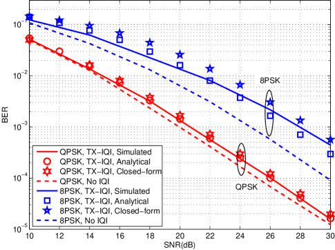
Figure 3: Comparison of analytical and simulated BER performance of the DSTBC-OFDM system under TX-IQI (slow fading, ${{\kappa}_{t}}(dB)=0.5\mathrm{dB}$ and ${{\phi}_{t}}={{3}^{\circ}}$).

Fig. 3 shows the analytical and closed-form BER of QPSK and 8PSK in the presence of TX-IQI in Eq. (31) and Eq. (32), and compares them with the simulated BER. The TX-IQI in simulation is set as the moderate case with ${{\kappa}_{t}}(dB)=0.5\mathrm{dB}$, ${{\phi}_{t}}={{3}^{\circ}}$. The analytical BER of QPSK matches the simulated BER while a small gap is observed in the 8PSK case. The gap is due to both the inaccuracy in modeling severe TX-IQI for the high SINR case, and the Taylor expansion approximation in Eq. (27) because the TX-IQI we assume in the simulation is severe for a first-order Taylor approximation. In addition, according to Eq. (28), the SNR loss caused by TX-IQI should be $0.70$ dB for QPSK and $2.68$ dB for 8PSK, which also matches the simulation results and confirms that 8PSK is less robust to TX-IQI than QPSK, as expected.

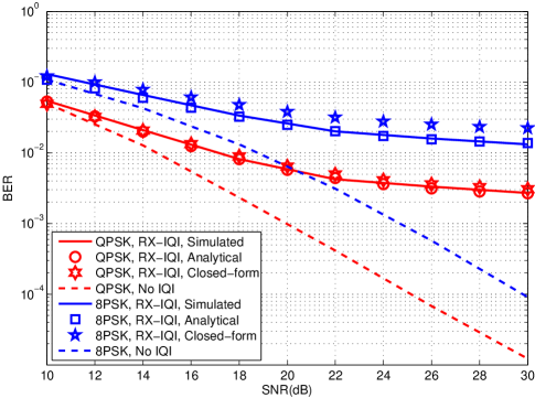
Figure 4: Comparison of analytical and simulated BER performance of the DSTBC-OFDM system under RX-IQI (slow fading, ${{\kappa}_{t}}(dB)=0.5\mathrm{dB}$, ${{\phi}_{t}}={{3}^{\circ}}$).

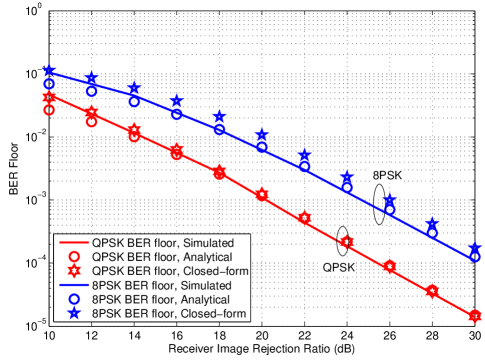
Figure 5: Comparison of analytical and simulated BER floor of the DSTBC-OFDM system under RX-IQI (slow fading, ${{\kappa}_{r}}(dB)=0.5\mathrm{dB}$ and ${{\phi}_{r}}={{3}^{\circ}}$).

Fig. 4 compares the analytical BER in Eq. (40) with the SINR distribution in Eq. (42) and the closed-form BER in Eq. (45). Both of them match the simulated BER results for the RX-IQI case. The RX-IQI parameters are set as the moderate case. It is clear that the BER is much more sensitive to RX-IQI than TX-IQI as shown in Fig. 3. The BER curves of both QPSK and 8PSK show a BER floor in the high SNR region, which is caused by the limited SINR even in the absence of noise. Fig. 5 shows the BER floor of QPSK and 8PSK under RX-IQI for different IRR scenarios. The analytical BER is obtained from Eq. (40) and the closed-form BER floor is obtained from Eq. (45). As shown in Subsection III-B, the BER floors of QPSK and 8PSK for different IRR levels show a $5.5$dB gap in the high IRR region.

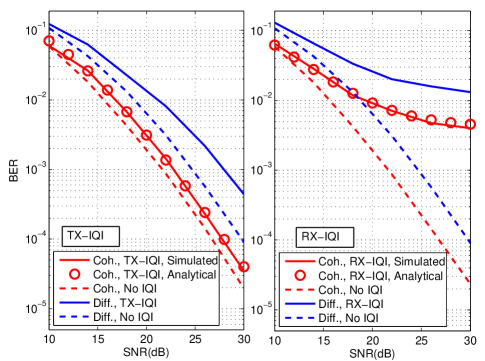
Figure 6: Comparison of BER performance of the differential system and coherent system under IQI (slow fading, ${{\kappa}_{t,r}}(dB)=0.5\mathrm{dB}$ and ${{\phi}_{t,r}}={{3}^{\circ}}$).

Fig. 6 compares the impact of IQI on differential and coherent detection. The channel information in coherent detection is assumed to be perfectly known. As expected, when there is no IQI, the SNR gap between coherent and differential detection is roughly 3dB, and becomes larger in the presence of IQI, especially under RX-IQI. According to Subsection III-D, the performance of coherent detection has an advantage of 3dB in both IRR and SNR. Hence the BER of coherent detection under RX-IQI can be well predicted by setting the noise power $\sigma^{2}$ and the IQI interference power $\rho_{t/r}^{(c)}$ to half of their values in the differential system, which is also shown in the figure. Fig. 7 shows the analytical and closed-form BER of QPSK and 8PSK in the presence of both the TX-IQI and RX-IQI and compares them with the simulated BER. The analytical and closed-form BER are calculated by replacing the noise power term in Eq. (31) and (32) as $\sigma^{2}\rightarrow(\sigma^{2}+\rho_{r})$.

Figure 7: Comparison of analytical and simulated BER floor of the DSTBC-OFDM system under TX-/RX-IQI (slow fading, ${{\kappa}_{t,r}}(dB)=0.5\mathrm{dB}$ and ${{\phi}_{t,r}}={{3}^{\circ}}$)

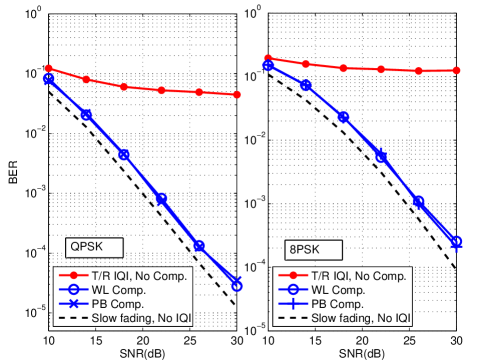
Figure 8: BER performance of the DSTBC-OFDM system under joint TX-/RX-IQI in slow fading channels (${{\kappa}_{t,r}}(dB)=1\mathrm{dB}$, ${{\phi}_{t,r}}={{5}^{\circ}}$).

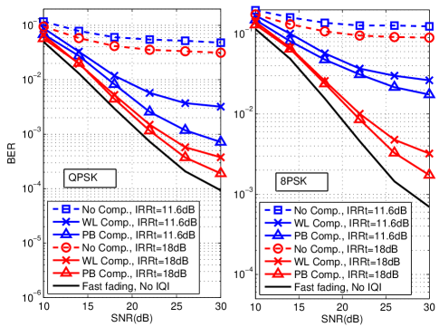
Figure 9: BER performance of the DSTBC-OFDM system under joint TX-/RX-IQI in fast fading channels (when $IRR_{t}=11.6\text{dB}$,${{\kappa}_{t,r}}(dB)=1\mathrm{dB}$, ${{\phi}_{t,r}}={{5}^{\circ}}$); when $IRR_{t}=18\text{dB}$, ${{\kappa}_{t,r}}(dB)=1\mathrm{dB}$, ${{\phi}_{t,r}}={{5}^{\circ}}$).

Fig. 8 shows the performance of our proposed blind IQI compensation algorithms in a slow-fading channel. Both the TX-IQI and RX-IQI parameters are set to severe IQI with ${{\kappa}_{t/r}}(dB)=1\mathrm{dB}$, ${{\phi}_{t/r}}={{5}^{\circ}}$. Both compensation with the PB estimation and WL estimation can effectively mitigate the performance degradation due to IQI. However, we still observe a 1.6dB loss in SNR compared to the IQI-free case for both QPSK and 8PSK modulation. According to our analysis in Subsection IV-A2, even with the perfect compensation matrix, there will be an inevitable SNR loss of $10\mathrm{log}\frac{(1+2|\beta_{t}^{2}|/|\alpha_{t}^{2}|)}{(|\alpha_{t}|-|\beta_{t}|^{2}/|\alpha_{t}|)^{2}}=$1.2dB due to the signal power loss and noise amplification in the compensation of TX-IQI. The rest of SNR loss is caused by the estimation error due to noise. Moreover, Fig. 9 presents the performance of our proposed blind IQI compensation algorithm in a fast-fading channel under joint TX-IQI and RX-IQI. The RX-IQI parameters are set to ${{\kappa}_{r}}(dB)=1\mathrm{dB},{{\phi}_{r}}={{5}^{\circ}}$, while both the moderate TX-IQI case ($\mathrm{IRR}{}_{t}=18$dB) and severe TX-IQI case ($\mathrm{IRR}{}_{t}=11.6$dB) are simulated. A performance degradation is observed in the fast-fading channel even without IQI since the fast-varying channel does not satisfy the quasi-static property required by differential STBC. Moreover, it is clear that the PB estimation outperforms the WL estimation for the fast fading channel. Significant improvement can be observed in the presence of severe TX-IQI. On the other hand, regarding the improvement in BER level after compensation, it is more noticeable for QPSK than that for 8PSK when compared with the WL estimation. However, the SINR improvement due to compensation should be basically the same because the compensation matrices are estimated based on modulated symbols. This is also confirmed by the fact that the SNR gap between the PB estimation and the WL estimation is the same for QPSK and 8PSK modulation.

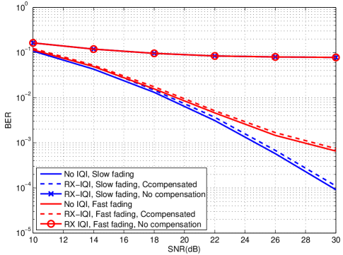
Figure 10: BER performance of the DSTBC-OFDM system under RX-IQI in slow and fast fading channels ($\kappa_{r}(dB)=1\mathrm{dB}$, $\phi_{r}={{5}^{\circ}}$)

The performance of the WL RX-IQI compensation in Subsection IV-A1 is presented in Fig. 10 for both fast-fading and slow-fading channels assuming 8PSK modulation. The RX-IQI parameters are set to ${{\kappa}_{r}}(dB)=1\mathrm{dB}$ and ${{\phi}_{r}}={{5}^{\circ}}$. Fig. 10 shows that the proposed compensation algorithm efficiently compensates for RX-IQI. Since the RX-IQI compensation matrix does not change with the channel, the compensation is effective in both channel scenarios and the degradation caused by RX-IQI is almost eliminated.

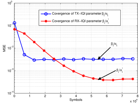
Figure 11: Convergence rate of TX-/RX-IQI parameter estimation (mobile speed 200km, SNR=3dB)

Next, we examined the convergence speed and mean squared error (MSE) of the IQI parameter estimation discussed in Subsection IV-B under severe TX-IQI and RX-IQI in a fast fading channel. The results are shown in Fig. 11. It can be observed from Fig. 11 that the RX-IQI can be estimated more accurately than the TX-IQI parameters. This is due to the fact that the estimation of the TX-IQI parameter is biased by the approximation that the term $\mathbf{B}_{r}^{*}\mathbf{B}_{t}\mathbf{\Lambda}(n)$ in Eq. (84) is ignored.

VI Conclusions

In this paper, we analyzed the impact of TX-IQI and RX-IQI in DSTBC-OFDM. We quantified analytically the BER increase caused by TX-IQI, the BER floor due to RX-IQI and the analytical BER curve of M-PSK under TX-IQI and RX-IQI. The accuracy of these analyses was demonstrated by simulations. In addition, an adaptive decision-directed joint TX-/RX-IQI compensation algorithm for DSTBC-OFDM was proposed and demonstrated to effectively mitigate the performance degradation caused by IQI. We also proposed an enhancement for the high-mobility case by exploiting constrained relationship among a pair of image OFDM subcarriers.

Appendix A BER floor condition under TX-IQI

Since ${{\mathbf{S}}_{k}}{{\mathbf{S}}_{k}}^{H}={{\mathbf{\bar{S}}}_{k}}{{\bar{\mathbf{S}}}_{k}}^{H}=\mathbf{I}$ and ${\mathbf{S}}_{k}$ and ${\mathbf{\bar{S}}}_{k}$ have Alamouti structure, the entries in ${\mathbf{S}}_{k}$ and ${\mathbf{\bar{S}}}_{k}$ satisfy the power constraint of $\left|[{\mathbf{S}}_{k}]_{m,n}\right|^{2}\leq 1,\forall m,n\in[1,2].$ Therefore, according to Eq. (19), the entries of the interference matrix $\Theta_{TX}=|{{\alpha}_{t}}{{\beta}_{t}}|{{\mathbf{S}}_{k}}^{H}\mathbf{{\mathbf{\bar{S}}}}_{k+1}+|{{\alpha}_{t}}{{\beta}_{t}}|{{\mathbf{\bar{S}}}_{k}}^{H}\mathbf{{\mathbf{S}}}_{k+1}$ should satisfy the power constraint: $\left|[\Theta_{TX}]_{m,n}\right|^{2}\leq 2|{{\alpha}_{t}}{{\beta}_{t}}|,\forall m,n\in[1,2]$, which means that the largest error vector magnitude (EVM) introduced by TX-IQI is limited to $2|{{\alpha}_{t}}{{\beta}_{t}}|$. On the other hand, given an M-PSK constellation, the minimum EVM needed to cause a bit error, defined as $A_{min}$, is determined by the distance from a given symbol to the detection boundary of its neighbor in the signal constellation. For 8-PSK signal with normalized power, $A_{min}=\sin\frac{\pi}{8}$. Thus, when the largest EVM introduced by TX-IQI is smaller than $A_{min}$, there will be no error as $\mathrm{SNR}\rightarrow\infty$. In DSTBC-OFDM, the transmitted symbol is normalized by a factor of $\sqrt{2}$, thus the minimum EVM needed to cause a bit error in DSTBC-OFDM is $\frac{A_{min}}{\sqrt{2}}$. Consequently, TX-IQI will not introduce error as $SNR\rightarrow\infty$ unless the maximum error power is larger than $\frac{A_{min}}{\sqrt{2}}$, $i.e.$ $|{{\alpha}_{t}}{{\beta}_{t}}|<\frac{\sqrt{2}}{4}A_{min}$.

Appendix B Derivation of equivalent amplitude loss under TX-IQI

Assume, without loss of generality, that the symbol $u=1/\sqrt{2}$ is transmitted. The symbol error probability could be approximated by the pairwise error probability

$$P_{e,u}\approx P_{e}(u\rightarrow\frac{2\pi}{M})+P_{e}(u\rightarrow-\frac{2\pi}{M})$$ (97)

where $P_{e}(u\rightarrow\frac{2\pi}{M}$) and $P_{e}(u\rightarrow-\frac{2\pi}{M})$ are the probabilities that the transmitted symbol $u$ is detected as $\frac{\pi}{M}$ and $-\frac{\pi}{M}$ at the receiver, respectively. As shown in Fig. 2, an error will occur when the received symbol falls outside the detection boundaries $\overline{OA}$ and $\overline{OB}$ due to the noise effect. In the high SNR case, the probability of error $P_{e}(u\rightarrow\frac{2\pi}{M}$) can be approximated by the probability that the received symbol falls to the other side of line $\overline{OA}$. Likewise, the symbol error probability $P_{e}(u\rightarrow-\frac{2\pi}{M}$) can also be approximated by the probability that the received symbol falls to the other side of line $\overline{OB}$. Under these approximations, the pairwise error probability $P_{e}(u\rightarrow\frac{2\pi}{M}$) and $P_{e}(u\rightarrow-\frac{2\pi}{M})$ is totally determined by the distance from the symbol $u$ to the detection boundaries $\overline{OA}$ and $\overline{OB}$, which are denoted as $D(u,\overline{OA})$ and $D(u,\overline{OB})$, respectively. Hence, when TX-IQI introduces an error vector $\varepsilon$ and a gain $|\alpha_{t}|^{2}$ to the transmitted signal, $i.e$. $u^{\prime}=|\alpha_{t}|^{2}u+\varepsilon$, the distances between the transmitted symbol and the decision boundaries are changed, denoted as $D(u^{\prime},\overline{OA})$ and $D(u^{\prime},\overline{OB})$, so the pairwise error probability becomes $P_{e,u^{\prime}}\approx P_{e}(u^{\prime}\rightarrow\frac{2\pi}{M})+P_{e}(u^{\prime}\rightarrow-\frac{2\pi}{M})$. Define a pair of equivalent signal amplitude losses $\epsilon^{+}\in\mathbf{R}$ and $\epsilon^{-}\in\mathbf{R}$ that satisfy $P_{e}(u^{\prime}\rightarrow\frac{2\pi}{M})=P_{e}\left((u-\epsilon^{+})\rightarrow\frac{2\pi}{M}\right)$ and $P_{e}(u^{\prime}\rightarrow-\frac{2\pi}{M})=P_{e}\left((u-\epsilon^{-})\rightarrow-\frac{2\pi}{M}\right)$, respectively. According to our previous analysis, the distances from $(u-\epsilon^{+})$ and $(u-\epsilon^{-})$ to the corresponding detection boundary should be equal to that of $u^{\prime}$, $i.e.$ $D(u-\epsilon^{+},\overline{OA})=D(u^{\prime},\overline{OA})$ and $D(u-\epsilon^{-},\overline{OB})=D(u^{\prime},\overline{OB})$. Thus, after some geometrical calculations, $\epsilon^{+}$ and $\epsilon^{-}$ are given by

$$\epsilon^{+} = |a_{\varepsilon}|\sin(\varphi_{\varepsilon})\cot(\pi/M)-|a_{\varepsilon}|\cos(\varphi_{\varepsilon})$$

$$\epsilon^{-} = |a_{\varepsilon}|\sin(\varphi_{\varepsilon})\cot(\pi/M)+|a_{\varepsilon}|\cos(\varphi_{\varepsilon})$$ (98)

where $\varphi_{\varepsilon}$ and $|a_{\varepsilon}|$ are the angle and amplitude of the TX-IQI error vector $\varepsilon$. According to our analysis in Section III, $\varepsilon$ is a zero-mean complex Gaussian random variable with variance $|\alpha_{t}\beta_{t}|^{2}$, and $|a_{\varepsilon}|\cos(\varphi_{\varepsilon})$ and $|a_{\varepsilon}|\sin(\varphi_{\varepsilon})$ are the real and imaginary parts of $\varepsilon$, respectively. Hence, they are both zero-mean Gaussian variables with variance $|\alpha_{t}\beta_{t}|^{2}/2$. Consequently, both $\epsilon^{+}$and $\epsilon^{-}$ are real zero-mean Gaussian variable with variance $\left(1+\cot(\pi/M){}^{2}\right)|\alpha_{t}\beta_{t}|^{2}$. Thus, the signal power due to TX-IQI can be expressed as follows

$$E_{s,TX} = (|\alpha_{t}|^{2}/\sqrt{2}-\epsilon)^{2}$$ (99)

$$= (|\alpha_{t}|^{2}/\sqrt{2}+\sqrt{\left(1+\cot(\pi/M){}^{2}\right)|\alpha_{t}\beta_{t}|^{2}/2}n^{\prime})^{2}$$

$$= (|\alpha_{t}|^{2}+\sqrt{\left(1+\cot(\pi/M){}^{2}\right)|\alpha_{t}\beta_{t}|^{2}}n^{\prime})^{2}/2$$

where $\epsilon=\sqrt{\left(1+\cot(\pi/M){}^{2}\right)|\alpha_{t}\beta_{t}|^{2}/2}n^{\prime}$ is the random amplitude loss and $n$ is a real zero-mean Gaussian random variable with variance 1.

Lei Chen received the B.Eng. degree in communication engineering from UESTC, China, in 2010. He is currently a Ph.D. candidate in the National Key Laboratory of Science and Technology on Communications at UESTC. He joined Dr. Naofal Al-Dhahir’s group in University of Texas at Dallas as a visiting Ph.D. student in 2015-2016. His research interests are focused on millimeter-wave communications, especially on the baseband compensation of radio frequency impairments.

Ahemd G. Helmy received the B.Sc. and M.Sc. degrees with honors in electronics and communications engineering from Cairo University, Egypt, in 2008 and 2011, respectively. Currently, he is pursuing his Ph.D degree in Electrical Engineering in wireless communication in the University of Texas at Dallas. His research interests include Digital Signal Processing, Interference Mitigation Techniques for Multi-user MIMO systems, and their applications to various wireless standards, like WLAN and LTE. Calling the industrial background, he had many experiences from working for Apple Inc., Intel Corp., Xtendwave Semiconductors, Wasiela Semiconductors, and different R&D research projects collaborated with many industrial leading labs for IMEC, Vodafone, and Qtel. During that time, he focused on how to homogeneously merge his theoretical background and practical experience together in a tangible output emphasized through ling several patents.

Guangrong Yue received the Ph.D. degrees in communication and information system from UESTC, Chengdu, China, in 2006. He was a Post-Doctoral Fellow at the Department of EECS at University of California, Berkeley from 2007 to 2008. He is now a professor of the National Key Laboratory of Science and Technology on Communications, UESTC. As one of the key researchers, he has participated in the Project of Millimeter Wave and Tera-hertz Key Technology and High-speed Baseband Signal Processing supported by the National High-tech R&D Program of China (863 Program). His major research interests include mobile communications and millimeter-wave communications.

Shaoqian Li (F’16) received the B.S.E. degree in communication technology from Northwest Institute of Telecommunication (Xidian University), China, in 1982, and the M.S.E. degree in communication system from UESTC, China, in 1984. He is a Professor, Ph.D. Supervisor, and the Director of the National Key Laboratory of Science and Technology on Communications, UESTC, and a member of the National High Technology R&D Program (863 Program) Communications Group. His research interests include wireless communication theory and anti-interference technology.

Naofal Al-Dhahir (S’89-M’90-SM’98-F’08) received the Ph.D. degree in electrical engineering from Stanford University. He is the Erik Jonsson Distinguished Professor with The University of Texas at Dallas. From 1994 to 2003, he was a Principal Member of the Technical Staff with GE Research and AT&T Shannon Laboratory. He is co-inventor of 41 issued U.S. patents, co-author of over 325 papers with over 8000 citations, and co-recipient of four IEEE best paper awards. He is the Editor-in-Chief of the IEEE TRANSACTIONS ON COMMUNICATIONS.

References

- [1] S. N. Diggavi, N. Al-Dhahir, A. Stamoulis, and A. R. Calderbank, “Great expectations: The value of spatial diversity in wireless networks,” Proc. IEEE, vol. 92, no. 2, pp. 219–270, Feb. 2004.
- [2] V. Tarokh and H. Jafarkhani, “A differential detection scheme for transmit diversity,” IEEE J. Sel. Areas Commun., vol. 18, no. 7, pp. 1169–1174, Jul. 2000.
- [3] S. N. Diggavi, N. Al-Dhahir, A. Stamoulis, and A. R. Calderbank, “Differential space-time coding for frequency-selective channels,” IEEE Commun. Lett., vol. 6, no. 6, pp. 253–255, Jun. 2002.
- [4] S. Lu and N. Al-Dhahir, “Coherent and differential ICI cancellation for mobile OFDM with application to DVB-H,” IEEE Trans. Wireless Commun., vol. 7, no. 11, pp. 4110 – 4116, Dec. 2008.
- [5] “Radio broadcasting systems: Digital audio broadcasting (DAB) to mobile, portable and fixed receivers,” ETSI EN 300 401, 2001.
- [6] B. L. Hughes, “Differential space-time modulation,” IEEE Trans. Inf. Theory, vol. 46, no. 7, pp. 2567–2578, Nov. 2000.
- [7] A. Tarighat, R. Bagheri, and A. H. Sayed, “Compensation schemes and performance analysis of IQ imbalances in OFDM receivers,” IEEE Trans. Signal Process., vol. 53, no. 8, pp. 3257–3268, Aug. 2005.
- [8] A. Tarighat and A. H. Sayed, “Joint compensation of transmitter and receiver impairments in OFDM systems,” IEEE Trans. Wireless Commun., vol. 6, no. 1, pp. 240–247, Jan. 2007.
- [9] X. Cheng, Z. Luo, and S. Li, “Joint estimation for I/Q imbalance and multipath channel in millimeter-wave SC-FDE systems,” IEEE Trans. Veh. Technol., vol. 65, no. 9, pp. 6901–6912, Sep. 2016.
- [10] M. Petit and A. Springer, “Analysis of a properness-based blind adaptive I/Q filter mismatch compensation,” IEEE Trans. Wireless Commun., vol. 15, no. 1, pp. 781–793, Jan 2016.
- [11] B. Narasimhan, S. Narayanan, H. Minn, and N. Al-Dhahir, “Reduced-complexity baseband compensation of joint Tx/Rx I/Q imbalance in mobile MIMO-OFDM,” IEEE Trans. Wireless Commun., vol. 9, no. 5, pp. 1720–1728, May 2010.
- [12] M. Marey, M. Samir, and M. H. Ahmed, “Joint estimation of transmitter and receiver IQ imbalance with ML detection for Alamouti OFDM systems,” IEEE Trans. Veh. Technol., vol. 62, no. 6, pp. 2847–2853, Jul. 2013.
- [13] D. Tandur and M. Moonen, “STBC MIMO OFDM systems with implementation impairments,” in IEEE Vehicular Technology Conference (VTC-Fall ’08), Sept. 2008, pp. 1–5.
- [14] Y. Zou, M. Valkama, and M. Renfors, “Performance analysis of space-time coded MIMO-OFDM systems under I/Q imbalance,” in IEEE International Conference on Acoustics, Speech and Signal Processing (ICASSP ’07), vol. 3, Apr. 2007, pp. 341–344.
- [15] A. Hakkarainen, J. Werner, K. R. Dandekar, and M. Valkama, “Precoded massive MU-MIMO uplink transmission under transceiver I/Q imbalance,” in 2014 IEEE Globecom Workshops (GC Wkshps), Dec 2014, pp. 320–326.
- [16] U. Oruthota and O. Tirkkonen, “Link adaptation of precoded MIMO-OFDMA system with I/Q interference,” IEEE Trans. Commun., vol. 63, no. 3, pp. 780–790, Mar. 2015.
- [17] N. Kolomvakis, M. Matthaiou, and M. Coldrey, “IQ imbalance in multiuser systems: Channel estimation and compensation,” IEEE Trans. Commun., vol. 64, no. 7, pp. 3039–3051, July 2016.
- [18] J. Gao, X. Zhu, H. Lin, and A. K. Nandi, “Independent component analysis based semi-blind I/Q imbalance compensation for MIMO OFDM systems,” IEEE Trans. Wireless Commun., vol. 9, no. 3, pp. 914–920, March 2010.
- [19] Y. Zou, M. Valkama, and M. Renfors, “Digital compensation of I/Q imbalance effects in space-time coded transmit diversity systems,” IEEE Trans. Signal Process., vol. 56, no. 6, pp. 2496–2508, June 2008.
- [20] J. J. de Witt and G. J. van Rooyen, “A blind I/Q imbalance compensation technique for direct-conversion digital radio transceivers,” IEEE Trans. Veh. Technol., vol. 58, no. 4, pp. 2077–2082, May 2009.
- [21] P. Rykaczewski and F. Jondral, “Blind I/Q imbalance compensation in multipath environments,” in 2007 IEEE International Symposium on Circuits and Systems, May 2007, pp. 29–32.
- [22] L. Chen, A. G. Helmy, G. Yue, S. Li, and N. Al-Dhahir, “Performance and compensation of I/Q imbalance in differential STBC-OFDM,” in 2016 IEEE Global Communications Conference (Globecom2016), Washington, USA, Dec. 2016.
- [23] S. M. Alamouti, “A simple transmit diversity technique for wireless communications,” IEEE J. Sel. Areas Commun., vol. 16, no. 8, pp. 1451–1458, Oct. 1998.
- [24] C.-S. Hwang, S. H. Nam, J. Chung, and V. Tarokh, “Differential space time block codes using nonconstant modulus constellations,” IEEE Trans. Signal Process., vol. 51, no. 11, pp. 2955–2964, 2003.
- [25] C. Xu, L. Wang, S. X. Ng, and L. Hanzo, “Soft-decision multiple-symbol differential sphere detection and decision-feedback differential detection for differential QAM dispensing with channel estimation in the face of rapidly fading channels,” IEEE Trans. Wireless Commun., vol. 15, no. 6, pp. 4408–4425, 2016.
- [26] T. C. Schenk, E. R. Fledderus, and P. F. Smulders, “Performance analysis of zero-IF MIMO OFDM transceivers with IQ imbalance,” Journal of Communications, vol. 2, no. 7, pp. 9–19, 2007.
- [27] M. Torabi, S. Aïssa, and M. R. Soleymani, “On the BER performance of space-frequency block coded OFDM systems in fading MIMO channels,” IEEE Trans. Wireless Commun., vol. 6, no. 4, pp. 1366–1373, Apr. 2007.
- [28] J. Qi and S. Aissa, “Analysis and compensation of I/Q imbalance in MIMO transmit-receive diversity systems,” IEEE Trans. Commun., vol. 58, no. 5, pp. 1546–1556, May 2010.
- [29] M. J. S. Morris H. DeGroot, Probability and Statistics (4th Edition). Addison-Wesley, 2010, pp. 597–599.
- [30] C. Geng, H. Sun, and S. A. Jafar, “On the optimality of treating interference as noise: General message sets,” IEEE Trans. Inf. Theory, vol. 61, no. 7, pp. 3722–3736, Jul. 2015.
- [31] E. Eleftheriou and D. Falconer, “Tracking properties and steady-state performance of RLS adaptive filter algorithms,” IEEE Trans. Acoust. Speech Signal Process., vol. 34, no. 5, pp. 1097–1110, Oct 1986.