The effective neutrino mass of neutrinoless double-beta decays:
how possible to fall into a well

Abstract

The neutrinoless double-beta ($0\nu 2\beta$) decay is currently the only feasible process in particle and nuclear physics to probe whether massive neutrinos are the Majorana fermions. If they are of the Majorana nature and have a normal mass ordering, the effective neutrino mass term $\langle m\rangle_{ee}$ of a $0\nu 2\beta$ decay may suffer significant cancellations among its three components and thus sink into a decline, resulting in a “well” in the three-dimensional graph of $|\langle m\rangle_{ee}|$ against the smallest neutrino mass $m_{1}$ and the relevant Majorana phase $\rho$. We present a new and complete analytical understanding of the fine issues inside such a well, and identify a novel threshold of $|\langle m\rangle_{ee}|$ in terms of the neutrino masses and flavor mixing angles: $|\langle m\rangle_{ee}|_{*}=m_{3}\sin^{2}\theta_{13}$ in connection with $\tan\theta_{12}=\sqrt{m_{1}/m_{2}}$ and $\rho=\pi$. This threshold point, which links the local minimum and maximum of $|\langle m\rangle_{ee}|$, can be used to signify observability or sensitivity of the future $0\nu 2\beta$-decay experiments. Given current neutrino oscillation data, the possibility of $|\langle m\rangle_{ee}|<|\langle m\rangle_{ee}|_{*}$ is found to be very small.

PACS number(s): 14.60.Pq, 13.15.+g, 25.30.Pt

Since Ettore Majorana first formulated a fermionic particle that should be its own antiparticle in 1937 [1], a huge amount of attention has been paid to the Majorana fermions in particle and nuclear physics and the Majorana zero modes in solid-state physics [2]. In particular after the experimental discoveries of solar, atmospheric, reactor and accelerator neutrino oscillations [3], whether massive neutrinos are the Majorana fermions becomes an especially burning question among a number of fundamentally important questions in neutrino physics and cosmology. If this is the case, then the neutrinoless double-beta ($0\nu 2\beta$) decays of some even-even nuclei are expected to take place [4]. Namely, $N(A,Z)\to N(A,Z+2)+2e^{-}$, where the lepton number is violated by two units. Given the fact that the neutrino masses are so small that all the lepton-number-violating processes must be desperately suppressed, currently the unique and only feasible way to demonstrate the Majorana nature of massive neutrinos is to observe the $0\nu 2\beta$ decays. In this respect a number of ambitious experiments are either underway or in preparation [5].

In the standard scheme of three neutrino flavors the rate of a $0\nu 2\beta$ decay is proportional to the squared modulus of the effective Majorana neutrino mass term [6]

$$\langle m\rangle_{ee}=m_{1}|U_{e1}|^{2}e^{{\rm i}\rho}+m_{2}|U_{e2}|^{2}+m_{3}|U_{e3}|^{2}e^{{\rm i}\sigma}\;,$$ (1)

where $m_{i}$ denotes the $i$-th neutrino mass (for $i=1,2,3$), $U_{ei}$ is the corresponding element of the $3\times 3$ neutrino mixing matrix $U$ [8], and $\rho$ and $\sigma$ stand for the Majorana phases. One often chooses to parametrize $|U_{ei}|$ as follows [3]: $|U_{e1}|=\cos\theta_{12}\cos\theta_{13}$, $|U_{e2}|=\sin\theta_{12}\cos\theta_{13}$, and $|U_{e3}|=\sin\theta_{13}$. The three mixing angles $\theta_{12}$, $\theta_{13}$ and $\theta_{23}$ have been determined to a good degree of accuracy from current neutrino oscillation data, so have been the value of $\Delta m^{2}_{21}\equiv m^{2}_{2}-m^{2}_{1}$ and the modulus of $\Delta m^{2}_{31}\equiv m^{2}_{3}-m^{2}_{1}$ [3]. But the sign of $\Delta m^{2}_{31}$ and the two phase parameters in Eq. (1) remain unknown, nor does the absolute neutrino mass scale. That is why $|\langle m\rangle_{ee}|$ is usually plotted as a function of $m_{1}$ in the normal mass ordering (NMO) case ($\Delta m^{2}_{31}>0$) or $m_{3}$ in the inverted mass ordering (IMO) case ($\Delta m^{2}_{31}<0$) by allowing $\rho$ and $\sigma$ to vary from $0$ to $2\pi$ [9]. In such a so-called Vissani graph, a two-dimensional “well” can appear in the NMO situation due to a significant cancellation among the three components of $\langle m\rangle_{ee}$. The bottom of the well signifies the case of $|\langle m\rangle_{ee}|\to 0$ [10], a disappointing possibility which is definitely consistent with the present experimental data.

Two immediate questions are in order: (1) how possible for the three neutrinos to have a NMO; (2) how possible for the actual value of $|\langle m\rangle_{ee}|$ to fall into the well and become unobservable in any realistic $0\nu 2\beta$ experiments. A combination of current atmospheric (Super-Kamiokande [11]) and accelerator-based (T2K [12] and NO$\nu$A [13]) neutrino oscillation data preliminarily favors the NMO at the $2\sigma$ level. If this turns out to be the case, an answer to the second question will be highly desirable because it can help interpret the discovery or null result of a $0\nu 2\beta$ experiment in the standard three-flavor scheme, although some kind of hypothetical (ad hoc) new physics may also contribute to $|\langle m\rangle_{ee}|$.

The present work aims to answer the second question by giving a new and complete analytical understanding of the fine structure of the three-dimensional well of $|\langle m\rangle_{ee}|$ against $m_{1}$ and $\rho$, as illustrated in Fig. 1, where the best-fit values $\Delta m^{2}_{21}=7.54\times 10^{-5}~{}{\rm eV}^{2}$, $\Delta m^{2}_{31}=2.47\times 10^{-3}~{}{\rm eV}^{2}$, $\sin^{2}\theta_{12}=0.308$ and $\sin^{2}\theta_{13}=0.0234$ [14] have been taken as the typical inputs. We identify a novel threshold of $|\langle m\rangle_{ee}|$ which is located at the center of the well: $|\langle m\rangle_{ee}|_{*}=m_{3}\sin^{2}\theta_{13}$ in connection with $\tan\theta_{12}=\sqrt{m_{1}/m_{2}}$ and $\rho=\pi$. This threshold point links the local minimum and maximum of $|\langle m\rangle_{ee}|$, and it can be used to signify the observability or sensitivity of the future $0\nu 2\beta$-decay experiments. Given current neutrino oscillation data, the possibility of $|\langle m\rangle_{ee}|<|\langle m\rangle_{ee}|_{*}$ is found to be very small.

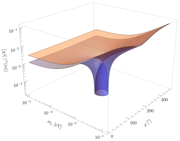
Figure 1: Three-dimensional illustration of the upper (orange) and lower (blue) bounds of $|\langle m\rangle_{ee}|$ as functions of $m_{1}$ and $\rho$ in the NMO case, where the best-fit values $\Delta m^{2}_{21}=7.54\times 10^{-5}~{}{\rm eV}^{2}$, $\Delta m^{2}_{31}=2.47\times 10^{-3}~{}{\rm eV}^{2}$, $\sin^{2}\theta_{12}=0.308$ and $\sin^{2}\theta_{13}=0.0234$ [14] have typically been input.

Fig. 1 shows that the depth of the well of $|\langle m\rangle_{ee}|$ is mainly sensitive to a narrow parameter space of $m_{1}$ and $\rho$, while the other Majorana phase $\sigma$ plays an important role in shaping the bottom of the well [15]. The latter point can be seen in an analytical way as follows. Taking $\displaystyle\frac{\partial|\langle m\rangle_{ee}|}{\partial\sigma}=0$, we obtain

$$\tan\sigma=\frac{m_{1}\sin\rho}{m_{1}\cos\rho+m_{2}\tan^{2}\theta_{12}}\;,$$ (2)

so as to maximize or minimize $|\langle m\rangle_{ee}|$ for the given values of $m_{1}$ and $\rho$. Substituting Eq. (2) into the expression of $|\langle m\rangle_{ee}|$ in Eq. (1), one arrives at the following upper (“U”) and lower (“L”) bounds:

$$\left|\langle m\rangle_{ee}\right|_{\rm U,L}=\left|\overline{m}_{12}\cos^{2}\theta_{13}\pm m_{3}\sin^{2}\theta_{13}\right|\;,$$ (3)

where the sign “$+$” (or “$-$”) corresponds to “U” (or “L”), and

$$\overline{m}_{12}\equiv\sqrt{m^{2}_{1}\cos^{4}\theta_{12}+\frac{1}{2}m_{1}m_{2}\sin^{2}2\theta_{12}\cos\rho+m^{2}_{2}\sin^{4}\theta_{12}}\;\;.$$ (4)

It is easy to understand this result in an intuitive way: for any given values of $m_{1}$ and $\rho$, the maximum of $|\langle m\rangle_{ee}|$ comes out when the sum of the first two components of $\langle m\rangle_{ee}$ has the same phase as the third one (i.e., $\sigma$); and the minimum of $|\langle m\rangle_{ee}|$ arises when the difference between these two phases is equal to $\pm\pi$. The bottom of the well shown in Fig. 1 corresponds to $|\langle m\rangle_{ee}|_{\rm L}=0$, or equivalently

$$\overline{m}_{12}=m_{3}\tan^{2}\theta_{13}\;.$$ (5)

Given the expressions $m_{2}=\sqrt{\displaystyle m^{2}_{1}+\Delta m^{2}_{21}}$ and $m_{3}=\sqrt{\displaystyle m^{2}_{1}+\Delta m^{2}_{31}}$ in the NMO case, Eq. (5) allows us to fix how the two free parameters $m_{1}$ and $\rho$ are correlated with each other. Using the same best-fit inputs of $\Delta m^{2}_{21}$, $\Delta m^{2}_{31}$, $\sin^{2}\theta_{12}$ and $\sin^{2}\theta_{13}$ as those used in plotting Fig. 1, we illustrate the numerical correlation between $m_{1}$ and $\rho$ dictated by Eq. (5) in Fig. 2 — the red curve. Such a correlation curve roughly looks like an ellipse, but a careful analytical check shows that it does not really obey the standard equation of an ellipse. Fig. 2 tells us that touching the bottom of the well (i.e., $|\langle m\rangle_{ee}|\to 0$) is not a highly probable event at all, because it requires $m_{1}$ and $\rho$ to lie in the narrow regions $2~{}{\rm meV}\lesssim m_{1}\lesssim 7~{}{\rm meV}$ and $0.86\lesssim\rho/\pi\lesssim 1.14$, respectively [16].

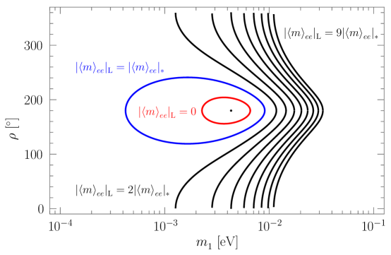
Figure 2: The numerical correlation between $m_{1}$ and $\rho$ in three typical cases: (a) $|\langle m\rangle_{ee}|_{\rm L}=0$ (the red curve); (b) $|\langle m\rangle_{ee}|_{\rm L}=|\langle m\rangle_{ee}|_{*}=m_{3}\sin^{2}\theta_{13}$ (the black dot and the blue curve); and (c) $|\langle m\rangle_{ee}|_{\rm L}=n|\langle m\rangle_{ee}|_{*}$ with $n\geq 2$ (the black curves). Here the best-fit values of $\Delta m^{2}_{21}$, $\Delta m^{2}_{31}$, $\sin^{2}\theta_{12}$ and $\sin^{2}\theta_{13}$ used in plotting Fig. 1 have been input.

Another salient feature of the well is the “bullet”-like structure of $|\langle m\rangle_{ee}|_{\rm L}$ as shown in Fig. 1, corresponding to the parameter space of $\overline{m}_{12}\leq m_{3}\tan^{2}\theta_{13}$. In other words, the surface of this bullet is described by

$$|\langle m\rangle_{ee}|_{\rm L}=m_{3}\sin^{2}\theta_{13}-\overline{m}_{12}\cos^{2}\theta_{13}\;.$$ (6)

The extremum of $|\langle m\rangle_{ee}|_{\rm L}$ in this inner region of the well is supposed to be located at a point fixed by the following two conditions:

$$\frac{\partial\left|\langle m\rangle_{ee}\right|_{\rm L}}{\partial\rho} = \frac{m_{1}m_{2}\sin^{2}2\theta_{12}\cos^{2}\theta_{13}}{4\overline{m}_{12}}\sin\rho=0\;,$$

$$\frac{\partial\left|\langle m\rangle_{ee}\right|_{\rm L}}{\partial m_{1}} = \frac{m_{1}}{m_{3}}\sin^{2}\theta_{13}-\frac{m_{2}\overline{m}^{2}_{12}-\Delta m^{2}_{21}\sin^{2}\theta_{12}\left(m_{2}\sin^{2}\theta_{12}+m_{1}\cos^{2}\theta_{12}\cos{\rho}\right)}{m_{1}m_{2}\overline{m}_{12}}\cos^{2}\theta_{13}=0\;.\hskip 14.22636pt$$ (7)

The first condition definitely leads us to $\rho=0$ or $\pi$. But Fig. 2 clearly shows that $\rho$ should only take a value around $\pi$ inside the well, and thus it is appropriate to take $\rho=\pi$ instead of $\rho=0$. In this case $\overline{m}_{12}=|m_{1}\cos^{2}\theta_{12}-m_{2}\sin^{2}\theta_{12}|$ holds, and the second condition in Eq. (7) is simplified to

$$\frac{\partial\left|\langle m\rangle_{ee}\right|_{\rm L}}{\partial m_{1}}=\frac{m_{1}}{m_{3}}\sin^{2}\theta_{13}\pm\left(\cos^{2}\theta_{12}-\frac{m_{1}}{m_{2}}\sin^{2}\theta_{12}\right)\cos^{2}\theta_{13}=0\;,$$ (8)

where “$\pm$” correspond to the prerequisites $m_{1}<m_{2}\tan^{2}\theta_{12}$ and $m_{1}>m_{2}\tan^{2}\theta_{12}$, respectively. But in reality Eq. (8) can never be fulfilled since its second term is much larger than its first term as a result of (a) $2.50\times 10^{-1}\leq\sin^{2}\theta_{12}\leq 3.54\times 10^{-1}$ and $1.85\times 10^{-2}\leq\sin^{2}\theta_{13}\leq 2.46\times 10^{-2}$ at the $3\sigma$ level [14] and (b) $m_{1}/m_{3}\leq m_{1}/m_{2}$ in the NMO case. Nevertheless, Eq. (8) can at least allow us to draw a conclusion that is absolutely consistent with current experimental data:

$$\frac{\partial\left|\langle m\rangle_{ee}\right|_{\rm L}}{\partial m_{1}} > 0\hskip 11.38092pt{\rm for}\hskip 11.38092ptm_{1}<m_{2}\tan^{2}\theta_{12}\;,\hskip 14.22636pt$$

$$\frac{\partial\left|\langle m\rangle_{ee}\right|_{\rm L}}{\partial m_{1}} < 0\hskip 11.38092pt{\rm for}\hskip 11.38092ptm_{1}>m_{2}\tan^{2}\theta_{12}\;.$$ (9)

This observation means that $|\langle m\rangle_{ee}|_{\rm L}$ increases when $m_{1}<m_{2}\tan^{2}\theta_{12}$ holds, and it decreases when $m_{1}>m_{2}\tan^{2}\theta_{12}$ holds. Hence there must be a local maximum for $|\langle m\rangle_{ee}|_{\rm L}$, denoted as

$$|\langle m\rangle_{ee}|_{*}=m_{3}\sin^{2}\theta_{13}=\sqrt{m^{2}_{1}+\Delta m^{2}_{31}}\ \sin^{2}\theta_{13}$$ (10)

at the position fixed by $\rho=\pi$ and

$$m_{1}=m_{2}\tan^{2}\theta_{12}=\sqrt{m^{2}_{1}+\Delta m^{2}_{21}}\tan^{2}\theta_{12}\;\;\;\;{\Longrightarrow}\;\;\;\;m_{1}=\sqrt{\Delta m^{2}_{21}}\ \frac{\sin^{2}\theta_{12}}{\sqrt{\displaystyle\cos 2\theta_{12}}}\;.$$ (11)

In Fig. 1 this point is exactly the tip of the bullet inside the well! In other words, the local maximum of $|\langle m\rangle_{ee}|_{\rm L}$ arises from Eq. (6) at $\overline{m}_{12}=0$. Given the best-fit values of $\Delta m^{2}_{21}$, $\Delta m^{2}_{31}$, $\sin^{2}\theta_{12}$ and $\sin^{2}\theta_{13}$ that have been used in plotting Fig. 1, the numerical location of the tip of the bullet turns out to be $\left(m_{1},\rho,|\langle m\rangle_{ee}|_{*}\right)\simeq\left(4~{}{\rm meV},180^{\circ},1~{}{\rm meV}\right)$.

The above analysis explains why the bottom of the well does not converge to a single point and why it is not flat either. In a similar way one can understand why there is a local minimum for $|\langle m\rangle_{ee}|_{\rm U}$, as shown in Fig. 1. The extremum of $|\langle m\rangle_{ee}|_{\rm U}$ is expected to be located at a position determined by

$$\frac{\partial\left|\langle m\rangle_{ee}\right|_{\rm U}}{\partial\rho} = \frac{m_{1}m_{2}\sin^{2}2\theta_{12}\cos^{2}\theta_{13}}{4\overline{m}_{12}}\sin\rho=0\;,$$

$$\frac{\partial\left|\langle m\rangle_{ee}\right|_{\rm U}}{\partial m_{1}} = \frac{m_{1}}{m_{3}}\sin^{2}\theta_{13}+\frac{m_{2}\overline{m}^{2}_{12}-\Delta m^{2}_{21}\sin^{2}\theta_{12}\left(m_{2}\sin^{2}\theta_{12}+m_{1}\cos^{2}\theta_{12}\cos{\rho}\right)}{m_{1}m_{2}\overline{m}_{12}}\cos^{2}\theta_{13}=0\;.\hskip 22.76228pt$$ (12)

Of course, only $\rho=\pi$ is allowed with respect to the first condition in Eq. (12). The second condition in Eq. (12) can never be satisfied for the same realistic reasons given below Eq. (8). An analogous and straightforward analysis tells us that the local minimum of $|\langle m\rangle_{ee}|_{\rm U}$ exactly coincides with the local maximum of $|\langle m\rangle_{ee}|_{\rm L}$, and thus both of them are described by Eqs. (10) and (11). This interesting result explains why the upper (in orange) and lower (in blue) bounds of $|\langle m\rangle_{ee}|$ connect with each other in Fig. 1 when $m_{1}=\sqrt{m^{2}_{1}+\Delta m^{2}_{21}}\tan^{2}\theta_{12}$ and $\rho=\pi$ hold. Note that the overlap of the local maximum of $|\langle m\rangle_{ee}|_{\rm L}$ and the local minimum of $|\langle m\rangle_{ee}|_{\rm U}$ can also be understood from Eq. (3) itself. At $m_{1}=\sqrt{m^{2}_{1}+\Delta m^{2}_{21}}\tan^{2}\theta_{12}$ and $\rho=\pi$, one simply has $|\langle m\rangle_{ee}|_{\rm L}=|\langle m\rangle_{ee}|_{\rm U}=m_{3}\sin^{2}\theta_{13}$ as a consequence of $\overline{m}_{12}=0$. So $|\langle m\rangle_{ee}|_{*}=m_{3}\sin^{2}\theta_{13}\simeq 1~{}{\rm meV}$ stands for a threshold of $|\langle m\rangle_{ee}|$ in the NMO case.

To visualize the steepness of the slope of $|\langle m\rangle_{ee}|_{\rm L}$ around the well in Fig. 1, let us project its contour onto the $m_{1}$-$\rho$ plane by taking $|\langle m\rangle_{ee}|_{\rm L}=n|\langle m\rangle_{ee}|_{*}$ (for $n=0,1,2,\cdots$) in Fig. 2. It is especially interesting to compare between the contours of the well at its bottom with $|\langle m\rangle_{ee}|_{\rm L}=0$ (the red curve) and at its threshold height with $|\langle m\rangle_{ee}|_{\rm L}=|\langle m\rangle_{ee}|_{*}$ (the blue curve and the black point). They clearly show how the well becomes narrower when the value of $|\langle m\rangle_{ee}|_{\rm L}$ goes down. The profile of $|\langle m\rangle_{ee}|_{\rm L}$ will be partially open and thus lose its “well” feature as $|\langle m\rangle_{ee}|_{\rm L}\geq 2|\langle m\rangle_{ee}|_{*}$ is taken into account. Now that $|\langle m\rangle_{ee}|_{\rm L}>|\langle m\rangle_{ee}|_{*}$ always holds outside the blue curve in Fig. 2, we argue that the parameter space of $|\langle m\rangle_{ee}|_{\rm L}\leq|\langle m\rangle_{ee}|_{*}$ (i.e., $0.4~{}{\rm meV}\lesssim m_{1}\lesssim 10~{}{\rm meV}$ and $0.66\lesssim\rho/\pi\lesssim 1.34$) is a simple measure of the chance for $|\langle m\rangle_{ee}|$ to fall into the well and become completely unobservable.

In general, $|\langle m\rangle_{ee}|$ depends on all the three unknown parameters $m_{1}$, $\rho$ and $\sigma$. To illustrate how probable or improbable for $|\langle m\rangle_{ee}|$ to have a value smaller than $|\langle m\rangle_{ee}|_{*}$ in a more explicit way, we plot the three-dimensional parameter space of $m_{1}$, $\rho$ and $\sigma$ in Fig. 3, where the best-fit values of $\Delta m^{2}_{21}$, $\Delta m^{2}_{31}$, $\sin^{2}\theta_{12}$ and $\sin^{2}\theta_{13}$ used in plotting Figs. 1 and 2 have been input. For clarity, the intersecting surfaces on the $\rho$-$\sigma$ plane corresponding to $m_{1}=1,2,4$ and 6 meV are specified in the figure. One can see that this parameter space is very small as compared with the whole cubic space (i.e., the whole regions of $m_{1}$, $\rho$ and $\sigma$ allowed by current experimental constraints). In comparison with $m_{1}$ and $\rho$, the phase $\sigma$ is only weakly constrained in Fig. 3. When the first two components of $\langle m\rangle_{ee}$ in Eq. (1) essentially cancel each other out (i.e., $2~{}{\rm meV}\lesssim m_{1}\lesssim 7~{}{\rm meV}$ and $0.86\lesssim\rho/\pi\lesssim 1.14$), a large part of the range of $\sigma$ is allowed (e.g., the black intersecting surface corresponding to $m_{1}=4$ meV in Fig. 3). But when the value of $m_{1}$ decreases, the value of $\sigma$ should approach $\pi$, such as the green intersecting surface corresponding to $m_{1}=1$ meV in Fig. 3. In this case the second component of $\langle m\rangle_{ee}$ in Eq. (1) can be cancelled by the other two components to a maximal level. For a similar reason, the value of $\sigma$ should approach 0 or $2\pi$ when the value of $m_{1}$ increases (e.g., the blue intersecting surface corresponding to $m_{1}=6$ meV in Fig. 3). In any case we conclude that the possibility of $|\langle m\rangle_{ee}|<|\langle m\rangle_{ee}|_{*}$ involves significant cancellations among its three components and is really small.

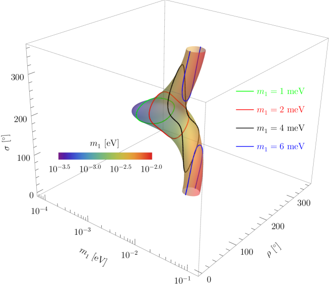
Figure 3: The parameter space of $m_{1}$, $\rho$ and $\sigma$ allowed for $|\langle m\rangle_{ee}|<|\langle m\rangle_{ee}|_{*}$ to hold, where the best-fit values of $\Delta m^{2}_{21}$, $\Delta m^{2}_{31}$, $\sin^{2}\theta_{12}$ and $\sin^{2}\theta_{13}$ used in plotting Fig. 1 have been input. The intersecting surfaces for $m_{1}=1,2,4$ and 6 meV on the $\rho$-$\sigma$ plane are explicitly shown in the figure.

From an experimental point of view, the threshold $|\langle m\rangle_{ee}|_{*}$ should signify an ultimate limit of the reachable sensitivity to $|\langle m\rangle_{ee}|$ in the foreseeable future. At present the most sensitive $0\nu 2\beta$-decay experiments can only set an upper limit of $|\langle m\rangle_{ee}|$ around $165~{}{\rm meV}$ [17], which depends on some theoretical uncertainties in calculating the relevant nuclear matrix elements [18]. The most ambitious next-generation high-sensitivity $0\nu 2\beta$-decay experiments (e.g., nEXO [19]) are likely to probe $|\langle m\rangle_{ee}|$ at the level of a few tens of meV [5], a sensitivity still much larger than the threshold value $|\langle m\rangle_{ee}|_{*}\simeq 1~{}{\rm meV}$ . In this sense there would be no hope to observe any $0\nu 2\beta$-decay signal if $|\langle m\rangle_{ee}|$ were unfortunately around or below the value of $|\langle m\rangle_{ee}|_{*}$ in the standard three-flavor scheme.

Before ending our discussions about $\langle m\rangle_{ee}$ and its possible parameter space in the NMO case, let us briefly comment on the relationship $\tan\theta_{12}=\sqrt{m_{1}/m_{2}}$ from a model-building point of view. This condition, together with $\rho=\pi$, allows for $|\langle m\rangle_{ee}|=|\langle m\rangle_{ee}|_{*}=m_{3}\sin^{2}\theta_{13}$ as a remarkable threshold. It is well known that the Cabibbo angle $\theta_{\rm C}$ of quark flavor mixing can be related to the ratio of quark masses $m_{d}$ and $m_{s}$ in a class of models [22]: $\tan\theta_{\rm C}\simeq\sqrt{m_{d}/m_{s}}~{}$, which is consistent with the experimental data to a good degree of accuracy. In comparison, the possibility of $\tan\theta_{12}\simeq\sqrt{m_{1}/m_{2}}$ is also interesting, in particular when the NMO is true for the three mass eigenstates of $\nu_{e}$, $\nu_{\mu}$ and $\nu_{\tau}$ neutrinos. For example, we find that an effective Majorana neutrino mass matrix of the form

$$M_{\nu}=\left(\begin{matrix}0&A&A\cr A&B&C\cr A&C&B\cr\end{matrix}\right)-m_{3}\frac{\sin\theta_{13}}{\sqrt{2}}\left(\begin{matrix}\sqrt{2}\ \sin\theta_{13}&+{\rm i}&-{\rm i}\cr+{\rm i}&0&0\cr-{\rm i}&0&0\cr\end{matrix}\right)\;,$$ (13)

where $A$, $B$ and $C$ are all real, can essentially predict $|\langle m\rangle_{ee}|=m_{3}\sin^{2}\theta_{13}$ and $\tan\theta_{12}=\sqrt{m_{1}/m_{2}}$ together with $\theta_{23}=\pi/4$, $\delta=-\pi/2$, $\rho=\pi$ and $\sigma=0$ in the standard parametrization of $U$. Because $M_{\nu}$ possesses the exact $\mu$-$\tau$ reflection symmetry, which can easily be simplified to the $\mu$-$\tau$ permutation symmetry in the $\theta_{13}\to 0$ limit, one may take it as a starting point to build a phenomenological neutrino mass model in this connection [23].

In summary, we have achieved some new and important insights into the effective neutrino mass $\langle m\rangle_{ee}$ of the $0\nu 2\beta$ decays in the NMO case — a case which seems to be more likely than the IMO case according to today’s preliminary experimental data. Because $|\langle m\rangle_{ee}|$ depends not only on the unknown neutrino mass $m_{1}$ but also on the free Majorana phases $\rho$ and $\sigma$, a novel three-dimensional presentation of $|\langle m\rangle_{ee}|$ against $m_{1}$ and $\rho$ reveals an intriguing “well” structure in the NMO case. The present work provides a new and complete analytical understanding of the fine issues inside such a well. We find a particularly interesting threshold of $|\langle m\rangle_{ee}|$ in terms of the neutrino masses and flavor mixing angles: $|\langle m\rangle_{ee}|_{*}=m_{3}\sin^{2}\theta_{13}$ in connection with $\tan\theta_{12}=\sqrt{m_{1}/m_{2}}$ and $\rho=\pi$. We suggest that this threshold point, which links the local minimum and maximum of $|\langle m\rangle_{ee}|$, be used to signify observability or sensitivity of the future $0\nu 2\beta$-decay experiments. In view of current neutrino oscillation data, we conclude that the possibility of $|\langle m\rangle_{ee}|<|\langle m\rangle_{ee}|_{*}$ must be very small. In other words, it should be very promising to detect a signal of the $0\nu 2\beta$ decays and verify the Majorana nature of massive neutrinos in a foreseeable future, even if they have a normal mass spectrum.

One of us (Z.Z.X.) would like to thank J. Angel and S.T. Petcov for interesting communications during the DBD16 workshop in Osaka, where this work was initiated. We are also grateful to Y.F. Li, J. Zhang and S. Zhou for some useful discussions, and to Z.C. Liu and Y. Lu for their kind helps in plotting the figures. This work is supported in part by the National Natural Science Foundation of China under grant No. 11135009 (Z.Z.X.) and grant No. 11605081 (Z.H.Z.).

References

[1] E. Majorana, Nuovo Cimento 14, 171 (1937).
[2] S.R. Elliott and M. Franz, Rev. Mod. Phys. 87, 137 (2015).
[3] C. Patrignani et al. (Particle Data Group),
Chin. Phys. C 40, 100001 (2016).
[4] W.H. Furry, Phys. Rev. 15, 1184 (1939).
[5] For a recent review with extensive references, see:
S.M. Bilenky and C. Giunti, Int. J. Mod. Phys. A 30, 0001
(2015); S. Dell’Oro, S. Marcocci, M. Viel and F. Vissani,
Adv. High Energy Phys. 2016, 2162659 (2016);
J.D. Vergados, H. Ejiri and F. Simkovic, arXiv:1612.02924.
[6] S.M. Bilenky, J. Hosek and S.T. Petcov,
Phys. Lett. B 94, 495 (1980); J. Schechter and J.W.F. Valle,
Phys. Rev. D 22, 2227 (1980); M. Doi, T. Kotani, H. Nishiura,
K. Okuda and E. Takasugi, Phys. Lett. B 102, 323 (1981).
[7] Z.Z. Xing and Y.L. Zhou, Chin. Phys. C 39,
011001 (2015); Mod. Phys. Lett. A 30, 1530019 (2015);
Adv. Ser. Direct. High Energy Phys. 25, 157 (2015).
[8] Z. Maki, M. Nakagawa and S. Sakata,
Prog. Theor. Phys. 28, 870 (1962);
B. Pontecorvo, Sov. Phys. JETP 26, 984 (1968).
[9] F. Vissani, JHEP 06, 022 (1999).
[10] W. Rodejohann, Nucl. Phys. B 597, 110 (2001);
Z.Z. Xing, Phys. Rev. D 68, 053002 (2003);
W. Rodejohann, Int. J. Mod. Phys. E 20, 1833 (2011);
S. Dell’oro, S. Marcocci and F. Vissani, Phys. Rev. D 90,
033005 (2014).
[11] See, e.g., B. Rebel, talk given at the XIV International
Conference on Topics in Astroparticle and Underground Physics,
September 2015, Torino, Italy.
[12] K. Abe et al., Phys. Rev. Lett. 112,
181801 (2014).
[13] See, e.g., C. Kachulis, talk given at the EPS
Conference on High Energy Physics, July 2015, Vienna, Austria.
[14] F. Capozzi et al., Phys. Rev. D 89,
093018 (2014). See also F. Capozzi et al.,
Nucl. Phys. B 908, 218 (2016);
D.V. Forero, M. Tortola and J.W.F. Valle,
Phys. Rev. D 90, 093006 (2014); M.C. Gonzalez-Garcia,
M. Maltoni and T. Schwetz, JHEP 1411, 052 (2014).
[15] Z.Z. Xing, Z.H. Zhao and Y.L. Zhou, Eur. Phys. J.
C 75, 423 (2015).
[16] See also G. Benato, Eur. Phys. J. C 75, 563 (2015).
[17] A. Gando et al. (KamLAND-Zen Collaboration),
Phys. Rev. Lett. 117, 082503 (2016).
[18] J. Engel and J. Menendez, arXiv:1610.06548.
[19] Y. Lin, talk given a the APR15 meeting of APS, 2015.
[20] S.F. Ge and M. Lindner, arXiv:1608.01618.
[21] S. Pascoli and S.T. Petcov, Phys. Rev. D 77, 113003 (2008).
[22] S. Weinberg, in Transactions of the New York
Academy of Sciences38, 185 (1977); F. Wilczek and A. Zee,
Phys. Lett. B 70, 418 (1977); H. Fritzsch, Phys. Lett. B 70, 436 (1977); B 73, 317 (1978);
F. Vissani, Phys. Lett. B 508, 79 (2001). For a review, see:
H. Fritzsch and Z.Z. Xing, Prog. Part. Nucl. Phys. 45, 1 (2000).
[23] For the latest review with extensive references,
see: Z.Z. Xing and Z.H. Zhao, Rept. Prog. Phys. 79, 076201 (2016).