Impact of a locally measured $H_{0}$ on the interpretation of cosmic chronometer data

Abstract

Whereas many measurements in cosmology depend on the use of integrated distances or time, galaxies evolving passively on a time scale much longer than their age difference allow us to determine the expansion rate $H(z)$ solely as a function of the redshift-time derivative $dz/dt$. These model-independent ‘cosmic chronometers’ can therefore be powerful discriminators for testing different cosmologies. In previous applications, the available sources strongly disfavoured models (such as $\Lambda$CDM) predicting a variable acceleration, preferring instead a steady expansion rate over the redshift range $0\lesssim z\lesssim 2$. A more recent catalog of 30 objects appears to suggest non-steady expansion. In this paper, we show that such a result is entirely due to the inclusion of a high, locally-inferred value of the Hubble constant $H_{0}$ as an additional datum in a set of otherwise pure cosmic-chronometer measurements. This $H_{0}$, however, is not the same as the background Hubble constant if the local expansion rate is influenced by a Hubble Bubble. Used on their own, the cosmic chronometers completely reverse this conclusion, favouring instead a constant expansion rate out to $z\sim 2$.

1 Introduction

Cosmological measurements usually rely on the use of integrated (luminosity or angular) distances, which unavoidably introduces a model dependence in the data themselves. For example, the use of Type Ia supernovae as ‘standard candles’ to measure the distance scale relies on finding the ‘correct’ lightcurve shape needed to determine their absolute luminosity. The parameters defining this estimator are optimized along with the parameters of the assumed cosmological model, necessitating a recalibration of the data for each and every model being tested (Perlmutter et al. 1998; Riess et al. 1998; Schmidt et al. 1998; Melia 2012; Wei et al. 2013). Galaxies evolving passively on a time scale much larger than their age difference can instead be used to measure the expansion rate $H(z)$ using solely the local redshift-time derivative $dz/dt$ (Jimenez & Loeb 2002). As we shall explain in greater detail below, these are typically massive (with a stellar content $>10^{11}\;M_{\odot}$) early-type galaxies that formed over $\sim 90\%$ of their stellar mass at high-redshifts ($z>2-3$, i.e., before the Universe was $\sim 4$ Gyr old) very rapidly (in only $\sim 0.1-0.3$ Gyr) and have experienced only minor subsequent episodes of star formation. They are believed to be the oldest objects at all redshifts (Treu et al. 2005), and if we observe them at $z\sim 1$ (i.e., when the Universe was $\sim 7$ Gyr old), we see a stellar population that mostly formed during the first $\sim 2-10\%$ of the galaxies’ evolution. These so-called cosmic chronometers therefore avoid the need of pre-assuming a cosmological model in order to extract the data, and can therefore form a powerful discriminant to test different expansion scenarios.

In previous applications, we (Melia  Maier 2013; Melia & McClintock 2015) used the then available catalog of sources to compare two specific models: the $R_{\rm h}=ct$ universe (Melia 2007, 2016a, 2017; Melia & Shevchuk 2012) and the standard (concordance) $\Lambda$CDM model. In these one-on-one comparative tests, the use of information criteria showed that the cosmic chronometers strongly preferred $R_{\rm h}=ct$ over $\Lambda$CDM. The significance of this result is that, whereas the standard model requires a transition from deceleration at large redshifts to an accelerated expansion today, the $R_{\rm h}=ct$ universe predicts a constant expansion rate at all redshifts.

Recently, however, 5 new, valuable data points were added to the compilation of $H(z)$ measurements at that critical redshift ($z\sim 0.5$) where the transition is thought to have occurred (Moresco et al. 2016), thereby improving the statistical significance of the fits in the redshift range $0\lesssim z\lesssim 1$. Based on a study of this expanded sample, direct evidence for the existence of an epoch of cosmic re-acceleration was claimed to have been seen. To reach this result, however, the locally measured, high value of $H_{0}$ had to be included in the data set. Yet this determination of the Hubble constant is completely distinct from all the other measurements based on the cosmic chronometers themselves. In this paper, we argue that this step has unduly biased this recent analysis and that—contrary to its conclusion—the expanded sample in fact strengthens the case for a constant expansion rate in the redshift range $0\lesssim z\lesssim 2$.

2 The Hubble Bubble

When one ignores the effects of the local gravitational potential at the position of the observer, the value of $H_{0}$ measured directly from the redshift-distance relation of local sources is discrepant at a level of $\sim 2.4\sigma$ (or roughly $9\%$) relative to the Hubble constant inferred from fitting anisotropies in the cosmic microwave background (CMB) using $\Lambda$CDM (Marra et al. 2013; Planck Collaboration 2014). Generally speaking, our observations of the Universe are made from a vantage point whose spacetime differs from the mean by a degree that is very difficult to probe with any precision (Valkenburg et al. 2014). Estimates of the cosmic variance created by local inhomogeneities are often based on the Hubble Bubble picture, in which a sphere of matter is carved out of the Friedmann-Robertson-Walker (FRW) background, and is compressed or diluted in order to obtain a simple distribution of the ensuing inhomogeneity with a slightly different FRW spacetime.

Detailed analysis of the dependence of the measurement of $H_{0}$ on the local gravitational potential has shown that the Hubble Bubble effect can at least partially mitigate the $\sim 9\%$ tension between the CMB and local Hubble constants (Marra et al. 2013). Compelling observational support for this interpretation of the disparity is provided by the fact that local measurements of $H_{0}$ using supernovae within $74h^{-1}$ Mpc (corresponding roughly to $z=0.023$) is $6.5\%\pm 1.8\%$ larger than the value of $H_{0}$ measured using supernovae outside of this region. Consequently, one can largely alleviate the Hubble Bubble effect by adopting a minimum redshift of $0.023$ in the analysis of the expansion rate.

The idea that we may be living in a local underdense Hubble Bubble has actually been considered since the 1990’s (Turner et al. 1992; Suto et al. 1995; Shi et al. 1996, 1998; Zehavi et al. 1998; Giovanelli et al. 1999). In every case, the implied variation on the local gravitational potential was shown to generate variance of the cosmological parameters, including the local Hubble constant. The general consensus from all this work is that the locally measured value of $H_{0}$, though obtained in a model-independent fashion, is nonetheless high (compared to what one might expect in the context of other cosmological measurements) with systematic uncertainties that are difficult to ascertain with any precision.

For this principal reason, we believe that a test of cosmological models using measurements of $H(z)$ is more robust when only the truly model-independent data obtained with cosmic chronometers are used, without the contamination introduced through the inclusion of a poorly understood measurement of $H_{0}$. Our approach is bolstered by the fact that the results of the model comparisons could not be more different when the locally measured $H_{0}$ is included versus when it is not, even with exactly the same sample of 30 cosmic-chronometer measurements. But if the expansion rate measured with this technique firmly points to an epoch of cosmic re-acceleration (Moresco et al. 2016), then this should be seen regardless of whether or not $H_{0}$ is added to the data set.

3 Model Comparisons

To demonstrate this point compellingly, we will here use the most recent sample of 30 cosmic-chronometer measurements to compare seven different models, including $\Lambda$CDM. In so doing, we shall re-affirm, and strengthen, the conclusions drawn from our previous two studies (Melia & Maier 2013; Melia & McClintock 2015)—that measurements of $H(z)$ using cosmic chronometers strongly favour the constant expansion rate predicted by the $R_{\rm h}=ct$ universe over other models, including $\Lambda$CDM. The models we will compare are as follows:

1. The standard flat $\Lambda$CDM model, in which the matter and dark-energy densities are fixed by the condition $\Omega_{\Lambda}=1-\Omega_{\rm m}$. Throughout this paper, $\Omega_{i}$ is the energy density $\rho_{i}$ of species $i$, scaled to today’s critical density, $\rho_{c}\equiv 3c^{2}H_{0}^{2}/8\pi G$. In this model, the two free parameters are $H_{0}$ and $\Omega_{\rm m}$, and

   $$H^{\Lambda{\rm CDM}}(z)=H_{0}\left[\Omega_{\rm m}(1+z)^{3}+\Omega_{\rm r}(1+z)^{4}+\Omega_{\Lambda}\right]^{1/2}\;.$$ (1)

2. The concordance o$\Lambda$CDM model, with free parameters $H_{0}$, $\Omega_{\rm m}$, and $\Omega_{\Lambda}$. In this model,

   $$H^{o\Lambda{\rm CDM}}(z)=H_{0}\left[\Omega_{\rm m}(1+z)^{3}+\Omega_{\rm r}(1+z)^{4}+\Omega_{\Lambda}+\Omega_{k}(1+z)^{2}\right]^{1/2}\;.$$ (2)

3. The flat $w$CDM model, in which the matter and dark-energy densities are fixed by the condition $\Omega_{\rm de}=1-\Omega_{\rm m}$, but with an unconstrained dark-energy equation-of-state, $w_{\rm de}\equiv p_{\rm de}/\rho_{\rm de}$, where $p_{\rm de}$ is the pressure. The three free parameters here are $H_{0}$, $\Omega_{\rm m}$, and $w_{\rm de}$, with an expansion rate give by

   $$H^{w{\rm CDM}}(z)=H_{0}\left[\Omega_{\rm m}(1+z)^{3}+\Omega_{\rm r}(1+z)^{4}+\Omega_{\rm de}(1+z)^{3(1+w_{\rm de})}\right]^{1/2}\;.$$ (3)

4. Einstein–de Sitter space, in which the cosmic fluid contains only matter. $H_{0}$ is the sole free parameter, and

   $$H^{\rm EdS}(z)=H_{0}(1+z)^{3/2}\;.$$ (4)

5. A Friedmann model (that we shall call Friedmann I) with negative curvature. Here, $\Omega_{\rm m}$ is fixed to be $0.3$ and $\Omega_{\Lambda}=0$, implying a curvature term with $\Omega_{\rm k}=1-\Omega_{\rm m}=0.7$ (Baryshev & Teerikorpi 2012). In this case, $H_{0}$ is the sole free parameter, and

   $$H^{\rm Friedmann\;I}(z)=H_{0}\left[\Omega_{\rm m}(1+z)^{3}+\Omega_{\rm k}(1+z)^{2}\right]^{1/2}\;.$$ (5)

6. A Friedmann model (that we shall call Friedmann II) with negative curvature, but with $\Omega_{\rm m}$ free and $\Omega_{\Lambda}=0$, implying a curvature term with $\Omega_{\rm k}=1-\Omega_{\rm m}$. In this case, the two free parameters are $H_{0}$ and $\Omega_{\rm m}$, and

   $$H^{\rm Friedmann\;II}(z)=H^{\rm Friedmann\;I}(z)\;.$$ (6)

7. The $R_{\rm h}=ct$ universe (a Friedmann-Robertson-Walker cosmology with zero active mass). In this model, the total equation-of-state is $\rho+3p=0$, with $\rho$ and $p$ the total energy density and pressure of the cosmic fluid (Melia 2007, 2016a, 2017; Melia & Shevchuk 2012). In this cosmology, $H_{0}$ is the sole free parameter, and

   $$H^{R_{\rm h}=ct}(z)=H_{0}(1+z)\;.$$ (7)

We test these models collectively against measurements of the Hubble constant using the passively evolving galaxies introduced above, based on the observed 4,000 Å break in their spectra. For old stellar populations, this break is a discontinuity in the spectral continuum due to metal absorption lines whose amplitude correlates linearly with the age and metal abundance of the stars (Moresco et al. 2016). It is weakly dependent on the star formation history, and is basically unaffected by dust reddening. When the metallicity of these stars is known, it is possible to measure the age difference $\Delta t$ of two nearby galaxies as proportional to the difference in their 4,000 Å amplitudes. The slope of this proportionality depends on the metallicity. Then, together with the measured redshift difference $\Delta z$ of these galaxies, one may find the Hubble constant at the average of their redshifts using the simple relation

$$H(z)=-{1\over(1+z)}\,{dz\over dt}\approx-{1\over(1+z)}\,{\Delta z\over\Delta t}\;.$$ (8)

Of course, there are several factors that may inhibit the accuracy of this procedure, possibly mitigating the value of using differential measurements of age in these systems. Fortunately, extensive tests (Moresco et al. 2016) have shown that the 4,000 Å feature depends principally on the age and metallicity of the host galaxies, but only weakly on the assumed star formation history, the initial mass function, a possible progenitor bias, and the so-called $\alpha$-enhancement. The latter refers to the observation that these early, passive galaxies have higher ratios of $\alpha$ elements to iron than Milky-Way type galaxies. And the progenitor bias may arise due to a possible evolution of the mean redshift of formation as a function of redshift of the galaxy samples.

Of these effects, it turns out that only an uncertainty in the metallicity contributes noticeably to a systematic error $\sigma_{\rm sys}$ comparable to the statistical errors in the sample. Simulations have shown that the progenitor bias contributes at most only a few percentage points to $\sigma_{\rm sys}$, while the impact of the initial mass function is insignificant. The difference between the 4,000 Å amplitudes estimated in a single stellar population using a Chabrier or Salpeter initial mass function is less than $0.3\%$ for all reasonable metallicities and less than $0.2\%$ for the solar metallicity (Moresco et al. 2016). The difference in the 4,000 Å amplitudes due to the $\alpha$-enhancement is likewise extremely small, on average only $\sim 0.5\%$.

The only factor other than metallicity that contributes noticeably to $\sigma_{\rm sys}$ is the star formation history. Again, simulations have shown that variations in the assumed star forming rate can lead to $\lesssim 13\%$ errors in the inferred value of $\Delta z$ from measurements of the 4,000 Å amplitudes (Moresco et al. 2016). Together, the combination of uncertainties in the star formation history and the metallicity contribute an overall error of about $20\%$ to $\Delta z$, and hence the inferred value of $H(z)$.

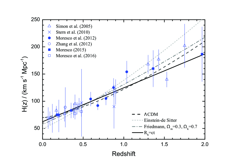
Figure 1: Thirty model-independent measurements of $H(z)$ versus $z$, with error bars, and the best-fit curves from four models (see text). The corresponding likelihood of each model being the best choice is shown in Table 1.

The data are shown in Figure 1 (Moresco et al. 2016; Simon et al. 2005; Stern et al. 2010; Moresco et al. 2012; Zhang et al. 2014; Moresco 2015). For each model, we find the set of parameters that optimize the fit and minimize the $\chi^{2}$. The best-fit curves of four cosmologies are also shown in this figure, superimposed on the data. As we have discussed in earlier papers (Melia & Maier 2013; Melia & McClintock 2015), building on the sound arguments developed in Liddle (2004, 2007) and Liddle et al. (2006), among others, a fair statistical comparison between models with different formulations and numbers of free parameters must be based on the use of information criteria (Takeuchi 2000; Tan & Biswas 2012). In this context, the likelihood of model $\alpha$ being the best choice is given by the expression

$$L_{\alpha}={\exp(-{\rm IC}_{\alpha}/2)\over\sum_{i}\exp(-{\rm IC}_{i}/2)}\;,$$ (9)

where IC_α is one of AIC_α, KIC_α, or BIC_α, and the sum in the denominator runs over all the models being tested simultaneously. The Akaike Information Criterion is defined by ${\rm AIC}=\chi^{2}+2f$, while the Kullback implementation has ${\rm KIC}=\chi^{2}+3f$, and ${\rm BIC}=\chi^{2}+f({\rm ln}\;n)$ is the Bayes information criterion. In these expressions, $f$ is the number of free parameters and $n$ is the number of data points. All of these criteria punish models with a large number of free parameters because these are deemed to be fitting the noise. Also, as discussed in these earlier works, the BIC is the most appropriate criterion to use when $n$ is large, as we have here (with 30 source measurements). But for completeness, we tabulate the results of all three criteria (see Table 1). This tabulation includes the individual IC’s and each model’s likelihood, weighed against all the seven cosmologies being tested simultaneously, of being the best choice. Table 1 also includes the optimized parameters for models that have them, along with their $1\sigma$ uncertainties.

Table 1: Best-fitting Results in Different Cosmological Models

Model	$H_{0}$	$\Omega_{\rm m}$	$\Omega_{\Lambda}$	$w_{\rm de}$	$\chi^{2}_{\rm dof}$	Bayes IC	Kullback IC	Akaike IC
	(km/s/Mpc)					BIC Prob	KIC Prob	AIC Prob
$R_{\rm h}=ct$	$62.3^{+1.5}_{-1.4}$	–	–	–	0.57	20.02 0.50	19.62 0.44	18.62 0.30
$\Lambda$CDM	$68.2^{+2.4}_{-2.8}$	$0.32^{+0.06}_{-0.05}$	$1-\Omega_{\rm m}$	–	0.52	21.30 0.26	20.50 0.28	18.50 0.32
Friedmann II	$61.8^{+3.6}_{-3.5}$	$0.03^{+0.17}_{-0.17}$	–	–	0.59	23.31 0.10	22.51 0.10	20.51 0.12
$w$CDM	$70.8^{+7.2}_{-6.9}$	$0.32^{+0.05}_{-0.06}$	–	$-1.25^{+0.57}_{-0.65}$	0.53	24.56 0.05	23.36 0.07	20.36 0.12
o$\Lambda$CDM	$69.0^{+3.4}_{-6.7}$	$0.36^{+0.19}_{-0.22}$	$0.77^{+0.32}_{-0.48}$	–	0.54	24.66 0.05	23.46 0.06	20.46 0.12
Friedmann I	$57.4^{+1.3}_{-1.3}$	$0.30$ (fixed)	–	–	0.74	24.87 0.04	24.47 0.04	23.47 0.03
Einstein-de Sitter	$49.0^{+1.2}_{-1.1}$	–	–	–	1.74	53.90 2E-8	53.50 2E-8	52.50 1E-8

It is clear from this comparison that when the high, locally measured value of $H_{0}$ is excluded from the data compilation, the cosmic chronometers favour the $R_{\rm h}=ct$ cosmology, which predicts a constant expansion rate over the redshift range $0\lesssim z\lesssim 2$. Flat $\Lambda$CDM is second on the list, but only because we assumed prior values for $w_{\rm de}=-1$ and $k=0$. In principle, all of the free parameters in each model should be optimized using solely the cosmic chronometers for a statistically fair comparison. And we can see that when fewer prior values are assumed, e.g., as for $w$CDM and o$\Lambda$CDM, their probabilities drop considerably.

From the compilation in Table 1, we can also see how sensitive each of the model fits is to the choice of $H_{0}$. Notice, for example, that in the case of $R_{\rm h}=ct$, which has only one free parameter (the Hubble constant itself), the optimized value of $H_{0}$ is very tightly constrained. A $1-\sigma$ variation may be generated with a mere change of only $\pm 1.5$ km s^-1 Mpc^-1. On the other hand, in a model such as $w$CDM, which has three free parameters—and therefore more flexibility—a $1-\sigma$ variation requires a change in $H_{0}$ of about $\pm 7$ km s^-1 Mpc^-1 from its optimum value.

In spite of this clear separation in the model outcomes, however, a possible concern with this analysis is the fact that all of the $\chi^{2}_{\rm dof}$ values listed in Table 1, with the exception of Einstein-de Sitter, are significantly smaller than $1$, suggesting that the errors in Figure 1 may be over-estimated. This may mitigate the tension between certain models and the data, perhaps even producing a biased likelihood of some cosmologies relative to the others. To test whether our conclusions are affected in this way, we have carried out a parallel comparative analysis of these measurements by artificially reducing the errors by a factor (equal to $0.75$, as it turns out) that makes these $\chi^{2}_{\rm dof}$ values approximately equal to $1$ for all but the Einstein-de Sitter universe. The results are shown in Table 2. The likelihoods have indeed changed somewhat, and $w$CDM and $\Lambda$CDM are disfavoured less, though the information criteria still prefer $R_{\rm h}=ct$. On the other hand, the BIC probabilities for $R_{\rm h}=ct$ and standard flat $\Lambda$CDM are now indistinguishable. But on the basis of these results, with artifically reduced errors, one still cannot conclude that the cosmic chronometers favour an accelerating universe. This outcome is qualitatively similar to that based on the analysis of the published measurements and their errors.

Table 2: Best-fitting Results with errors artificially reduced by $25\%$ to make $\chi^{2}_{\rm dof}\sim 1$ in Most Cases

Model	$H_{0}$	$\Omega_{\rm m}$	$\Omega_{\Lambda}$	$w_{\rm de}$	$\chi^{2}_{\rm dof}$	Bayes IC	Kullback IC	Akaike IC
	(km/s/Mpc)					BIC Prob	KIC Prob	AIC Prob
$\Lambda$CDM	$68.2^{+1.9}_{-2.1}$	$0.32^{+0.04}_{-0.03}$	$1-\Omega_{\rm m}$	–	0.92	32.58 0.42	31.78 0.43	29.78 0.42
$R_{\rm h}=ct$	$62.4^{+1.1}_{-1.1}$	–	–	–	1.02	32.95 0.35	32.55 0.29	31.55 0.17
$w$CDM	$70.8^{+6.4}_{-4.8}$	$0.32^{+0.04}_{-0.05}$	–	$-1.25^{+0.37}_{-0.59}$	0.95	35.73 0.09	34.53 0.11	31.53 0.17
o$\Lambda$CDM	$69.0^{+2.9}_{-4.7}$	$0.36^{+0.14}_{-0.17}$	$0.77^{+0.22}_{-0.38}$	–	0.95	35.91 0.08	34.71 0.10	31.71 0.16
Friedmann II	$61.8^{+2.7}_{-2.6}$	$0.03^{+0.13}_{-0.11}$	–	–	1.05	36.16 0.07	35.36 0.07	33.36 0.07
Friedmann I	$57.4^{+1.0}_{-1.0}$	$0.30$ (fixed)	–	–	1.32	41.57 0.005	41.17 0.004	40.17 0.002
Einstein-de Sitter	$49.1^{+0.9}_{-0.8}$	–	–	–	3.10	93.18 3E-14	92.78 2E-14	91.78 1E-14

4 Conclusions

Adding five new measurements of the Hubble parameter $H(z)$ with the cosmic-chronometer approach, Moresco et al. (2016) claimed to obtain the first cosmology-independent constraint on the transition redshift, showing the existence of an epoch of cosmic re-acceleration. This result, however, relies heavily on the use of a Gaussian prior on the Hubble constant, $H_{0}=73\pm 2.4$ km s^-1 Mpc^-1. It is generally recognized that this $H_{0}$ is not an accurate representation of the smoothed background $H_{0}$ if the local expansion rate is influenced by a Hubble Bubble. The inclusion of this high, locally measured value of $H_{0}$ unfairly biases the results by contaminating the cosmic-chronometer data with a measurement whose systematics are unknown.

In this regard, we point out that all of the optimized values of $H_{0}$ in Table 1 are smaller than the locally measured Hubble constant, even for $\Lambda$CDM. In fact, were one to use the cosmic chronometers to infer $H_{0}$ in the context of the standard model, one would actually find a remarkable consistency with the value ($67.8\pm 0.9$ km s^-1 Mpc^-1) measured by Planck (Planck Collaboration 2014). Since the same cosmology is being referenced for the interpretation of these two disparate sets of data, this consistency with the value of $H_{0}$ seen at intermediate and very high redshifts adds some support to our thesis in this paper that the locally measured Hubble constant is not a true representation of its large-scale, smoothed value.

Still, the fact that the optimized value of $H_{0}$ in $R_{\rm h}=ct$ is notably smaller than that in the standard model merits some attention. The Hubble constant cannot be measured directly using Type Ia SNe (since $H_{0}$ is degenerate with the absolute SN magnitude, which is also free). The most accurate determination of $H_{0}$ we have today is from the anisotropies in the CMB (Planck Collaboration 2014). The chronometer-measured value of $H_{0}$ in $R_{\rm h}=ct$ is about $8\%$ smaller than the Planck measurement. But the CMB value of $H_{0}$ is itself model dependent, and the temperature fluctuation spectrum has not yet been analyzed using $R_{\rm h}=ct$. All we have at the moment is the Hubble constant optimized for $\Lambda$CDM, so it is too early to tell whether the chronometer and CMB measurements of $H_{0}$ are consistent with each other in the $R_{\rm h}=ct$ model. What we do know from simulations is that a local Hubble Bubble can probably modify the large-scale value of $H_{0}$ by possibly $\pm 2-3$ km s^-1 Mpc^-1 (Marra et al. 2013; Ben-Dayan et al. 2014), so to be compatible with the low value of $H_{0}$ reported here for $R_{\rm h}=ct$, the future measurement of the Hubble constant in this model based on CMB anisotropies ought to be $\lesssim 65$ km s^-1 Mpc^-1.

It is also worth pointing out that some local measurements of $H_{0}$ do actually suggest a value smaller than that (i.e., $73$ km s^-1 Mpc^-1) employed by Moresco et al. (2016). For example, Tammann & Reindl (2013) used red-giant branch stars in the haloes of local galaxies to calibrate the Type Ia SN luminosity and inferred a Hubble constant $H_{0}=64.0^{+1.6}_{-2.0}$ km s^-1 Mpc^-1, while the (now somewhat dated) SN HST Project yielded a value $H_{0}=62.3^{+1.3}_{-5.0}$ (Sandage et al. 2006). Still, the majority of local measurements of $H_{0}$ suggest a higher value, so the key question for $R_{\rm h}=ct$ remains how the cosmic chronometer measurements will compare with those based on model fits to the CMB temperature anisotropies.

With these caveats in mind, we have demonstrated in this paper that the inference of re-acceleration is reversed when the additional $H_{0}$ datum is excluded. We have shown that, used on their own, without the prior on $H_{0}$, the latest compilation of 30 model-independent cosmic-chronometer measurements prefer a constant expansion rate over an accelerated one out to $z\sim 2$.

This result may seem surprising at first, but it merely confirms the outcome of many previous comparative tests between $\Lambda$CDM and the constant expansion rate cosmology $R_{\rm h}=ct$. This type of analysis has been carried out using diverse sets of data, at low, intermediate, and high redshifts. The $R_{\rm h}=ct$ model appears to be favoured over $\Lambda$CDM by all the observations used so far. A brief survey of the results includes the following sample: (1) When the supernovae in the Supernova Legacy Survey Sample are correctly recalibrated for each model being tested, these favour $R_{\rm h}=ct$ over $\Lambda$CDM with a BIC likelihood of $\sim 90\%$ versus $\sim 10\%$ (Wei et al. 2015); (2) According to the quasar Hubble diagram and the Alcock-Pacźynski test (López-Corredoira et al. 2016; Melia & López-Corredoira 2016), $R_{\rm h}=ct$ is more likely to be correct than $\Lambda$CDM; (3) Based on the presumed constancy of the gas mass fraction in clusters, the BIC favours $R_{\rm h}=ct$ over $\Lambda$CDM with a likelihood of $\sim 95\%$ versus only $\sim 5\%$ (Melia 2016b); (4) While $\Lambda$CDM cannot account for the appearance of high-$z$ quasars without some anomalous seed formation or greatly super-Eddington accretion, none of which have ever been seen, their formation and growth are fully consistent with the timeline predicted in $R_{\rm h}=ct$ (Melia 2013); (5) A similar time-compression problem arises with the emergence of high-$z$ galaxies in $\Lambda$CDM, though not in $R_{\rm h}=ct$ (Melia 2014); (6) Based on the age-redshift relationship of Old Passive Galaxies, the BIC favours $R_{\rm h}=ct$ over $\Lambda$CDM with a likelihood of $\sim 81\%$ versus $\sim 19\%$ (Wei et al. 2015). (7) Whereas the inferred probability of $\Lambda$CDM accounting for the Cosmic Microwave Background (CMB) angular correlation function is $<0.3\%$, $R_{\rm h}=ct$ fits it much better, including the absence of correlation at angles greater than $60^{\circ}$ (Melia 2014). This tension between $\Lambda$CDM and observations of the CMB may be quite serious because the lack of any large-angle correlation is inconsistent with inflationary scenarios. Yet the standard model would not survive without inflation to fix the horizon problem. In contrast, the $R_{\rm h}=ct$ universe does not have or need inflation.

This is only a small sample of the many tests completed thus far, but already it spans a broad range of data, some at low redshifts, others at high redshifts. In every case, the $R_{\rm h}=ct$ cosmology has been favoured over $\Lambda$CDM. Even so, the challenge of establishing the viability of $R_{\rm h}=ct$ is ongoing. In this paper, we have added to the observational evidence in its favour, but several important issues need to resolved. It remains to be seen whether big bang nucleosynthesis (BBN) in this model can correctly reproduce the light elements. Initial attempts at simulating BBN with a constant expansion rate have been very promising, showing that the well-known ⁷Li anomaly plaguing the standard model may be solved by the slower burning taking place with such an expansion scenario (Benoit-Lévy & Chardin 2012). Of course, this won’t be known for sure until the BBN calculations will have been carried out correctly for the conditions in $R_{\rm h}=ct$. Also, although the anisotropies in the CMB have been analyzed for $R_{\rm h}=ct$ in terms of their angular correlation function, they have yet to be used to calculate a power spectrum in this cosmology. As is well known, the ability of $\Lambda$CDM to accurately account for the CMB power spectrum provides strong support in its favour. This analysis, however, is beyond the scope of the present work, and its results will be reported elsewhere.

References

- (1) Baryshev, Y. & Teerikorpi, P. 2012, Fundamental Questions of Practical Cosmology, Springer, Dordrecht
- (2) Ben-Dayan, I., Durrer, R., Marozzi, G. and Schwarz, D. J. 2014, PRL, 112, 221301
- (3) Benoit-Lévy, A. & Chardin, G. 2012, A&A, 537, id.A78
- (4) Giovanelli, R., Dale, D., Haynes, M., Hardy, E. & Campusano, L. 1999, ApJ, 525, 25
- (5) Jimenez, R. & Loeb, A. 2002, ApJ, 573, 37
- (6) Liddle, A. R. 2004, MNRAS, 351, L49
- (7) Liddle, A. R. 2007, MNRAS, 377, L74
- (8) Liddle, A., Mukherjee, P. & Parkinson, D. 2006, Astron. & Geophys., 47, id.040000
- (9) López-Corredoira, M., Melia, F., Lusso, E. & Risaliti, G. 2016, IJMP-D, 25, id.1650060
- (10) Marra, V., Amendola, L., Sawicki, I. & Valkenburg, W. 2013, PRL, 110, id.241305
- (11) Melia, F. 2007, MNRAS, 382, 1917
- (12) Melia, F. 2012, AJ, 144, id.110
- (13) Melia, F. 2013, ApJ, 764, id.72
- (14) Melia, F. 2014, AJ, 147, id.120
- (15) Melia, F. 2014, A&A, 561, id.A80
- (16) Melia, F. 2016a, Front. Phys., 11 (4), id.119801
- (17) Melia, F. 2016b, Proc. R. Soc. A, 472, id.20150765
- (18) Melia, F. 2017, Front. Phys., 12 (1), id.129802
- (19) Melia, F. & López-Corredoira, M. 2016, IJMP-D, submitted (arXiv:1503.05052)
- (20) Melia, F. & Maier, R. S. 2013, MNRAS, 432, 2669
- (21) Melia, F. & McClintock, T. M. 2015, AJ, 150, id.119
- (22) Melia, F. & Shevchuk, A.S.H. 2012, MNRAS, 419, 2579
- (23) Moresco, M. 2015, MNRAS, 450, L16
- (24) Moresco, M., Cimatti, A., Jimenez, R. et al. 2012, JCAP, 8, id.006
- (25) Moresco, M., Pozzetti, L., Cimatti, A., Jimenez, R., Maraston, C., Verde, L., Thomas, D., Citro, A., Tojeiro, R. & Wilkinson, D. 2016, JCAP, 05, id.014
- (26) Perlmutter, S., Aldering, G., della Valle, M. et al. 1998, Nature, 391, 51
- (27) Planck Collaboration. 2014, A&A, 571, id.A23
- (28) Riess, A. G., Filippenko, A. V., Challis, P. et al. 1998, AJ, 116, 1009
- (29) Sandage, A., Tammann, G. A., Saha, A., Reindl, B., Macchetto, F. D., & Panagia, N. 2006, ApJ, 653, 843
- (30) Schmidt, B. P., Suntzeff, N. B., Phillips, M. M. et al. 1998, ApJ, 507, 46
- (31) Shi, X.-D. & Turner, E. L. 1998, AJ, 493, 519
- (32) Shi, X., Widrow, L. M. & Dursi, L. J. 1996, MNRAS, 281, 565
- (33) Simon, J., Verde, L. & Jimenez, R. 2005, PRD, 71, id.123001
- (34) Stern, D., Jimenez, R., Verde, L., Stanford, S. A. & Kamionkowski, M. 2010, ApJS, 188, id.280
- (35) Suto, Y., Suginohara, T. & Inagaki, Y. 1995, Prog. Theor. Phys., 93, 839
- (36) Takeuchi, T. T. 2000, Astrophys. Sp. Sci., 271, 213
- (37) Tammann, G. A. & Reindl, B. 2013, A&A, 549, id A136
- (38) Tan, M.Y.J. & Biswas, R. 2012, MNRAS, 419, 3292
- (39) Treu, T., Ellis, R. S., Liao, T. X., van Dokkum, P. G., Tozzi, P., Coil, A., Newman, J., Cooper, M. C. and Davis, M. 2005, ApJ, 633, 174
- (40) Turner, E. L., Cen, R. & Ostriker, J. P. 1992, AJ, 103, 1427
- (41) Valkenburg, W., Marra, V. & Clarkson, C. 2014, MNRAS, 438, L6
- (42) Wang, Y., Spergel, D. N. & Turner, E. L. 1998, ApJ, 498, 1
- (43) Wei, J.-J., Wu, X. & Melia, F. 2013, ApJ, 772, id.43
- (44) Wei, J.-J., Wu, X., Melia, F. & Maier, F. 2015, AJ, 149, id.10
- (45) Wei, J.-J., Wu, X., Melia, F., Wang, F. Y. & Yu, H. 2015, AJ, 150, id.35
- (46) Zehavi, I., Riess, A. G., Kirshner, R. P. & Dekel, A. A 1998, ApJ, 503, 483
- (47) Zhang, C., Zhang, H., Yuan, S. et al. 2014, Res. Astron. and Astrophys., 14, 1221