Period spacings in red giants

Abstract

Context. The power of asteroseismology relies on the capability of global oscillations to infer the stellar structure. For evolved stars, we benefit from unique information directly carried out by mixed modes that probe their radiative cores. This third article of the series devoted to mixed modes in red giants focuses on their coupling factors that remained largely unexploited up to now.

Aims. With the measurement of the coupling factors, we intend to give physical constraints on the regions surrounding the radiative core and the hydrogen-burning shell of subgiants and red giants.

Methods. A new method for measuring the coupling factor of mixed modes is set up. It is derived from the method recently implemented for measuring period spacings. It runs in an automated way so that it can be applied to a large sample of stars.

Results. Coupling factors of mixed modes were measured for thousands of red giants. They show specific variation with mass and evolutionary stage. Weak coupling is observed for the most evolved stars on the red giant branch only; large coupling factors are measured at the transition between subgiants and red giants, as well as in the red clump.

Conclusions. The measurement of coupling factors in dipole mixed modes provides a new insight into the inner interior structure of evolved stars. While the large frequency separation and the asymptotic period spacings probe the envelope and the core, respectively, the coupling factor is directly sensitive to the intermediate region in between and helps determining its extent. Observationally, the determination of the coupling factor is a prior to precise fits of the mixed-mode pattern, and can now be used to address further properties of the mixed-mode pattern, as the signature of the buoyancy glitches and the core rotation.

1 Introduction

The seismic observations of large sets of stars with the CoRoT and Kepler missions, from the main sequence (Chaplin et al. 2011) up to the red giant branch (De Ridder et al. 2009), has motivated intense work in stellar physics, among which is ensemble asteroseismology (e.g. Kallinger et al. 2010; Mosser et al. 2010; Huber et al. 2011; Silva Aguirre et al. 2011; Kallinger et al. 2014). Ensemble asteroseismology is efficient for evolved stars as they host mixed modes that behave as gravity modes in the core and as pressure modes in the envelope. These modes directly probe the stellar core and, therefore, reveal unique information.

Contrary to pressure modes, evenly spaced in frequency, and to gravity modes, evenly spaced in period, mixed modes show a more complicated frequency pattern. Since, for red giants, the density of gravity modes is large compared to the density of pressure modes, the mixed-mode pattern resembles a pure gravity-mode pattern perturbed by the pressure-mode pattern. The period spacings are close to the asymptotic value for gravity-dominated mixed modes, but are significantly smaller near expected pure pressure modes (e.g., Mosser et al. 2015). Pressure-dominated mixed modes have lower inertia than gravity-dominated mixed modes, hence show larger amplitudes (Dupret et al. 2009; Grosjean et al. 2014). Even with period spacings far from the asymptotic values, they allowed us in a first step to distinguish stars with hydrogen-burning shell from stars with core helium-burning (Bedding et al. 2011; Mosser et al. 2011a). In a second step, the asymptotic analysis of the mixed-mode pattern allowed us to derive precise information on the Brunt-Väisälä frequency profile in the radiative core (Mosser et al. 2012b). Indeed, the asymptotic expansion (Shibahashi 1979; Unno et al. 1989; Mosser et al. 2012b; Takata 2016) is a powerful tool for investigating mixed modes in red giants observed by the space missions CoRoT and Kepler, despite the fact that observations are not conducted in an asymptotic regime. Observed radial pressure orders are small, too small for lying in the asymptotic regime, as shown by CoRoT observations (e.g., De Ridder et al. 2009; Mosser et al. 2010). However, Mosser et al. (2013b) have demonstrated that the second-order asymptotic expansion provides a coherent view on the pressure mode pattern, even for the most evolved red giants (Mosser et al. 2013a). Conversely, high radial gravity orders are observed in mixed modes, except in subgiants, so that considering a first-order expansion for the gravity contribution is relevant (Mosser et al. 2014).

This work allowed us to measure asymptotic period spacings and to derive unique information on stellar evolution. The contraction of the helium core of hydrogen-shell-burning red giants is marked by the decrease of the asymptotic period spacing. Moreover, stars with a degenerate helium core (with a mass inferior to about 1.8 $M_{\odot}$) on the red giant branch (RGB) show a close relationship between the large separation and the period spacing, which is the seismic signature of the mirror effect between the core and the envelope structures. In the red clump, core-helium burning stars with a mass lower than about 1.8 $M_{\odot}$ show a tight mass-dependent relation between the asymptotic large separation and period spacing, contrary to more massive stars.

The use of the mixed modes for assessing the inner interior structure of red giants is, however, still in its infancy. Up to now, only the period spacings have benefitted from large scale measurements (Vrard et al. 2016). Another important parameter, the coupling factor $q$ was precisely determined for a handful of stars only (Buysschaert et al. 2016). This parameter benefitted from a recent breakthrough since Takata (2016) could derive an asymptotic expression for dipole modes using the JWKB method (Jeffreys, Wentzel, Kramers, and Brillouin), taking the perturbation of the gravitational potential into account, but without using the weak-coupling approximation, contrary to the previous work by Unno et al. (1989).

Here, we use the method developed by Mosser et al. (2015) (Paper I of the series) in order to complete the large-scale analysis of Vrard et al. (2016) (Paper II of the series). We specifically address the measurement of the coupling factor $q$ of mixed modes. This parameter plays an important role in the asymptotic expansion: it expresses the link between the pressure and gravity contributions to the mixed mode, respectively expressed by their phases $\theta_{\mathrm{p}}$ and $\theta_{\mathrm{g}}$. Following Unno et al. (1989), the asymptotic expansion reads

$$\tan\theta_{\mathrm{p}}=q\tan\theta_{\mathrm{g}},$$ (1)

with the phases defined as

$$\theta_{\mathrm{g}} = \pi{1\over\Delta\Pi_{1}}\left({\displaystyle{1\over\nu}-\displaystyle{1\over\nu_{\mathrm{g}}}}\right),$$ (2)

$$\theta_{\mathrm{p}} = \pi{\nu-\nu_{\mathrm{p}}\over\Delta\nu_{\mathrm{p}}},$$ (3)

where $\nu_{\mathrm{p}}$ and $\nu_{\mathrm{g}}$ are the asymptotic frequencies of pure pressure and gravity modes, respectively, and $\Delta\nu_{\mathrm{p}}$ is the frequency difference between the consecutive pure pressure radial modes with radial orders ${n_{\mathrm{p}}}$ and ${n_{\mathrm{p}}}+1$, as defined by Mosser et al. (2015).

While $\theta_{\mathrm{p}}$ and $\theta_{\mathrm{g}}$ respectively account for the propagation of the wave in the envelope and in the core, the coupling factor comes from the contribution of the region between the Brunt-Väisälä cavity and the Lamb profile $S_{\ell}=\sqrt{\ell(\ell+1)}\,c/r$ where the oscillation is evanescent. Hence, studying the coupling factor $q$ provides a direct way to examine the evanescent region, namely the physical regions surrounding the hydrogen-burning shell, where most of the stellar luminosity is produced. This parameter plays also a crucial role for examining rotational splittings (Goupil et al. 2013; Deheuvels et al. 2015) and mode visibilities (Mosser et al. 2016), so that its thorough examination becomes crucial in red giant seismology.

The article is organized as follows. Section 2 presents the framework of our analysis. We use the weak-coupling cases in order to illustrate and emphasize how $q$ is linked to stellar interior properties. We also introduce the strong-coupling case, which is necessary at various evolutionary stages. In Section 3, we develop a specific method for measuring the coupling factors in an automated way. Section 4 presents the results derived from the set of Kepler red giants analyzed by Vrard et al. (2016). Results are discussed in Section 5.

2 Coupling factor of mixed modes

In this Section, we show how the coupling factor of mixed modes can be used to probe the stellar interior. We restrain the analysis to dipole mixed modes ($\ell=1$).

2.1 Evanescent region

The coupling factor in Eq. (1) measures the decay of the wave in the region between the cavities delimited by the Brunt-Väisälä frequency $N_{\mathrm{BV}}$ and the Lamb frequency $S_{1}$ (Fig. 1). This intermediate zone is called the evanescent region. In the JWKB approximation, thus assuming that the wavelength of the oscillations is much shorter than the scale height of the equilibrium stellar structure, the radial component of the wavevector $\kappa$ in the evanescent region can be written

$$\kappa={\sqrt{(S_{1}^{2}-\omega^{2})(\omega^{2}-N_{\mathrm{BV}}^{2})}\over c\,\omega},$$ (4)

where $c$ is the sound speed and $\omega$ is the angular frequency.

We assume in the following that the evanescent zone is located between the hydrogen-burning shell and the base of the convective envelope. The Brunt-Väisälä and Lamb frequencies show similar radial variations in this region probed by the mixed modes (Fig. 1 and, e.g., Fig. 2 of Montalbán et al. 2012). Both can be approximated with a power law with similar exponent:

$$-{\mathrm{d}\ln N_{\mathrm{BV}}\over\mathrm{d}\ln r}=\beta_{N}\simeq\beta\simeq\beta_{S}=-{\mathrm{d}\ln S_{1}\over\mathrm{d}\ln r}.$$ (5)

In fact, the exponent $\beta$ measures the density contrast between the core and the envelope: the higher the contrast, the higher $\beta$. We expect $\beta$ to increase with the evolution and contraction of the core. In evolved red giants, where the density contrast between the envelope and the core is high enough to ensure that the local gravity varies as $r^{-2}$ in the evanescent region, $\beta$ is expected to be close to the upper limit of 3/2 (Takata 2016).

As a consequence of the parallel variations of $N_{\mathrm{BV}}$ and $S_{1}$, the ratio

$$\alpha=N_{\mathrm{BV}}/S_{1}$$ (6)

can be considered as nearly uniform in the region above the hydrogen-burning shell where the oscillation is evanescent. A very thin evanescent zone means $\alpha$ close to unity, whereas a wide one has a small $\alpha$. In the following, we use this ratio $\alpha$ as a measure of the extent of the evanescent region and aim at linking $\alpha$ and $\beta$ with $q$.

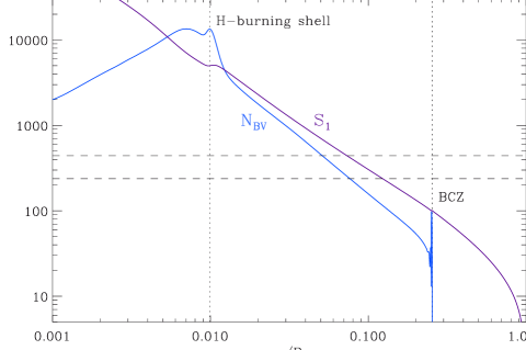
Figure 1: Brunt-Väisälä and Lamb frequency profiles for a 1.3-$M_{\odot}$ stellar model on the RGB, corresponding to model M1 of Belkacem et al. (2015) (see also Table 3). The horizontal dashed lines delimit the frequency range where oscillations are expected, around $\nu_{\mathrm{max}}$; the vertical dotted lines indicate the locations of the hydrogen-burning shell and of the base of the convection zone (BCZ), respectively.

2.2 Weak coupling

In the case of weak coupling, the decay of the wave amplitude in the evanescent region ${\mathcal{E}}$ is expressed by the transmission factor defined as

$$T\equiv\exp\left(-\int_{\mathcal{E}}\kappa\,\mathrm{d}r\right),$$ (7)

and linked to the coupling factor $q$ of the asymptotic expansion (Eq. 1) by

$$q={T^{2}\over 4},$$ (8)

as computed by Shibahashi (1979) and Unno et al. (1989).

Weak coupling is ensured if the transition region between $S_{1}$ and $N_{\mathrm{BV}}$ is wide enough. Indeed, as shown by Eqs. (7) and (8), the value of $q$ in the case of weak coupling is necessarily below 1/4. Conversely, a value of $q$ above 1/4 implies that the weak-coupling approach is insufficient.

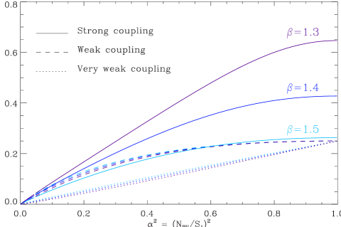
Figure 2: Relationship between the coupling factor $q$ and the ratio $\alpha^{2}=(N_{\mathrm{BV}}/S_{1})^{2}$ defined under the assumption that both frequencies have the same slope varying as $r^{-\beta}$ in the region surrounding the hydrogen-burning shell; $q$ is computed for three different values of $\beta$ (1.3, 1.4 and 1.5) in three cases: very weak (dotted lines, Eqs. 10-11), weak (dashed lines, Eqs. 7-9), or strong coupling (full lines, Eqs. 12-14). The very weak and weak coupling values hardly depend on $\beta$, unlike the strong-coupling case.

With the assumptions made in Section 2.1, so with the definitions of $\alpha$ (Eq. 6) and $\beta$ (Eq. 5), the integral term in Eq. (7) can be rewritten

$$\int_{\mathcal{E}}\kappa\ \mathrm{d}r={\sqrt{2}\over\beta}\int_{\alpha}^{1}\sqrt{1-x^{2}}\sqrt{x^{2}-\alpha^{2}}\;{\mathrm{d}x\over x^{2}},$$ (9)

where $x$ is the normalized frequency $\omega/S_{1}$. Consequently, the coupling factor depends on $\alpha$ and $\beta$ only, but does not vary in the frequency range where modes are observed. Although the evanescent region is probed at different depths by the different mixed modes, the wave transmissions through the barrier, hence $q$, are the same for each frequency because of the parallel variations of $N_{\mathrm{BV}}$ and $S_{1}$. This result confirms that $q$ is directly related to the interior structure properties (Fig. 2).

In the case of very weak coupling, the influence of the turning points can be neglected in Eq. (7). In practice, we consider that $S_{1}\gg\omega\gg N_{\mathrm{BV}}$ almost everywhere between the boundaries of the evanescent region $r_{1}$ and $r_{2}$, so that $q$ reduces to a simple function of these boundaries

$$q\simeq{1\over 4}\left({r_{1}\over r_{2}}\right)^{2\sqrt{2}}.$$ (10)

Combined with the assumption on the variations of $N_{\mathrm{BV}}$ and $S_{1}$, it can be rewritten in terms of the coefficients $\alpha$ and $\beta$:

$$q\simeq{1\over 4}\ \alpha^{2\sqrt{2}/\beta}.$$ (11)

This simplified relation shows again that $q$ does not vary in frequency range where mixed modes are observed. It also proves that $q$ provides another diagnostic parameter of red giants, complementary to the period spacing $\Delta\Pi_{1}$ that probes the Brunt-Väisälä cavity.

2.3 Strong coupling

In the strong coupling case studied by Takata (2016), the expression of the transmission $T$ is not as simple as Eq. (7) and must be replaced by a more precise expression. The relation between $q$ and $T$ becomes

$$T^{2}={4q\over(1+q)^{2}}.$$ (12)

The factor $q$ is connected to interior structure properties in the general case

$$q={1-\sqrt{1-\exp(-2\pi X)}\over 1+\sqrt{1-\exp(-2\pi X)}},$$ (13)

following Eq. (133) of Takata (2016). The new variable $X$ defined by Eq. (61) of this paper expresses

$$X\propto\int_{\mathcal{E}}\kappa\,\mathrm{d}r+X_{\mathrm{R}},$$ (14)

where the additional term $X_{\mathrm{R}}$ is important only when the frequencies $N_{\mathrm{BV}}$ and $S_{1}$ are very close to each other. It comes from the gradient of $N_{\mathrm{BV}}$ and $S_{1}$ in the evanescent region. In practice, it takes the reflection of the wave at the boundaries into account and so explains that the transmission cannot be equal to unity even when $N_{\mathrm{BV}}$ and $S_{1}$ have very close values. As a result, a very narrow evanescent region characterized by $\alpha\simeq 1$ is not associated with a coupling factor close to one.

The variation of $X$ and the relation between $X$ and $q$ make it possible to have values of $q$ significantly above the limit of 1/4 fixed by the weak-coupling case (Eq. 8). Under the assumption that $N_{\mathrm{BV}}$ and $S_{1}$ show similar radial variations, the computation of $X$, hence $q$, depends on $\alpha$ and $\beta$ only. The variation of $q$ with $\alpha^{2}$ are shown in Fig. 2, computed with Eq. (A80) of Takata (2016). This equation takes into account the perturbation of the gravitational potential that modifies the values of $N_{\mathrm{BV}}$ and $S_{1}$. The comparison of the weak and strong coupling also shows that the use of the weak-coupling case is relevant for very small values of $q$ only.

We note that, the lower the $\beta$, the larger the correction on $q$ in the strong-coupling case. Moreover, the observations of $q$ values larger than 1/4 are associated to $\beta$ values less than 1.5. We also note that the correction increases when $\alpha$ increases.

As in the weak-coupling case, $q$ does not show variation in the frequency range where modes are observed. This is the consequence of parallel variations of $N_{\mathrm{BV}}$ and $S_{1}$. In the following, we consider that the variation of $q$ with frequency is small enough, so that fitting the whole mixed-mode spectrum with a fixed coupling factor makes sense.

3 Method

In previous work (Mosser et al. 2012b, 2014), coupling factors in red giants were derived from the fit of the oscillation pattern. This fitting method, even if made precise and easy with the new view exposed in Mosser et al. (2015), cannot be automated, so that we have to provide a new method for dealing with the amount of Kepler data.

3.1 Correlations between mixed-mode parameters

The method of Vrard et al. (2016) developed for measuring the period spacing $\Delta\Pi_{1}$ offers an efficient basis for obtaining a relevant measure of $q$. According to Eq. (1), the measurements of the mixed-mode parameters $q$ and $\Delta\Pi_{1}$ are a priori independent: $\Delta\Pi_{1}$ measures the period spacings between the mixed modes whereas $q$ measures the deformation of these spacings close to the pure pressure modes (see, e.g., Fig. 2 of Vrard et al. 2016). When buoyancy glitches, rotational splittings, or simply noise, modify locally the frequency interval between two consecutive mixed modes, this independence is however not ensured. In fact, they introduce a crosstalk between the determination of $q$ and $\Delta\Pi_{1}$, which induces spurious fluctuations of $q$ when computing $\Delta\Pi_{1}$. Vrard et al. (2016), who considered $q$ as a free parameter when measuring period spacings $\Delta\Pi_{1}$, obtained $q$ with large uncertainties. In order to get $q$ in a robust manner, we had first to circumvent this crosstalk. To do so, we chose to measure $q$ and $\Delta\Pi_{1}$ in an independent manner. For measuring $q$, we considered first $\Delta\Pi_{1}$ as a fixed parameter, adopting the values of Vrard et al. (2016).

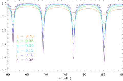
Figure 3: Variation of the stretching function $\zeta$ with $q$. The locations of the local minima of $\zeta$, which correspond to the expected pure pressure modes, do not depend on the value of $q$.

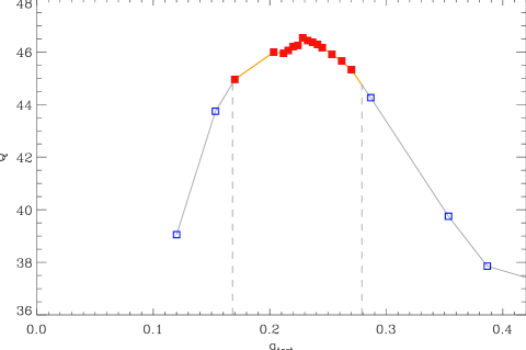
Figure 4: Variation of the signal $Q$ with the coupling factor $q_{\mathrm{test}}$ used in the stretching function $\zeta$ considered as a free parameter, for a typical clump star (KIC 1717994). The region with maximum $Q$ values (full symbols) is used to define the optimum value of $q$ and the associated uncertainty $\delta q$. The dotted lines delimit the range $q\pm\delta q$.

3.2 Measuring $q$

In practice, the first step of the method consists in a stretching of the power spectrum $P(\nu)$ by using the change of variable introduced by Mosser et al. (2015). The frequency $\nu$ is replaced by the stretched period $\tau$ according to

$$\mathrm{d}\tau={1\over\zeta}{\mathrm{d}\nu\over\nu^{2}},$$ (15)

where the function $\zeta$ is obtained from the interpolation of the values obtained for the dipole mixed-mode frequencies $\nu_{\mathrm{m}}$,

$$\zeta(\nu_{\mathrm{m}})=\left[1+{1\over q}{\nu_{\mathrm{m}}^{2}\Delta\Pi_{1}\over\Delta\nu_{\mathrm{p}}}{\cos^{2}\theta_{\mathrm{g}}\over\cos^{2}\theta_{\mathrm{p}}}\right]^{-1}.$$ (16)

The way to obtain a precise continuous function of $\zeta$ is explained by Mosser et al. (2015). It importantly depends on the correct location of the pure dipole modes, carried out by the use of the red giant universal pattern (Mosser et al. 2011b; Corsaro et al. 2012).

The power spectrum $P(\tau)$ expressed as a function of the stretched period $\tau$ is composed of $\mathcal{M}$ blended comb-like patterns, where $\mathcal{M}$ is the number of visible azimuthal orders. For a star seen equator-on, $\mathcal{M}=2$, only 1 when the star is seen pole-on, and 3 in the intermediate case.

The regularity of the $\mathcal{M}$ comb(s) is optimized when the value of $\zeta$ used for stretching the spectrum matches the correct coupling (Fig. 3). So, we varied the coupling factor $q_{\mathrm{test}}$ to obtain a varying correction $\zeta$ and searched to optimize the regularity of the comb. The optimum signal is inferred from the maximum of the Fourier transform of $P(\tau)$, noted $Q$ (Fig. 4). As is clear from Fig. 3, the regularization is only slightly affected by $q$, so that the measurement is possible for high signal-to-noise spectra only.

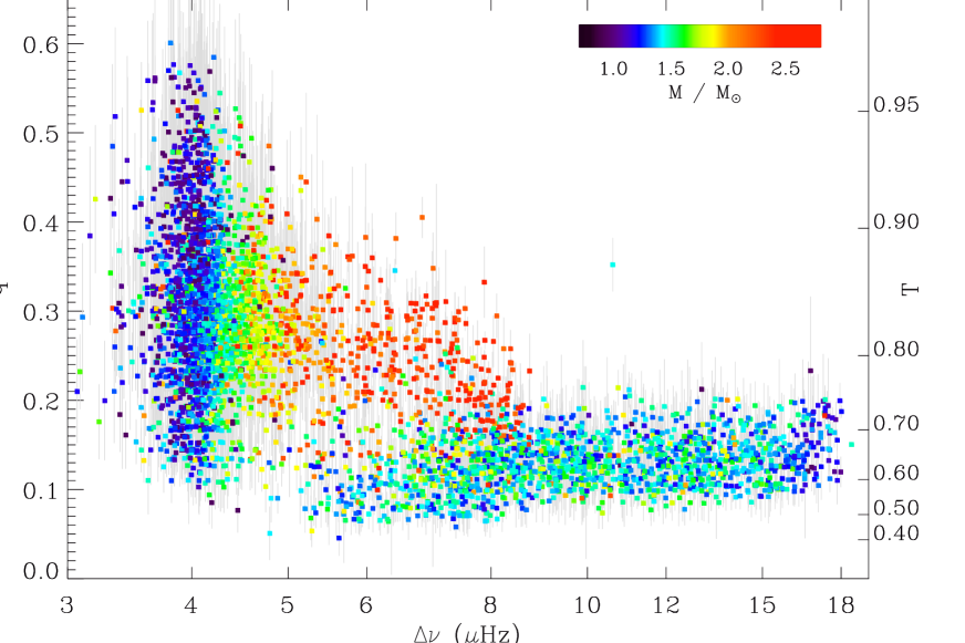
Figure 5: Coupling factor $q$ as a function of the large separation $\Delta\nu$. Asymptotic values of $\Delta\nu$ and $\Delta\Pi_{1}$ come from Vrard et al. (2016). The color codes the mass, determined with seismic scaling relations. The right vertical axis provides the corresponding values of the transmission factor $T$.

3.3 Individual check and limitations

The robustness of the method was verified with individual checks based on typical red giant oscillation spectra observed at various evolutionary stages. This check first allowed us to verify that more than 96 % of the prior values of $\Delta\Pi_{1}$ automatically measured by Vrard et al. (2016) are safe. Wrong initial values of $\Delta\Pi_{1}$ were identified by spurious measures of $q$. For oscillation spectra with a low signal-to-noise ratio, measuring the period spacing $\Delta\Pi_{1}$ still remains possible, but identifying the small variations due to the coupling is demanding. For high signal-to-noise ratio oscillation spectra, we identified three major cases providing us with incorrect measurements for $q$: pressure glitches, buoyancy glitches, and rotation. All these effects perturb the regularity of the function $\zeta$.

3.3.1 Pressure glitches

Pressure glitches occur when rapid variations of the sound speed modify the regularity of pressure modes. They contribute by adding a small modulation to the pressure mode pattern. The shift remains less than 2 % of $\Delta\nu$, as measured in the radial modes of a large set of red giants by Vrard et al. (2015). The modulation of the pure dipole pressure modes is similar to that of radial modes, so that the location of pressure-dominated mixed modes are shifted. As a result, the local minima of the stretching function $\zeta$ are shifted (Fig. 7 of Mosser et al. 2015). This change may induce variation of $Q$ larger than the variation due to $q$, so that the method fails. More importantly, the method often produced very low or very large spurious values of $q$ in that case.

3.3.2 Buoyancy glitches

Buoyancy glitches occur when rapid variations of the Brunt-Väisälä frequency modify the regularity of the gravity-mode pattern. This effect was theoretically investigated by Cunha et al. (2015). It affects mixed modes since it modifies locally the period of the stretched spectrum, with a clear signature on the function $\zeta$ (Figs. 8 and 10 of Mosser et al. 2015). Measuring a mean period spacing in the presence of buoyancy glitches is often possible, but measuring its optimization for deriving $q$ is more challenging, since variations of the period spacings due to the buoyancy glitch mimic variations due to an inadequate value of $q$. This situation most often occurs for red clump stars and may explain part of the large spread of $q$ observed for these stars.

3.3.3 Rotational splittings

Rotational splittings also perturb the measurements of $q$. In the case of low rotation (Mosser et al. 2012a), each family of stretched peaks associated to a given azimuthal order $m$ provides a comb spectrum with a period close to $\Delta\Pi_{1}$ (Fig. 6 of Mosser et al. 2015), so that the identification of $\Delta\Pi_{1}$ and of $q$ derives clearly from the optimization of the Fourier analysis of $P(\tau)$. However, the signature of the period spacings between the different peaks with different azimuthal orders sometimes dominates and hampers the measurement of $q$. This most often appears on the RGB, when the rotational splittings of the largest peaks near $\nu_{\mathrm{max}}$ are comparable to a simple fraction of the frequency differences between two consecutive mixed modes.

Individual checks based on the fit of the mixed-mode pattern and on échelle diagrams were performed on 5 % of the target to correct spurious values.

3.4 Threshold and uncertainties

The examination of various stars at different evolutionary stages allowed us to define a relevant threshold value $Q\geq 25$ characterizing a reliable measurement of $q$. Since we noticed that very low or very high values of $q$ are artefacts, we introduced a penalty function for those values. Uncertainties were empirically derived from the examination of the power spectrum $Q$ of the stretched spectrum $P(\tau)$ and by comparison with individual fittings. Variations of $Q$ less than 4 % of the maximum value were used to derive an estimate of the uncertainties $\delta q$ (Fig. 4). This is a conservative value.

We are aware that a more sophisticated statistical analysis is desirable for deriving stronger estimates of the uncertainties on $q$, as recently done by Buysschaert et al. (2016). They chose three bright stars seen pole-on, so with a high signal-to-noise ratio oscillation pattern free of any rotational splitting. Despite these favorable conditions, their analysis was computationally very demanding (Buysschaert, personal communication). An analysis aiming at measuring precise uncertainties for a large set of stars is beyond the scope of our work, which is mainly intended to provide a coherent view on a large set of stars.

4 Results

4.1 Data set

We used the data of Vrard et al. (2016), namely a catalog of about 6 100 red giants with measured period spacings and duly identified evolutionary stages. We also considered 33 subgiants, defined as subgiants according to the seismic criterion $(\Delta\nu/36.5\,\mu\hbox{Hz})(\Delta\Pi_{1}/126\,\hbox{s})>1$ introduced by Mosser et al. (2014). This latter work also provided us with the criteria necessary to identify the other evolutionary stages (RGB and clump stars). Stellar masses were estimated with the method of Mosser et al. (2013b), which uses the homology of red giant oscillation spectra to lower the uncertainties induced by pressure glitches that are present at all evolutionary stages (Vrard et al. 2015). This procedure benefits from a calibration on a large set of stars and has proved to be less biased than similar methods calibrated on the Sun only. The calibration does not depend on the evolutionary stage, which can lower its precision (Miglio et al. 2012). Recent studies all converge to state that seismic masses are slightly overestimated by about 5 – 15 % (e.g., Epstein et al. 2014; Lagarde et al. 2015; Gaulme et al. 2016); such a result does not invalidate the relevance of the seismic estimate.

4.2 Iterations for the RGB and the red clump

An iteration process allowed us to correct values of $q$ affected by an initial incorrect estimate of $\Delta\Pi_{1}$. Finally, we obtained $5200$ values of $q$, corresponding to a maximum $Q$ value larger than $25$. High-quality values characterized by $Q\geq 50$ were obtained for about 3700 stars. Results are shown in Fig. 5, where the RGB and clump stars can be easily identified since they show different variations with stellar evolution. The mass dependence visible in Fig. 5 is a consequence of the evolution dependence, so that its study requires some care (see Section 5).

The mean value of $q$ on the RGB decreases with stellar evolution from 0.18 to 0.12. Coupling factors in the red clump are most often in the range [0.2 – 0.45], with a mean value of about 0.32; more than 70 % of the red-clump values are above 1/4. This indicates that weak coupling (Eq. 8) does not hold at this evolutionary stage. For interpreting observed coupling factors of clump stars, a theoretical study of strong coupling must be considered (Takata 2016).

When the threshold level of the detection is increased, the spread in $q$ decreases for clump stars. We observed that low $Q$ values are often associated to non-evenly spaced period spectra, regardless of the signal-to-noise ratio of photometric time series. As a result, low or high $q$ values are most often related to buoyancy glitches, as observed in Mosser et al. (2015).

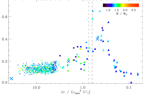
Figure 6: Coupling factor $q$ as a function of the mixed-mode density ${\mathcal{N}}=\Delta\nu/(\Delta\Pi_{1}\ \nu_{\mathrm{max}}^{2})$. The vertical dashed lines indicate the transition from subgiants to red giants defined by Mosser et al. (2014). Triangles stand for subgiants; squares for stars on the RGB (small squares for long-cadence Kepler data, big squares for short-cadence data). Three values of $q$ obtained for a synthetic 1.3-$M_{\odot}$ evolutionary sequence are also shown with $\large\times$ (see Section 5.3 and Table 3).

4.3 Subgiants

Subgiants were also considered. In that case, coupling factors were not measured with the aforementioned method, but directly determined from the fit of the mixed-mode pattern. The validity of the asymptotic expression is questionable for mixed modes with low-radial gravity orders observed in red giants. It however provides period spacings that fully agree with modelled values (Benomar et al. 2013, 2014; Deheuvels et al. 2014). In fact, even if the density of gravity modes expressed by the number ${\mathcal{N}}=\Delta\nu/(\nu_{\mathrm{max}}^{2}\Delta\Pi_{1})$ is small, the distribution of the period spacings is well reproduced by the asymptotic expression and is sensitive to $q$. From the quality of the fit of the mixed mode, we could measure this parameter and estimate relative uncertainties smaller than 20 %. The identification of high $q$ values is especially clear: in such cases, the period spacings hardly depend on the nature of the mixed mode (Fig. 3). In Fig. 6, $q$ is plotted as a function of the mixed-mode density ${\mathcal{N}}$ instead of $\Delta\nu$, in order to emphasize the change of physics when a subgiant evolves into a red giant. The strongest values of $q$, close to unity, are obtained at the transition from subgiants to red giants.

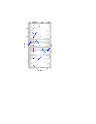
Figure 7: Échelle diagram of the very low metallicity RGB star KIC 4671239, with the stretched period $\tau$ modulo $\Delta\Pi_{1}$ on the x-axis and frequency on the y-axis. All dark symbols are dipole modes with a height above 5 times the local stellar background; their sizes depend on the mode height. When the azimuthal order can be automatically identified, triangles correspond to $m=-1$, squares to $m=0$, diamonds to $m=+1$. Light grey symbols correspond to unidentified modes: most of them are located in the region of pressure-dominated mixed modes; a few of them may also be $\ell=3$ modes. All components of the rotational multiplets intersect at 112 $\mu$Hz; the $m=\pm 1$ components intersect at 91 $\mu$Hz. The oscillation spectrum is plotted in gray top to bottom in the background of the figure in order to link the stretched periods and the mixed mode frequency.

4.4 Outliers

A limited number of stars have coupling factors significantly different from the mean behavior. We stress that their identification in this work dedicated to ensemble asteroseismology is certainly incomplete; outliers are however rare. The ones we have identified deserve future care.

4.4.1 KIC 4671239

KIC 4671239 has been identified by Thygesen et al. (2012) as one of the less metallic red giants observed by Kepler, with [Fe/H]$=-2.45$ and $T_{\mathrm{eff}}=4900$ K. Its seismic parameters are highly atypical. Apart from the high coupling value for an RGB star at a similar evolutionary stage ($q\simeq 0.25$ instead of less than 0.15), the analysis of its mixed-mode pattern has revealed a period spacing $\Delta\Pi_{1}\simeq 66.6$ s, much smaller than for RGB stars with similar $\Delta\nu$ (Mosser et al. 2014; Vrard et al. 2016), and a much higher core rotation (Mosser et al. 2012a) with $\delta\nu_{\mathrm{rot}}\simeq 830$ nHz. These parameters translate in a complex mixed-mode pattern where the different azimuthal orders show intricate structures. Disentangling this pattern is possible only with an échelle diagram constructed with stretched periods (Fig. 7), following Mosser et al. (2015) and Gehan et al. (2016).

4.4.2 KIC 6975038

KIC 6975038 also shows atypical seismic parameters, with $\Delta\Pi_{1}\simeq 57.9$ s, much smaller than comparable stars with $\Delta\nu=10.61\,\mu$Hz, and $q\simeq 0.35$, much above the values observed on the RGB. We note that the low value of $\Delta\Pi_{1}$ and the high value of $q$ may both indicate a larger radiative cavity, hence a smaller region where modes are evanescent, than in other stars with similar $\Delta\nu$.

4.4.3 Massive stars

Stars in the secondary clump, more massive than 1.8 $M_{\odot}$, show lower $q$ compared to less massive stars burning their core-helium. The difficulty to fit their mixed-mode spectrum does not resemble to the difficulty met in presence of buoyancy glitches (Mosser et al. 2015). A better fit of the data can be obtained with a gradient in $q$ as a function of frequency. According to the study conducted in Section 2, this gradient may result from the fact that the $N_{\mathrm{BV}}$ and $S_{1}$ profiles are not parallel in the evanescent region of such stars.

This effect appears for stars as KIC 4372082 or 6878041, more massive than the secondary-clump stars studied by Deheuvels et al. (2015). Such objects are rare and, despite low-quality spectra, certainly deserve detailed study and modelling.

5 Discussion

The variation of the coupling factor with the large separation $\Delta\nu$ can be used to derive direct information on the extent of the evanescent region between the $N_{\mathrm{BV}}$ and $S_{1}$ profiles, with the formalism introduced in Section 2. Even if mixed modes probe these functions in a limited frequency range around $\nu_{\mathrm{max}}$, the hypothesis that the $N_{\mathrm{BV}}$ and $S_{1}$ profiles are parallel in the considered region helps us in deriving precise information on stellar interior properties, regardless of the consequence of the decrease of $\nu_{\mathrm{max}}$ with evolution. The hypothesis is finally discussed in Section 5.4.

5.1 Variation with the evolutionary stage

5.1.1 Subgiant - red giant transition

Mosser et al. (2014) have shown that the transition between subgiants and redgiants has a clear signature in the $\Delta\Pi_{1}$ – $\Delta\nu$ diagram. In the subgiant phase, the relation between these asymptotic period and frequency spacings shows a large spread with a significant mass dependence, whereas the parameters are tightly bound on the RGB. The coupling factor $q$ is similarly impacted by the evolution and shows a significant increase at the end of the subgiant phase (Fig. 6). This increase occurs in parallel with the first dredge-up, when the base of the convection zone goes deeper in the envelope. A large value of $q$ indicates that not only the $N_{\mathrm{BV}}$ profile but also the $S_{1}$ profile is deep in the stellar interior. Observing high values in the range [0.40 – 0.65] near the transition region from subgiants to red giants argues, using Fig. 2, for a slope $\beta$ slightly higher than or close to 1.3 with a ratio $\alpha^{2}$ larger than about 0.5.

Table 1: Mass dependence of $q$ on the RGB

$M/M_{\odot}$	1.0	1.2	1.4	1.6	1.8	2.0
$q_{M}$	0.144	0.128	0.126	0.123	0.134	0.134
$\sigma_{q}$	0.021	0.025	0.026	0.022	0.023	0.027

The variation of $q$ with $\Delta\nu$ is modelled as $q=q_{M}(\Delta\nu/10)^{0.096}$, with $\Delta\nu$ in $\mu$Hz.

Table 2: Mass dependence of $q$ in the red clump

$M/M_{\odot}$	0.9	1.1	1.3	1.5	1.7	2.0
$q_{\mathrm{b}}$		0.301	0.287	0.274	0.272
$\bar{q}$	0.363	0.324	0.299	0.289	0.283	0.270
$q_{\mathrm{e}}$		0.339	0.313	0.303	0.290
$\sigma_{q}$	0.024	0.016	0.011	0.010	0.012	0.022

$q_{\mathrm{b}}$, $\bar{q}$ and $q_{\mathrm{e}}$ measure the coupling for respectively the early, middle and late stages in the clump, defined in Mosser et al. (2014); these values are defined by 25 % of the stars lying on the first, middle, and late portion of the mass-dependent evolutionary track, respectively; $\sigma_{q}$ measures the spread of the values; the fits were derived from high-quality spectra with $Q\geq 50$.

5.1.2 On the RGB

At the beginning of the ascent on the RGB, the stellar core contracts and the envelope expands. The decrease of $q$ means either that the region between $N_{\mathrm{BV}}$ and $S_{1}$ expands too, inducing a decrease of $\alpha$, or that the coefficient $\beta$ increases toward the value 3/2. A simultaneous variation of both terms $\alpha$ and $\beta$ is possible too.

For evolved models on the RGB, $\nu_{\mathrm{max}}$ becomes smaller than the value of $N_{\mathrm{BV}}$ at the base of the convective zone, so that the hypothesis of parallel variations of $N_{\mathrm{BV}}$ and $S_{1}$ is no longer valid for evolved stars on the RGB (e.g., Montalbán et al. 2013). In fact, the decrease of $q$ with stellar evolution can result either from the decrease of $\nu_{\mathrm{max}}$ or from the expansion of the region between $N_{\mathrm{BV}}$ and $S_{1}$, so that it is impossible to derive any firm conclusion in terms of interior structure evolution.

The decrease of $q$ on the RGB plays a non-negligible role in the difficulty to observe mixed modes at small $\Delta\nu$ predicted for high- and low-mass stars (Dupret et al. 2009; Grosjean et al. 2014). In fact, mixed modes that are not in the close vicinity of the pressure-dominated modes are poorly coupled, so that they show an important gravity character, hence a high inertia and a tiny amplitude. In practice, measuring low values of $q$ is hard.

In order to estimate the mass dependence of $q$ observed on the RGB, we first fitted the slope of $q(\Delta\nu)$ as a power law, under the assumption that the exponent does not depend on the stellar mass. In a second step, we quantified the mass dependence in the relation $q(\Delta\nu)$. For low-mass stars with a degenerate helium core, the higher $M$, the lower $q$; for stars more massive than 1.8 $M_{\odot}$, the situation is inverted (Table 1). This change occurs near the limit in mass between the red and secondary clumps, so is likely related to the degeneracy of helium in the core.

5.1.3 In the red clump

In the red clump, the mass dependance of $q$ is coupled to the large separation dependence: the lower the mass, the higher the coupling. This behavior is discussed in the next paragraph, since it obeys to a general trend in the relationship between $q$ and $\Delta\Pi_{1}$.

Mean values of the coupling for red clump stars are given in Table 2. Using the seismic evolutionary tracks depicted in Mosser et al. (2014), we could measure the evolution of $q$ in the red clump, at fixed mass. Values at the early, middle and late stages in the clump are shown in Table 2. As shown by Mosser et al. (2015), the evolution of stars in the red clump show non-monotonous variation of both $\Delta\nu$ and $\Delta\Pi_{1}$. Conversely, the monotonous increase of $q$ indicates either that the ratio $\alpha$ increases along the evolution of low-mass stars in the red clump, resulting from a small shrinking of the evanescent region, or that the exponent $\beta$ decreases. Both effects may simultaneously contribute to the variations.

5.2 Variation with the period spacing

The variations of $q$ with the period spacing $\Delta\Pi_{1}$ depend on the evolutionary stage. Either on the RGB or in the clump, the global variations of $q(\Delta\Pi_{1})$ indicate that the larger $\Delta\Pi_{1}$, the larger $q$ (Fig. 8). A large value of $\Delta\Pi_{1}$ is representative of a small dense core with high $N_{\mathrm{BV}}$ values. So, we come to the conclusion that high values of $N_{\mathrm{BV}}$ and $S_{1}$ occur in similar situations, and that they get close to each other when they increase together. At fixed $\beta$, the ratio $\alpha=N_{\mathrm{BV}}/S_{1}$ is then correlated with $\Delta\Pi_{1}$ for both RGB and clump stars (but not for subgiants).

Since the variations of $q$ are nearly linear in both domains, simple fits can be used as proxies for $q$ (Fig. 8):

$$q_{\mathrm{RGB}} = -0.0034+{\Delta\Pi_{1}\over 597},$$ (17)

$$q_{\mathrm{clump}} = 0.082+{\Delta\Pi_{1}\over 1450},$$ (18)

where $\Delta\Pi_{1}$ is measured in seconds. The fit of $q_{\mathrm{RGB}}$ is however not efficient for early RGB stars; the fit of $q_{\mathrm{clump}}$ is valid for both primary and secondary clumps. Such fits are intended to facilitate the identification of the mixed-mode pattern, not for explaining the physics of the coupling.

Table 3: Seismic properties of 1.3 $M_{\odot}$ models

Model	Evol.	Age	$\nu_{\mathrm{max}}$	$\Delta\nu$	$\Delta\Pi_{1}$	$q$
	stage	(Gyr)	($\mu$Hz)	($\mu$Hz)	(s)
M0	subgiant	4.40	670	39.5	182	0.40
M1	RGB	4.59	341	22.9	97	0.20
M2	RGB	4.79	49.0	5.24	63	0.045

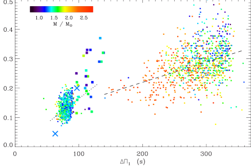
Figure 8: Coupling factor $q$ as a function of the period spacing $\Delta\Pi_{1}$ for RGB and clump stars. Same symbols as in Fig. 6. A threshold at $Q=100$ reduces the number of stars compared to Fig. 5. The dotted and dashed lines correspond to the fits for RGB and clump stars, respectively.

5.3 Modelling and computation of $q$

We used stellar models to match the observed coupling factor. We considered 1.3-$M_{\odot}$ models at three evolutionary stages (Table 3), without overshoot or diffusion; their full description is given in Belkacem et al. (2015). In the strong coupling case (model M0), we computed $q$ from Eqs. (12)–(14) using the asymptotic formalism of Takata (2016) and taking the perturbation of the gravitational potential into account. In the intermediate case (model M1), using a similar analysis is questionable since hypotheses in the calculation of $X_{\mathrm{R}}$ are valid when the evanescent region is very thin. Nevertheless, the strong-coupling analysis matches the weak-coupling case when the evanescent region becomes very large, so that we computed $q$ in a similar way as for the model M0. In the weak coupling case (model M2), we used the same expression, but with $X_{\mathrm{R}}=0$, and finally compare these three factors with observations. They show in fact small variations with frequency, so that we had to consider their mean value, defined in a 4-$\Delta\nu$ broad frequency range centered on $\nu_{\mathrm{max}}$. We checked that the term $X_{\mathrm{R}}$ introduced by Eq. (14) significantly reduces the value of $q$ and also contributes to the relative stability of $q$ with frequency. We also noticed that the perturbation of the gravitational potential plays a non-negligible role not only in the core but also in the evanescent zone and in the inner region of the convective envelope. This provides evidence that the Cowling approximation is not appropriate for computing $q$.

Modelling quantitatively agrees with observations, except for the most evolved model. The subgiant model M0 close to the transition to red giants shows a high $q$; the next model M1 is on the RGB and has a much lower $q$. Both agree with the observed values. The coupling factor for model M2, higher on the RGB, shows however a value significantly smaller than observed. In M2, the evanescent region is in fact above the base of the convective envelope (e.g., Fig. 2 of Montalbán et al. 2013). This point deserves further work, beyond the scope of this paper.

Modelling red clump stars requires special care in the prescription of convection and mixing in the core (Lagarde et al. 2012; Bossini et al. 2015). We could not compare our results with modelling but used the calculations exposed in Section 2. The high values observed for $q$ in the clump imposes the exponent $\beta$ (Eq. 5) to be less than $3/2$ (Fig. 2).

5.4 Variation of $q$ with frequency

For a limited number of stars examined by Vrard et al. (2016), the asymptotic expansion does not provide a satisfying fit of the mixed-mode pattern, without a direct explanation in terms of buoyancy glitch. For these stars, a better fit is obtained when varying $q$ with frequency. Modelling derives similar conclusion, with different slopes $\beta_{N}$ and $\beta_{S}$ (Eq. 5) or more complicate variations (e.g., Montalbán et al. 2013).

Since the independence of $q$ with frequency derives from the hypothesis of parallel variations of $N_{\mathrm{BV}}$ and $S_{1}$, we have to conclude that this hypothesis is not fully correct. The observational study of the variations of $q$ with frequency appears to be highly challenging, for the same reasons as those explaining the difficulties in measuring $q$ (rotation, glitches and finite mode lifetimes). The individual study of bright stars with a high signal-to-noise ratio is necessary to investigate the frequency dependence of $q$ in detail. Combined with modelling, this study will help assessing to which extent the mean value of $q$ is a global seismic parameter as informative for the evanescent region as $\Delta\nu$ and $\Delta\Pi_{1}$ for the pressure and radiative cavities, respectively.

6 Conclusion

The new method setup for measuring the coupling factor of mixed modes in evolved stars has provided the first analysis of this parameter over a large set of stars. We could determine 5200 values of $q$, from subgiants to clump stars. Three main results can be inferred:

- Coupling factors test the region between the Brunt-Väisälä cavity and the $S_{1}$ profile, dominated by the radiative core and the hydrogen-burning shell. Indeed, while $\Delta\nu$ is mainly sensitive to the envelope and $\Delta\Pi_{1}$ provides the signature for the core, we can directly access the intermediate region with $q$.

- The variation of $q$ with stellar evolution provides us with new constraints on stellar modelling. We note that the coupling factors show simple global variations with the period spacing, for both RGB and clump stars. The characterization of outliers can be used to constrain physical processes inside stars.

- Strong coupling is observed in stars at the transition subgiant/red giant and in the red clump. In fact, the weak-coupling formalism of Unno et al. (1989) fails for a quantitative use of the observed coupling factors, except for the most evolved stars on the RGB. In all other cases, the use of the new formalism proposed by Takata (2016) for strong coupling is mandatory.

These measurements also open the way to more precise fits of the mixed-mode pattern, in order to analyze in detail extra features, as the rotational splittings and the buoyancy glitches.