Effect of interactions and disorder on the relaxation of two-level systems in amorphous solids

Abstract

At low temperatures the dynamical degrees of freedom in amorphous solids are tunneling two-level systems (TLSs). Concentrating on these degrees of freedom, and taking into account disorder and TLS-TLS interactions, we obtain a ”TLS-glass,” described by the random field Ising model with random $1/r^{3}$ interactions. In this paper we perform a self consistent mean field calculation, previously used to study the electron-glass (EG) model [A. Amir et al., Phys. Rev. B 77, 165207, (2008)]. Similarly to the electron-glass, we find a $\frac{1}{\lambda}$ distribution of relaxation rates $\lambda$, leading to logarithmic slow relaxation. However, with increased interactions the EG model shows slower dynamics whereas the TLS glass model shows faster dynamics. This suggests that given system specific properties, glass dynamics can be slowed down or sped up by the interactions.

I Introduction

At low temperatures amorphous solids show anomalous behavior with respect to their ordered counterparts. As was first noted by Zeller and Pohl Zeller and Pohl (1971) the equilibrium properties of amorphous solids have different temperature dependence than predicted by the Debye model; some examples are the temperature dependences of the heat capacity $c_{v}\propto T^{\alpha}$, and the thermal conductivity $\kappa\propto T^{\beta}$ where $\alpha\approx 1$ and $\beta\approx 2$. Moreover, phonon attenuation is qualitatively and quantitatively universal in a large variety of disordered and amorphous materials. Shortly after, Anderson et al. Anderson et al. (1972) and Phillips Phillips (1972) independently developed the standard tunneling model (STM), a phenomenological model which quite successfully accounts for many of the low temperature characteristics of amorphous solids. The STM states that at low temperatures the dominant dynamical degrees of freedom are two-level systems (TLSs); each TLS represents an atom or a group of atoms that occupy one of two localized configuration states that result from an asymmetric double-well potential. TLSs are defined by their asymmetry energy $\Delta$ and tunneling amplitude $\Delta_{0}\sim e^{-\Lambda}$. Given the random nature of the system, $\Delta$ and $\Lambda$ are assumed to be distributed uniformly leading to the distribution $P(\Delta,\Delta_{0})=\frac{P_{0}}{\Delta_{0}}$Anderson et al. (1972); Phillips (1972, 1987). TLSs reach thermal equilibrium with the phonon bath through a linear coupling to the local strain. Whereas in its basic form the STM considers noninteracting TLSs, TLSs interact via acoustic and electric dipole interactions. TLS-TLS interactions result in, e.g., spectral diffusion Black and Halperin (1977), delocalization of low energy pair excitations Burin and Kagan (1994), and slow relaxation of dielectric and acoustic response at very low temperatures Rogge et al. (1996); Natelson et al. (1998) suggesting the formation of a TLS-glass (TG).

Recent work on microfabricated devices caused a renewed interest in TLSs, both for harnessing them for technological applications, for example quantum memory Neeley et al. (2008), and for avoiding their destructive influence as a source of noise. In particular, superconducting quantum bits (qubits) have shown extreme sensitivity to even a single TLS Simmonds et al. (2004); Barends et al. (2014). This coupling of the qubit system to TLSs was then used to investigate the characteristics of individual TLSs Neeley et al. (2008); Shalibo et al. (2010); Lisenfeld et al. (2016); Matityahu et al. (2016) and specifically the nature of TLS-TLS interactions up to the accuracy of a single interacting pair Lisenfeld et al. (2015).

The thermodynamic and the dynamic properties of single non-interacting TLSs have been studied thoroughly Anderson et al. (1972); Phillips (1987); Lisenfeld et al. (2010); Grabovskij et al. (2012); Müller et al. (2015); Matityahu et al. (2016). The many-body dynamics of interacting TLSs is, however, more complicated. It was studied e.g. with regard to the relaxation of the dielectric response of the interacting TLSs system Burin (1995); Rogge et al. (1996); Natelson et al. (1998); Burin et al. (1998) and to the relaxation and decoherence of resonant TLS pairs Burin and Kagan (1994, 1996). In this paper we are interested in the relaxation dynamics of the occupations of the interacting TLS-glass in a large parameter regimes, and in its dependence on the strength of the interaction, strength of disorder, and system size.

To obtain the relaxation dynamics of the TLS glass we follow a similar method to that used previously for the electron-glass (EG) modelAmir et al. (2008). We calculate numerically the density of states of the interacting TLS system in the mean-field approximation and use it to determine the TLS-phonon transition rates. The total relaxation of the system is then calculated by taking the norm of the occupation vector, which is the solution of the linearized Pauli rate equation. Taking the rates to the continuum and using the $1/\lambda$ distribution of rates the logarithmic slow relaxation is obtained. Furthermore, the logarithm depends on interactions and disorder through the minimum cutoff rate, $\lambda_{min}$. Using this dependence we examine the qualitative effect of the interactions, disorder and systems size on the dynamics, and compare it with the EG model.

The structure of the paper is as follows: In Sec. II we define the local-equilibrium state of the system, present the model in the mean-field approximation and obtain numerically the single particle density of states (DOS) which contains the dipole gap. In Sec. III, we derive the logarithmic shape of the relaxation. In Sec. IV we show the numerical results of the DOS and the distribution of rates for different values of the disorder and interaction. In Sec. V we compare our results to the results of the EG model under the same schemes of parameter variation, and discuss the dependence of the relaxation on the system size for both the EG and TLS models. We then conclude in Sec. VI.

II The TLS-Glass model

In this section we discuss the STM model the with addition of Ising type interactions between the TLSs. We then apply the mean-field (MF) approximation and obtain the self-consistent equations.

We consider the Hamiltonian

$$\begin{split}\mathcal{H}_{TG}=&\sum_{i}\left(\Delta_{i}S^{z}_{i}+\Delta_{0i}S^{x}_{i}\right)-\frac{1}{2}\sum_{i\neq j}\frac{u_{ij}}{r^{3}_{ij}}S^{z}_{i}S^{z}_{j}\,,\\ \end{split}$$ (1)

where $S^{z(x)}=\frac{1}{2}\sigma^{z(x)}$ represent the TLSs ($\sigma^{z(x)}$ are the Pauli matrices). $J_{ij}=\frac{u_{ij}}{r_{ij}^{3}}$ represents both acoustic and electric interactions between TLSs. Since both interactions depend on the orientations and relative positions of the two TLSs, we choose $u_{ij}$ from a random Gaussian distribution.

$$p(u)=\frac{1}{\sqrt{2\pi}U_{0}}\exp\left(-\frac{1}{2}\frac{u^{2}}{U_{0}^{2}}\right)\,,$$ (2)

and quantify the interaction strength by $J\equiv U_{0}/r^{3}_{nn}$, where $r_{nn}$ is the average nearest-neighbor distance. Numerically we set $r_{nn}=1$.

To obtain the MF energies one can apply on $\mathcal{H}_{TG}$, Eq. (1), a variational derivative with respect to $S^{z}_{i}$ and obtain the MF asymmetry energy $\Delta^{\prime}_{i}$ ,

$$\Delta^{\prime}_{i}=\frac{\delta\mathcal{H}_{TG}}{\delta S^{z}_{i}}=\Delta_{i}-\frac{1}{2}\sum^{N}_{j(\neq i)}\frac{u_{ij}}{r^{3}_{ij}}S^{z}_{j}$$ (3)

where $\Delta_{i}$ is the asymmetry energy of TLS $i$. $\Delta_{i}$ is chosen from a Gaussian distribution with variance $W$, which we use to quantify the disorder. $N$ is the number of sites (system size).

After thermal averaging the obtained self-consistent equation (SCE) is:

$$\Delta^{\prime}_{i}=\Delta_{i}+\frac{1}{4}\sum_{j\neq i}\frac{u_{ij}}{r^{3}_{ij}}\tanh\left(\frac{\Delta^{\prime}_{j}}{2T}\right)$$ (4)

where we set the Boltzmann constant to unity, reassign $\Delta^{\prime}_{i}=\langle\Delta^{\prime}_{i}\rangle_{T}$, and use $\langle S^{z}_{i}\rangle_{T}=\frac{1}{2}\langle\sigma^{z}_{i}\rangle_{T}=-\frac{1}{2}\tanh\left(\frac{1}{2}\beta\Delta^{\prime}_{i}\right)$. The single TLS shifted Hamiltonian is:

$$\mathcal{H}^{\prime}_{TLS}=\sum_{i}\left(\Delta^{\prime}_{i}S^{z}_{i}+\Delta_{0i}S^{x}_{i}\right)$$ (5)

and the equilibrium excitation energy of the $i$’th TLS is:

$$E_{i}=\text{sgn}(\Delta^{\prime}_{i})\sqrt{{\Delta^{\prime}_{i}}^{2}+\Delta^{2}_{0i}}$$ (6)

Unlike the distribution given in the STM, $p(\Delta,\Delta_{0})=\frac{P_{0}}{\Delta_{0}}$, which is uniform in the asymmetry energies, we choose

$$p\left(\Delta,\Delta_{0}\right)=\frac{P_{0}}{\Delta_{0}}\frac{1}{\sqrt{2\pi}W^{2}}\exp\left(-\frac{1}{2}\frac{\Delta^{2}}{W^{2}}\right)\,.$$ (7)

This choice eventually does not affect the qualitative physical outcome. However, it allows us to look at the effect of changing disorder. It is also in line with the DOS of the asymmetry energies for the relevant TLSs at low energies in KBR:CN (CN flips)Churkin et al. (2014), as well as in the two TLS modelSchechter and Stamp (2013); Churkin et al. (2013).

Previous work Baranovskii et al. (1980); Cuevas et al. (1989); Burin (1995) has shown that the DOS of the TG system in 3D has a logarithmic gap which results from the dipole interactions. We present the numerical solution of the self-consistent equations (Eq. (3)), which gives the same logarithmic dependence, and in addition the behavior for larger energy values far from the gap region. Note, however, that for large disorder the gap width is exponentially small in the parameter $W/J$Schechter and Stamp (2013), unlike the polynomial dependence on disorder for the EG model Efros and Shklovskii (1975). The calculation of the TG energies within mean field allows us to gain an understanding of the relation between the DOS and the dynamics of the system, and in particular its dependence on control parameters of the model such as disorder, interaction strength and system size. Following an iterative procedure done by Grunewald et al. Grunewald et al. (1982) we calculate numerically the solution of the SCE, Eq. (4), for finite temperature. We set the initial values of the MF asymmetry energy $\Delta^{\prime}_{i}$ to uniform distribution, and perform an iterative procedure that eventually converges to the solution of the SCE. We then obtain the excitation energies of the TLSs given in Eq. (6). The normalized histogram (DOS) of the energies is plotted in Fig. 1.

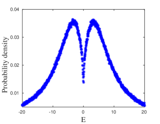
Figure 1: (Color online) TLS DOS. The normalized histogram (DOS) of TLS energies $E_{i}=\text{sgn}(\Delta^{\prime})\sqrt{{\Delta^{\prime}}_{i}^{2}+\Delta_{0i}^{2}}$ obtained by solving the self-consistent equations, Eq. (3), for $N=10000$ sites, $W=J=1,T=0.05$. Results are averaged over 300 realizations.

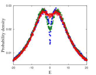
Figure 2: (Color online) TLS DOS for different temperatures. $T=0.1$ (blue asterisks), $T=1$ (green squares), and $T=2$ (red triangles) for $N=1000$. The gap gradually disappears with increasing temperature.

Furthermore, as shown numerically in Fig. 2 the gap disappears gradually as the temperature increases. A similar phenomenon occurs for the electron-glass model (as discussed in Sec. V). Note that $\Delta_{0}$’s do not evolve with the iterations since their coupling to phonons is neglected Anderson et al. (1972); Phillips (1972). In all the numerical calculations the parameters of Eq. (3) are measured in units of the interaction at average nearest-neighbor distance $J=\frac{U_{0}}{r^{3}_{nn}}$ and the TLSs are distributed homogeneously in a three dimensional cube with periodic boundary conditions. Also, $\Delta_{0}$ is taken to be in the range $[10^{-7},10^{-1}]$ Burin (1995); Anderson et al. (1972). Excluding the case where the interaction parameter, $J$, is varied explicitly, we set the tunneling strength to be $\chi\equiv P_{0}U_{0}=10^{-3}$ given the fact that it ranges between $10^{-3}$ and $10^{-4}$ in all known amorphous materials Phillips (1987).

III Dynamics

In this section we follow a similar approach to that used by Amir et al. Amir et al. (2008) for the EG, and obtain the relaxation to local equilibrium of the TG model. The dynamics of the average occupation of state $i$ at time $t$ is generally described by the Pauli master equation:

$$\frac{dp_{i}(t)}{dt}=\sum_{j\neq i}\omega_{ij}p_{j}(t)-\omega_{ji}p_{i}(t)$$ (8)

where $\omega_{ij}$ is the transition rate from state $j$ to state $i$ and the occupation $p_{i}(t)$ can take the values in the range $[0,1]$. Equation (8) conserves the total probability; i.e., $\sum_{i=1}p_{i}(t)$ is constant. Specifically for the EG, Amir et al. (2008) this reflects the conservation of the total number of electrons. However, in the TG system the transition of probability between any two TLSs is not allowed and therefore there is probability conservation for each TLS separately, $\sum_{m=1,2}p^{i}_{m}(t)=p^{i}_{1}+p^{i}_{2}=1$, where $p^{i}_{1},p^{i}_{2}$ are respectively the average probability occupations of the low energy and high energy local levels of the TLS at site $i$. Accordingly, Eq. (8) is reduced to two coupled rate equations of the occupations of the $i$’th TLS:

$$\begin{split}\frac{dp^{i}_{1}(t)}{dt}&=\omega^{i}_{-}p^{i}_{2}(t)-\omega^{i}_{+}p^{i}_{1}(t)\\ \frac{dp^{i}_{2}(t)}{dt}&=\omega^{i}_{+}p^{i}_{1}(t)-\omega^{i}_{-}p^{i}_{2}(t)\end{split}$$ (9)

where $\omega^{i}_{+}$ and $\omega^{i}_{-}$ are respectively the TLS upward and downward transition rates caused by the TLS interaction with the phonon bath $\sum_{i}\sum_{k}g_{ik}\left(a^{\dagger}_{-k}+a_{k}\right)S^{x}_{i}$, where $k$ represents phonon with momentum vector $\bm{q}$ and polarization $s$, and $g_{ik}$ is coupling constant which is proportional to the deformation potential constant $\gamma_{is}$. The rates are obtained via Fermi’s golden rule Phillips (1987):

$$\omega^{i}_{-}=\sum_{s}\frac{\gamma_{is}^{2}}{c^{5}_{s}}\frac{\Delta_{0i}^{2}E_{i}}{2\pi\rho\hbar^{4}}\left(N_{i}+1\right)\equiv a_{i}\Delta_{0i}^{2}E_{i}\left(N_{i}+1\right)$$ (10)

and a similar expressions for $\omega^{i}_{+}$, with the brackets in Eq. (10) replaced with $N_{i}$. Here $a_{i}\equiv\sum_{s}\frac{\gamma_{is}^{2}}{c^{5}_{s}2\pi\rho\hbar^{4}}\simeq 10^{8}K^{-3}s^{-1}$, where Boltzmann constant is set to unity, $N_{i}=\left(e^{\beta E_{i}}-1\right)^{-1}$ is the equilibrium phonon occupation at a given energy splitting of the TLS $(E_{i})$, and $\beta=\frac{1}{T}$ is the inverse temperature. Finally, Eq. (9) reduces to one parameter in the pseudospin representation by substituting $\sigma_{i}=\langle\sigma^{z}_{i}\rangle=p^{i}_{2}-p^{i}_{1}$:

$$\frac{d\sigma_{i}}{dt}=-2a_{i}\Delta_{0i}^{2}E_{i}\left[\sigma_{i}\left(N_{i}+\frac{1}{2}\right)+\frac{1}{2}\right]=-\lambda_{i}\sigma_{i}-a_{i}\Delta_{0i}^{2}E_{i}$$ (11)

where the TLS-phonon relaxation rate in equilibrium is Jäckle (1972); Phillips (1987)

$$\lambda_{i}=-(\omega^{i}_{-}+\omega^{i}_{+})=-a_{i}\Delta^{2}_{0i}E_{i}\coth\left(\frac{E_{i}}{2T}\right)\,.$$ (12)

Equation (11) has a simple form but has hidden complexity. The right-hand side depends on the energy $E_{i}$ which in turn depends on the interactions, disorder and out-of-equilibrium occupations of all the TLSs in the system, i.e., $E_{i}(\bm{\sigma^{\prime}})$ where $\bm{\sigma^{\prime}}$ denotes all the elements of the pseudospin vector except the $i$th element.

For TLS occupations slightly out of equilibrium ($\delta\sigma_{i}\equiv\sigma_{i}-\sigma_{i}^{0}\ll 1$) we can expand the right-hand side of Eq. (11) to first order in $\delta\sigma_{i}$ around the local equilibrium point. Neglecting a subdominant interaction termAmir et al. (2008) (see App. B for details) we obtain

$$\frac{d\delta\sigma_{i}}{dt}\simeq-\lambda_{i}\delta\sigma_{i}\,.$$ (13)

Eq. 13 has a simple solution:

$$\delta\sigma_{i}(t)=c_{i}e^{-\lambda_{i}t}$$ (14)

where $c_{i}\equiv\delta\sigma_{i}(0)$ is the initial deviation of TLS $i$ at the moment the external strain driving force has stopped. To quantify the total relaxation of the system one can take the norm of the vector $\bm{\delta\sigma}$ Amir et al. (2008):

$$|\bm{\delta\sigma}|=\sum_{i}c_{i}e^{-\lambda_{i}t}$$ (15)

and in the continuous limit,

$$|\bm{\delta\sigma}|=c\int^{\lambda_{max}}_{\lambda_{min}}p(\lambda)e^{-\lambda t}d\lambda\,$$ (16)

where a uniform distribution of initial excitations $c(\lambda)=c$ is assumedAmir et al. (2008). The rate distribution is then calculated numerically and obeys a $\frac{1}{|\lambda|}$ distribution over a very broad rate regime.

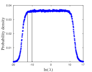
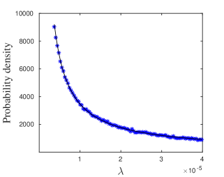
Figure 3: (Color online) Decay rate distribution for the TLS-glass. The distribution of decay rates $\lambda_{i}$ presented in Eq. (12) calculated for $N=10000$ and $\frac{J}{T}=10$. The disorder energy, tunneling splinting and interaction strength are the same as in Fig. 1. The graph is averaged over 1000 realizations. (a) Rate distribution in log scale for the full range of values. The bulk of rates occupy the plateau region which translates to $\frac{1}{\lambda}$ form in normal scale. (b) Rate distribution within the cutoff region in the log plot shown in linear scale with a $\frac{1}{\lambda}$ fit.

In Fig. 3 we plot the rates distribution using Eq. (12) and the energies given in Fig. 1. The normal scale is shown in a regime determined by a lower cutoff being the minimum value of the plateau region in the log plot, $\lambda_{min}$. This value also determines the relaxation time scale of the system (see Eq. (17) below). The maximum cutoff value $\lambda_{max}$ is fixed arbitrarily and has no significance. The $\frac{1}{|\lambda|}$ functional form of the distribution is a result of the dependence of the decay rates on $\Delta^{2}_{0}$ [see Eq. (12)] in conjunction with the joint distribution function $p(\Delta_{0},\Delta^{\prime})\propto 1/\Delta_{0}$. Finally we substitute in Eq. (16) the rate distribution and obtain the logarithmic relaxation:

$$\begin{split}|\bm{\delta\sigma}|\simeq-c\left[\gamma_{E}+log\left(\lambda_{min}t\right)\right]\end{split}$$ (17)

where $\gamma_{E}\approx 0.577$ is the Euler constant and the integral is approximated for $1/\lambda_{max}<t<1/\lambda_{min}$ Bender and Orszag (1999). The logarithmic relaxation we find here is in line with the TLS-glass being a part of a large class of materials with a similar slow logarithmic relaxation Amir et al. (2012). As mentioned above, the $\frac{1}{|\lambda|}$ functional form of the rates distribution is dominated by the distribution of $\Delta_{0}$, and is thus independent of disorder and interaction strengths. However, the latter change the density of states of single particle excitations, and specifically that at low energies, that dominate the slowest transition rates Phillips (1987). Thus, disorder and interaction can shift the distribution of relaxation rates to higher or lower values, see below.

IV Effect of interactions and disorder

In this section we study the effect of the variation of disorder and interaction on the DOS and on the dynamics of the TLS glass. In particular, we find that the interactions speed up the relaxation process rather than slow it down, in contrast to what was found for the EG model Amir et al. (2008) (see also Fig. 13 below).

IV.1 Effects of interaction and disorder on the DOS of single TLSs

We present two schemes:

1. Varying the disorder ($W$) for constant interactions ($J$) and constant $W/T$ ratio. For increasing disorder the DOS broadens and the gap diminishes (see Fig. 4). We note that a similar broadening is obtained for varying the disorder $W$ while keeping $T=0.1J$ constant.

2. Varying the the ratio $J/W$ while holding the sum of the variances constant ,$W^{2}+J^{2}=2$. This is done in order to change the strength of the interactions while not significantly affecting of the energy variance,

   $$\left<E_{i}^{2}\right>\approx W^{2}+\left<\Delta^{2}_{0i}\right>+\sum_{j}\frac{U_{0}^{2}}{r^{6}_{ij}}\left<S^{2}_{j}\right>.$$ (18)

   With the increase of the interaction strength (and decreasing of $W$) the overall effect is a broadening of the DOS and a deepening of the gap (see Fig. 5). For a similar scheme where only the interactions parameter is increased a greater broadening is obtained since $W$ is kept constant.

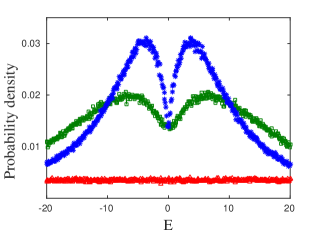
Figure 4: (Color online) TLS DOS for different disorder values. $W=1$ (blue stars), $W=10$ (green squares), and $W=100$ (red triangles) for $W/T=10$, constant interactions $J=1$ and $N=1000$. $r_{nn}=1$ as in all our calculations.

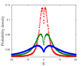
Figure 5: (Color online) TLS DOS for different interaction and disorder values. $W/J=1$ (blue asterisks), $W/J=3.1$ (green squares), and $W/J=9.8$ (red triangles), keeping $W^{2}+J^{2}=2$. $N=1000$ and $T=0.1$. The structure of the DOS including the gap and the peaks around it is getting narrower and higher for larger values of $W/J$.

The study of the DOS of the TLS-glass is of interest by itself, but also in view of our interest in the dynamics of the TLS-glass. As can be inferred from Eq. (12), the dynamics of the TLS-glass is strongly affected by the distribution of the single-TLS DOS. In fact, for a given realization of TLSs and constant temperature, there is a unique correspondence between the distribution of TLS energies and their dynamics. Thus, the change in DOS as function of varying disorder and interactions is a predictor of the change in the dynamics of the TLS-glass. In Fig. 4 and Fig. 5 we plot the single-TLS DOS as a function of varying disorder and interaction according to the protocols described above (see also figure caption). We find that for larger $W$ or $J$ the width of the DOS increases. Also, for larger ratio $J/W$ the depth of the gap increases as expected. Note that in the disorder variation scheme, large values of disorder are taken in order to obtain a large enough qualitative effect in the rates distribution (plotted in Sec. IV.2 below).

IV.2 Shift of the distribution of relaxation rates

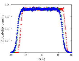
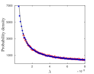
Figure 6: (Color online) TG decay rate distribution for different disorder values. $W=1$ (blue stars), $W=10$ (green squares), and $W=100$ (red triangles). $W/T=10$, $J=1$, and $N=1000$. (a) Rate distributions in log scale. (b) Rate distributions in normal scale. The values for $W=10$ are similar to those of $W=1$ and are therefore discarded.

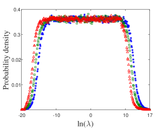
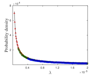
Figure 7: (Color online) TG decay rate distribution for different interaction and disorder values. $W/J=1$ (blue asterisks), $W/J=3.1$ (green squares), and $W/J=9.8$ (red squares). The rest of the parameters are the same as in Fig. 5. (a) Rate distributions in log scale. (b) Rate distributions in normal scale.

The distributions of relaxation rates [Eq. (12)] for both of the schemes presented in Sec. IV.1 are plotted in Fig. 6 for the variation of $W$ and in Fig. 7 for the variation of $W/J$. As can be seen, for increasing $W$ or $J/W$ the rates distributions are shifted to higher values on the same $1/\lambda$ curve. This is a consequence of the shift of the lower cutoff with the variation of parameters. In turn, the lower cutoff represents TLSs which also have, in addition to small tunneling amplitude $\Delta_{0}$, small excitation energy. The number of such TLSs diminishes with the deepening of the gap and the enhancement of the variance of the DOS, leading to faster dynamics. Note that the upper cutoff is held fixed in the normal scale plots. This is due to the fact that the rates distribution extends over many orders of magnitude which are not relevant to the relaxation of the system at long time scales, i.e., $t\sim\lambda_{min}^{-1}$.

V Comparison to the electron-glass model

In this section we consider the electron-glass (EG) model and compare its equilibrium and dynamical properties to the results of the TG model shown in Sec. IV. In Sec. V.1 we review the results of Amir et al. Amir et al. (2008). We present the EG Hamiltonian, its equilibrium mean-field energies and the logarithmic relaxation which results from the $\frac{1}{|\lambda|}$ distribution of rates. In Sec. V.2 we address the effects of the disorder and interactions on the relaxation to facilitate comparison between the TG and EG models, and add in this subsection a discussion of the effects of system size. In Sec. V.3 we present additional similarities and differences which originate from the basic structure of the EG and TG models.

V.1 The electron-glass: Model and dynamics

The electron-glass (EG) system is composed of $N$ localized electronic states with random energies and $M<N$ electrons interacting via the unscreened Coulomb interaction. The electron-phonon coupling induces inter-site electron transitions. Since the Hubbard energy is assumed to be much greater than the energy scale of the system, only single occupation at each site is allowed. The exchange interaction is assumed to be much smaller than the Coulomb interaction, resulting in spinless electrons. Accordingly, the Hamiltonian of the EG system is Burin et al. (2006); Amir et al. (2011); Pollak et al. (2012)

$$\mathcal{H}_{EG}=\sum^{N}_{i=1}\epsilon_{i}\left(n_{i}-K\right)+\sum^{N}_{i=1}\sum_{j>i}\frac{e^{2}}{r_{ij}}\left(n_{i}-K\right)\left(n_{j}-K\right)$$ (19)

where $\epsilon_{i}$ are the random site energies of the system in the absence of interactions, $\frac{e^{2}}{r_{ij}}$ is the Coulomb interaction between the electrons at sites $i$ and $j$, $K=\frac{M}{N}$ is the background charge and $n_{i},n_{j}\in[0,1]$ are site occupations. The sites are distributed uniformly in a square. In equilibrium, the site occupations obey the Fermi-Dirac statistics, $n^{0}_{i}=\left(e^{E_{i}/T}+1\right)^{-1}$, and accordingly the self-consistent equations are

$$E_{i}=\epsilon_{i}-\frac{1}{2}\sum_{j\neq i}\frac{e^{2}}{r_{ij}}\tanh\left(\frac{E_{j}}{2T}\right)\,,$$ (20)

where $E_{i}$ are the MF energy of site $i$ and Boltzmann constant is set to unity. The DOS obtained from the self-consistent Eq. (20) shows a gap around the chemical potential, known as the Coulomb-gap, first predicted by Efros and Shklovskii Efros and Shklovskii (1975). Starting from randomly distributed values in each realization, the MF energies are found by an iterative procedure introduced by Grunewald et al. Grunewald et al. (1982). The numerical solution in 2D gives a linear density of states for low energiesAmir et al. (2008) (see also Fig. 8). As can be seen finite temperature introduces a finite DOS at correspondingly low energies. Similarly to the DOS of the TG model, for large enough temperature the gap disappears completely Davies et al. (1984); Levin et al. (1987); Pikus and Efros (1994).

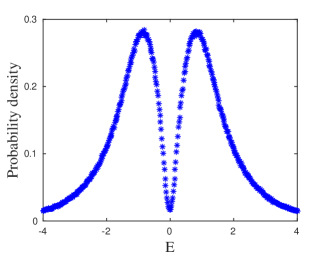
Figure 8: (Color online) EG DOS. The normalized histogram of site energies $E_{i}$ for half-filling and $N=10000$ sites Amir et al. (2008). The energies $\epsilon_{i}$ are uniformly distributed in the interval $[-\frac{W}{2},\frac{W}{2}]$, and $\frac{e^{2}}{r_{nn}T}=20$. $W=1$ and $E_{i}$ are taken in units of interaction at average nearest-neighbor distance $J=\frac{e^{2}}{r_{nn}}$, where $r_{nn}$ is the average nearest-neighbor distance. The sites are distributed uniformly on a square with periodic boundary condition and averaged over 300 realizations.

The dynamics of the average electronic occupations is calculated using the Pauli-rate equation (8) with Miller and Abrahams transition rates Miller and Abrahams (1960)

$$\gamma_{ij}=\Gamma^{0}_{ij}n_{i}\left(1-n_{j}\right)e^{-r_{ij}/\xi}\left[N(|\Delta E|)+\Theta(|\Delta E|)\right]\,.$$ (21)

Here $\Theta$ is a step function, $N=\left(e^{|\Delta E|/T}-1\right)^{-1}$ is the phonon occupation, $\Delta E=E_{i}-E_{j}$ and $\xi$ is the localization length of the electron. The prefactor is $\Gamma^{0}_{ij}\simeq\frac{2\pi}{\hbar}|M_{q}|^{2}\nu$, where $M_{q}$ is the strength of the electron-phonon interaction and $\nu$ is the phonon density of states. Since we are interested in a qualitative description of the dynamics, the rates will be presented in units of $\Gamma^{0}_{ij}$. The linearized rate equation for small deviation around equilibrium values is given by Amir et al. (2008)

$$\frac{d\delta n_{i}}{dt}=\sum_{j}A_{ij}\delta n_{j}\,$$ (22)

where the rate coefficients matrix take the form

$$A_{ij}=\begin{cases}\frac{\gamma^{0}_{ij}}{n^{0}_{j}\left(1-n^{0}_{j}\right)}-\sum_{k\neq j,i}\frac{e^{2}\gamma^{0}_{ik}}{T}\left(\frac{1}{r_{ij}}-\frac{1}{r_{jk}}\right)&;\;i\neq j\\ -\sum_{k}A_{kj}&;\;i=j\,.\end{cases}$$ (23)

The superscript $"0"$ indicates equilibrium values. The diagonal elements $A_{ii}$ are dictated by the requirement of particle number conservation, $\sum_{i}A_{ij}=0$. Neglecting the second term of the off-diagonal element of $A_{ij}$, the top line in Eq.(23) (the electron-electron interaction term has been shown to be insignificant at low temperatures Amir et al. (2008, 2009a)), one obtains the $\frac{1}{|\lambda|}$ distribution of relaxation rates Amir et al. (2008, 2010); see also Fig. 9. Notice that according to the definition of Eq. (23) the rates will turn out to be negative.

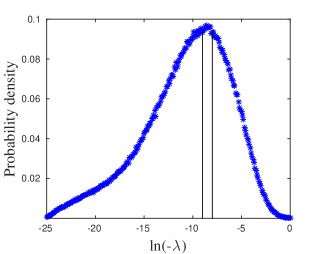
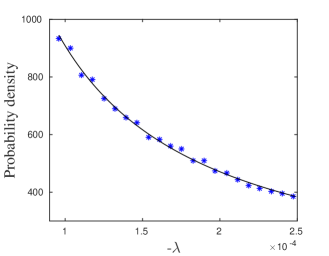
Figure 9: (Color online) Decay rate distribution for the electron-glass. Normalized histograms of the real part of the decay rates (originally done elsewhere Amir et al. (2008)), obtained by numerical diagonalization of the rate matrix $A_{ij}$ given in Eq. (23), while neglecting the direct interactions term. $N=1000$, $\frac{e^{2}}{r_{nn}T}=10$, and $\frac{r_{nn}}{\xi}=10$. The disorder energy and density of sites are the same as in Fig. 8. The graph is averaged over 1000 realizations. (a) Rate distribution in log scale. The cutoff values are taken around the plateau region. (b) Rate distribution in normal scale with a $\frac{1}{\lambda}$ fit. The region of the plot is determined by the cutoffs as seen in the log plot.

Solving the linearized rate equation and going through the steps shown in Sec. III, the obtained total relaxation of the EG systems for times $\frac{1}{\lambda_{max}}<t<\frac{1}{\lambda_{min}}$ and $p(\lambda)=\frac{1}{\lambda}$ rate distribution is (Amir et al., 2008):

$$|\bm{\delta n}|\simeq c\int_{\lambda_{min}}^{\lambda_{max}}\frac{e^{-\lambda t}}{\lambda}d\lambda\simeq-c[\gamma_{E}+log(\lambda_{min}t)]$$ (24)

where the assumption is that the rate matrix eigenvectors are excited roughly with a uniform probability $c(\lambda)\simeq c$ except for the eigenvector associated with the zero eigenvalue which can not be excited since the total particle number is conserved.

V.2 The effect of interactions and disorder in the EG model

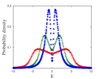
Figure 10: (Color online) EG DOS for different disorder values. $W=1$ (blue stars), $W=5$ (green squares) and $W=10$ (red triangles) for $W/T=10$, constant interactions $J=1$, and $N=1000$. The density of sites is set as in Fig. 8.

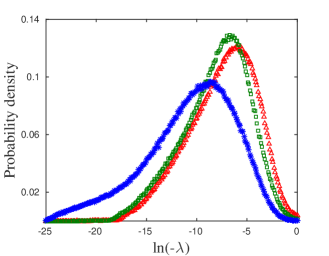
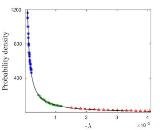
Figure 11: (Color online) EG decay rate distribution as given by the distribution of eigenvalues of the rate matrix in Eq. (22)Amir et al. (2008), for different disorder values. The parameters are the same as in Fig. 10. (a) Rate distributions in log scale. (b) Rate distributions in linear scale.

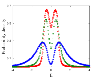
Figure 12: (Color online) EG DOS for different interaction and disorder values. $W/J=1$ (blue stars), $W/J=\sqrt{17}$ (green squares) and $W/J=\sqrt{97}$ (red triangles) for constant sum of variances $W^{2}+J^{2}=2$, temperature $T=0.1$, and $N=1000$. The density of sites is set as in Fig .8.

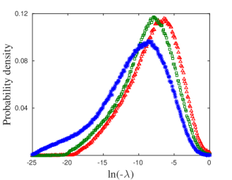
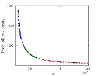
Figure 13: (Color online) EG decay rate distribution as given by the distribution of eigenvalues of the rate matrix in Eq. (22)Amir et al. (2008), for different values of the parameter $J/W$. The parameters are the same as in Fig. 12. (a) Rate distribution in log scale. (b) Rate distributions in linear scale.

To compare between the TG model and the EG model we perform the same parameter-varying schemes for the electron-glass model as presented in the previous section for the TG model (i.e., varying $W$ and $J/W$; see Sec. IV.1) and study how the DOS and rates are affected. This is done by studying the typical change of the rate matrix element, Eq. (23), without the electron-electron interaction term Amir et al. (2008, 2009a), and use it as a measure for the shift of the rates. Note that the plateau region in the rate log plots of the EG model is narrower than in the TG model allowing us conveniently to take also the upper cutoff. Figures 10 and 11 show respectively that for increasing disorder the DOS broadens while the gap diminishes (although the enhancement of the DOS near zero energy is a direct consequence of the variation of temperature in that scheme) leading to a shift of the rates to higher values, even though the disorder is stronger. Figures 12 and 13 show respectively how for increasing interactions the DOS broadens and the gap deepens, and at the same time a shift of the rates to lower values, opposite to the effect of interactions on the TG relaxation rates. Unlike the case for the TLS-glass, for the EG the connection between the single particle DOS and the relaxation rate distribution is indirect. The DOS affects the $N^{2}-N$ hopping rates $A_{ij}$, which constitute the matrix whose $N$ eigenvalues are the relaxation rates. Still, some intuition may be obtained by considering the dependence of $A_{ij}$ on the energy difference between the sites $i,j$ for low temperatures:

$$A_{ij}\sim N(\Delta E)\sim\begin{cases}1&,\Delta E>T,\;\Delta E<0\\ e^{-\Delta E/T}&,\Delta E>T,\;\Delta E>0\\ \frac{T}{|\Delta E|}&,|\Delta E|<T\end{cases}.$$ (25)

Narrower gaps and a larger DOS at low energies enhance the weight of small energy differences between near neighbor sites, which in turn leads to faster relaxation.

Finally, it is worth mentioning the results obtained for changing the system size. Both for the EG and TG models we found numerically that increasing the number of sites (while keeping a constant density) shifts the rate distribution to lower values. Specifically for the TG model, we found the shift to be negligible whereas for the EG the effect is more pronounced. It turns out that the shift in the EG model is a finite-size effect that originates from the statistics of the exponential distance matrix ($e^{-r_{ij}/\xi}$) rather than from the dependence on the interactions; see App. A. The fact that the interactions have a negligible contribution to the change in dynamics as the system size is enhanced, in both models, suggests that the relaxation modes are local in nature.

Table 1 summarizes the effects of disorder, interactions, and system size on the dynamics of the EG and TG models.

Model/Quantity	Disorder	Interaction	System size
EG	$+$	$-$	$-$
TG	$+$	$+$	$-$

Table 1: (Color online) Comparison between the relaxation dynamics of the EG and the TG models for increasing disorder $(W)$, interactions $(J)$, and system size $(N)$. The $(+)$ and $(-)$ signs indicate faster and slower relaxation respectively. Note that for changing the system size, the dynamics has a weak dependence on the mean-field energies (and thus on the interaction $J$) in both models, which implies that the relaxation modes are local.

V.3 Structural comparison of the EG and TG models

In this section we compare the formal solutions of the EG and TG models. First, comparing Eqs. (12), (28)and Eqs. (23), (22) we see that the interaction term of the EG rate equation includes also an interaction and transition with a third site whereas the second term in the TG rate equation does not. This difference stems from the fact that transitions are allowed only within pairs of states (TLSs act as dimers). The interactions are then between two dimers, whereas in the EG model the interactions are between single site occupations. This leads to the notion that under a certain condition one may obtain the mathematical structure of the TG model from the given EG model. This happens when the distance between next nearest-neighbor ($r_{nnn}$) is sufficiently larger than the nearest-neighbor distance ($r_{nn}$), i.e., $r_{nnn}-r_{nn}>2\xi$.

Also, in both models the $\frac{1}{|\lambda|}$ distribution of relaxation rates leading to logarithmic relaxation is a result of the wide and rather homogeneous distribution of an exponent, i.e., $A_{ij}\propto e^{-r_{ij}/\xi}$ in Eq. (23) in the EG model and $\Delta_{0}\propto e^{-\Lambda}$ in the TG model. However, the range in which the $\frac{1}{|\lambda|}$ form is satisfied is much wider in the TG model (Fig. 3) than in the EG’s (Fig. 9). This is a result of the exponent in the TLS glass model being chosen as homogeneous over a large regime, whereas in the EG model the tunneling amplitude is dictated by the distribution of nearest-neighbor distances, which is narrower. Last, the different dependence of the rates on the mean-field energies in the two models leads to the different consequences of varying the interactions, disorder, and system size on the dynamics of the two models.

VI Summary and conclusions

In this work we examine thermodynamic and dynamic properties of the TLS-glass, modeled by the transverse field Ising model with random $1/r^{3}$ interactions and random local fields. Using mean field approximation, we first rederive the single particle DOS for this model, and then derive the dynamics of its relaxation to equilibrium. Similarly to the electron glass model, we find $1/\lambda$ distribution of relaxation rates, leading to logarithmic time relaxation and known memory effects in such models Vaknin et al. (2000); Amir et al. (2009b). We further find that increasing the disorder shifts the rate distribution to higher values, similarly to what was observed for the electron glassAmir et al. (2008), but increasing the interactions shifts the rate distribution to higher values while in the EG model this results in a shift to lower valuesAmir et al. (2008). This suggests that the effect of interactions on glass dynamics is system dependent. Finally, we show that the interactions have a negligible effect on the rate distribution for changing the system size at constant site density, which implies that the relaxation modes are localized.

Given the complexity of the EG and TG models we use the MF approximation which simplifies the calculation. It would be of interest to check our results for the dynamics of the system, some of them unexpected, against more exact numerical methods such as Monte Carlo simulations or exact diagonalization of finite systems.

Appendix A Finite-size effect in the EG model

In this appendix we give a qualitative argument that explains the shift of the rate distribution caused by changing the system size in the EG model.

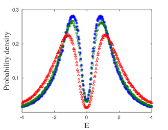
Figure 14: (Color online) EG DOS for different system sizes. The number of sites $N$ is varied, $10$ (red triangles), $100$ (green squares), $1000$ (blue asterisks). $\frac{e^{2}}{r_{nn}T}=10$. The disorder and density of sites are the same as in Fig. 8. Notice how the DOS is wider and the gap is shorter for smaller number of sites. The same quantitative behavior can be seen for changing the interactions strength to smaller values.

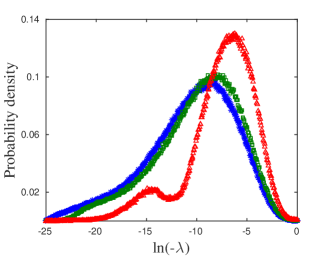
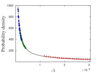
Figure 15: (Color online) EG decay rate distribution as given by the distribution of eigenvalues of the rate matrix in Eq. (22), for different system sizes. $N=10$ (red triangles), $N=100$ (green squares), and $N=1000$ (blue asterisks). Localization length $\xi=0.1$. Disorder energy $W$ and density of sites are the same as in Fig. 8. The solid line is a fit of $1/x$ curve. (a) Rate distributions in the natural log scale. (b) Rate distributions in linear scale.

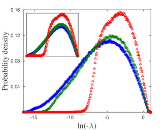
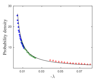
Figure 16: (Color online) EG rate distribution as given by the eigenvalue distribution of the matrix $A_{ij}=e^{-r_{ij}/\xi}$ (without energy dependence), plotted for different system sizes. $N=1000$ (blue stars), $N=100$ (green squares), and $N=10$ (red triangles). The parameters are the same as in Fig. 15. (a) Rate distributions in the natural log scale. The inset shows how the peaks almost coincide after scaling $\xi$ with the prefactor given in Eq. (27). (b) Rate distributions in linear scale.

In Fig. 14 the EG DOS is plotted for different system sizes, showing a narrowing of the gap for increasing size. In Fig. 15 the EG relaxation rate distribution is plotted showing a shift to lower values for increasing system size, which might seem counter intuitive given the behavior of the DOS. We show below how this shift is dominated by the tunneling term.

Figure 16 shows the rate distribution as given in Fig. 15 after excluding the interactions term in the rate matrix, i.e., $A_{ij}=e^{-r_{ij}/\xi}$. Comparing the two graphs it is evident that the shift of the rate distribution peaks remains qualitatively the same.

Let us now estimate this effect. For $r_{nn}\ll\xi$, the relaxation is dominated by tunneling of electrons to their near neighbor site. Given a linear size of the sample $L$ it can be shown that the distribution of nearest-neighbor distance for $r_{nn}\ll L$ isAmir et al. (2008)

$$p(r)=\frac{V_{d}}{L^{d}}d(N-1)r^{d-1}e^{-V_{d}(N-1)(r/L)^{d}}\,,$$ (26)

where $r$ is the nearest-neighbor distance in the continuous limit, $d$ is the dimension, and $V_{d}$ is of order unity, e.g. $V_{1}=2$, $V_{2}=\pi$. Substituting the average nearest-neighbor distance $\bar{r}=L^{d}/(N^{1/d}-1)$ for constant site density, as used in the numerical calculation, and changing to variable $x=\log(-\frac{\lambda}{2})=-\frac{r}{\xi}$Amir et al. (2008) we obtain for $d=2$:

$$p(x)=2\pi\left(\frac{\xi}{\bar{r}}\right)^{2}x\frac{\sqrt{N}+1}{\sqrt{N}-1}\exp{\left[-\pi\left(\frac{\xi}{\bar{r}}\right)^{2}x^{2}\frac{\sqrt{N}+1}{\sqrt{N}-1}\right]}\,.$$ (27)

As can be seen from Eq. 27, $p(x)$ shifts with system size ($N$) in the same qualitative manner as obtained numerically in Fig. 16. Furthermore, the inset shows the distributions when scaled according to Eq. 27 $x\rightarrow x\left(\frac{\sqrt{N}+1}{\sqrt{N}-1}\right)^{\frac{1}{2}}$. This suggests that within the mean-field approximation discussed in this work, the dominant cause for the slow down of relaxation is a finite-size effect that changes the effective average near neighbor distance. In similarity to the EG, the TG also shows slowing down of the relaxation with increased system size, but the effect is much weaker (not shown). Note though that for the TG model the relaxation rates are dictated by the tunneling amplitudes $\Delta_{0i}$, which are distributed independently from the site distribution of the TLSs and therefore the relaxation rate distribution is not sensitive to finite-size effects.

Appendix B Interaction term in the rate equation

In this appendix we discuss the full linearized rate equation (Eq. 13 with the addition of interaction terms)

$$\frac{d\sigma_{i}}{dt}\simeq-\lambda_{i}\delta\sigma_{i}+\sum_{j\neq i}f_{ij}\delta\sigma_{j}\equiv\sum_{j}A_{ij}\delta\sigma_{j}$$ (28)

and show that the second term can be neglected at low temperatures. Here $f_{ij}=2a_{i}\Delta^{2}_{0i}\Delta^{\prime}_{i}N_{i}(N_{i}+1)\sigma^{0}_{i}\frac{u_{ij}}{Tr^{3}_{ij}}$ is the interaction prefactor and $n_{i}=\left(e^{\beta|E_{i}|}-1\right)^{-1}$, $\sigma^{0}_{i}=-\tanh\left(\frac{E_{i}}{2T}\right)$ are the phonon and pseudospin equilibrium occupations.

An estimate for the contribution of interaction term to the rate equation is given by the ratio

$$\left|f_{ij}/\lambda_{i}\right|=\left|\frac{\Delta^{\prime}_{i}}{|E_{i}|\cosh^{2}\left(\frac{E_{i}}{2T}\right)}\frac{u_{ij}}{Tr_{ij}^{3}}\right|\lesssim\left|\frac{\Delta^{\prime}_{i}}{|E_{i}|\cosh^{2}\left(\frac{E_{i}}{2T}\right)}\frac{J}{T}\right|\,.$$ (29)

The second inequality represents an upper bound, where $i,j$ are nearest-neighbor, i.e. $\frac{u_{ij}}{r^{3}_{ij}}=\frac{U_{0}}{r^{3}_{nn}}\equiv J$. Furthermore, since both $\lambda_{i}$ and $f_{ij}$ are proportional to $\Delta^{2}_{0i}$, the lowest rates (eigenvalues of $A_{ij}$), which dictate the slow relaxation of the system, have a tunneling amplitudes $\Delta_{0i}\sim\Delta_{0_{min}}$. Thus, one can approximate $\Delta^{\prime}_{i}\approx E_{i}$ and substitute in Eq. 29:

$$\begin{split}&\max(|f_{ij}/\lambda_{i}|)=\\ &=\begin{cases}\frac{J}{T}\left[1+\frac{1}{2}\left(\frac{E_{i}}{2T}\right)^{2}\right]^{-1}\longrightarrow\frac{J}{T}&,|E_{i}|\ll T\\ 0.1\frac{J}{T}<|f_{ij}/\lambda_{i}|<\frac{J}{T}&,|E_{i}|<2T\\ 2\frac{J}{T}e^{-|E_{i}|/T}&,|E_{i}|>2T\end{cases}\end{split}$$ (30)

As can be seem from Eq. 30, at low temperatures relative to disorder and interactions ($T\ll\sqrt{W^{2}+J^{2}}$) the typical TLS energy is larger then the temperature and $f_{ij}$ is exponentially suppressed.

Let us further consider two different limit cases: (i) $T\sim W\ll J$. In this case TLSs with $f_{ij}\sim\lambda_{i}$ are rare since the temperature resides deep inside the dipole gap. (ii) $T\sim J\ll W$. In this case the gap is small but the DOS is flat and wide in comparison to the temperature scale, and the number of TLSs with energy smaller then the temperature is $N(|E_{i}|<2T)\propto\frac{T}{W}\ll 1$.

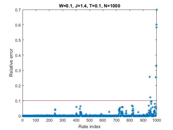
Figure 17: Relative error between the rates with and without the interaction term $f_{ij}$, for W=0.1, J=1.4, T=0.1, and N=1000.

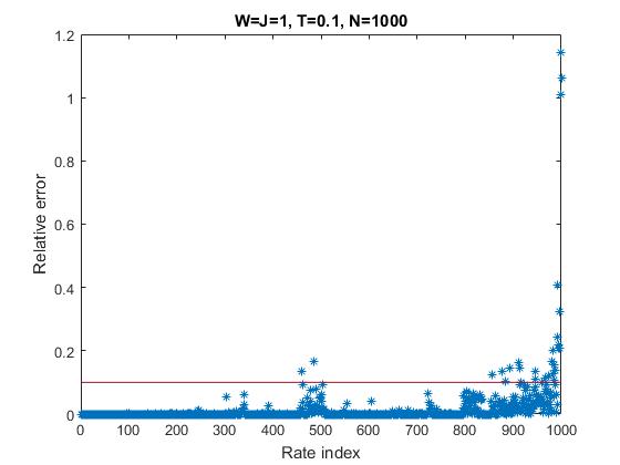
Figure 18: Relative error between the rates with and without the interaction term $f_{ij}$, W=J=1, T=0.1, and N=1000.

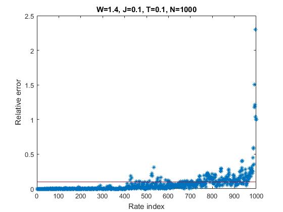
Figure 19: Relative error between the rates with and without the interaction term $f_{ij}$, W=1.4, J=0.1, T=0.1, and N=1000.

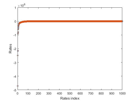
Figure 20: Typical graph of the rates with and without the interaction term for the three cases stated above. Blue (asterisk) for $f_{ij}=0$ and orange (plus) is for $f_{ij}\neq 0$.

To substantiate the conclusion that the interaction term in the rate equation has little effect on the dynamics of the system at low temperatures, we diagonalize numerically the rate matrix $A_{ij}$ in Eq. (28) and compare with the results obtained neglecting the interaction term. The graphs presented below show the relative error, defined as $\left|\frac{\lambda^{\prime}-\lambda}{\lambda^{\prime}}\right|$, where $\lambda^{\prime}$ ($\lambda$) are the rates including (excluding) interactions, for three cases: (i) $W\simeq 1.4,J\simeq 0.1$ (Fig 17), (ii) $W\simeq 0.1,J\simeq 1.4$ (Fig 18), (iii) $W=J=1$ (Fig 19). For all cases we numerically diagonalise a single realization of $A_{ij}$ for $N=1000$, $W^{2}+J^{2}=2$ and $T=0.1$. In all cases low rates are negligibly affected by the interaction. In Fig 20 we present the rates for $W=J=1$ [case (i)] with and without interactions. Similar results were obtained for cases (ii) and (iii).

References

- Zeller and Pohl (1971) R. C. Zeller and R. O. Pohl, Phys. Rev. B 4, 2029 (1971).
- Anderson et al. (1972) P. W. Anderson, B. I. Halperin, and C. M. Varma, Philosophical Magazine 25, 1 (1972).
- Phillips (1972) W. Phillips, Journal of Low Temperature Physics 7, 351 (1972).
- Phillips (1987) W. A. Phillips, Reports on Progress in Physics 50, 1657 (1987).
- Black and Halperin (1977) J. L. Black and B. I. Halperin, Phys. Rev. B 16, 2879 (1977).
- Burin and Kagan (1994) A. Burin and Y. Kagan, Journal of Experimental and Theoretical Physics (1994).
- Rogge et al. (1996) S. Rogge, D. Natelson, and D. D. Osheroff, Phys. Rev. Lett. 76, 3136 (1996).
- Natelson et al. (1998) D. Natelson, D. Rosenberg, and D. D. Osheroff, Phys. Rev. Lett. 80, 4689 (1998).
- Neeley et al. (2008) M. Neeley, M. Ansmann, R. C. Bialczak, M. Hofheinz, N. Katz, E. Lucero, A. O/’Connell, H. Wang, A. N. Cleland, and J. M. Martinis, Nat Phys 4, 523 (2008).
- Simmonds et al. (2004) R. W. Simmonds, K. M. Lang, D. A. Hite, S. Nam, D. P. Pappas, and J. M. Martinis, Phys. Rev. Lett. 93, 077003 (2004).
- Barends et al. (2014) R. Barends, J. Kelly, A. Megrant, A. Veitia, D. Sank, E. Jeffrey, T. C. White, J. Mutus, A. G. Fowler, B. Campbell, Y. Chen, Z. Chen, B. Chiaro, A. Dunsworth, C. Neill, P. O/’Malley, P. Roushan, A. Vainsencher, J. Wenner, A. N. Korotkov, A. N. Cleland, and J. M. Martinis, Nature 508, 500 (2014), letter.
- Shalibo et al. (2010) Y. Shalibo, Y. Rofe, D. Shwa, F. Zeides, M. Neeley, J. M. Martinis, and N. Katz, Phys. Rev. Lett. 105, 177001 (2010).
- Lisenfeld et al. (2016) J. Lisenfeld, A. Bilmes, S. Matityahu, S. Zanker, M. Marthaler, M. Schechter, G. Schön, A. Shnirman, G. Weiss, and A. V. Ustinov, Scientific reports 6 (2016).
- Matityahu et al. (2016) S. Matityahu, A. Shnirman, G. Schön, and M. Schechter, Phys. Rev. B 93, 134208 (2016).
- Lisenfeld et al. (2015) J. Lisenfeld, G. J. Grabovskij, C. Müller, J. H. Cole, G. Weiss, and A. V. Ustinov, Nat Commun 6 (2015).
- Lisenfeld et al. (2010) J. Lisenfeld, C. Müller, J. H. Cole, P. Bushev, A. Lukashenko, A. Shnirman, and A. V. Ustinov, Phys. Rev. Lett. 105, 230504 (2010).
- Grabovskij et al. (2012) G. J. Grabovskij, T. Peichl, J. Lisenfeld, G. Weiss, and A. V. Ustinov, Science 338, 232 (2012).
- Müller et al. (2015) C. Müller, J. Lisenfeld, A. Shnirman, and S. Poletto, Phys. Rev. B 92, 035442 (2015).
- Burin (1995) A. Burin, Journal of Low Temperature Physics 100, 309 (1995).
- Burin et al. (1998) A. L. Burin, D. Natelson, D. D. Osheroff, and Y. Kagan, in Tunneling Systems in Amorphous and Crystalline Solids (Springer, 1998) pp. 223–315.
- Burin and Kagan (1996) A. Burin and Y. Kagan, Physics Letters A 215, 191 (1996).
- Amir et al. (2008) A. Amir, Y. Oreg, and Y. Imry, Phys. Rev. B 77, 165207 (2008).
- Churkin et al. (2014) A. Churkin, D. Barash, and M. Schechter, Phys. Rev. B 89, 104202 (2014).
- Schechter and Stamp (2013) M. Schechter and P. C. E. Stamp, Phys. Rev. B 88, 174202 (2013).
- Churkin et al. (2013) A. Churkin, I. Gabdank, A. Burin, and M. Schechter, arXiv preprint arXiv:1307.0868 (2013).
- Baranovskii et al. (1980) S. Baranovskii, B. Shklovskii, and A. Efros, Soviet Journal of Experimental and Theoretical Physics 51, 199 (1980).
- Cuevas et al. (1989) E. Cuevas, R. Chicón, and M. Ortuño, Physica B: Condensed Matter 160, 293 (1989).
- Efros and Shklovskii (1975) A. L. Efros and B. I. Shklovskii, Journal of Physics C: Solid State Physics 8, L49 (1975).
- Grunewald et al. (1982) M. Grunewald, B. Pohlmann, L. Schweitzer, and D. Wurtz, Journal of Physics C: Solid State Physics 15, L1153 (1982).
- Jäckle (1972) J. Jäckle, Zeitschrift für Physik 257, 212 (1972).
- Bender and Orszag (1999) C. M. Bender and S. A. Orszag, Advanced Mathematical Methods for Scientists and Engineers: Asymptotic methods and perturbation theory (Springer, 1999) p. 252.
- Amir et al. (2012) A. Amir, Y. Oreg, and Y. Imry, Proceedings of the National Academy of Sciences 109, 1850 (2012).
- Burin et al. (2006) A. L. Burin, B. I. Shklovskii, V. I. Kozub, Y. M. Galperin, and V. Vinokur, Phys. Rev. B 74, 075205 (2006).
- Amir et al. (2011) A. Amir, Y. Oreg, and Y. Imry, Annual Review of Condensed Matter Physics 2, 235 (2011).
- Pollak et al. (2012) M. Pollak, M. Ortuño, and A. Frydman, The Electron Glass: (Cambridge University Press, Cambridge, 2012).
- Davies et al. (1984) J. H. Davies, P. A. Lee, and T. M. Rice, Phys. Rev. B 29, 4260 (1984).
- Levin et al. (1987) E. Levin, V. Nguen, B. Shklovsii, and A. Efros, Soviet Physics JETP 65, 842 (1987).
- Pikus and Efros (1994) F. G. Pikus and A. L. Efros, Phys. Rev. Lett. 73, 3014 (1994).
- Miller and Abrahams (1960) A. Miller and E. Abrahams, Phys. Rev. 120, 745 (1960).
- Amir et al. (2009a) A. Amir, Y. Oreg, and Y. Imry, Phys. Rev. B 80, 245214 (2009a).
- Amir et al. (2010) A. Amir, Y. Oreg, and Y. Imry, Phys. Rev. Lett. 105, 070601 (2010).
- Vaknin et al. (2000) A. Vaknin, Z. Ovadyahu, and M. Pollak, Phys. Rev. Lett. 84, 3402 (2000).
- Amir et al. (2009b) A. Amir, Y. Oreg, and Y. Imry, Phys. Rev. Lett. 103, 126403 (2009b).