Drag coefficient of a liquid domain in a fluid membrane
with the membrane viscosities being different
across the domain perimeter

Abstract

We calculate the drag coefficient of a liquid domain in a flat fluid membrane surrounded by three-dimensional fluids on both sides. In the membrane, the tangential stress should be continuous across the domain perimeter, which makes the velocity gradient discontinuous there unless the ratio of the membrane viscosity inside the domain to the one outside the domain equals unity. The gradient of the velocity field in the three-dimensional fluids is continuous. This field, in the limit that the spatial point approaches the membrane, should agree with the velocity field of the membrane. Thus, unless the ratio of the membrane viscosities is unity, we need to assume some additional singularity at the domain perimeter in solving the governing equations. In our result, the drag coefficient is given in a series expansion with respect to a dimensionless parameter, which equals zero when the ratio of the membrane viscosities is unity and approaches unity when the ratio tends to infinity. We derive the recurrence equations for the coefficients of the series. In the limit of the infinite ratio, our numerical results agree with the previous results for the disk.

1 Introduction

The magnitude of the drag force exerted on a colloidal particle moving slowly enough in a fluid is proportional to its speed. The constant of the proportion is called drag coefficient, of which reciprocal gives the diffusion coefficient after being multiplied by the Boltzmann constant and temperature (Sutherland, 1905; Einstein, 1905). Calculating the drag coefficient is one of the fundamental problems in the low-Reynolds number hydrodynamics (Happel and Brenner, 1983). Most well-known is the drag coefficient of a rigid sphere in a three dimensional (3D) fluid (Stokes, 1851). That of a droplet is also well known (Hadamard, 1911; Rybczynski, 1911). The latter tends to the former as the ratio of the viscosity of the droplet to that of the ambient fluid approaches infinity. It is to be noted that we need not consider droplet deformation in this linear regime.

One can neglect the inertia term to use the Stokes equation when the Reynolds number is small. The drag coefficient of a disk in a two-dimensional (2D) fluid cannot be calculated in the Stokes approximation (Lamb, 1932). This Stokes paradox can be helped when the fluid is sandwiched by 3D fluids. This situation, for example, is realized by using a lipid-bilayer membrane, which is the main part of biomembrane and has the fluidity (Singer and Nicolson, 1972). The drag coefficient was calculated for a small disk in a flat fluid membrane surrounded by 3D fluids occupying semi-infinite spaces on both sides (Saffman and Delbrück, 1975; Saffman, 1976); the result was utilized experimentally (Peters and Cherry (1982)). Theoretically, in this geometry, we use the cylindrical coordinates to introduce the Hankel transformation. In the end, we need to solve a set of integral equations, which were studied extensively (Sneddon, 1966; Hughes et al., 1981).

The main lipid component of the biomembrane is phospholipid. Some minor lipid components are concentrated to form a liquid domain called a lipid raft, which is ten to several hundreds nanometer in size (Parton and Simons, 1995; Simons and Toomre, 2000; Subczynski and Kusumi, 2003). It is thought to play significant roles in biological activities, for instance, in the signal transduction. Raft-like liquid domains in an artificial fluid membrane have also been studied in the context of phase separation (Veatch and Keller, 2005; Yanagisawa et al., 2007). The drag coefficient of a liquid domain whose membrane viscosity $(\eta_{\rm i})$ equals the one outside the domain $(\eta_{\rm o})$ was calculated in Koker (1996). Here, we introduce a dimensionless parameter defined as

$$\kappa\equiv 1-{\eta_{\rm o}\over\eta_{\rm i}}\ .$$ (1.1)

In Koker (1996), $\kappa$ is supposed to vanish. Cases where the membrane viscosities are slightly different were studied in Fujitani (2011), where the drag coefficient is calculated up to a linear order of $\kappa$. However, as described later, one boundary condition is overlooked there. This error is corrected and the drag coefficient is recalculated up to the same order in Fujitani (2013). In the present study, using the corrected boundary condition, we calculate the drag coefficient of a liquid domain by considering terms of higher order with respect to $\kappa$. In particular, as $\kappa$ approaches unity, i.e., as $\eta_{\rm o}$ becomes much larger than $\eta_{\rm i}$, our result successfully tends to the drag coefficient of a disk, which is calculated by the formula obtained in Hughes et al. (1981). A related work is found in Rao and Das (2015), where the uncorrected boundary condition of Fujitani (2011) were somehow used although Fujitani (2013) was cited.

Our calculation involves the numerical integration, for which we use the software of Wolfram Mathematica^® ver. 10 (Wolfram Research). Our formulation is stated in Sect. 2. We show the previous results in Sect. 3. Our results are shown in Sect. 4, and some details of the procedure are relegated to Appendices. The formulation and most part of the procedure are the same as given in Fujitani (2013); we here show their key points indispensable for this paper to be self-contained. The last section is devoted to discussion.

2 Formulation

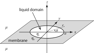
Figure 1: A raft-like liquid domain with radius $a$ and viscosity $\eta_{\rm i}$ is embedded in a fluid membrane stretching on the $xy$-plane infinitely. The membrane viscosity outside the domain is denoted by $\eta_{\rm o}$. The semi-infinite spaces on both sides of the membrane are fulfilled by 3D fluids sharing the same viscosity $\mu$.

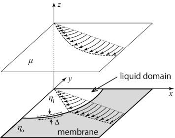
Figure 2: A region of $x>0$, $y<0$ and $z\geq 0$ of fig. 2 is drawn. The curved arrows represent velocity fields. In the membrane, the velocity gradient should be discontinuous across the domain perimeter when $\eta_{\rm i}$ is not equal to $\eta_{\rm o}$. In the 3D fluid, the velocity gradient is continuous, as shown in a cross section parallel to the membrane. A slender region is drawn with the dotted closed curve along the domain perimeter in the membrane. We write $\Delta$ for the size in the direction vertical to the perimeter.

As is shown schematically in fig. 2, the membrane is assumed to lie on the $xy$-plane of the Cartesian coordinate system $(x,y,z)$. We also set the cylindrical coordinates $(r,\theta,z)$ so that the line $\theta=0$ is the $x$-axis. A circular liquid domain with the radius $a$ shifts translationally with the velocity $\mbox{\boldmath$U$}=U\mbox{\boldmath$e$}_{x}$, where $\mbox{\boldmath$e$}_{x}$ denotes the unit vector of the $x$-axis. We consider the instant when the center coincides with the origin. The 3D fluids on both sides of the membrane share the same viscosity $\mu$. The drag force can be written as ${\cal F}_{x}\,{\mbox{\boldmath$e$}}_{x}$, and the drag coefficient $\gamma$ is given by $-{\cal F}_{x}/U$.

The velocity field in the 3D fluids and that of the fluid membrane are respectively denoted by $V$ and $v$. In this setting, we have

$$\lim_{r\to a}v_{r}(r,\theta)=U_{r}\ ,$$ (2.1)

where $v_{r}$ and $U_{r}$ denote the $r$-components of $v$ and $U$, respectively. Because of the no-slip condition, we also have

$$\lim_{z\to 0}{\mbox{\boldmath$V$}}(r,\theta,z)={\mbox{\boldmath$v$}}(r,\theta)\ .$$ (2.2)

Suppose a 2D region along the domain perimeter, as shown in fig. 2; we write $\Delta$ for its width in the direction vertical to the perimeter. As the perimeter becomes thin, or $\Delta$ approaches zero, the forces exerted on the region should become balanced and the stress exerted by the ambient 3D fluids becomes negligible. Thus, the tangential stress of the 2D fluid should be continuous across the perimeter, which is represented by

$$\lim_{r\to a+}{\tau}_{r\theta}(r,\theta)=\lim_{r\to a-}{\tau}_{r\theta}(r,\theta)\ .$$ (2.3)

Here, $\tau$ denotes the stress tensor associated with $v$, and the limit $r\to a\pm$ indicates that $r$ approaches $a$ with $r-a$ being kept positive (negative). When $\eta_{\rm i}$ equals $\eta_{\rm o}$, we can do without eq. (2.3) because eq. (2.3) is automatically satisfied when eq. (2.2) holds and $V$ is smooth. However, when $\eta_{\rm i}$ is not equal to $\eta_{\rm o}$, eq. (2.3) makes the velocity gradient of the 2D fluid discontinuous across the perimeter, as shown in fig. 2. Then, we should require both eqs. (2.2) and (2.3). This point is overlooked in Fujitani (2011), as discussed later.

The 3D velocity field satisfies the Stokes equation and the incompressibility condition,

$$\mu\Delta{\mbox{\boldmath$V$}}=\nabla P\quad{\rm and}\quad\nabla\cdot{\mbox{\boldmath$V$}}=0\ ,$$ (2.4)

where $P$ denotes the pressure field. Equation (2.4) holds for $z\neq 0$. The 2D velocity field of the membrane fluid also satisfies the Stokes equation and the incompressibility condition,

$$\eta\Delta{\mbox{\boldmath$v$}}+{\mbox{\boldmath$F$}}=\nabla p\quad{\rm and}\quad\nabla\cdot{\mbox{\boldmath$v$}}=0\ ,$$ (2.5)

where $p$ denotes the in-plane pressure field of the 2D fluid and $F$ denotes the stress exerted by the 3D fluids. The differential operators are defined in terms of $x$ and $y$ in eq. (2.5), which holds for $z=0$ and $r\neq a$. The membrane viscosity $\eta$ equals $\eta_{\rm i}$ inside the domain $(r<a)$ and equals $\eta_{\rm o}$ outside the domain $(r>a)$.

3 Previous results

We introduce the Fourier transforms with respect to $\theta$, e.g.,

$$\tilde{V}_{zm}(r,z)=\frac{1}{2\pi}\int^{2\pi}_{0}\mbox{\rm d}\theta\,\,V_{z}(r,\theta,z)\mbox{\rm e}^{-\mbox{\scriptsize\rm i}m\theta}$$ (3.1)

with $m=0,\pm 1,\pm 2,\dots$, and the Hankel transforms with respect to $r$, e.g.,

$$\hat{V}_{zm}(\zeta,z)=\int^{\infty}_{0}\mbox{\rm d}r\,\,rJ_{m}(\zeta r)\tilde{V}_{zm}(r,z)\ ,$$ (3.2)

where $J_{m}$ is the Bessel function of the first kind. Because of the symmetry, only the fields with $m=\pm 1$ do not vanish. In each field, the transforms of $m=\pm 1$ are related with each other. Thus, we have only to consider the fields with $m=1$. As shown in Appendix A, we rewrite eq. (2.4) into the Hankel transforms and solve the resultant equations for $m=1$ with two functions of $\zeta$ being left undetermined. We can relate the two functions with the aid of the second equation of eq. (2.5), and thus have only to consider one undetermined function of $\zeta$. We use

$$R\equiv{r\over a}\quad{\rm and}\quad\nu_{\rm o}\equiv{\eta_{\rm o}\over 2\mu a}\ .$$ (3.3)

Utilizing that the left-hand side (lhs) of eq. (2.5) is irrotational, and calculating $F$ in terms of $V$, we obtain

$$0 = \int^{\infty}_{0}\mbox{\rm d}\zeta\,\,\zeta^{2}J_{1}(\zeta R)A(\zeta)\qquad{\rm for}\,\,1<R,\quad{\rm and}$$ (3.4)

$$0 = \int^{\infty}_{0}\mbox{\rm d}\zeta\,\,\zeta^{2}J_{1}(\zeta R)A(\zeta)\left(1-\frac{\kappa}{1+\nu_{\rm o}\,\zeta}\right)\qquad{\rm for}\,\,0\leq R<1\ ,$$ (3.5)

where $A$ is the undetermined function. In Fujitani (2013), the 3D fluid on each side of the membrane is assumed to be confined by the membrane and a wall, which is parallel to the membrane and lies at the distance $H$ from the membrane. Taking the limit of $H\to\infty$ in eqs. (3.1) and (3.2) in Fujitani (2013) gives eqs. (3.4) and (3.5) above. Equation (2.1) yields

$$2\mu a^{2}U=\int_{0}^{\infty}\mbox{\rm d}\zeta{J_{1}(\zeta)A(\zeta)\over\zeta\left(1+\nu_{\rm o}\zeta\right)},$$ (3.6)

which corresponds with eq. (2.37) of Fujitani (2013) because of eqs. (2.26), (3.8), and (3.13) there.

Let us define $q(R)$ as the integral of eq. (3.4) for $R\geq 0$. As shown in Fujitani (2013), we can arrive at the solution by assuming

$$q(R)=q_{1}(R)+c_{1}\delta\left(R-1\right)+c_{2}{{\rm d}\over{\rm d}R}\delta\left(R-1\right)\ ,$$ (3.7)

where $q_{1}(R)$ is a finite function vanishing for $R>1$, and $c_{1}$ and $c_{2}$ are constants independent of $R$. The third term on the right-hand side (rhs) above is missed in Fujitani (2011). Without this term, we can satisfy all the conditions other than eq. (2.3), but the resultant solution is naturally incorrect unless $\eta_{\rm i}$ equals $\eta_{\rm o}$. The third term is taken into account in Fujitani (2013). The second term gives a point source, while the third term gives a dipole source, which is analogous to the single-layer and double-layer potentials in the boundary integral, respectively (Pozrikidis, 1992). The Hankel transformation of eq. (3.7) involves the integral $Rq_{1}(R)J_{1}(\zeta R)$ over $0<R<1$. Rewriting this integral with the aid of eq. (3.5), we obtain

$$\zeta A(\zeta)=c_{1}J_{1}(\zeta)-c_{2}\zeta J_{0}(\zeta)+\kappa\int_{0}^{\infty}\mbox{\rm d}\xi\ {\xi^{2}A(\xi)\over 1+\nu_{\rm o}\xi}\int_{0}^{1}\mbox{\rm d}R\ RJ_{1}(\zeta R)J_{1}(\xi R)$$ (3.8)

$$\qquad=c_{1}J_{1}(\zeta)-c_{2}\zeta J_{0}(\zeta)+\kappa\,\zeta\int_{0}^{\infty}\mbox{\rm d}\xi\ K(\zeta,\xi)A(\xi)\ ,$$ (3.9)

where the kernel is defined as

$$K(\zeta,\xi)\equiv\frac{\xi^{2}}{\left(1+\nu_{\rm o}\xi\right)\zeta}\times\frac{\xi J_{0}(\xi)J_{1}(\zeta)-\zeta J_{0}(\zeta)J_{1}(\xi)}{\zeta^{2}-{\xi}^{2}}\ .$$ (3.10)

Equation (3.8) is essentially derived in Sect. 3.2 of Fujitani (2013) although not shown explicitly because the discussion is mainly focused on the order of $\kappa$ there. The constants $c_{1}$ and $c_{2}$ can be determined with the aid of eqs. (2.3) and (3.6). Another kernel, $M$, is used in Fujitani (2013); its definition and relation to $K$ are given by

$$M(\zeta,\xi) \equiv \frac{\xi}{1+\nu_{\rm o}\xi}\times\frac{\zeta J_{0}(\xi)J_{1}(\zeta)-\xi J_{0}(\zeta)J_{1}(\xi)}{\zeta^{2}-{\xi}^{2}}$$ (3.11)

$$= K(\zeta,\xi)+{\xi J_{0}(\xi)J_{1}(\zeta)\over\left(1+\nu_{\rm o}\xi\right)\zeta}\ .$$ (3.12)

Calculating the total force exerted on the liquid domain, as shown in Fujitani (2013), we find the drag coefficient to be given by

$$\gamma={\pi\over aU}\lim_{R\to 1+}\lim_{Z\to 0+}\int_{0}^{\infty}\mbox{\rm d}\zeta\ \zeta J_{2}(\zeta R)A(\zeta)\mbox{\rm e}^{-\zeta Z}\ ,$$ (3.13)

where we use $Z\equiv z/a$. This equation is easily derived from eqs. (2.24), (2.41) and (3.13) of Fujitani (2013).

When $\kappa$ vanishes, we have $c_{2}=0$ and find

$$A(\zeta)={2\mu a^{2}U\over Y_{0}(\nu_{\rm o})}{J_{1}(\zeta)\over\zeta}\quad{\rm for}\ \kappa=0\ ,$$ (3.14)

which is substituted into eq. (3.13) to yield the previous result of Koker (1996). Writing $\gamma_{\kappa=0}$ for his result of the drag coefficient, we have

$$\gamma_{\kappa=0}={2\pi\mu a\over Y_{0}(\nu_{\rm o})}\ ,$$ (3.15)

where $Y_{0}$ is defined as

$$Y_{0}(\nu_{\rm o})=\int_{0}^{\infty}\mbox{\rm d}\zeta\ \frac{J_{1}^{2}(\zeta)}{\zeta^{2}(1+\nu_{\rm o}\zeta)}\ .$$ (3.16)

For a disk, eq. (2.1) is replaced by ${\mbox{\boldmath$v$}}={\mbox{\boldmath$U$}}$ for $r\leq a$, and eq. (2.3) is not required, as was discussed in Saffman (1976) and Hughes et al. (1981). Equation (3.50) in the latter reference can be rewritten as a set of simultaneous equations with respect to $\omega_{0},\omega_{1},\ldots$ represented by

$$\delta_{l,0}=\sum^{\infty}_{m=0}\omega_{m}\left[\int^{\infty}_{0}{\mbox{\rm d}u}\,\frac{j_{2l}(u)j_{2m}(u)}{u+\nu_{\rm o}^{-1}}\right]\quad{\rm for}\ l=0,1,2,\ldots\ .$$ (3.17)

Here, $\delta_{i,j}$ denotes Kronecker’s delta and $j_{0}(u),j_{2}(u),\ldots$ denote the spherical Bessel functions. According to Hughes et al. (1981), $\omega_{0}$ is related with the drag coefficient of a disk, for which we write $\gamma_{\rm disk}$, as

$$\gamma_{\rm disk}=4\pi\eta_{\rm o}\omega_{0}$$ (3.18)

Because $\omega_{0}$ is determined only by $\nu_{\rm o}$, it is convenient to introduce a dimensionless drag coefficient,

$$\gamma^{*}_{\rm disk}(\nu_{\rm o})\equiv\frac{\gamma_{\rm disk}}{4\pi\eta_{\rm o}}\ .$$ (3.19)

Similarly, we find the quotient of eq. (3.15) divided by $4\pi\eta_{\rm o}$ to be determined only by $\nu_{\rm o}$. We write $\gamma^{*}(\nu_{\rm o},0)$ for the quotient; the zero in the parentheses means $\kappa=0$. Equation (3.15) gives

$$\gamma^{*}(\nu_{\rm o},0)={1\over 4\nu_{\rm o}Y_{0}(\nu_{\rm o})}\ .$$ (3.20)

The ratio of $\gamma_{\rm disk}$ to $\gamma_{\kappa=0}$ equals that of $\gamma^{*}_{\rm disk}(\nu_{\rm o})$ to $\gamma^{*}(\nu_{\rm o},0)$, and thus depends only on $\nu_{\rm o}$. We write ${\tilde{\gamma}}_{\rm disk}(\nu_{\rm o})$ for the ratio, i.e.,

$${\tilde{\gamma}}_{\rm disk}(\nu_{\rm o})={\gamma_{\rm disk}\over\gamma_{\kappa=0}}={\gamma^{*}_{\rm disk}(\nu_{\rm o})\over\gamma^{*}(\nu_{\rm o},0)}$$ (3.21)

Typical values of $\mu$ and $\eta_{\rm o}$ are respectively $1\,\,\,{\rm g/(m\,s)}$ and $10^{-7}\,\,\,{\rm g/s}$ (Merkel et al., 1989; Smeulders et al., 1990). We can calculate ${\gamma}^{*}_{\rm disk}(\nu_{\rm o})$ by truncating the sum in eq. (3.17) up to $m=20$; the absolute value of the change in the result obtained when we use the sum up to $m=21$ is much smaller than $10^{-3}$ for each of the values $\nu_{\rm o}$ considered. The previous results for $\nu_{\rm o}=10,1$ and $0.1$ are summarized in Table 1.

$\nu_{\rm o}$	$a\,\,[{\rm nm}]^{\dagger}$	$\,\,\gamma^{*}_{\rm disk}(\nu_{\rm o})/\gamma^{*}(\nu_{\rm o},0)={\tilde{\gamma}}_{\rm disk}(\nu_{\rm o})$	$\gamma_{\rm disk}\ [\mu{\rm g}/{\rm s}]^{\dagger}/\gamma_{\kappa=0}\ [\mu{\rm g}/{\rm s}]^{\dagger}={\tilde{\gamma}}_{\rm disk}(\nu_{\rm o})\,\,$
10	5	$0.3952/0.3635=1.087$	$0.4966/0.4568=1.087$
1	50	$1.212/1.067=1.137$	$1.524/1.340=1.137$
0.1	500	$7.317/6.513=1.123$	$9.194/8.184=1.123$

Table 1: Previous results.
$\dagger$: Values calculated by using typical values of $\mu$ and $\eta_{\rm o}$ mentioned in the text.

4 Results

4.1 Analytical results

Considering eq. (3.14), it is convenient to introduce

$$A(\zeta)={2\mu a^{2}U\over Y_{0}(\nu_{\rm o})}\tilde{A}(\zeta)\ .$$ (4.1)

We expand ${\tilde{A}}$ with respect to $\kappa$ as

$$\tilde{A}(\zeta) = \sum_{n=0}^{\infty}\kappa^{n}{\tilde{A}}_{n}(\zeta)\ ,$$ (4.2)

where

$${\tilde{A}}_{0}(\zeta)={J_{1}(\zeta)\over\zeta}\ .$$ (4.3)

Let us define an operator ${\hat{M}}$ as

$$\left[\hat{M}f\right](\zeta)\equiv\int^{\infty}_{0}\mbox{\rm d}\xi M(\zeta,\xi)\,f(\xi)\ ,$$ (4.4)

where $f$ is a function. From eq. (3.9), as shown in Appendix B, we derive

$${\tilde{A}}_{n}(\zeta) = \alpha_{n}\frac{J_{1}(\zeta)}{\zeta}+\beta_{n}J_{0}(\zeta)+\left[{\hat{M}}{\tilde{A}}_{n-1}\right](\zeta)\quad{\rm for}\ n=0,1,2,\ldots\ .$$ (4.5)

Here, we stipulate $\alpha_{0}=1$, $\beta_{0}=0$ and ${\tilde{A}}_{-1}=0$ because of eq. (4.3). The constants $\alpha_{n}$ and $\beta_{n}$ for $n\geq 1$ depend only on $\nu_{\rm o}$, as shown below.

Substituting eqs. (4.1), (4.2), and (4.5) into eq. (3.6) yields

$$\alpha_{n}=-\frac{1}{Y_{0}}\left(\beta_{n}X+\hat{L}\hat{M}{\tilde{A}}_{n-1}\right)\quad{\rm for}\ n=1,2,\ldots\ .$$ (4.6)

As shown in Appendix B, substituting eqs. (4.1), (4.2), and (4.5) into eq. (2.3) yields

$$\beta_{n}=\nu_{\rm o}\left(\alpha_{n-1}{\hat{N}}{\tilde{A}}_{0}+\beta_{n-1}{\cal G}+\hat{N}\hat{M}{\tilde{A}}_{n-2}\right)\quad{\rm for}\ n=1,2,\ldots\ .$$ (4.7)

Here, we use

$$X\equiv\int_{0}^{\infty}\mbox{\rm d}\zeta\frac{J_{1}(\zeta)J_{0}(\zeta)}{\zeta(1+\nu_{\rm o}\zeta)}\ ,\quad{\cal G}\equiv\lim_{R\to 1+}\int^{\infty}_{0}\mbox{\rm d}\zeta\frac{\zeta J^{\prime}_{2}(\zeta R)J_{0}(\zeta)}{1+\nu_{\rm o}\zeta}\ ,$$ (4.8)

$$\hat{N}f\equiv\int^{\infty}_{0}\mbox{\rm d}\zeta\frac{\zeta J^{\prime}_{2}(\zeta)}{1+\nu_{\rm o}\zeta}\,f(\zeta)\ ,\,\,\,{\rm and}\,\,\hat{L}f\equiv\int^{\infty}_{0}\mbox{\rm d}\zeta\frac{J_{1}(\zeta)}{\zeta(1+\nu_{\rm o}\zeta)}\,f(\zeta)\,,$$ (4.9)

where $f$ is a function and $J^{\prime}_{2}(\zeta)$ implies

$$J^{\prime}_{2}(\zeta)\equiv{{\rm d}J_{2}(\zeta)\over{\rm d}\zeta}=J_{1}(\zeta)-{2J_{2}(\zeta)\over\zeta}\ .$$ (4.10)

We have $Y_{0}={\hat{L}}{\tilde{A}}_{0}$. The integral in the second equation of eq. (4.8) is a function of $R$ and is discontinuous at $R=1$ because the integrand does not approach zero so rapidly.

In general, the drag coefficient $\gamma$ depends on $a$, $\mu$, $\eta_{\rm o}$, and $\eta_{\rm i}$. In eq. (3.15), ${\gamma}_{\kappa=0}$ depends on $a$, $\mu$ and $\eta_{\rm o}$. As shown below, the ratio $\gamma/{\gamma}_{\kappa=0}$ depends only on $\nu_{\rm o}$ and $\kappa$. Substituting eqs. (4.1), (4.2), and (4.5) into eq. (3.13), we obtain

$$\gamma = \gamma_{\kappa=0}\,\tilde{\gamma}(\nu_{\rm o},\kappa)\ ,$$ (4.11)

where ${\tilde{\gamma}}$ is defined as

$$\tilde{\gamma}(\nu_{\rm o},\kappa)=\sum_{n=0}^{\infty}\,\tilde{\gamma}_{n}(\nu_{\rm o})\,\kappa^{n}\ ,$$ (4.12)

with ${\tilde{\gamma}}_{n}$ being given by

$$\tilde{\gamma}_{n}(\nu_{\rm o})=\alpha_{n}+2\beta_{n}+\lim_{R\to 1+}\,\left[\int_{0}^{\infty}\mbox{\rm d}\zeta\,\,\zeta J_{2}(\zeta R)\left[{\hat{M}}{\tilde{A}}_{n-1}\right](\zeta)\right]\quad{\rm for}\ n=1,2,\ldots$$ (4.13)

and $\tilde{\gamma}_{0}(\nu_{\rm o})=1$. This equality implies ${\tilde{\gamma}}(\nu_{\rm o},0)=1$, as it should be. The term in the braces of eq. (4.13) converges without the factor $\mbox{\rm e}^{-\zeta Z}$ appearing in eq. (3.13) but is discontinuous at $R=1$.

4.2 Numerical results

To obtain $\alpha_{n}$ and $\beta_{n}$ successively by using eqs. (4.6) and (4.7), we calculate the integrals appearing in eqs. (3.16), (4.4), (4.8) and (4.9). Among them, we should replace the upper bounds $\infty$ in eqs. (4.4) and (4.9) with finite values for numerical calculation; both of the values are determined to be $10000$ so that the integrals appear to remain unchanged even if the upper bounds are made to be larger. The other integrals can be computed simply, except for the second equation of eq. (4.8); it becomes a continuous function of $R$ changing rapidly across $R=1$. Thus, we should estimate the value at $R\to 1+$ by using the results of numerical integration at values of $R$ larger than and close to the unity. We estimate ${\cal G}$ by using the value at $R=1.005$ for $\nu_{\rm o}=10$, $1.0001$ for $\nu_{\rm o}=1$, and $1.00001$ for $\nu_{\rm o}=0.1$, respectively. The results for $\nu_{\rm o}=10$ are shown in fig. 3, where $\alpha_{n}$ and $\left|\beta_{n}\right|$ decrease monotonically as $n$ increases. They approach zero more slowly for $\nu_{\rm o}=1$ and $\nu_{\rm o}=0.1$ although data not shown.

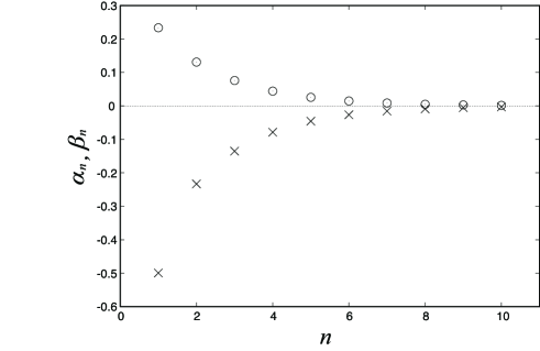
Figure 3: Numerical results of $\alpha_{n}$ (circles) and $\beta_{n}$ (crosses) for $\nu_{\rm o}=10$.

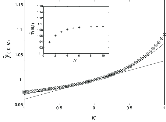
Figure 4: Numerical results of eq. (4.14) for $\nu_{\rm o}=10$ are shown for $N=1$ (solid line), $3$ (dotted line), $8$ (crosses) and $10$ (circles). The inset shows how the numerical results at $\kappa=1$ depend on $N$.

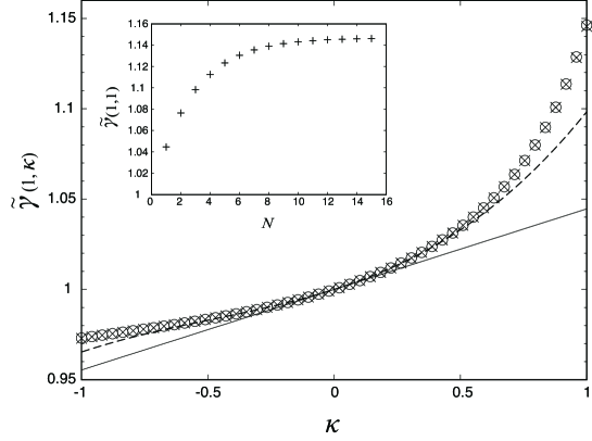
Figure 5: Numerical results of eq. (4.14) for $\nu_{\rm o}=1$ are shown for $N=1$ (solid line), $3$ (dotted line), $12$ (crosses) and $15$ (circles). The inset shows how the numerical results at $\kappa=1$ depend on $N$.

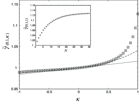
Figure 6: Numerical results of eq. (4.14) for $\nu_{\rm o}=0.1$ are shown for $N=1$ (solid line), $3$ (dotted line), $33$ (crosses) and $35$ (circles). The inset shows how the numerical results at $\kappa=1$ depend on $N$.

In calculating $[\hat{M}\tilde{A}_{n-1}]$ of eq. (4.13), we encounter the integral $\hat{M}J_{0}$, which converges but needs larger upper bound for numerical calculation. However, judging from our numerical results not shown here, we can expect well that this integral is much smaller than that of the other terms in $[\hat{M}\tilde{A}_{n-1}]$. Thus, we estimate $\hat{M}J_{0}$ by setting the upper bound to be $10000$. In estimating the value of the integral appearing explicitly in eq. (4.13), we set the option of Mathematica^® as Global Adaptive and choose the Max Error Increases as $10000$. The results for each of $\nu_{\rm o}=10,1,$ and $0.1$ represent a function of $R$, which oscillates near $R=1$ probably because the upper bounds of the integrals are changed to finite values. Instead of raising the upper bound of the integral from $10000$, we estimate the value in the limit of $R\to 1+$ by extrapolating the least-squares linear-regression equation which we obtain by using the numerical results from $R=1.001$ to $1.01$ with the intervals being $0.0001$.

For numerical calculation of eq. (4.12), we should truncate the series into the sum of the first $N$ terms, i.e.,

$$\sum_{n=0}^{N}\,\tilde{\gamma}_{n}(\nu_{\rm o})\kappa^{n}\ .$$ (4.14)

Numerical results for various values of $N$ are shown for different values of $\nu_{\rm o}$ in figs. 4, 5, and 6. The results for $N=1$ are also calculated in Fujitani (2013). In each of the figures, eq. (4.14) increases with $N$ for any nonzero $\kappa$. As shown by each inset figure, the increment of eq. (4.14) occurring at $\kappa=1$ when $N$ increases by one decreases with $N$. For $\nu_{\rm o}=10$, the increment is much smaller than $10^{-3}$ for $N\geq 9$, and we regard eq. (4.14) with $N=10$ as the value of eq. (4.12). For $\nu_{\rm o}=1$, the increment is much smaller than $10^{-3}$ for $N\geq 14$, and we regard eq. (4.14) with $N=15$ as the value of eq. (4.12). For $\nu_{\rm o}=0.1$, the increment is much smaller than $10^{-3}$ for $N\geq 34$, and we regard eq. (4.14) with $N=35$ as the value of eq. (4.12).

5 Discussion

We study the drag coefficient $\gamma$ of a liquid domain in a fluid membrane immersed in a 3D fluid. We extend the previous calculation up to the order of $\kappa$ in Fujitani (2013) to derive the recursion relations of the coefficients appearing in the series expansion of ${\tilde{\gamma}}(\nu_{\rm o},\kappa)$ with respect to $\kappa$, as shown by eqs. (4.6), (4.7), and (4.13). See eqs. (3.15) and (4.11) for the relation between $\gamma$ and ${\tilde{\gamma}}$. We numerically examine how the partial sum of eq. (4.14) depends on $N$, and find that the sums for $N=10$, $15$, and $35$ can be identified with eq. (4.12) for $\nu_{\rm o}=10$, $1$, and $0.1$, respectively.

The slopes of the solid lines in figs. 4-6 are respectively $0.0385$, $0.0446$, and $0.0156$, which agree well with the corresponding values in the column of $H\to\infty$ of Table II of Fujitani (2013). For each of $\nu_{\rm o}=10$ and $1$, the sum up to $N=1$ gives a good approximation of ${\tilde{\gamma}}$ when $|\kappa|$ is smaller than about $0.2$. For $\nu_{\rm o}=1$, the region of $\kappa$ where the sum up to $N=1$ is available is wider. When $\kappa$ is closer to unity beyond the region in each of the figures, the derivative of ${\tilde{\gamma}}$ with respect to $\kappa$ becomes larger. The drag coefficient is expected to reach a plateau value depending on the parameter as the ratio $\eta_{\rm i}/\eta_{\rm o}$ approaches zero. The circles for $\kappa<0$ in any of figs. 4-6 appears to be consistent with this expectation. It remains to be studied whether the series (4.12) is convergent or asymptotic. If the series has the radius of convergence, it would be unity, considering that the value of $\kappa$ larger than unity is meaningless. The dependence of the drag coefficient on $\kappa$ for $\kappa>0$ is not pointed out in fig. 6a of Rao and Das (2015); their $\beta$ and $\epsilon$ are respectively our $\nu_{\rm o}$ and $\kappa$. This figure is obtained from their eq. (2.7); this integral equation is discretized into a set of some thousands of simultaneous equations for numerical calculation. In the present study, to derive an equation corresponding with their integral equation above, we can sum up eq. (4.5) from $n=0$ to $\infty$ and use eq. (4.2) to derive an integral equation with respect to ${\tilde{A}}(\zeta)$. This equation contains a term involving $J_{0}$, unlike eq. (2.7) of Rao and Das (2015). This is because the third term on the lhs of eq. (3.7) is not considered in Rao and Das (2015). This term is required unless $\eta_{\rm i}$ equals $\eta_{\rm o}$, as discussed below eq. (3.7).

$\nu_{\rm o}$	$\tilde{\gamma}(\nu_{\rm o},1)$	$\tilde{\gamma}_{\rm disk}(\nu_{\rm o})$
10	1.092	1.087
1	1.146	1.137
0.1	1.128	1.123

Table 2: Comparison of our results at $\kappa=1$ with the previous results for a disk.

Let us concentrate on our results at $\kappa=1$; we have ${\tilde{\gamma}}(\nu_{\rm o},1)=1.092$, $1.146$, and $1.128$ for $\nu_{\rm o}=10$, $1$, and $0.1$, respectively, as listed in Table 2. These values are respectively in good agreement with the corresponding previous results of $\tilde{\gamma}_{\rm disk}(\nu_{\rm o})$, which are also shown in Table 1. This shows that the drag coefficient of a liquid domain reasonably approaches the one for a disk as $\eta_{\rm i}/\eta_{\rm o}$ tends to infinity. This strongly suggests that the procedure shown here is appropriate for calculating the drag coefficient of a liquid domain.

Using the procedure shown here, we can also calculate the drag coefficient of a liquid domain embedded in a fluid membrane surrounded by confined 3D fluids; this case was considered only up to the order of $\kappa$ in Fujitani (2013). The procedure can be also applied in calculating small deformation of a liquid domain in a 2D linear shear flow; it was calculated in Fujitani (2005) only for $\kappa=0$ and the stagnation flow.

Appendix A: Derivation of eqs. (3.4) and (3.5)

We introduce $\tilde{V}_{m}^{\pm}=\tilde{V}_{rm}\pm{\rm i}\tilde{V}_{\theta m}$ and define $\hat{V}_{m}^{\pm}$ as

$$\hat{V}_{m}^{\pm}(\zeta,z) = \int^{\infty}_{0}\mbox{\rm d}r\,\,rJ_{m\pm 1}(\zeta r)\tilde{V}_{m}^{\pm}(r,z)\ .$$ (A.1)

Using the transformations of eqs. (3.1) and (3.2), we can rewrite eq. (2.4) into

$$\mu(\partial^{2}_{z}-\zeta^{2})\hat{V}_{m}^{\pm} = \mp\zeta\hat{P}_{m}\ ,$$ (A.2)

$$\mu(\partial^{2}_{z}-\zeta^{2})\hat{V}_{zm} = \partial_{z}\hat{P}_{m}\ ,$$ (A.3)

$${\rm and}\quad\zeta\hat{V}^{+}_{m}-\zeta\hat{V}^{-}_{m} = -2\partial_{z}\hat{V}_{zm}\ .$$ (A.4)

As shown in Fujitani (2011), we can solve eqs. (A.2)-(A.4) together with boundary conditions, eq. (2.1) and (2.2). In particular, we have

$$\hat{P}_{\pm 1} = \frac{\zeta}{2}\left[d^{-}_{\pm 1}(\zeta)-d^{+}_{\pm 1}(\zeta)\right]\mbox{\rm e}^{-\zeta|z|}\ ,$$ (A.5)

where $d_{1}^{\pm}$ and $d_{-1}^{\pm}$ are the coefficients to be determined. From the symmetry, we have ${\hat{P}}_{1}=-{\hat{P}}_{-1}$, which leads $d_{1}^{-}-d_{1}^{+}=d_{-1}^{+}-d_{-1}^{-}$. Similarly, the symmetry of the velocity field yields $d_{1}^{+}=d_{-1}^{-}$ and $d_{1}^{-}=d_{-1}^{+}$. As discussed in Fujitani (2011) and Fujitani (2013), we find $d_{1}^{+}=d_{1}^{-}$ with the aid of the second equations of eqs. (2.4) and (2.5). Thus, we arrive at

$$\hat{P}_{m}=\hat{V}_{zm}=0\quad{\rm and}\quad\hat{V}^{\pm}_{m}(\zeta)=\frac{\mbox{\rm e}^{-\zeta|z|}}{2\mu}d^{\pm}_{m}(\zeta)\quad{\rm for}\,\,m=\pm 1\ .$$ (A.6)

Since the lhs of eq. (2.5) should be irrotational, we can eliminate $p$ from eq. (2.5) to derive

$$0=\int^{\infty}_{0}\mbox{\rm d}\zeta\,\,\zeta^{3}\,d^{+}_{1}(\zeta)\left(1+\frac{\eta}{2\mu}\zeta\right)J_{1}(\zeta r)\ ,$$ (A.7)

for $0\leq r<a$ and $a<r$. In these regions, respectively, $\eta$ equals $\eta_{\rm i}$ and $\eta_{\rm o}$. Equation (A.7) yields eqs. (3.4) and (3.5) with $A(\zeta)$ being defined as

$$A(\zeta)=2\zeta(1+\nu_{\rm o}\zeta)\,d_{1}^{+}\left({\zeta\over a}\right)\ .$$ (A.8)

Appendix B: Derivation of the recursion equations

We expand $c_{1}$ and $c_{2}$ in eq. (3.9) with respect to $\kappa$ as

$$c_{1}={2\mu a^{2}U\over Y_{0}(\nu_{\rm o})}\sum_{n=0}^{\infty}\alpha_{n}^{\sharp}\kappa^{n}\quad{\rm and}\quad c_{2}={2\mu a^{2}U\over Y_{0}(\nu_{\rm o})}\sum_{n=0}^{\infty}\beta_{n}\kappa^{n}\ ,$$ (B.1)

where $\alpha^{\sharp}_{n}$ and $\beta_{n}$ are the expansion coefficients independent of $\kappa$. Because of eq. (3.14), we have $\alpha^{\sharp}_{0}=1$. Substituting eqs. (4.1) and (4.2) into eq. (3.9) yields eq. (4.5), where $\alpha_{n}$ is given by

$$\alpha_{n} = \alpha^{\sharp}_{n}-\int^{\infty}_{0}{\rm d}\xi\frac{\xi J_{0}(\xi)}{1+\nu_{\rm o}\xi}{\tilde{A}}_{n-1}(\xi)\ .$$ (B.2)

The Fourier transform of $\tau_{r\theta}$ is defined in the same way as in eq. (3.1). For $m=1$, we have

$$\tilde{\tau}_{r\theta 1}=\frac{-\mbox{\rm i}\eta}{4\mu a^{3}}\int^{\infty}_{0}\mbox{\rm d}\zeta\,\frac{\zeta J_{2}^{\prime}(\zeta R)A(\zeta)}{1+\nu_{\rm o}\zeta}\ ,$$ (B.3)

which comes from eqs. (2.24), (2.41), and (3.13) of Fujitani (2013). Substituting eqs. (4.1), (4.2), and (4.5) into eq. (B.3), we use eq. (3.28) of Fujitani (2013) to find that eq. (2.3) gives

$$\sum_{n=0}^{\infty}\beta_{n}\left(-\kappa{\cal G}+\frac{1}{\nu_{\rm o}}\right)\kappa^{n}=\sum_{n=0}^{\infty}\left(\alpha_{n}{\hat{N}}{\tilde{A}}_{0}+\kappa{\hat{N}}{\hat{M}}{\tilde{A}_{n}}\right)\kappa^{n+1}\ ,$$ (B.4)

which yields eq. (4.7).

References

- Sutherland (1905) W. Sutherland, Philos. Mag. 9, 781 (1905).
- Einstein (1905) A. Einstein, Ann. Phys. (Leipzig) 322, 549 (1905).
- Happel and Brenner (1983) J. Happel and H. Brenner, in Low Reynolds number hydrodynamics (Martinus Nijhoff, 1983) p. 127.
- Stokes (1851) G. G. Stokes, Trans. Cambridge Philos. Soc. 9, 8 (1851).
- Hadamard (1911) J. S. Hadamard, C. R. Acad. Sci. Paris 152, 1735 (1911).
- Rybczynski (1911) W. Rybczynski, Bull. Acad. Sci. Cracovie Ser. A , 40 (1911).
- Lamb (1932) H. Lamb, in Hydrodynamics (Cambridge University Press, 1932) p. 609.
- Singer and Nicolson (1972) S. J. Singer and G. L. Nicolson, Science 175, 720 (1972).
- Saffman and Delbrück (1975) P. G. Saffman and M. Delbrück, Proc. Natl. Acad. Sci. USA 72, 3111 (1975).
- Saffman (1976) P. G. Saffman, J. Fluid Mech. 73, 593 (1976).
- Peters and Cherry (1982) R. Peters and R. J. Cherry, Proc. Natl. Acad. Sci. USA 79, 4317 (1982).
- Sneddon (1966) I. Sneddon, in Mixed boundary value problem in potential theory (North-Holland, 1966) Chap. 2 and 4.
- Hughes et al. (1981) B. D. Hughes, B. A. Pailthorpe, and L. R. White, J. Fluid Mech. 110, 349 (1981).
- Parton and Simons (1995) R. Parton and K. Simons, Science 269, 1398 (1995).
- Simons and Toomre (2000) K. Simons and D. Toomre, Mol. Cell Bio. 1, 31 (2000).
- Subczynski and Kusumi (2003) W. Subczynski and A. Kusumi, Biochim. Biophys. Acta 1610, 231 (2003).
- Veatch and Keller (2005) S. L. Veatch and S. L. Keller, Phys. Rev. Lett 94, 148101 (2005).
- Yanagisawa et al. (2007) M. Yanagisawa, M. Imai, T. Masui, S. Komura, and T. Ohta, Biophys. J 92, 115 (2007).
- Koker (1996) R. D. Koker, The Program in Biophysics, Ph.D. thesis, Stanford University (1996).
- Fujitani (2011) Y. Fujitani, J. Phys. Soc. Jpn. 80, 074609 (2011).
- Fujitani (2013) Y. Fujitani, J. Phys. Soc. Jpn. 82, 084403 (2013).
- Rao and Das (2015) V. L. Rao and S. L. Das, J. Fluid Mech. 779, 468 (2015).
- Pozrikidis (1992) C. Pozrikidis, in Boundary integral and singularity methods for linearized viscous flow (Cambridge University Press, 1992) Chap. 2.
- Merkel et al. (1989) R. Merkel, E. Sackmann, and E. Evans, J. Phys. (Paris) 50, 1535 (1989).
- Smeulders et al. (1990) J. B. A. F. Smeulders, C. Blom, and J. Mellema, Phys. Rev. A 42, 3483 (1990).
- Fujitani (2005) Y. Fujitani, J. Phys. Soc. Jpn. 74, 642 (2005).