The universal quantum invariant and colored ideal triangulations

Abstract.

The Drinfeld double of a finite dimensional Hopf algebra is a quasi-triangular Hopf algebra with the canonical element as the universal $R$-matrix, and one can obtain a ribbon Hopf algebra by adding the ribbon element. The universal quantum invariant of framed links is constructed using a ribbon Hopf algebra. In that construction, a copy of the universal $R$-matrix is attached to each crossing, and invariance under the Reidemeister III move is shown by the quantum Yang-Baxter equation of the universal $R$-matrix. On the other hand, the Heisenberg double of a finite dimensional Hopf algebra has the canonical element (the $S$-tensor) satisfying the pentagon relation. In this paper we reconstruct the universal quantum invariant using the Heisenberg double, and extend it to an invariant of equivalence classes of colored ideal triangulations of $3$-manifolds up to colored moves. In this construction, a copy of the $S$-tensor is attached to each tetrahedron, and invariance under the colored Pachner $(2,3)$ moves is shown by the pentagon relation of the $S$-tensor.

1. Introduction

The universal quantum invariant [Law89, Law90, Oht93] associated to a ribbon Hopf algebra is an invariant of framed tangles in a cube which has the universal property over Reshetikhin-Turaev invariants [RT90]. The relationship between the universal quantum invariant and $3$-dimensional, global, topological properties of tangles is not well understood, mainly because of the $2$-dimensional definition using link diagrams. In this paper, we give a reconstruction of the universal quantum invariant using colored ideal triangulations of tangle complements, and give an extension of the universal quantum invariant to an invariant of equivalence classes of colored ideal triangulations of $3$-manifolds up to colored moves. We expect that our framework will become a new method to study the quantum invariants in a $3$-dimensional way.

1.1. Reconstruction and extension of the universal quantum invariant

In the theory of quantum groups there are two doubles of a finite dimensional Hopf algebra $A$. One is the Drinfeld double $D(A)$ and the other is the Heisenberg double $H(A)$. They are both isomorphic to $A^{*}\otimes A$ as vector spaces.

The Drinfeld double $D(A)$ is a quasi-triangular Hopf algebra with a canonical element $R\in D(A)^{\otimes 2}$ as the universal $R$-matrix, which satisfies the quantum Yang-Baxter equation

$$R_{12}R_{13}R_{23}=R_{23}R_{13}R_{12},$$

see e.g. [Dri87, Maj98, Maj99]. One can obtain a ribbon Hopf algebra $D(A)^{\theta}$ by adding the ribbon element $\theta$. In what follows we assume that the universal quantum invariant is associated to $D(A)^{\theta}$ for a finite dimensional Hopf algebra $A$.

The Heisenberg double $H(A)$ is a generalization of the Heisenberg algebras [Sem92, Lu94, Kap98]. Baaj-Skandalis [BS93] and Kashaev [Kash97] showed that a canonical element $S\in H(A)^{\otimes 2}$, which we call the $S$-tensor, satisfies the pentagon relation

$$S_{12}S_{13}S_{23}=S_{23}S_{12}.$$

Kashaev [Kash97] also constructed an algebra embedding $\phi\colon\thinspace D(A)\to H(A)\otimes H(A)^{\mathrm{op}}$ such that the image of the universal $R$-matrix is a product of four variants of the $S$-tensor:

(1.1) $$\phi^{\otimes 2}(R)=S_{14}^{\prime\prime}S_{13}\tilde{S}_{24}S_{23}^{\prime}\quad\in\left(H(A)\otimes H(A)^{\mathrm{op}}\right)^{\otimes 2},$$

where $S^{\prime},S^{\prime\prime}$ and $\tilde{S}$ are the images of $S$ by maps constructed from the antipode, see Theorem 3.4.

The situation (1.1) reminds us the situation of an octahedral triangulation [CKK14, Yok11, We05] of the complement of a link in $S^{3}\setminus\{\pm\infty\}$, where an octahedron consisting of four tetrahedra is associated to each crossing of a link diagram. Actually, corresponding to the formula (1.1), Kashaev [Kash95] constructed the $R$-matrix consisting of four quantum dilogarithms defined in [FK94], and gave a link invariant. Baseilhac and Benedetti [BB11] also constructed the $R$-matrix consisting of four quantum dilogarithms, each of which is associated to tetrahedron in a singular triangulation of a $3$-manifold, and they recovered Kashaev’s $R$-matrix. Hikami and Inoue [HI14, HI15] constructed the $R$-matrix consisting of four mutations in a cluster algebra. Here a mutation is associated to a flip of triangulated surface, where a flip is obtained by attaching a tetrahedron to the surface. They also recovered Kashaev’s $R$-matrix up to a gauge-transformation.

In this context, it is natural to ask if we can reconstruct the universal quantum invariant of a tangle using an octahedral triangulation of its complement, where a copy of the $S$-tensor is associated to each tetrahedron in the octahedral triangulation.

The answer is yes, and in this paper we give such a reconstruction. Here, we would like to stress that, we can construct the universal quantum invariant using the $S$-tensor by simply rewriting the universal $R$-matrix by (variants of) the $S$-tensor using $\phi^{\otimes 2}$. However, an important result is that we give a way to relate a copy of the $S$-tensor to an ideal tetrahedron in an octahedral triangulation, and a way to read these copies of the $S$-tensor to obtain the universal quantum invariant. The framework of the above reconstruction enables us to extend the universal quantum invariant to an invariant for colored singular triangulations of $3$-manifolds up to colored moves.

1.2. Universal quantum invariant as a state sum invariant with weights in a non-commutative ring

Let us explain the nature of the coloring on a singular triangulation from a viewpoint of state sum constructions.

One can obtain a state sum invariant of tangles and $3$-manifolds by associating a $6$j-symbol to each tetrahedron in a triangulation of a $3$-manifold, where the values of the $6$j-symbol on colors on the edges of a tetrahedron give a weight of the state sum [TV92, Oc94].

In the context of hyperbolic geometry, there are several attempts to construct a state sum invariant of hyperbolic links and hyperbolic $3$-manifolds, such that, to each tetrahedron one associates Faddeev and Kashaev’s quantum dilogarithm, and the values of them on the cross ratio moduli of hyperbolic ideal triangulation give weights of the state sum. The first relation between quantum state sums and hyperbolic geometry seems to be [Kash94] by Kashaev. For an odd integer $N>1$, he proposed a state sum for triangulations of pairs $(M,L)$ of a closed oriented $3$-manifold $M$ and a link $L$ in $M$, using the cyclic $6$j-symbol $R(p,q,r)$ of the Borel subalgebra of $U_{q}(sl_{2})$. He also showed that $R(p,q,r)$ is obtained from certain operators $S$ and $\Psi_{p,q,r}$ on $\mathbb{C}^{N}\otimes\mathbb{C}^{N}$, where $S$ satisfies a certain pentagon relation and $\Psi_{p,q,r}$ satisfies a version of the quantum dilogarithm identity. A semi-classical limit of this identity gives Rogers’s identity for Euler’s dilogarithm, and this fact seems to lead Kashaev to his famous conjecture about the relationship between his invariant and the hyperbolic volumes of link complements [Kash97’].

Murakami and Murakami [MM01] showed that Kashaev’s $R$-matrix is conjugate (up to scalar multiplication) to that of the colored Jones polynomial $J_{N}$ with $q=\exp\frac{2\pi i}{N}$ and an $N$-dimensional irreducible representation of $U_{q}(sl_{2})$. This result also showed that, in the case of links in the three-sphere, the Kashaev state sums lead to well-defined invariants. Murakami-Murakami’s construction could be seen as a state sum invariant with a weight associated to a crossing, consisting of four quantum dilogarithms.

Baseilhac and Benedetti [BB04, BB05, BB07, BB11] constructed quantum hyperbolic invariants (QHI) for triples $(M,L,r)$, where $M$ is a compact oriented $3$-manifold, $L$ is a non-empty link in $M$, and $r$ is a flat principal bundle over $M$ with structure group $PSL(2,\mathbb{C})$. These invariants are obtained by adapting and generalizing the constructions of Kashaev, and in the case where $M$ is the three-sphere and $r$ is the trivial flat bundle, they recovered the Kashaev invariants. In [BB15], they reorganized QHI as invariants for tuples $(M,L,r,\kappa)$, where $\kappa$ is a family of cohomological classes called weights. In this version, the QHI are defined by state sums where tensors called matrix dilogarithms (related to the cyclic $6$j-symbols $R(p,q,r)$) are associated to tetrahedra in a singular triangulation. The arguments of the matrix dilogarithms are certain special systems of $N$th roots of hyperbolic shape parameters on the tetrahedra, encoding the flat bundle $r$ and the weights $\kappa$.

On the other hand, the universal quantum invariant could be seen as a state sum invariant with weights being tensors of a ribbon Hopf algebra; a weight is associated to each fundamental tangle (see Figure 2.2), especially a copy of the universal $R$-matrix is associated to each crossing, and one takes products of the weights in the order following the orientations of strands of a tangle (see Section 2.2 for the precise definition). We would like to apply this framework to a state sum construction using triangulations, i.e., our motto (framework) is:

Using an element $S$ satisfying a pentagon relation in an (non-commutative) algebra, construct a state sum invariant of $3$-manifolds by associating a copy of $S$ to each tetrahedron of a (singular) triangulation.

The state sum invariants using $6$j-symbols (resp. quantum dilogarithms) could be treated in this framework as functions, rather than as its values in $\mathbb{C}$, on colors on edges of tetrahedra (resp. cross ratio moduli of ideal tetrahedra [BB15]) and we expect to obtain those invariants from the universal quantum invariant naturally keeping this framework.

In the above framework one does not need to fix colors on the edges of a tetrahedron or cross ratio modulus of an ideal tetrahedron, and for the proof of invariance of state sums, instead of the pentagon identity of $6$j-symbols or of quantum dilogarithms, one would work with an algebraic pentagon relation. Moreover, we expect that such an invariant involves combinatorial information of a triangulation in its non-commutative algebra structure, including the consistency and the completeness conditions of ideal triangulations when we fix cross ratio moduli.

When we use a (singular) triangulation, we do not have a canonical order on the set of weights on tetrahedra in the triangulation. Thus we need to fix an order, then we naturally come to a notion of the colored singular triangulation : each tetrahedron is sticked by two strands and strands are connected globally in the triangulation. Then a copy of the $S$-tensor is associated to the two strands of each tetrahedron and we can read the copies of the $S$-tensor in the order following the orientations of the strands. Corresponding to the Pachner $(2,3)$ move and the $(0,2)$ move of singular triangulations, we define colored Pachner $(2,3)$ moves and colored $(0,2)$ moves of colored singular triangulations. The extension of the universal quantum invariant is an invariant of colored singular triangulations up to certain colored moves. In this paper these strands first arise from a tangle diagram, and then we consider strands more generally in singular triangulations of topological spaces.

1.3. Organization of this paper

Section 2 is devoted to the definition of the universal quantum invariant associated to a ribbon Hopf algebra. In Section 3, we recall the Drinfeld double $D(A)$ and the Heisenberg double $H(A)$ of a finite dimensional Hopf algebra $A$, where the universal $R$-matrix in $D(A)^{\otimes 2}$ and the $S$-tensor in $H(A)^{\otimes 2}$ satisfy the quantum Yang-Baxter equation and the pentagon equation, respectively. We also recall from [Kash97] how these elements are related via an embedding of $D(A)$ into $H(A)\otimes H(A)^{\mathrm{op}}$. In Section 4, we give a reconstruction of the universal quantum invariant using the Heisenberg double. In Section 5 we define colored diagrams and extend the universal quantum invariant to an invariant of colored diagrams up to colored moves. Section 6 and Section 7 are devoted to $3$-dimensional descriptions of the reconstruction and the extension of the universal quantum invariant. In Section 6 we define colored singular triangulations of topological spaces. The universal quantum invariant can be considered as an invariant of the colored singular triangulations. In Section 7 we define colored ideal triangulations of tangle complements arising from octahedral triangulations, which have been studied in e.g., [CKK14, Yok11] in the context of the hyperbolic geometry.

1.4. Acknowledgments

This work was partially supported by JSPS KAKENHI Grant Number 15K17539. The author is deeply grateful to Kazuo Habiro and Tomotada Ohtsuki for helpful advice and encouragement. She would like also to thank Stéphane Baseilhac, Riccardo Benedetti, Naoya Enomoto, Stavros Garoufalidis, Rei Inoue, Rinat Kashaev, Akishi Kato, Seonhwa Kim, Thang Le and Yuji Terashima for their helpful discussions and comments.

2. Universal quantum invariant

In this paper, a tangle means a proper embedding in a cube $[0,1]^{3}$ of a compact, oriented $1$-manifold, whose boundary points are on the two parallel lines $[0,1]\times\{0,1\}\times\{1/2\}$. A tangle diagram is a diagram of a tangle obtained from the projection $p\colon\thinspace(x,y,z)\mapsto(x,y,0)$ to the $(x,y)$-plane, see Figure 2.1. A framed tangle is a tangle equipped with a trivialization of its normal tangent bundle, which is presented in a diagram by the blackboard framing.

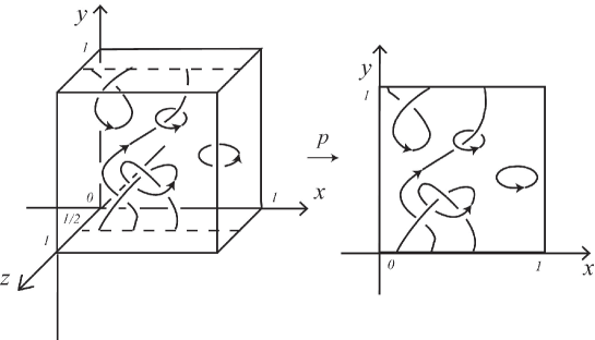
Figure 2.1. A tangle and its diagram

2.1. Ribbon Hopf algebras

Let $(A,\eta_{A},m_{A},\varepsilon_{A},\Delta_{A},\gamma_{A})$ be a finite dimensional Hopf algebra over a field $k$, with $k$-linear maps

$$\eta_{A} \colon\thinspace k\to A,$$

$$\varepsilon_{A} \colon\thinspace A\to k,$$

$$m_{A} \colon\thinspace A\otimes A\to A,$$

$$\Delta_{A} \colon\thinspace A\to A\otimes A,$$

$$\gamma_{A} \colon\thinspace A\to A,$$

which are called unit, counit, multiplication, comultiplication, and antipode, respectively. For simplicity we will omit the subscript $A$ of each map above when there is no confusion.

For distinct integers $1\leq j_{1},\ldots,j_{m}\leq l$ and $x=\sum x_{1}\otimes\cdots\otimes x_{m}\in A^{\otimes m}$, we use the notation

(2.1) $$x^{(l)}_{j_{1}\ldots j_{m}}=\sum(x_{1})_{j_{1}}\cdots(x_{m})_{j_{m}}\in A^{\otimes l},$$

where $(x_{i})_{j_{i}}$ represents the element in $A^{\otimes l}$ obtained by placing $x_{i}$ on the $j_{i}$th tensorand, i.e.,

$$(x_{i})_{j_{i}}=1\otimes\cdots\otimes x_{i}\otimes\cdots\otimes 1,$$

where $x_{i}$ is at the ${j_{i}}$th position. For example, for $x=\sum x_{1}\otimes x_{2}\otimes x_{3},$ we have $x^{(3)}_{312}=\sum x_{2}\otimes x_{3}\otimes x_{1}$. Abusing the notation, we will omit the superscript of $x^{(l)}_{j_{1}\ldots j_{m}}$ as $x_{j_{1}\ldots j_{m}}$.

For $k$-modules $V,W$, we define the symmetry map

(2.2) $$\tau_{V,W}\colon\thinspace V\otimes W\to W\otimes V,\quad a\otimes b\mapsto b\otimes a.$$

A quasi-triangular Hopf algebra $(A,\eta,m,\varepsilon,\Delta,\gamma,R)$ is a Hopf algebra $(A,\eta,m,\varepsilon,\Delta,\gamma)$ with an invertible element $R\in A^{\otimes 2}$, called the universal $R$-matrix, such that

$$\Delta^{\mathrm{op}}(x)=R\Delta(x)R^{-1}\quad\text{for }x\in A,$$

$$(\Delta\otimes 1)(R)=R_{13}R_{23},\quad(1\otimes\Delta)(R)=R_{13}R_{12},$$

where $\Delta^{\mathrm{op}}=\tau_{A,A}\circ\Delta$.

A ribbon Hopf algebra $(A,\eta,m,\varepsilon,\Delta,\gamma,R,\textbf{r})$, see e.g., [Kash95], is a quasi-triangular Hopf algebra $(A,\eta,m,\varepsilon,\Delta,\gamma,R)$ with a central, invertible element $\textbf{r}\in A$, called ribbon element, such that

$$\textbf{r}^{2}=u\gamma(u),\quad\gamma(\textbf{r})=\textbf{r},\quad\varepsilon(\textbf{r})=1,\quad\Delta(\textbf{r})=(R_{21}R)^{-1}(\textbf{r}\otimes\textbf{r}),$$

where

(2.3) $$u=\sum S(\beta)\alpha$$

with $R=\sum\alpha\otimes\beta$.

2.2. Universal quantum invariant for framed tangles

In this section, we recall the universal quantum invariant [Oht93, Law89, Law90] for framed tangles associated to a ribbon Hopf algebra $(A,\eta,m,\varepsilon,\Delta,\gamma,R,\textbf{r})$.

Let $T=T_{1}\cup\cdots\cup T_{n}$ be an $n$-component, framed, ordered tangle.

Set

$$N=\mathrm{Span}_{k}\{ab-ba\ |\ a,b\in A\}\subset A.$$

For $i=1,\ldots,n$, let

$$A_{i}=\begin{cases}A\quad&\text{if}\quad\partial T_{i}\not=\emptyset,\\ A/N\quad&\text{if}\quad\partial T_{i}=\emptyset.\end{cases}$$

We define the universal quantum invariant $J(T)\in A_{1}\otimes\cdots\otimes A_{n}$ in three steps as follows. We follow the notation in [Suz12].

Step 1. Choose a diagram. We choose a diagram $D$ of $T$ which is obtained by pasting, horizontally and vertically, copies of the fundamental tangles depicted in Figure 2.2.

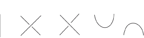
Figure 2.2. Fundamental tangles, where the orientation of each strand is arbitrary

Step 2. Attach labels. We attach labels on the copies of the fundamental tangles in the diagram, following the rule described in Figure 2.3, where each $\gamma^{\prime}$ should be replaced with $\gamma$ if the string is oriented upwards, and with the identity otherwise. We do not attach any label to the other copies of fundamental tangles, i.e., to a straight strand and to a local maximum or minimum oriented from right to left.

Figure 2.3. How to place labels on the fundamental tangles

Step 3. Read the labels. We define the $i$th tensorand of $J({D})$ as the product of the labels on the $i$th component of $D$, where the labels are read off along $T_{i}$ reversing the orientation, and written from left to right. Here, if $T_{i}$ is a closed component, then we choose arbitrary point $p_{i}$ on $T_{i}$ and read the label from $p_{i}$. The labels on the crossings are read as in Figure 2.4.

Figure 2.4. How to read the labels on crossings, where $R^{-1}=\sum\alpha^{-}\otimes\beta^{-}$

As is well known [Oht93], $J(T):=J(D)$ does not depend on the choice of the diagram and the base points $p_{i}$, and thus defines an isotopy invariant of tangles.

Figure 2.5. (a) A tangle diagram $C$, (b) The label put on $C$

For example, for the tangle $C=C_{1}\cup C_{2}$ shown in Figure 2.5, we have

(2.4) $$J({C}) =\sum\gamma(\alpha)\gamma(\beta^{\prime})\otimes\alpha^{\prime}\beta,$$

where $R=\sum\alpha\otimes\beta=\sum\alpha^{\prime}\otimes\beta^{\prime}.$

3. Drinfeld double and Heisenberg double

Let $(A,\eta,m,\varepsilon,\Delta,\gamma)$ be a finite dimensional Hopf algebra. Let $A^{*}=\mathrm{Hom}_{k}(A,k)$. Define the pairing

(3.1) $$\langle\ ,\ \rangle\colon\thinspace A^{*}\otimes A\to k,\quad f\otimes x\mapsto f(x),$$

and extend it to

$$\langle\ ,\ \rangle\colon\thinspace(A^{*})^{\otimes n}\otimes A^{\otimes n}\to k,$$

for $n\geq 1$, by

$$\langle f_{1}\otimes\cdots\otimes f_{n},x_{1}\otimes\cdots\otimes x_{n}\rangle=\langle f_{1},x_{1}\rangle\cdots\langle f_{n},x_{n}\rangle.$$

Then the dual Hopf algebra

$$A^{*}=(A^{*},\eta_{A^{*}}=\varepsilon^{*},m_{A^{*}}=\Delta^{*},\varepsilon_{A^{*}}=\eta^{*},\Delta_{A^{*}}=m^{*},\gamma_{A^{*}}=\gamma^{*})$$

is defined using the transposes of the morphisms of $A$, i.e., is defined uniquely by

$$\langle\varepsilon^{*}(a),x\rangle =a\varepsilon(x),\quad a\in k,x\in A,$$

$$\langle\Delta^{*}(f\otimes g),x\rangle =\langle f\otimes g,\Delta(x)\rangle,\quad f,g\in A^{*},x\in A,$$

$$\eta^{*}(f)a =\langle f,\eta(a)\rangle,\quad f\in A^{*},a\in k,$$

$$\langle m^{*}(f),x\otimes y\rangle =\langle f,m(x\otimes y)\rangle,\quad f\in A^{*},x,y\in A,$$

$$\langle\gamma^{*}(f),x\rangle =\langle f,\gamma(x)\rangle,\quad f\in A^{*},x\in A.$$

3.1. Drinfeld double and Yang-Baxter equation

For any finite dimensional Hopf algebra with invertible antipode, the Drinfeld quantum double construction gives a quasi-triangular Hopf algebra [Dri87]. Here, we follow the notation in [Kass95].

Let $(A,\eta,m,\varepsilon,\Delta,\gamma,\gamma^{-1})$ be a finite dimensional Hopf algebra with invertible antipode, $A^{\mathrm{op}}=(A,\eta,m^{\mathrm{op}},\varepsilon,\Delta,\gamma^{-1},\gamma)$ the opposite Hopf algebra and $(A^{\mathrm{op}})^{*}=(A^{*},\varepsilon^{*},\Delta^{*},\eta^{*},(m^{\mathrm{op}})^{*},(\gamma^{-1})^{*},\gamma^{*})$ the dual of the opposite Hopf algebra, where $m^{\mathrm{op}}=m\circ\tau_{A,A}$. For simplicity, we set

$$\bar{\gamma}=\gamma^{-1}.$$

Let $\Delta^{(0)}=\mathop{\mathrm{id}}\nolimits$ and $\Delta^{(n)}=(\Delta\otimes 1^{\otimes n-1})\Delta^{(n-1)}$ for $n\geq 1$. In what follows, for $x\in A$ or $x\in A^{*}$, we use the notation

$$\Delta(x)=\Delta^{(1)}(x) =\sum x^{\prime}\otimes x^{\prime\prime}=\sum x^{(1)}\otimes x^{(2)},$$

$$(\Delta\otimes 1)\Delta(x)=\Delta^{(2)}(x) =\sum x^{\prime}\otimes x^{\prime\prime}\otimes x^{\prime\prime\prime}=\sum x^{(1)}\otimes x^{(2)}\otimes x^{(3)},$$

$$\Delta^{(n)}(x) =\sum x^{(1)}\otimes\cdots\otimes x^{(n+1)},$$

for $n\geq 3$. We have

$$(m^{\mathrm{op}})^{*}(f)=\Delta^{\mathrm{op}}(f)=\sum f^{\prime\prime}\otimes f^{\prime}$$

for $f\in(A^{\mathrm{op}})^{*}$.

There is a unique left action

$$A\otimes(A^{\mathrm{op}})^{*}\to(A^{\mathrm{op}})^{*},\quad a\otimes f\mapsto a\cdot f,$$

such that

$$\langle a\cdot f,x\rangle=\sum\langle f,\bar{\gamma}(a^{\prime\prime})xa^{\prime}\rangle,$$

for $a,x\in A$ and $f\in(A^{\mathrm{op}})^{*}$, which induces the left $A$-module coalgebra structure on $(A^{\mathrm{op}})^{*}$. Also, there is a unique right action

$$A\otimes(A^{\mathrm{op}})^{*}\to A,\quad a\otimes f\mapsto a^{f},$$

such that

$$a^{f}=\sum f(\bar{\gamma}(a^{\prime\prime\prime})a^{\prime})a^{\prime\prime}$$

for $a\in A$ and $f\in(A^{\mathrm{op}})^{*}$, which induces the right $(A^{\mathrm{op}})^{*}$-module coalgebra structure on $A$.

The Drinfeld double

$$D(A)=((A^{\mathrm{op}})^{*}\otimes A,\eta_{D(A)},m_{D(A)},\varepsilon_{D(A)},\Delta_{D(A)},\gamma_{D(A)},R)$$

is the quasi-triangular Hopf algebra defined as the bicrossed product of $A$ and $(A^{\mathrm{op}})^{*}$. Its unit, counit, and comultiplication are given by these of $(A^{\mathrm{op}})^{*}\otimes A$, i.e., we have

$$\eta_{D(A)}(1) =\eta_{(A^{\mathrm{op}})^{*}\otimes A}(1)=1\otimes 1,$$

$$\varepsilon_{D(A)}(f\otimes a) =\varepsilon_{(A^{\mathrm{op}})^{*}\otimes A}(f\otimes a)=f(1)\varepsilon(a),$$

$$\Delta_{D(A)}(f\otimes a) =\Delta_{(A^{\mathrm{op}})^{*}\otimes A}(f\otimes a)=\sum f^{\prime\prime}\otimes a^{\prime}\otimes f^{\prime}\otimes a^{\prime\prime},$$

for $a\in A$ and $f\in(A^{\mathrm{op}})^{*}$. Its multiplication is given by

(3.2) $$m_{D(A)}\left((f\otimes a)\otimes(g\otimes b)\right) =\sum f(a^{\prime}\cdot g^{\prime\prime})\otimes a^{\prime\prime g^{\prime}}b$$

(3.3) $$=\sum fg(\bar{\gamma}(a^{\prime\prime\prime})?a^{\prime})\otimes a^{\prime\prime}b,$$

for $a,b\in A$ and $f,g\in(A^{\mathrm{op}})^{*}$, where the question mark $?$ denotes a place of the variable. Its antipode is given by

$$\gamma_{D(A)}(f\otimes a) =\sum\gamma(a^{\prime\prime})\cdot\bar{\gamma}^{*}(f^{\prime})\otimes\gamma(a^{\prime})^{\bar{\gamma}^{*}(f^{\prime\prime})},$$

for $a\in A$ and $f\in(A^{\mathrm{op}})^{*}$.

Fix a basis $\{e_{a}\}_{a\in\mathcal{I}}$ of $A$ and its dual basis $\{e^{a}\}_{a\in\mathcal{I}}$ of $A^{*}$. The universal $R$-matrix is defined as the canonical element

$$R=\sum_{a}(1\otimes e_{a})\otimes(e^{a}\otimes 1)\in D(A)\otimes D(A).$$

3.2. Heisenberg double and pentagon relation

Let $A$ be a finite dimensional Hopf algebra with an invertible antipode as in the previous section. The Heisenberg double

$$H(A)=(A^{*}\otimes A,\eta_{H(A)},m_{H(A)})$$

is the algebra with the unit $\eta_{H(A)}(1)=\eta_{A^{*}\otimes A}(1)=1\otimes 1$ and the multiplication

(3.4) $$m_{H(A)}\left((f\otimes a)\otimes(g\otimes b)\right) =\sum fg(?a^{\prime})\otimes a^{\prime\prime}b,$$

for $a,b\in A$ and $f,g\in(A^{\mathrm{op}})^{*}$.

Kashaev showed the following.

Theorem 3.1 (Kashaev [Kash97]).

The canonical element

$$S=\sum_{a}(1\otimes e_{a})\otimes(e^{a}\otimes 1)\in H(A)\otimes H(A)$$

satisfies the pentagon relation

(3.5) $$S_{12}S_{13}S_{23}=S_{23}S_{12}\quad\in H(A)^{\otimes 3}.$$

3.3. Drinfeld double and Heisenberg double

Let

$$H(A^{*})=(A\otimes A^{*},\eta_{H(A^{*})},m_{H(A^{*})})$$

be the Heisenberg double of the dual Hopf algebra $A^{*}$ of $A$, where we identify $(A^{*})^{*}$ and $A$ in the standard way.

Set $A^{\mathrm{opcop}}=(A,\eta,m^{\mathrm{op}},\varepsilon,\Delta^{\mathrm{op}},\gamma,\gamma^{-1})$. We have the following lemma.

Lemma 3.2.

The algebras $H(A^{*})$ and $H(A)^{\mathrm{op}}$ are isomorphic via the unique isomorphism $\Gamma\circ\tau$ such that

$$\tau=\tau_{A^{*},A}\colon\thinspace H(A^{*})\to H(A^{\mathrm{opcop}})^{\mathrm{op}},\quad x\otimes f\mapsto f\otimes x,$$

$$\Gamma=\bar{\gamma}^{*}\otimes\gamma\colon\thinspace H(A^{\mathrm{opcop}})^{\mathrm{op}}\to H(A)^{\mathrm{op}},\quad f\otimes x\mapsto\bar{\gamma}^{*}(f)\otimes\gamma(x).$$

Proof.

We have

$$\tau(x\otimes f)\cdot_{H(A^{\mathrm{opcop}})^{\mathrm{op}}}\tau(y\otimes g)= \left(f\otimes x\right)\cdot_{H(A^{\mathrm{opcop}})^{\mathrm{op}}}\left(g\otimes y\right)$$

$$= \left(g\otimes y\right)\cdot_{H(A^{\mathrm{opcop}})}\left(f\otimes x\right)$$

$$= \sum g\cdot_{(A^{*})^{\mathrm{op}}}\langle f,?\cdot_{A^{\mathrm{op}}}y^{\prime\prime}\rangle\otimes y^{\prime}\cdot_{A^{\mathrm{op}}}x$$

$$= \sum\langle f,y^{\prime\prime}?\rangle g\otimes xy^{\prime}$$

$$= \sum\langle f^{\prime},y^{\prime\prime}\rangle f^{\prime\prime}g\otimes xy^{\prime}$$

$$= \sum f^{\prime\prime}g\otimes xy^{\prime}\langle f^{\prime},y^{\prime\prime}\rangle$$

$$= \sum\tau\left(xy^{\prime}\langle f^{\prime},y^{\prime\prime}\rangle\otimes f^{\prime\prime}g\right)$$

$$= \sum\tau\left(x\langle?f^{\prime},y\rangle\otimes f^{\prime\prime}g\right)$$

$$= \tau\left((x\otimes f)\cdot_{H(A^{*})}(y\otimes g)\right),$$

and we have

$$\Gamma(f\otimes x)\cdot_{H(A)^{\mathrm{op}}}\Gamma(g\otimes y)= \left(\bar{\gamma}^{*}(f)\otimes\gamma(x)\right)\cdot_{H(A)^{\mathrm{op}}}\left(\bar{\gamma}^{*}(g)\otimes\gamma(y)\right)$$

$$= \left(\bar{\gamma}^{*}(g)\otimes\gamma(y)\right)\cdot_{H(A)}\left(\bar{\gamma}^{*}(f)\otimes\gamma(x)\right)$$

$$= \sum\bar{\gamma}^{*}(g)\langle\bar{\gamma}^{*}(f),?\gamma(y)^{\prime}\rangle\otimes\gamma(y)^{\prime\prime}\gamma(x)$$

$$= \sum\bar{\gamma}^{*}(g)\bar{\gamma}^{*}(f)^{\prime}\langle\bar{\gamma}^{*}(f)^{\prime\prime},\gamma(y)^{\prime}\rangle\otimes\gamma(y)^{\prime\prime}\gamma(x)$$

$$= \sum\bar{\gamma}^{*}(g)\bar{\gamma}^{*}(f^{\prime\prime})\langle\bar{\gamma}^{*}(f^{\prime}),\gamma(y^{\prime\prime})\rangle\otimes\gamma(y^{\prime})\gamma(x)$$

$$= \sum(\bar{\gamma}^{*}\otimes\gamma)\left(\langle f^{\prime},y^{\prime\prime}\rangle f^{\prime\prime}g\otimes xy^{\prime}\right)$$

$$= \sum(\bar{\gamma}^{*}\otimes\gamma)\left(\langle f,y^{\prime\prime}?\rangle g\otimes xy^{\prime}\right)$$

$$= \sum\Gamma\left(g\cdot_{(A^{*})^{\mathrm{op}}}\langle f,?\cdot_{A^{\mathrm{op}}}y^{\prime\prime}\rangle\otimes y^{\prime}\cdot_{A^{\mathrm{op}}}x\right)$$

$$= \Gamma\left((g\otimes y)\cdot_{H(A^{\mathrm{opcop}})}(f\otimes x)\right)$$

$$= \Gamma\left((f\otimes x)\cdot_{H(A^{\mathrm{opcop}})^{\mathrm{op}}}(g\otimes y)\right),$$

which completes the proof. ∎

Set

(3.6) $$\phi(1\otimes e_{a})= \sum 1\otimes e_{a}^{\prime}\otimes 1\otimes\gamma(e_{a}^{\prime\prime})\in H(A)\otimes H(A)^{\mathrm{op}},$$

(3.7) $$\phi(e^{a}\otimes 1)= \sum(e^{a})^{\prime\prime}\otimes 1\otimes\bar{\gamma}^{*}((e^{a})^{\prime})\otimes 1\in H(A)\otimes H(A)^{\mathrm{op}}.$$

Kashaev [Kash97] stated without proof that the Drinfeld double $D(A)$ can be realized as a subalgebra in the tensor product $H(A)\otimes H(A)^{\mathrm{op}}$ of the Heisenberg double $H(A)$ and its opposite algebra $H(A)^{\mathrm{op}}$ as follows.

Theorem 3.3 (Kashaev [Kash97]).

There is a unique algebra homomorphism

(3.8) $$\phi\colon\thinspace D(A)\to H(A)\otimes H(A)^{\mathrm{op}}$$

extending (3.6) and (3.7).

We give the proof of Theorem 3.3 by showing $\phi$ explicitly.

Proof of Theorem 3.3.

We define $\phi\colon\thinspace D(A)\to H(A)\otimes H(A)^{\mathrm{op}}$ by

$$\phi =m_{H(A)\otimes H(A)^{\mathrm{op}}}\circ((1\otimes\eta)^{\otimes 2}\otimes(\eta\otimes 1)^{\otimes 2})\circ(1\otimes\bar{\gamma}^{*}\otimes 1\otimes\gamma)\circ(\Delta^{\mathrm{op}}\otimes\Delta),$$

i.e., we have

$$\phi(f\otimes x) =\sum\langle\bar{\gamma}^{*}\left(f^{\prime}\right)^{\prime\prime},\gamma(x^{\prime\prime})^{\prime}\rangle f^{\prime\prime}\otimes x^{\prime}\otimes\bar{\gamma}^{*}\left(f^{\prime}\right)^{\prime}\otimes\gamma(x^{\prime\prime})^{\prime\prime}$$

$$=\sum\langle f^{\prime},x^{\prime\prime\prime}\rangle f^{\prime\prime\prime}\otimes x^{\prime}\otimes\bar{\gamma}^{*}(f^{\prime\prime})\otimes\gamma(x^{\prime\prime}),$$

for $f\in A^{*}$ and $x\in A$.

The map $\phi$ is an algebra homomorphism as follows.

$$\phi(1\otimes x)\phi(1\otimes y) =\left(\sum 1\otimes x^{\prime}\otimes 1\otimes\gamma(x^{\prime\prime})\right)\cdot_{H(A)\otimes H(A)^{\mathrm{op}}}\left(\sum 1\otimes y^{\prime}\otimes 1\otimes\gamma(y^{\prime\prime})\right)$$

$$=\sum 1\otimes x^{\prime}y^{\prime}\otimes 1\otimes\gamma(x^{\prime\prime})\cdot_{A^{\mathrm{op}}}\gamma(y^{\prime\prime})$$

$$=\sum 1\otimes(xy)^{\prime}\otimes 1\otimes\gamma((xy)^{\prime\prime})$$

$$=\phi\left((1\otimes x)\cdot_{D(A)}(1\otimes y)\right),$$

$$\phi(f\otimes 1)\phi(g\otimes 1) =\left(\sum f^{\prime\prime}\otimes 1\otimes\bar{\gamma}^{*}(f^{\prime})\otimes 1\right)\cdot_{H(A)\otimes H(A)^{\mathrm{op}}}\left(\sum g^{\prime\prime}\otimes 1\otimes\bar{\gamma}^{*}(g^{\prime})\otimes 1\right)$$

$$=\sum f^{\prime\prime}g^{\prime\prime}\otimes 1\otimes\bar{\gamma}^{*}(f^{\prime})\cdot_{(A^{*})^{\mathrm{op}}}\bar{\gamma}^{*}(g^{\prime})\otimes 1$$

$$=\sum(fg)^{\prime\prime}\otimes 1\otimes\bar{\gamma}^{*}((fg)^{\prime})\otimes 1$$

$$=\phi\left((f\otimes 1)\cdot_{D(A)}(g\otimes 1)\right),$$

$$\phi(f\otimes 1)\phi(1\otimes x) =\left(\sum f^{\prime\prime}\otimes 1\otimes\bar{\gamma}^{*}(f^{\prime})\otimes 1\right)\cdot_{H(A)\otimes H(A)^{\mathrm{op}}}\left(\sum 1\otimes x^{\prime}\otimes 1\otimes\gamma(x^{\prime\prime})\right)$$

$$=\sum f^{\prime\prime}\otimes x^{\prime}\otimes\langle\bar{\gamma}^{*}(f^{\prime})^{\prime\prime},\gamma(x^{\prime\prime})^{\prime}\rangle\bar{\gamma}^{*}\left(f^{\prime}\right)^{\prime}\otimes\gamma(x^{\prime\prime})^{\prime\prime}$$

$$=\sum\langle f^{\prime},x^{\prime\prime\prime}\rangle f^{\prime\prime\prime}\otimes x^{\prime}\otimes\bar{\gamma}^{*}\left(f^{\prime\prime}\right)\otimes\gamma(x^{\prime\prime})$$

$$=\phi(f\otimes x)$$

$$=\phi\left((f\otimes 1)\cdot_{D(A)}(1\otimes x)\right),$$

$$\phi(1\otimes x)\phi(f\otimes 1) =\left(\sum 1\otimes x^{(1)}\otimes 1\otimes\gamma(x^{(2)})\right)\cdot_{H(A)\otimes H(A)^{\mathrm{op}}}\left(\sum f^{(2)}\otimes 1\otimes\bar{\gamma}^{*}(f^{(1)})\otimes 1\right)$$

$$=\sum\langle f^{(3)},x^{(1)}\rangle f^{(2)}\otimes x^{(2)}\otimes\bar{\gamma}^{*}\left(f^{(1)}\right)\otimes\gamma(x^{(3)})$$

$$=\sum\langle f^{(4)},x^{(1)}\rangle\varepsilon(f^{(1)})\varepsilon\left(x^{(4)}\right)f^{(3)}\otimes x^{(2)}\otimes\bar{\gamma}^{*}\left(f^{(2)}\right)\otimes\gamma(x^{(3)})$$

$$=\sum\langle f^{(4)},x^{(1)}\rangle\langle f^{(1)},\bar{\gamma}(x^{(5)})x^{(4)}\rangle f^{(3)}\otimes x^{(2)}\otimes\bar{\gamma}^{*}\left(f^{(2)}\right)\otimes\gamma(x^{(3)})$$

$$=\sum\langle f^{(5)},x^{(1)}\rangle\langle f^{(1)},\bar{\gamma}(x^{(5)})\rangle\langle f^{(2)},x^{(4)}\rangle f^{(4)}\otimes x^{(2)}\otimes\bar{\gamma}^{*}\left(f^{(3)}\right)\otimes\gamma(x^{(3)})$$

$$=\phi\left(\langle f^{(1)},\gamma(x^{(3)})\rangle\langle f^{(3)},x^{(1)}\rangle f^{(2)}\otimes x^{(2)}\right)$$

$$=\phi\left((1\otimes x)\cdot_{D(A)}(f\otimes 1)\right),$$

where the fourth identity follows from $m^{\mathrm{op}}(1\otimes\bar{\gamma})\Delta=\eta\varepsilon$.

The map $\phi$ satisfies (3.6) and (3.7) as follows.

$$\phi(1\otimes e_{a}) =\sum\langle 1,e_{a}^{\prime\prime\prime}\rangle 1\otimes e_{a}^{\prime}\otimes 1\otimes\gamma\left(e_{a}^{\prime\prime})\right).$$

$$=\sum 1\otimes e_{a}^{\prime}\otimes 1\otimes\gamma(e_{a}^{\prime\prime})$$

$$=\phi(1\otimes e_{a}),$$

$$\phi(e^{a}\otimes 1) =\sum\langle(e^{a})^{\prime},1\rangle(e^{a})^{\prime\prime\prime}\otimes 1\otimes\left(\bar{\gamma}^{*}(e^{a})^{\prime\prime}\right)\otimes 1.$$

$$=\sum(e^{a})^{\prime\prime}\otimes 1\otimes\bar{\gamma}^{*}((e^{a})^{\prime})\otimes 1$$

$$=\phi(e^{a}\otimes 1).$$

Thus we have the assertion. ∎

Set

$$\hat{R} =\phi^{\otimes 2}(R)=\sum_{a}\phi(1\otimes e_{a})\otimes\phi(e^{a}\otimes 1)$$

$$=\sum 1\otimes e_{a}^{\prime}\otimes 1\otimes\gamma(e_{a}^{\prime\prime})\otimes(e^{a})^{\prime\prime}\otimes 1\otimes\bar{\gamma}^{*}((e^{a})^{\prime})\otimes 1 \in\left(H(A)\otimes H(A)^{\mathrm{op}}\right)^{\otimes 2}.$$

Since $\phi^{\otimes 2}$ is an algebra homomorphism, the element $\hat{R}$ also satisfies the quantum Yang-Baxter equation:

(3.9) $$\hat{R}_{12}\hat{R}_{13}\hat{R}_{23}=\hat{R}_{23}\hat{R}_{13}\hat{R}_{12},$$

where we use the notation (2.1) treating $H(A)\otimes H(A)^{\mathrm{op}}$ as one algebra. If we treat $H(A)\otimes H(A)^{\mathrm{op}}$ as the tensor of $H(A)$ and $H(A)^{\mathrm{op}}$, we have

$$\hat{R}_{1234}\hat{R}_{1256}\hat{R}_{3456}=\hat{R}_{3456}\hat{R}_{1256}\hat{R}_{1234}.$$

Set

$$\tilde{e}_{a}:=\gamma(e_{a}),\quad\tilde{e}^{b}:=\bar{\gamma}^{*}(e^{b}),$$

and set

$$S^{\prime} =\sum(1\otimes\tilde{e}_{a})\otimes(e^{a}\otimes 1)\quad\in H(A)^{\mathrm{op}}\otimes H(A),$$

$$S^{\prime\prime} =\sum(1\otimes e_{a})\otimes(\tilde{e}^{a}\otimes 1)\quad\in H(A)\otimes H(A)^{\mathrm{op}},$$

$$\tilde{S} =\sum(1\otimes\tilde{e}_{a})\otimes(\tilde{e}^{a}\otimes 1)\quad\in H(A)^{\mathrm{op}}\otimes H(A)^{\mathrm{op}}.$$

Kashaev showed the following.

Theorem 3.4 (Kashaev [Kash97]).

We have

(3.10) $$\hat{R} =S_{14}^{\prime\prime}S_{13}\tilde{S}_{24}S_{23}^{\prime}\quad\in\left(H(A)\otimes H(A)^{\mathrm{op}}\right)^{\otimes 2}.$$

Proposition 3.5 (Kashaev [Kash97]).

The quantum Yang-Baxter equation (3.9) in $\left(H(A)\otimes H(A)^{\mathrm{op}}\right)^{\otimes 3}$ is a consequence of the following variations of the pentagon equation for the tensors $S,S^{\prime},S^{\prime\prime}$ and $\tilde{S}$:

(3.11) $$S_{23}S_{12}=S_{12}S_{13}S_{23},\quad S_{23}S^{\prime}_{12}=S^{\prime}_{12}S^{\prime}_{13}S_{23},$$

(3.12) $$S^{\prime\prime}_{23}S_{12}=S_{12}S^{\prime\prime}_{13}S^{\prime\prime}_{23},\quad S^{\prime\prime}_{23}S^{\prime}_{12}=S^{\prime}_{12}S^{\prime\prime}_{13}S^{\prime\prime}_{23},$$

and

(3.13) $$S^{\prime}_{23}S_{13}S^{\prime\prime}_{12}=S^{\prime\prime}_{12}S^{\prime}_{23},\quad S^{\prime}_{23}S^{\prime}_{13}\tilde{S}_{12}=\tilde{S}_{12}S^{\prime}_{23},$$

(3.14) $$\tilde{S}_{23}S^{\prime\prime}_{13}S^{\prime\prime}_{12}=S^{\prime\prime}_{12}S^{\prime\prime}_{23},\quad\tilde{S}_{23}\tilde{S}_{13}\tilde{S}_{12}=\tilde{S}_{12}\tilde{S}_{23}.$$

4. Reconstruction of the universal quantum invariant

Let $D(A)$ be the Drinfeld double of $A$. Recall from (2.3) the element $u=\sum\gamma(\beta)\alpha=\sum\bar{\gamma}^{*}(e^{a})\otimes e_{a}$ with $R=\sum\alpha\otimes\beta=\sum(1\otimes e_{a})\otimes(e^{a}\otimes 1)$. We have a ribbon Hopf algebra

$$D(A)^{\theta}=D(A)[\theta]/\left(\theta^{2}-u\gamma(u)\right)$$

with the ribbon element $\theta$ (e.g., [Kass95]).

We also consider the algebra

$$\left(H(A)\otimes H(A)^{\mathrm{op}}\right)^{\bar{\theta}}=\left(H(A)\otimes H(A)^{\mathrm{op}}\right)[\bar{\theta}]/\left(\bar{\theta}^{2}-\phi(u\gamma(u))\right),$$

and extend $\phi$ to the map

$$\phi\colon\thinspace D(A)^{\theta}\to\left(H(A)\otimes H(A)^{\mathrm{op}}\right)^{\bar{\theta}}$$

by $\phi(\theta)=\bar{\theta}$.

In this section, we define tangle invariant $J^{\prime\prime}$ using $\left(H(A)\otimes H(A)^{\mathrm{op}}\right)^{\bar{\theta}}$, which turns out to be the image of tensor power of $\phi$ of the universal invariant associated to $D(A)^{\theta}$ (Theorem 4.1).

In what follows, for simplicity, we use the notation

$$fx=f\otimes x\in A^{*}\otimes A,$$

for $f\in A^{*}$ and $x\in A$. In particular we have

$$S=\sum_{a}e^{a}\otimes e_{a},\quad S^{\prime}=\sum_{a}\tilde{e}^{a}\otimes e_{a},\quad S^{\prime\prime}=\sum_{a}e^{a}\otimes\tilde{e}_{a},\quad\tilde{S}=\sum_{a}\tilde{e}^{a}\otimes\tilde{e}_{a}.$$

4.1. Reconstruction of the universal quantum invariant using the Heisenberg double

Let $T=T_{1}\cup\cdots\cup T_{n}$ be an $n$-component, framed, ordered tangle. Similarly to Section 2.2, set

$$N_{\left(H\otimes H^{\mathrm{op}}\right)^{\bar{\theta}}} =\mathrm{Span}_{k}\{ab-ba\ |\ a,b\in\left(H(A)\otimes H(A)^{\mathrm{op}}\right)^{\bar{\theta}}\}\subset\left(H(A)\otimes H(A)^{\mathrm{op}}\right)^{\bar{\theta}}.$$

For $i=1,\ldots,n$, let

(4.1) $$\left(H(A)\otimes H(A)^{\mathrm{op}}\right)^{\bar{\theta}}_{i}=\begin{cases}(H(A)\otimes H(A)^{\mathrm{op}})^{\bar{\theta}}\quad&\text{if}\quad\partial T_{i}\not=\emptyset,\\ \left(H(A)\otimes H(A)^{\mathrm{op}}\right)^{\bar{\theta}}/N_{\left(H(A)\otimes H(A)^{\mathrm{op}}\right)^{\bar{\theta}}}\quad&\text{if}\quad\partial T_{i}=\emptyset.\end{cases}$$

Take a diagram $D$ of $T$. We define an element $J^{\prime}(D)\in\bigotimes_{i}\left(H(A)\otimes H(A)^{\mathrm{op}}\right)^{\bar{\theta}}_{i}$ modifying the definition of $J(T)$ as follows.

We duplicate $D$ and thicken the left strands following the orientation, and denote the result by $\zeta(D)$. See (a), (b) in Figure 4.1 and Figure 4.2 for examples.

Then we put labels on crossings as in Figure 4.3, where each $\gamma^{\prime}$ and each $(\bar{\gamma}^{*})^{\prime}$ should be replaced with $\gamma$ and $\bar{\gamma}^{*}$, respectively, if the string is oriented upwards, and with the identities otherwise.

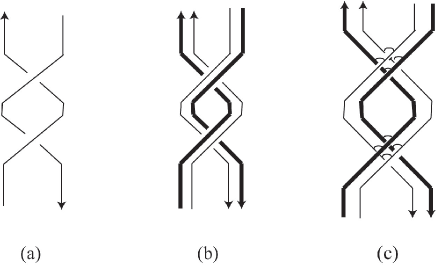
Figure 4.1. (a) A tangle $C$, (b) The diagram $\zeta(C)$, (c) Parameters for $\zeta(C)$

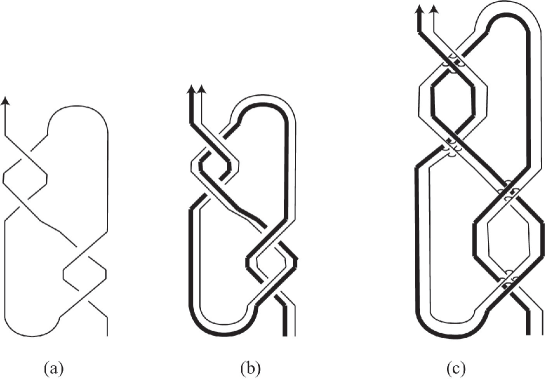
Figure 4.2. (a) A tangle $T_{41}$, (b) The diagram $\zeta(T_{41})$, (c) Parameters for $\zeta(T_{41})$

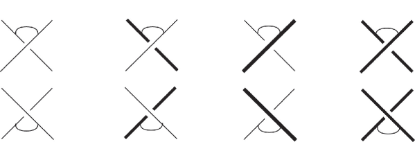
Figure 4.3. Labels on crossings

We define the $(2i-1)$st and the $2i$th tensorands of $J^{\prime}(D)$ as the product of the labels on the thin and the thick strands, respectively, obtained by duplicating $T_{i}$, where the labels are read off reversing the orientation, and written from left to right. Here, if $T_{i}$ is a closed component, then we choose a point $p$ on $T_{i}$ and denote by $p^{\prime}$ (resp. $p^{\prime\prime}$) the image of $p$ by the duplicating procedure on the thin (resp. thick) strand. We read the labels of the thin (resp. thick) strand from $p^{\prime}$ (resp. $p^{\prime\prime}$).

Let

(4.2) $$(\leftarrow)\colon\thinspace\text{\{tangle diagrams\}}\to\text{\{tangle diagrams\}},\quad D\mapsto D_{(\leftarrow)},$$

where $D_{(\leftarrow)}$ is the diagram obtained from $D$ by replacing each of and with and , respectively.

For $i=1,\ldots,n$, let $D_{i}$ be the subdiagram of $D$ corresponding to $T_{i}$. We define $d(D_{i})$ as the number of minus the number of in $D_{i}$.

Set

$$J^{\prime\prime}(D)=\left(\prod_{i}\bar{\theta}_{i}^{d(D_{i})}\right)J^{\prime}(D_{(\leftarrow)})\in\bigotimes_{i}\left(H(A)\otimes H(A)^{\mathrm{op}}\right)^{\bar{\theta}}_{i},$$

where $\bar{\theta}_{i}$ is defined following the notation (2.1).

Theorem 4.1.

We have

$$\phi^{\otimes n}\circ J(T) =J^{\prime\prime}(D)\quad\in\bigotimes_{i}\left(H(A)\otimes H(A)^{\mathrm{op}}\right)^{\bar{\theta}}_{i}.$$

If moreover $T$ is a braid, which is a $0$-framed tangle with no maxima or minima, then we have $D=D_{(\leftarrow)}$, $\prod_{i}\bar{\theta}_{i}^{d(D_{i})}=1$. Thus we have the following.

Corollary 4.2.

If $T$ is a braid, then we have

$$\phi^{\otimes n}\circ J(T)=J^{\prime}(D)\quad\in\bigotimes_{i}\left(H(A)\otimes H(A)^{\mathrm{op}}\right)_{i},$$

where $\left(H(A)\otimes H(A)^{\mathrm{op}}\right)_{i}$ is defined similarly as (4.1) using $H(A)\otimes H(A)^{\mathrm{op}}$ instead of $\left(H(A)\otimes H(A)^{\mathrm{op}}\right)^{\bar{\theta}}$.

Let $f(D_{i})=\#\text{\{positive self crossings of $D_{i}$\}}-\#\text{\{negative self crossings of $D_{i}$\}}$ be the framing of $D_{i}$. Set

$$J^{0}(D)=\left(\prod_{i}\bar{\theta}_{i}^{f(D_{i})}\right)J^{\prime}(D)\in\bigotimes_{i}\left(H(A)\otimes H(A)^{\mathrm{op}}\right)^{\bar{\theta}}_{i}.$$

We use the following lemma to prove Theorem 4.1.

Lemma 4.3.

Let $T$ be an $n$-component framed tangle, and let $T^{0}$ denote $T$ with $0$-framing. Let $D$ be a diagram of $T$. We have

$$\phi^{\otimes n}\circ J(T^{0})=J^{0}(D_{(\leftarrow)})\quad\in\bigotimes_{i}\left(H(A)\otimes H(A)^{\mathrm{op}}\right)^{\bar{\theta}}_{i}.$$

Proof.

For a positive (resp. negative) crossing $c=c_{1}\cup c_{2}$, where $c_{1}$ is the under strand, let $c^{0}$ be a tangle obtained by inserting a negative (resp. positive) kink to the bottom of $c_{1}$, see Figure 4.4 for examples. We take a diagram $D^{0}$ of $T^{0}$ obtained from $D_{(\leftarrow)}$ by replacing each self crossing $c$ by $c^{0}$ so that framings vanish.

Figure 4.4. How to insert a kink to a crossing

Since the labels on $D_{(\leftarrow)}$ to define $J^{\prime}$ are only on crossings (since there are no and ), in order to prove the assertion it is enough to show

1. $\phi^{\otimes 2}\circ J(c_{\pm})=J^{\prime}(c_{\pm})$,

2. $\phi^{\otimes 2}\circ J(c^{0}_{\pm})=\bar{\theta}^{\pm 1}_{1}J^{\prime}(c_{\pm})$,

for positive (resp. negative) crossing $c_{+}$ (resp. $c_{-}$) with each strand oriented arbitrarily.

Assume that each strand of $c_{\pm}$ is oriented downwards.

(1) follows from

$$\phi^{\otimes 2}\circ J(c_{+}) =\hat{R}_{1234}=S_{14}^{\prime\prime}S_{13}\tilde{S}_{24}S_{23}^{\prime}$$

$$=\sum_{a,b,c,d}e_{a}e_{b}\otimes\tilde{e}_{d}\tilde{e}_{c}\otimes e^{b}e^{c}\otimes\tilde{e}^{a}\tilde{e}^{d}=J^{\prime}(c_{+}),$$

$$\phi^{\otimes 2}\circ J(c_{-}) =\hat{R}^{-1}_{1234}=(S_{23}^{\prime})^{-1}(\tilde{S}_{24})^{-1}(S_{13})^{-1}(S_{14}^{\prime\prime})^{-1}$$

$$=\sum_{a,b,c,d}u_{b}u_{c}\otimes\tilde{u}_{a}\tilde{u}_{d}\otimes u^{a}u^{b}\otimes\tilde{u}^{d}\tilde{u}^{c}=J^{\prime}(c_{-}),$$

where $u_{a}$, $u^{a}$, $\tilde{u}_{a}$, $\tilde{u}^{a}$ are defined by

$$\sum_{a}u_{a}\otimes u^{a}=S^{-1}=\sum_{a}\gamma(e_{a})\otimes e^{a},\quad\sum_{a}\tilde{u}_{a}\otimes u^{a}=(S^{\prime})^{-1}=\sum_{a}\gamma(\tilde{e}_{a})\otimes e^{a},$$

$$\sum_{a}u_{a}\otimes\tilde{u}^{a}=(S^{\prime\prime})^{-1}=\sum_{a}\gamma(e_{a})\otimes\tilde{e}^{a},\quad\sum_{a}\tilde{u}_{a}\otimes\tilde{u}^{a}=\tilde{S}^{-1}=\sum_{a}\gamma(\tilde{e}_{a})\otimes\tilde{e}^{a},$$

see Figure 4.5.

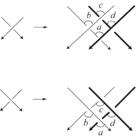
Figure 4.5. Labels on the colored diagrams $\zeta(c_{\pm})$ associated to positive and negative crossings $c_{\pm}$

Since the universal invariant of a positive (resp. negative) kink is equal to $\theta^{-1}$ (resp. $\theta$), we have $J(c_{\pm}^{0})=\theta^{\pm 1}_{1}J(c_{\pm})$. Thus (2) follows from

$$\phi^{\otimes 2}\circ J(c_{\pm}^{0}) =\phi^{\otimes 2}\left(\theta^{\pm 1}_{1}J(c_{\pm})\right)$$

$$=\bar{\theta}^{\pm 1}_{1}(\phi^{\otimes 2}\circ J)(c_{\pm})$$

$$=\bar{\theta}^{\pm 1}_{1}J^{\prime}(c_{\pm}),$$

where the last identity follows from (1).

For a crossing $c_{\pm}$ with other orientations, (1) and (2) follow similarly from

$$\phi^{\otimes 2}\circ(\gamma_{D(A)}\otimes 1)(R) =\sum_{a,b,c,d}\gamma(\tilde{e}_{c})\gamma(\tilde{e}_{d})\otimes\gamma(e_{b})\gamma(e_{a})\otimes e^{b}e^{c}\otimes\tilde{e}^{a}\tilde{e}^{d},$$

$$\phi^{\otimes 2}\circ(1\otimes\gamma_{D(A)})(R) =\sum_{a,b,c,d}e_{a}e_{b}\otimes\tilde{e}_{d}\tilde{e}_{c}\otimes\bar{\gamma}^{*}(\tilde{e}^{d})\bar{\gamma}^{*}(\tilde{e}^{a})\otimes\bar{\gamma}^{*}(e^{c})\bar{\gamma}^{*}(e^{b}),$$

$$\phi^{\otimes 2}\circ(\gamma_{D(A)}\otimes 1)(R^{-1}) =\sum_{a,b,c,d}\gamma(\tilde{u}_{d})\gamma(\tilde{u}_{a})\otimes\gamma(u_{c})\gamma(u_{b})\otimes u^{a}u^{b}\otimes\tilde{u}^{d}\tilde{u}^{c},$$

$$\phi^{\otimes 2}\circ(1\otimes\gamma_{D(A)})(R^{-1}) =\sum_{a,b,c,d}u_{b}u_{d}\otimes\tilde{u}_{a}\tilde{u}_{d}\otimes\bar{\gamma}^{*}(\tilde{u}^{c})\bar{\gamma}^{*}(\tilde{u}^{d})\otimes\bar{\gamma}^{*}(u^{b})\bar{\gamma}^{*}(u^{a}),$$

which completes the proof.

∎

Proof of Theorem 4.1.

By Lemma 4.3 we have

$$\phi^{\otimes n}\circ J(T) =\phi^{\otimes n}\left(\left(\prod_{i}\theta_{i}^{-f(D_{i})}\right)J(T^{0})\right)$$

$$=\left(\prod_{i}\bar{\theta}_{i}^{-f(D_{i})}\right)\left(\phi^{\otimes n}\circ J(T^{0})\right)$$

$$=\left(\prod_{i}\bar{\theta}_{i}^{-f(D_{i})}\right)J^{0}(D_{(\leftarrow)})$$

$$=\left(\prod_{i}\bar{\theta}_{i}^{-f(D_{i})}\right)\left(\prod_{i}\bar{\theta}_{i}^{f((D_{(\leftarrow)})_{i})}\right)J^{\prime}(D_{(\leftarrow)})$$

$$=\left(\prod_{i}\bar{\theta}_{i}^{d(D_{i})}\right)J^{\prime}(D_{(\leftarrow)}).$$

Thus we have the assertion.

∎

For the example with $C$, with the parameters as in Figure 4.1 (c), we have

$$J^{\prime}_{C}=\sum_{i_{a},i_{b},i_{c},i_{d},j_{a},j_{b},j_{c},j_{d}} \gamma(e_{i_{c}})\gamma(e_{i_{d}})\bar{\gamma}^{*}(e^{j_{d}})\bar{\gamma}^{*}(e^{j_{a}})\otimes\gamma(\tilde{e}_{i_{b}})\gamma(\tilde{e}_{i_{a}})\bar{\gamma}^{*}(\tilde{e}^{j_{c}})\bar{\gamma}^{*}(\tilde{e}^{j_{b}})$$

$$\otimes e_{j_{a}}e_{j_{b}}e^{i_{b}}e^{i_{c}}\otimes\tilde{e}_{j_{d}}\tilde{e}_{j_{c}}\tilde{e}^{i_{a}}\tilde{e}^{i_{d}}.$$

For the example with $T_{41}$, with the parameters as in Figure 4.2 (c), we have

$$J^{\prime}_{{T_{41}}}= \sum_{i_{a},i_{b},i_{c},i_{d},j_{a},j_{b},j_{c},j_{d},k_{a},k_{b},k_{c},k_{d},l_{a},l_{b},l_{c},l_{d}}\bar{\gamma}^{*}(u^{i_{c}})\bar{\gamma}^{*}(u^{i_{d}})\gamma(u_{j_{d}})\gamma(u_{j_{a}})e^{l_{b}}e^{l_{c}}e_{k_{a}}e_{k_{b}}$$

$$\times u^{j_{a}}u^{j_{b}}u_{i_{b}}u_{i_{c}}\bar{\gamma}^{*}(e^{k_{d}})\bar{\gamma}^{*}(e^{k_{a}})\gamma(e_{l_{c}})\gamma(e_{l_{d}})$$

$$\otimes\bar{\gamma}^{*}(\tilde{u}^{i_{b}})\bar{\gamma}^{*}(\tilde{u}^{i_{a}})\gamma(\tilde{u}_{j_{c}})\gamma(\tilde{u}_{j_{b}})\tilde{e}^{l_{a}}\tilde{e}^{l_{d}}\tilde{e}_{k_{d}}\tilde{e}_{k_{c}}$$

$$\times\tilde{u}^{j_{d}}\tilde{u}^{j_{c}}\tilde{u}_{i_{a}}\tilde{u}_{i_{d}}\bar{\gamma}^{*}(\tilde{e}^{k_{c}})\bar{\gamma}^{*}(\tilde{e}^{k_{b}})\gamma(\tilde{e}_{l_{b}})\gamma(\tilde{e}_{l_{a}}).$$

5. Extension of the universal quantum invariant to an invariant for colored diagrams

In this section we define colored diagrams and extend the map $J^{\prime}$ to an invariant for colored diagrams up to colored moves.

5.1. Colored diagrams and an extension of $J^{\prime}$.

In what follows, we consider also a virtual crossing as in Figure 5.1, which we call a symmetry. By a crossing we mean only a real crossing.

A colored diagram $Z$ is a virtual tangle diagram consisting of thin strands and thick strands, which is obtained by pasting, horizontally and vertically, copies of fundamental tangle diagrams in Figure 2.2 and copies of the symmetry, where the thickness of each strand are arbitrary.

Figure 5.1. A symmetry, where the orientation of each strand is arbitrary

Let $\mathcal{CD}$ be the set of colored diagrams. For $\mu=(\mu_{1}\ldots,\mu_{n}),\nu=(\nu_{1},\ldots,\nu_{n})\in\{\pm\}^{n}$, we denote by

$$\mathcal{CD}(\mu;\nu)\subset\mathcal{CD}$$

the set of $n$-component colored diagrams $Z=Z_{1}\cup\cdots\cup Z_{n}$ such that

$$Z_{i}\text{ is thin }\Leftrightarrow\mu_{i}=+, \quad Z_{i}\text{ is thick }\Leftrightarrow\mu_{i}=-,$$

$$\partial Z_{i}\not=\emptyset\Leftrightarrow\nu_{i}=+, \quad\partial Z_{i}=\emptyset\Leftrightarrow\nu_{i}=-.$$

For $i=1,\ldots,n$, set

$$H(A)_{i}^{+} =H(A),\quad H(A)_{i}^{-}=H(A)/N_{H(A)},$$

$$(H(A)^{\mathrm{op}})_{i}^{+} =H(A)^{\mathrm{op}},\quad(H(A)^{\mathrm{op}})_{i}^{-}=H(A)^{\mathrm{op}}/N_{H(A)^{\mathrm{op}}}.$$

We define the map

$$J^{\prime}\colon\thinspace\mathcal{CD}(\mu;\nu)\to\bigotimes_{\mu_{i}=+}H(A)_{i}^{\nu_{i}}\bigotimes_{\mu_{j}=-}(H(A)^{\mathrm{op}})_{j}^{\nu_{j}}$$

in a similar way to the definition of $J^{\prime}$ in Section 4, i.e., by putting the labels on the crossings as in Figure 4.3, not putting label for other fundamental tangle diagrams, and by taking the product of the labels.

5.2. Colored moves

We define several moves on colored diagrams as follows.

The colored Pachner $(2,3)$ moves are defined in Figure 5.2. Note that each colored Pachner $(2,3)$ move involves a symmetry, and thus is not the Reidemeister III move on tangle diagrams.

The colored $(0,2)$ moves are defined in Figure 5.3.

The symmetry moves are defined in Figure 5.4.

The planar isotopies are defined in Figure 5.5.

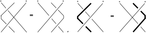
Figure 5.2. The colored Pachner $(2,3)$ moves, where the orientation and the thickness of each $*$-marked strand are arbitrary

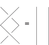
Figure 5.3. The colored $(0,2)$ moves, where the orientation and the thickness of each strand are arbitrary

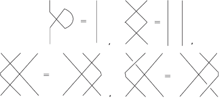
Figure 5.4. The symmetry moves, where the orientation and thickness of each strand are arbitrary

Figure 5.5. The planar isotopies, where the orientation and thickness of each strand are arbitrary

We call each of the above move a colored move.

Let $\sim_{c}$ be the equivalence relation on the set of colored diagrams generated by all colored moves.

Similarly, let $\sim^{\prime}_{c}$ be the equivalence relation on the set of colored diagrams generated by colored moves except for the moves in Figure 5.6.

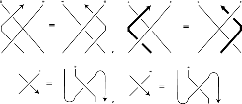
Figure 5.6. The colored moves which are not in generators for $\sim^{\prime}_{c}$, where the orientation and the thickness of each $*$-marked strand are arbitrary

We have the following.

Theorem 5.1.

The map $J^{\prime}$ is an invariant under $\sim^{\prime}_{c}$. If $\gamma^{2}=1$, then the map $J^{\prime}$ is also an invariant under $\sim_{c}$.

Proof.

Let $Z$ and $Z^{\prime}$ be two colored diagram.

If $Z$ and $Z^{\prime}$ are related by a colored Pachner $(2,3)$ move with strands oriented downwards, then $J^{\prime}(Z)=J^{\prime}(Z^{\prime})$ follows from the pentagon relations (3.11)–(3.14). If some $*$-marked strands are upwards, then $J^{\prime}(Z)=J^{\prime}(Z^{\prime})$ follows from the pentagon relations, after applying the antipode on each tensorand corresponding to an upward strand.

If $Z$ and $Z^{\prime}$ are related by a colored $(0,2)$ move, then $J^{\prime}(Z)=J^{\prime}(Z^{\prime})$ follows from the invertibility of $S$, $S^{\prime}$, $S^{\prime\prime}$, and $\tilde{S}$.

If $Z$ and $Z^{\prime}$ are related by a symmetry move, or by a planar isotopy which does not involve a crossing, then it is easy to see $J^{\prime}(Z)=J^{\prime}(Z^{\prime})$.

Let us assume that $Z$ and $Z^{\prime}$ are related by a planar isotopy which involves a crossing. If the planar isotopy is not in Figure 5.6, then $J^{\prime}(Z)=J^{\prime}(Z^{\prime})$ follows from

$$(\gamma\otimes 1)(S)=S^{-1},\quad(1\otimes\bar{\gamma}^{*})(S^{-1})=S,\quad(\gamma\otimes\bar{\gamma}^{*})(S)=S\quad\in H(A)\otimes H(A),$$

$$(\gamma\otimes 1)(S^{\prime})=(S^{\prime})^{-1},\quad(1\otimes\bar{\gamma}^{*})((S^{\prime})^{-1})=S^{\prime},\quad(\gamma\otimes\bar{\gamma}^{*})(S^{\prime})=S^{\prime}\quad\in H(A)^{\mathrm{op}}\otimes H(A),$$

$$(\gamma\otimes 1)(S^{\prime\prime})=(S^{\prime\prime})^{-1},\quad(1\otimes\bar{\gamma}^{*})((S^{\prime\prime})^{-1})=S^{\prime\prime},\quad(\gamma\otimes\bar{\gamma}^{*})(S^{\prime\prime})=S^{\prime\prime}\quad\in H(A)\otimes H(A)^{\mathrm{op}},$$

$$(\gamma\otimes 1)(\tilde{S})=\tilde{S}^{-1},\quad(1\otimes\bar{\gamma}^{*})(\tilde{S}^{-1})=\tilde{S},\quad(\gamma\otimes\bar{\gamma}^{*})(\tilde{S})=\tilde{S}\quad\in H(A)^{\mathrm{op}}\otimes H(A)^{\mathrm{op}}.$$

If the planar isotopy is in Figure 5.6, then we have $J^{\prime}(Z)=J^{\prime}(Z^{\prime})$ if $\gamma^{2}=1$, by

$$(1\otimes\bar{\gamma}^{*})(S)=S^{-1},\quad(\gamma\otimes 1)(S^{-1})=S\quad\in H(A)\otimes H(A),$$

$$(1\otimes\bar{\gamma}^{*})(S^{\prime})=(S^{\prime})^{-1},\quad(\gamma\otimes 1)((S^{\prime})^{-1})=S^{\prime}\quad\in H(A)^{\mathrm{op}}\otimes H(A),$$

$$(1\otimes\bar{\gamma}^{*})(S^{\prime\prime})=(S^{\prime\prime})^{-1},\quad(\gamma\otimes 1)((S^{\prime\prime})^{-1})=S^{\prime\prime}\quad\in H(A)\otimes H(A)^{\mathrm{op}},$$

$$(1\otimes\bar{\gamma}^{*})(\tilde{S})=\tilde{S}^{-1},\quad(\gamma\otimes 1)(\tilde{S}^{-1})=\tilde{S}\quad\in H(A)^{\mathrm{op}}\otimes H(A)^{\mathrm{op}}.$$

If $Z$ and $Z^{\prime}$ are related by a colored Pachner $(2,3)$ move in Figure 5.6, i.e., a colored Pachner $(2,3)$ move with middle strands oriented upwards, then $Z$ and $Z^{\prime}$ are related by planer isotopy and the colored Pachner $(2,3)$ move with middle strands oriented downwards. Thus we have $J^{\prime}(Z)=J^{\prime}(Z^{\prime})$ by the above argument.

Thus we have the assertion. ∎

5.3. Tangles and colored diagrams

Recall from Section 4.1 the diagram $\zeta(D)$ associated to a tangle diagram $D$. Actually $\zeta(D)$ is nothing but a colored diagram and $\zeta$ defines a map

$$\zeta\colon\thinspace\text{\{tangle diagrams\}}\to\text{\{colored diagrams\}}.$$

Let $\sim_{RII,RIII}$ be the regular isotopy, i.e., the equivalence relation of tangle diagrams generated by Reidemeister II, III moves and planar isotopies of tangle diagrams. We have the following.

Theorem 5.2.

Let $D$ and $D^{\prime}$ be two diagrams such that $D\sim_{RII,RIII}D^{\prime}$. Then we have $\zeta(D)\sim_{c}\zeta(D)$.

Proof.

Let $D$ and $D^{\prime}$ be two tangle diagrams related by a Reidemeister II move. We can transform $\zeta(D)$ to $\zeta(D^{\prime})$ by applying colored $(0,2)$ moves four times, see Figure 5.7 for the case that each strand is oriented downwards.

Let $D$ and $D^{\prime}$ be two tangle diagrams related by a Reidemeister III move. We can transform $\zeta(D)$ to $\zeta(D^{\prime})$ by applying colored Pachner $(2,3)$ moves eight times, see Figure 5.8 for the case that each strand is oriented downwards.

Let $D$ and $D^{\prime}$ be two tangle diagrams which are related by the planar isotopy. Then we can also transform $\zeta(D)$ to $\zeta(D^{\prime})$ by the planar isotopies, see Figure 5.9 for examples.

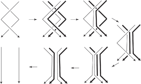
Figure 5.7. A realization of Reidemeister II move using colored moves

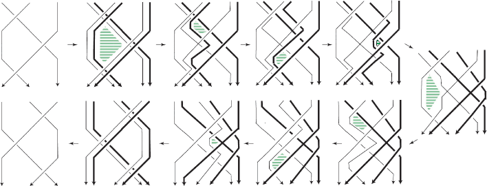
Figure 5.8. A realization of Reidemeister III move using colored moves

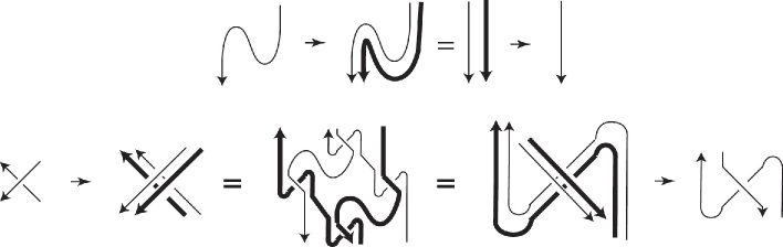
Figure 5.9. Realizations of planar isotopies using colored moves

∎

Note that the diagrammatic transformations in Figure 5.8 induces algebraic equations via the universal invariant $J^{\prime}$, which gives a proof of Proposition 3.5. See the Table 1 for the situation.

Reidemeister III move	$\xrightarrow[]{J^{\prime}}$	quantum Yang-Baxter equation
Colored Pachner $(2,3)$ moves	$\xrightarrow[]{J^{\prime}}$	pentagon relations
Figure 5.8	$\xrightarrow[]{J^{\prime}}$	Proposition 3.5
( Colored $(2,3)$ move $\Rightarrow$ RIII move )		(pentagon relation $\Rightarrow$ quantum Yang-Baxter equation)

Table 1. Correspondence between topological situation and algebraic situation

6. $3$-dimensional descriptions: colored diagrams and colored singular triangulations

In this section we associate a colored tetrahedron to each crossing of a colored diagram $Z$, and define a colored cell complex associated to $Z$. Using a colored cell complex we define a colored singular triangulation of a topological space. As a result, the universal quantum invariant $J^{\prime}$ turns out to be an invariant of colored singular triangulations, where a copy of the $S$-tensor is attached to each colored tetrahedron.

6.1. Colored tetrahedra

Consider a tetrahedron $\Gamma$ in the oriented space $\mathbb{R}^{3}$ with an ordering of its $2$-faces $f_{1},f_{2},f_{3},f_{4}$. We stick $\Gamma$ by two strands going into $\Gamma$ at $f_{1}$ (resp. $f_{3}$) and out of $\Gamma$ at $f_{2}$ (resp. $f_{4}$). Note that there are two types of such tetrahedra up to rotation as in Figure 6.1, where such a tetrahedra is presented by a crossing so that the strand piercing $f_{1}$ and $f_{2}$ is over. We consider two types of strands, depicted by thick and thin strands, and then there are eight types of such tetrahedra, which we call colored tetrahedra, presented by eight types of crossings as in Figure 6.2.

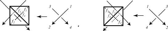
Figure 6.1. Two types of tetrahedra which are sticked by two ordered strands

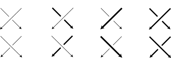
Figure 6.2. Colored tetrahedra

6.2. Colored diagrams and colored cell complexes

We define a colored cell complex $\mathcal{C}(Z)$ associated to a colored diagram $Z$ as follows.

Recall that $Z$ consists of fundamental tangles and symmetries. Let $\{c_{1},\ldots c_{k}\}$ be the set of crossings in $Z$. To each crossing $c_{i}$, associate a colored tetrahedron $\Gamma_{i}$ as in Section 6.1. See Figure 6.3 for an example.

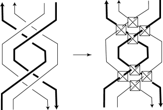
Figure 6.3. How to associate tetrahedra on a colored diagram

We define $\mathcal{C}(Z)$ to be the cell complex obtained from colored tetrahedra $\Gamma_{1},\ldots,\Gamma_{k}$ by gluing them along their $2$-faces as follows.

1. $2$-faces $F$ and $F^{\prime}$ of $\Gamma_{1},\ldots,\Gamma_{k}$ are glued if and only if $F$ and $F^{\prime}$ are adjacent along $Z$.

2. We mark by $*$ the vertex of each $2$-face of $\Gamma_{1},\ldots,\Gamma_{k}$ as in Figure 6.4 depending on the thickness of strands and the order of the faces in a tetrahedron, and glue adjacent faces $F$ and $F^{\prime}$ so that the $*$-marked vertices are attached.

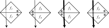
Figure 6.4. How to mark by $*$ a vertex of each triangle

6.3. Colored singular triangulations and colored ideal triangulations

For a space $X$, a singular triangulation (see e.g., [TV92, BB04]) of $X$ consists of a finite index set $I$, a function $d\colon\thinspace I\to\mathbb{N}$, and continuous maps $f_{i}\colon\thinspace\Delta^{d(i)}\to X$ for $i\in I$, where $\Delta^{n}$ is the standard $n$ simplex, such that $(I,d,\{f_{i}\}_{i\in I})$ is a finite cell decomposition of $X$, and for each $i\in I$ and a face $F$ in $\Delta^{d(i)}$, the restriction $f_{i}|_{F}$ is the composition $f_{j}\circ g$ of an affine isomorphism $g\colon\thinspace F\to\Delta^{d(j)}$ and $f_{j}$ for some $j\in I$.

Let $\mathcal{C}(Z)$ be the colored cell complex of a colored diagram $Z$, which we can naturally regard a singular triangulation. Consider

$$X=\mathcal{C}(Z)/(e_{1}=e^{\prime}_{1},\ldots,e_{k}=e^{\prime}_{k},v_{1}=v^{\prime}_{1},\ldots,v_{l}=v^{\prime}_{l})$$

be a singular triangulation obtained from $\mathcal{C}(Z)$ by identifying some pairs of edges $(e_{1},e^{\prime}_{1}),\ldots,(e_{k},e^{\prime}_{k})$, $k\geq 0$, and some pairs of vertices $(v_{1},v^{\prime}_{1}),\ldots,(v_{l},v^{\prime}_{l}),l\geq 0,$ in $\mathcal{C}(Z)$. We call $X$ a colored singular triangulation (coloring) of type $Z$. In particular, if $X$ is an ideal triangulation of some topological space $\tilde{X}$, then we call it a colored ideal triangulation of $\tilde{X}$.

Let $\mathcal{CT}(Z)$ be the set of colored singular triangulations of type $Z$ and set

$$\mathcal{CT}=\bigcup_{Z\in\mathcal{CD}}\mathcal{CT}(Z).$$

Remark 6.1.

In this remark, we assume $3$-manifolds are connected, compact, oriented, and with non-empty boundary.

In [BP14, BB15, BB], Benedetti-Petronio and Baseilhac-Benedetti used so called $\mathcal{N}$-graphs to represent branched ideal triangulations of a $3$-manifolds and dual oriented standard branched spines of them. In this remark we consider abstract $\mathcal{N}$-graphs, i.e., we do not take planar immersions of them.

Let $\mathcal{BTR}$ the set of branched ideal triangulations of $3$-manifolds, $\mathcal{BSP}$ the set of oriented standard branched spines of $3$-manifolds, and $\mathcal{NG}$ the set of $\mathcal{N}$-graphs with the color $0\in\mathbb{Z}/3\mathbb{Z}$ on every edge.

We have the bijections

$$\mathcal{NG}\to\mathcal{BSP},\quad G\mapsto BSP(G),$$

$$\mathcal{NG}\to\mathcal{BTR},\quad G\mapsto BTR(G),$$

where $BSP(G)$ is obtained from $G$ [BB15] so that a $4$-valent vertex encodes a branched tetrahedron, and $BTR(G)$ is the branched ideal triangulations which is the dual of the oriented standard branched spine $BSP(G)$.

Let $\mathcal{CCD}$ be the set of equivalence classes of closed colored diagrams up to planar isotopies and symmetry moves. We have the surjective map

$$p\colon\thinspace\mathcal{CCD}\to\mathcal{NG},\quad Z\mapsto p(Z)$$

where $p(Z)$ is the $\mathcal{N}$-graph obtained from $D$ by reversing the orientation of thick strands.

It is not difficult to check that the branched ideal triangulation $BTR(p(Z))$ is the colored singular triangulation of type $Z$ obtained from $\mathcal{C}(Z)$ by identifying some edges and vertices so that $BSP(p(Z))$ becomes a standard spine, i.e., the complement of the vertices in the singular set of $BSP(p(Z))$ is a union of segments, and the complement of the singular set in $BSP(p(Z))$ is a union of disks. For an example with link complements, see the proof of Proposition 7.1.

6.4. Colored moves and colored singular triangulations

We can translate colored moves on the set $\mathcal{CD}$ of colored diagrams defined in Section 5.2 to moves on the set $\mathcal{CT}$ of colored singular triangulations as follows.

For colored diagrams $Z$ and $Z^{\prime}$, let $X$ and $X^{\prime}$ be colored singular triangulations of types $Z$ and $Z^{\prime}$, respectively. Let

$$\psi\colon\thinspace\mathcal{C}(Z)\to X,\quad\psi^{\prime}\colon\thinspace\mathcal{C}(Z^{\prime})\to X^{\prime},$$

be the projections. We say that $X$ and $X^{\prime}$ are related by a colored Pachner $(2,3)$ move if

1. the colored diagram $Z$ and $Z^{\prime}$ are related by a colored Pachner $(2,3)$ move, and

2. $\psi=\psi^{\prime}$ on the exteriors $\mathcal{C}(Z)\setminus W=\mathcal{C}(Z^{\prime})\setminus W^{\prime}$, where $W$ (resp. $W^{\prime}$) is the subcomplexes of $\mathcal{C}(Z)$ (resp. $\mathcal{C}(Z^{\prime})$) consisting of the three (resp. two) tetrahedra corresponding to the three (resp. two) crossings of $Z$ (resp. $Z^{\prime}$) involved in the colored Pachner $(2,3)$ move.

We define other colored moves on colored singular triangulations similarly.

Then the colored Pachner $(2,3)$ move on $\mathcal{CT}$ turns out to be the Pachner $(2,3)$ move on singular triangulations, defined in Figure 6.5 (a), replacing two tetrahedra sharing one face with three tetrahedra, or its inverse. See Figure 6.6 for an example, where we color over-strands red and under-strands blue so that we can distinguish them in $3$-spaces in the lowest picture.

The colored $(0,2)$ move on $\mathcal{CT}$ turns out to be the $(0,2)$ move on singular triangulations, defined in Figure 6.5 (b), replacing two adjacent $2$-faces with two tetrahedra, or its inverse.

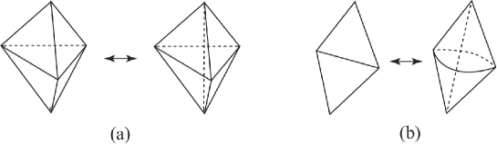
Figure 6.5. (a) The Pachner $(2,3)$ move, (b) The $(0,2)$ move

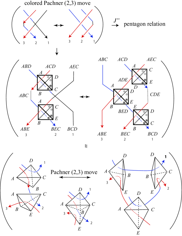
Figure 6.6. A colored Pachner $(2,3)$ move of colored diagrams and a Pachner $(2,3)$ move of colored cell complexes, whose image of $J^{\prime}$ turns out to be the pentagon relation $S_{23}S_{12}=S_{12}S_{13}S_{23}$

Correspondingly to the equivalence relations $\sim_{c}$ and $\sim^{\prime}_{c}$ on $\mathcal{CD}$, we define the equivalence relations $\sim_{ct}$ and $\sim^{\prime}_{ct}$ on $\mathcal{CT}$, i.e., $\sim_{ct}$ is generated by all colored moves, and $\sim^{\prime}_{ct}$ is generated by colored moves except for the moves in Figure 5.6.

Let $\pi\colon\thinspace\mathcal{CT}\to\mathcal{CD}$ be the map such that $\pi(X)=Z$ for $X\in\mathcal{CT}(Z)$.

For $\mu=(\mu_{1},\ldots,\mu_{m}),\nu=(\nu_{1},\ldots,\nu_{m})\in\{\pm\}^{m}$, $m\geq 0$, recall from Sect 5.1 the subset $\mathcal{CD}(\mu;\nu)\subset\mathcal{CD}$. Let $\mathcal{CT}(\mu;\nu)$ be the set of colored singular triangulations of types in $\mathcal{CD}(\mu;\nu)$. Note that $\mathcal{CT}=\bigcup_{\mu,\nu\in\{\pm\}^{m},m\geq 0}\mathcal{CT}(\mu;\nu)$.

Proposition 6.2.

The composition

$$J^{\prime}\circ\pi\colon\thinspace\mathcal{CT}(\mu;\nu)\to\bigotimes_{i\in I_{+}}H(A)_{i}^{\nu_{i}}\bigotimes_{j\in I_{-}}(H(A)^{\mathrm{op}})_{j}^{\nu_{j}}$$

of the restriction of $\pi$ to $\mathcal{CT}(\mu;\nu)$ and the universal quantum invariant $J^{\prime}$ is an invariant under $\sim^{\prime}_{ct}$. If $\gamma^{2}=1$, then $J^{\prime}\circ\pi$ is also an invariant under $\sim_{ct}$.

Proof.

Note that the projection map $\pi$ induces the map

$$\mathcal{CT}/\sim^{\prime}_{ct}\to\mathcal{CD}/\sim^{\prime}_{c}\quad(\text{resp. \ }\mathcal{CT}/\sim_{ct}\to\mathcal{CD}/\sim_{c}),$$

which shows the invariance of $J^{\prime}\circ\pi$ under $\sim^{\prime}_{ct}$ (resp. $\sim_{ct}$ if $\gamma^{2}=1$). ∎

We call $J^{\prime}\circ\pi$ the universal quantum invariant of colored singular triangulations. Note that the invariance of $J^{\prime}\circ\pi$ under colored Pachner $(2,3)$ moves are shown by pentagon relations.

7. Octahedral triangulation of tangle complements

In this section we define ideal triangulations of tangle complements, and construct examples called the octahedral triangulations. We will show that the octahedral triangulation associated to a tangle diagram $D$ naturally admits a structure of a colored ideal triangulation of type $\zeta(D)$.

7.1. Ideal triangulations of tangle complements

Let $M$ be a compact manifold of dimension $n\leq 3$, possibly with non-empty boundary. Let $F$ be an $(n-1)$-submanifold of $\partial M$. Let $F_{1},...,F_{k}$ be the connected components of $F$. Let $M//F$ denote the topological space obtained from $M$ by collapsing each $F_{i}$ into a point. An ideal triangulation of the pair $(M,F)$ is defined to be a singular triangulation of $M//F$ such that each vertex of the singular triangulation is on a point arising from $F$.

Let $D_{n}=[0,1]^{2}\setminus(P_{1}\cup\cdots\cup P_{n})$ be a punctured disk, where $P_{1},\ldots,P_{n}$ are small disks with the centers arranged on the line $[0,1]\times\{1/2\}$ as in Figure 7.1(a). We define the leaves-ideal triangulation $l_{n}$ of $D_{n}$ to be the ideal triangulation of the pair $(D_{n},([0,1]\times\{0,1\})\cup\partial P_{1}\cup\cdots\cup\partial P_{n})$ as in Figure 7.1(b), where we denote by $-\infty,+\infty,p_{1},\ldots,p_{n}$ the vertices corresponding to $[0,1]\times\{0\},[0,1]\times\{1\},\partial P_{1},\ldots,\partial P_{n}$, respectively. Here we formally define $l_{0}$ as a segment having $\{\pm\infty\}$ as its vertices. In particular we call $l_{1}$ a leaf.

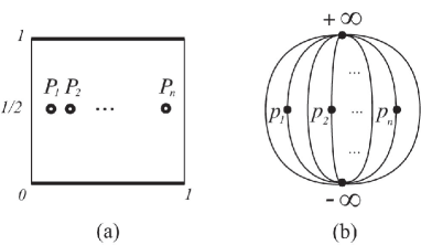
Figure 7.1. (a) A punctured disk and (b) its leaves-ideal triangulation

Let $T=T_{1}\cup\cdots\cup T_{n}$ be an $n$-component tangle. Let $E=\overline{[0,1]^{3}\setminus N(T)}$ be the complement of $T$ in the cube, where $N(T)$ is a tubular neighborhood of $T$ in the cube. Let $F_{T}$ be the intersection $\partial E\cap N(T)$, which consists of annuli and tori. Then an ideal triangulation of the tangle complement $E$ of $T$ in the cube is defined to be an ideal triangulation of $(E,F_{T}\cup F_{z=0}\cup F_{z=1})$, where $F_{z=0}=[0,1]\times[0,1]\times\{0\}$ and $F_{z=1}=[0,1]\times[0,1]\times\{1\}$, such that its restriction to each boundary component $[0,1]\times\{0,1\}\times[0,1]$ is a leaves-ideal triangulation. The vertices corresponding to $F_{z=0}$, and $F_{z=1}$ are denoted by $-\infty$ and $+\infty$, respectively.

7.2. Colored ideal triangulations for octahedral triangulations of tangle complements

A tangle diagram $D$ is called non-splitting if

1. the $4$-regular plane graph giving the diagram $D$ is connected, and

2. there is not a component of $D$ such that crossings along the path of the component are only over-passing or only under-passing.

Let $T$ be a tangle and $D$ its non-splitting diagram which has at least one crossing. We define a cell complex $\mathcal{O}(D)$, which we call the octahedral triangulations associated to $D$, which is an ideal triangulation of the tangle complement $E$. If in addition $D$ is a link diagram, then $\mathcal{O}(D)$ is nothing but the octahedral triangulation studied in e.g., [CKK14, Yok11] in the context of the hyperbolic geometry.

Step 1. Take a colored diagram

Recall from Section 4 the colored diagram $\zeta(D)$ obtained from $D$ by duplicating and thickening the left strands following the orientation.

Step 2. Preparing and placing octahedra

Let $\{c_{1},\ldots c_{k}\}$ be the set of crossings of the diagram $D$. In a neighborhood of $\zeta(c_{i})$, there are four crossings $t_{1}^{i},t_{2}^{i},t_{3}^{i},t_{4}^{i}$ as in Fig 7.2, where $t_{1}^{i}$ is the right crossing when we see strands oriented downwards, and $t_{2}^{i},t_{3}^{i},t_{4}^{i}$ are defined one by one in a counterclockwise order. As in Figure 7.2, for $j=1,2,3,4,$ we associate a tetrahedron $\Lambda_{j}^{i}=n^{i}_{j}\tilde{e}^{i}_{j}\tilde{e}^{\prime i}_{j}s^{i}_{j}$ to each $t_{j}^{i}$. Then we glue the four tetrahedra $\Lambda_{1}^{i},\Lambda_{2}^{i},\Lambda_{3}^{i},\Lambda_{4}^{i}$ together to obtain an octahedron $o_{i}=n^{i}e^{i}_{12}e^{i}_{23}e^{i}_{34}e^{i}_{41}s^{i}$, so that $n^{i}_{j}$, $\tilde{e}^{i}_{j}$, $\tilde{e}^{\prime i}_{j}$, and $s^{i}_{j}$ are going to $n^{i}$, $e^{i}_{j-1,j}$, $e^{i}_{j,j+1}$, and $s^{i}$, respectively, where the index $j$ should be considered modulo $4$. We place $o_{i}$ between the two original strands of $c_{i}$ so that $n^{i}$ and $s^{i}$ are placed on the over-strand and the under-strand, respectively.

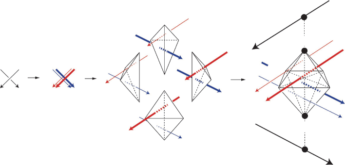
Figure 7.2. Octahedral triangulation around a crossing

Step 3. Gluing octahedra

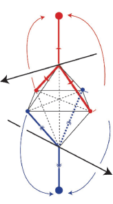
Figure 7.3. How to glue the edges in a octahedron

We glue the octahedra $o_{1},\ldots,o_{k}$ as follows.

For each positive (resp. negative) crossing $c_{i}$, we pull the vertices $e^{i}_{23}$ and $e^{i}_{41}$ (resp. $e^{i}_{12}$ and $e^{i}_{34}$) upwards, put them on $+\infty$, and glue the two edges $n^{i}$-$e^{i}_{23}$ and $n^{i}$-$e_{41}$ (resp. $n^{i}$-$e^{i}_{12}$ and $n^{i}$-$e_{34}$). Similarly, pull the vertices $e^{i}_{12}$ and $e^{i}_{34}$ (resp. $e^{i}_{23}$ and $e^{i}_{41}$) downwards, put them on $-\infty$, and glue the two edges $s^{i}$-$e^{i}_{12}$ and $s^{i}$-$e_{34}$ (resp. $s^{i}$-$e^{i}_{23}$ and $s^{i}$-$e_{41}$), see Figure 7.3. Note that the boundary of the octahedron $o_{i}$ consists of four leaves corresponding to the four edge of $c_{i}$, see Figure 7.4. We glue the octahedra $o_{1},\ldots,o_{k}$ along the pairs of leaves which are adjacent on $D$ so that $\pm\infty$ are attached compatibly. We call the result the octahedral triangulation of the complement of $T$ associated to a diagram $D$, and denote it by $\mathcal{O}(D)$.

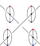
Figure 7.4. Leaves corresponding to the four edges of a crossing

It is not difficult to check that $\mathcal{O}(D)$ is an ideal triangulation of the complement of $T$. Moreover, we have the following.

Proposition 7.1.

The octahedral triangulation $\mathcal{O}(D)$ associated to a tangle diagram $D$ admits a colored ideal triangulation of type $\zeta(D)$.

Proof.

Recall that in Step 2 of the definition of $\mathcal{O}(D)$, we associate an octahedron $o_{i}$ to each crossing $c_{i}$, where the octahedron is obtained from four tetrahedra as in Figure 7.2. Actually we can obtain $o_{i}$ also as the colored cell complex $\mathcal{C}(\zeta(c_{i}))$ as depicted in Figure 7.5. In Step 3, we glued the octahedra and triangles as in Figure 7.6, which follows the gluing rule of the colored tetrahedra and triangles defined in Section 6.2. As the result we have $\mathcal{C}(\zeta(D))$, and finally we identify the edges of each octahedron as in Figure 7.3, which gives $\mathcal{O}(D)$ which is singular triangulation of type $\zeta(D)$. This completes the proof.

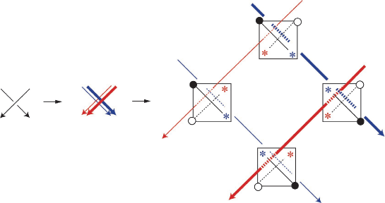
Figure 7.5. The colored ideal triangulation and the octahedron at a crossing of a tangle

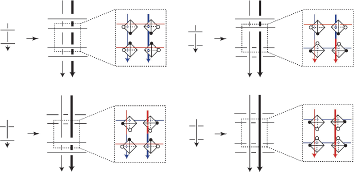
Figure 7.6. How we glued the octahedra in the octahedral triangulations, where the black dots are attached to $+\infty$ and the white dots are attached to $-\infty$.

∎

Remark 7.2.

A tangle complement could admit more than one colored ideal triangulations up to the equivalence relation $\sim^{\prime}_{ct}$, and the universal quantum invariant $J^{\prime}$ could give different values on them. We expect that the universal quantum invariant is an invariant of pairs of $3$-manifolds and some geometrical inputs obtained from the color, which we will study in [KST].

References

- [BS93] S. Baaj, G. Skandalis, Unitaires multiplicatifs et dualité pour les produits croisés de -algèbres. Ann. Sci. École Norm. Sup. (4) 26 (1993), no. 4, 425–488.
- [BB04] S. Baseilhac, R. Benedetti, Quantum hyperbolic invariants of 3-manifolds with -characters. Topology 43 (2004), no. 6, 1373–1423.
- [BB05] S. Baseilhac, R. Benedetti, Classical and quantum dilogarithmic invariants of flat -bundles over 3-manifolds. Geom. Topol. 9 (2005), 493–569 (electronic).
- [BB07] S. Baseilhac, R. Benedetti, Quantum hyperbolic geometry. Algebr. Geom. Topol. 7 (2007), 845–917.
- [BB11] S. Baseilhac, R. Benedetti, The Kashaev and quantum hyperbolic link invariants. J. Gökova Geom. Topol. GGT 5 (2011), 31–85.
- [BB15] S. Baseilhac, R. Benedetti, Analytic families of quantum hyperbolic invariants. (English summary) Algebr. Geom. Topol. 15 (2015), no. 4, 1983–2063.
- [BB] S. Baseilhac, R. Benedetti, Non ambiguous structures on 3-manifolds and quantum symmetry defects, to appear in Quantum Topology.
- [BP97] R. Benedetti, C. Petronio, Branched standard spines of 3-manifolds. Lecture Notes in Mathematics, 1653. Springer-Verlag, Berlin, 1997.
- [BP14] R. Benedetti, C. Petronio, Spin structures on 3-manifolds via arbitrary triangulations. (English summary) Algebr. Geom. Topol. 14 (2014), no. 2, 1005–1054.
- [CKK14] J. Cho H. Kim, S. Kim, Optimistic limits of Kashaev invariants and complex volumes of hyperbolic links. (English summary) J. Knot Theory Ramifications 23 (2014), no. 9, 1450049, 32 pp.
- [Dri87] V. G. Drinfeld, Quantum groups. Proceedings of the International Congress of Mathematicians, Vol. 1, 2 (Berkeley, Calif., 1986), 798–820, Amer. Math. Soc., Providence, RI, 1987.
- [FK94] L. D. Faddeev, R. M. Kashaev, Quantum dilogarithm. Modern Phys. Lett. A 9 (1994), no. 5, 427–434.
- [Hab06] K. Habiro, Bottom tangles and universal invariants. Algebr. Geom. Topol. 6 (2006), 1113–1214.
- [HI14] K. Hikami, R. Inoue, Braiding operator via quantum cluster algebra. (English summary) J. Phys. A 47 (2014), no. 47, 474006, 21 pp.
- [HI15] K. Hikami, R. Inoue, Braids, complex volume and cluster algebras. (English summary) Algebr. Geom. Topol. 15 (2015), no. 4, 2175–2194.
- [KST] A. Kato, S. Suzuki, Y. Terashima, in preparation.
- [KR01] L. Kauffman, D. E. Radford, Oriented quantum algebras, categories and invariants of knots and links. J. Knot Theory Ramifications 10 (2001), no. 7, 1047–1084.
- [Kap98] M. Kapranov, Heisenberg doubles and derived categories. J. Algebra 202 (1998), no. 2, 712–744.
- [Kash94] R. M. Kashaev, Quantum dilogarithm as a 6j-symbol. Modern Phys. Lett. A 9 (1994), no. 40, 3757–3768.
- [Kash95] R. M. Kashaev, A link invariant from quantum dilogarithm. (English summary) Modern Phys. Lett. A 10 (1995), no. 19, 1409–1418.
- [Kash97] R. M. Kashaev, The Heisenberg double and the pentagon relation. (English summary) Algebra i Analiz 8 (1996), no. 4, 63–74; translation in St. Petersburg Math. J. 8 (1997), no. 4, 585–592.
- [Kash97’] R. M. Kashaev, The hyperbolic volume of knots from the quantum dilogarithm. Lett. Math. Phys. 39 (1997), no. 3, 269–275.
- [Kash98] R. M. Kashaev, An invariant of triangulated links from a quantum dilogarithm. (Russian) Zap. Nauchn. Sem. S.-Peterburg. Otdel. Mat. Inst. Steklov. (POMI) 224 (1995), Voprosy Kvant. Teor. Polya i Statist. Fiz. 13, 208–214, 339; translation in J. Math. Sci. (New York) 88 (1998), no. 2, 244–248.
- [Kash01] R. M. Kashaev, On the spectrum of Dehn twists in quantum Teichmüller theory. (English summary) Physics and combinatorics, 2000 (Nagoya), 63–81, World Sci. Publ., River Edge, NJ, 2001.
- [Kass95] C. Kassel, Quantum groups. Graduate Texts in Mathematics, 155, Springer-Verlag, New York, 1995.
- [Law90] R. J. Lawrence, A universal link invariant. The interface of mathematics and particle physics (Oxford, 1988), 151–156, Inst. Math. Appl. Conf. Ser. New Ser., 24, Oxford Univ. Press, New York, 1990.
- [Law89] R. J. Lawrence, A universal link invariant using quantum groups. Differential geometric methods in theoretical physics (Chester, 1988), 55–63, World Sci. Publ., Teaneck, NJ, 1989.
- [Lu94] J.-H. Lu, On the Drinfel’d double and the Heisenberg double of a Hopf algebra. Duke Math. J. 74 (1994), no. 3, 763–776.
- [Maj98] S. Majid, Quantum double for quasi-Hopf algebras. Lett. Math. Phys. 45 (1998), no. 1, 1–9.
- [Maj99] S. Majid, Double-bosonization of braided groups and the construction of Uq(g). Math. Proc. Cambridge Philos. Soc. 125 (1999), no. 1, 151–192.
- [MM01] H. Murakami, J. Murakami, The colored Jones polynomials and the simplicial volume of a knot. Acta Math. 186 (2001), no. 1, 85–104.
- [Oht93] T. Ohtsuki, Colored ribbon Hopf algebras and universal invariants of framed links. J. Knot Theory Ramifications 2 (1993), no. 2, 211–232.
- [Oc94] A. Ocneanu, Chirality for operator algebras, in ”Subfactors”, ed. by H. Araki, et al., World
- [RT90] N. Y. Reshetikhin, V. G. Turaev, Ribbon graphs and their invariants derived from quantum groups. Comm. Math. Phys. 127 (1990), no. 1, 1–26.
- [Sem92] M. A. Semenov-Tian-Shansky, Poisson Lie groups, quantum duality principle, and the quantum double. Mathematical aspects of conformal and topological field theories and quantum groups (South Hadley, MA, 1992), 219–248, Contemp. Math., 175, Amer. Math. Soc., Providence, RI, 1994.
- [Suz12] S. Suzuki, On the universal invariant of boundary bottom tangles, Algebr. Geom. Topol. 12 (2012), 997–1057.
- [TV92] V.G. Turaev, O.Y. Viro, State-sum invariants of 3-manifolds and quantum 6j-symbols, Topology, 31 (1992), pp. 865–902.
- [Yok11] Y. Yokota. On the complex volume of hyperbolic knots. J. Knot Theory Ramifications, 20 (7):955–976, 2011.
- [We05] J. Weeks. Computation of hyperbolic structures in knot theory. In Handbook of knot theory, pages 461–480. Elsevier B. V., Amsterdam, 2005.