Change point estimation based on Wilcoxon tests in the presence of long-range dependence

Abstract

We consider an estimator for the location of a shift in the mean of long-range dependent sequences. The estimation is based on the two-sample Wilcoxon statistic. Consistency and the rate of convergence for the estimated change point are established. In the case of a constant shift height, the $1/n$ convergence rate (with $n$ denoting the number of observations), which is typical under the assumption of independent observations, is also achieved for long memory sequences. It is proved that if the change point height decreases to $0$ with a certain rate, the suitably standardized estimator converges in distribution to a functional of a fractional Brownian motion. The estimator is tested on two well-known data sets. Finite sample behaviors are investigated in a Monte Carlo simulation study.

t2Research supported by the German National Academic Foundation and Collaborative Research Center SFB 823 Statistical modelling of nonlinear dynamic processes.

1 Introduction

Suppose that the observations $X_{1},\ldots,X_{n}$ are generated by a stochastic process $\left(X_{i}\right)_{i\geq 1}$

$$X_{i}=\mu_{i}+Y_{i},$$

where $(\mu_{i})_{i\geq 1}$ are unknown constants and where $(Y_{i})_{i\geq 1}$ is a stationary, long-range dependent (LRD, in short) process with mean zero. A stationary process $(Y_{i})_{i\geq 1}$ is called “long-range dependent” if its autocovariance function $\rho$, $\rho(k):={\operatorname{Cov}}(Y_{1},Y_{k+1})$, satisfies

$$\rho(k)\sim k^{-D}L(k),\ \text{as }k\rightarrow\infty,$$ (1)

where $0<D<1$ (referred to as long-range dependence (LRD) parameter) and where $L$ is a slowly varying function.

Furthermore, we assume that there is a change point in the mean of the observations, that is

$$\mu_{i}=\begin{cases}\mu,&\text{for}\ i=1,\ldots,k_{0},\\ \mu+h_{n},&\text{for}\ i=k_{0}+1,\ldots,n,\end{cases}$$

where $k_{0}=\lfloor n\tau\rfloor$ denotes the change point location and $h_{n}$ is the height of the level-shift.

In the following we differentiate between fixed and local changes. Under fixed changes we assume that $h_{n}=h$ for some $h\neq 0$. Local changes are characterized by a sequence $h_{n}$, $n\in\mathbb{N}$, with $h_{n}\longrightarrow 0$ as $n\longrightarrow\infty$; in other words, in a model where the height of the jump decreases with increasing sample size $n$.

In order to test the hypothesis

$$H:\mu_{1}=\ldots=\mu_{n}$$

against the alternative

$$A:\mu_{1}=\ldots=\mu_{k}\neq\mu_{k+1}=\ldots=\mu_{n}\ \text{for some $k\in\left\{1,\ldots,n-1\right\}$}$$

the Wilcoxon change point test can be applied. It rejects the hypothesis for large values of the Wilcoxon test statistic defined by

$$W_{n}:=\max\limits_{1\leq k\leq n-1}\left|W_{k,n}\right|,\ \text{where}\ W_{k,n}:=\sum\limits_{i=1}^{k}\sum\limits_{j=k+1}^{n}\left(1_{\left\{X_{i}\leq X_{j}\right\}}-\frac{1}{2}\right)$$

(see Dehling, Rooch and Taqqu (2013a)). Under the assumption that there is a change point in the mean in $k_{0}$ we expect the absolute value of $W_{k_{0},n}$ to exceed the absolute value of $W_{l,n}$ for any $l\neq k_{0}$. Therefore, it seems natural to define an estimator of $k_{0}$ by

$$\hat{k}_{W}=\hat{k}_{W}(n):=\min\left\{k:\left|W_{k,n}\right|=\max\limits_{1\leq i\leq n-1}\left|W_{i,n}\right|\right\}.$$

Preceding papers that address the problem of estimating change point locations in dependent observations $X_{1},\ldots,X_{n}$ with a shift in mean often refer to a family of estimators based on the CUSUM change point test statistics $C_{n}(\gamma):=\max_{1\leq k\leq n-1}|C_{k,n}(\gamma)|$, where

$$C_{k,n}(\gamma):=\left(\frac{k(n-k)}{n}\right)^{1-\gamma}\left(\frac{1}{k}\sum\limits_{i=1}^{k}X_{i}-\frac{1}{n-k}\sum\limits_{i=k+1}^{n}X_{i}\right)$$

with parameter $0\leq\gamma<1$. The corresponding change point estimator is defined by

$$\hat{k}_{C,\gamma}=\hat{k}_{C,\gamma}(n):=\min\left\{k:\left|C_{k,n}(\gamma)\right|=\max\limits_{1\leq i\leq n-1}\left|C_{i,n}(\gamma)\right|\right\}.$$ (2)

For long-range dependent Gaussian processes Horváth and Kokoszka (1997) derive the asymptotic distribution of the estimator $\hat{k}_{C,\gamma}$ under the assumption of a decreasing jump height $h_{n}$, i.e. under the assumption that $h_{n}$ approaches $0$ as the sample size $n$ increases. Under non-restrictive constraints on the dependence structure of the data-generating process (including long-range dependent time series) Kokoszka and Leipus (1998) prove consistency of $\hat{k}_{C,\gamma}$ under the assumption of fixed as well as decreasing jump heights. Furthermore, they establish the convergence rate of the change point estimator as a function of the intensity of dependence in the data if the jump height is constant. Ben Hariz and Wylie (2005) show that under a similar assumption on the decay of the autocovariances the convergence rate that is achieved in the case of independent observations can be obtained for short- and long-range dependent data, as well. Furthermore, it is shown in their paper that for a decreasing jump height the convergence rate derived by Horváth and Kokoszka (1997) under the assumption of gaussianity can also be established under more general assumptions on the data-generating sequences.

Bai (1994) establishes an estimator for the location of a shift in the mean by the method of least squares. He proves consistency, determines the rate of convergence of the change point estimator and derives its asymptotic distribution. These results are shown to hold for weakly dependent observations that satisfy a linear model and cover, for example, ARMA($p$, $q$)-processes. Bai extended these results to the estimation of the location of a parameter change in multiple regression models that also allow for lagged dependent variables and trending regressors (see Bai (1997)). A generalization of these results to possibly long-range dependent data-generating processes (including fractionally integrated processes) is given in Kuan and Hsu (1998) and Lavielle and Moulines (2000). Under the assumption of independent data Darkhovskh (1976) establishes an estimator for the location of a change in distribution based on the two-sample Mann-Whitney test statistic. He obtains a convergence rate that has order $\frac{1}{n}$, where $n$ is the number of observations. Allowing for strong dependence in the data Giraitis, Leipus and Surgailis (1996) consider Kolmogorov-Smirnov and Cramér-von-Mises-type test statistics for the detection of a change in the marginal distribution of the random variables that underlie the observed data. Consistency of the corresponding change point estimators is proved under the assumption that the jump height approaches $0$. A change point estimator based on a self-normalized CUSUM test statistic has been applied in Shao (2011) to real data sets. Although Shao assumes validity of using the estimator, the article does not cover a formal proof of consistency. Furthermore, it has been noted by Shao and Zhang (2010) that even under the assumption of short-range dependence it seems difficult to obtain the asymptotic distribution of the estimate.

In this paper we shortly address the issue of estimating the change point location on the basis of the self-normalized Wilcoxon test statistic proposed in Betken (2016).

In order to construct the self-normalized Wilcoxon test statistic, we have to consider the ranks $R_{i}$, $i=1,\ldots,n$, of the observations $X_{1},\ldots,X_{n}$. These are defined by $R_{i}:={\operatorname{rank}}(X_{i})=\sum_{j=1}^{n}1_{\{X_{j}\leq X_{i}\}}$ for $i=1,\ldots,n$. The self-normalized two-sample test statistic is defined by

$$SW_{k,n}=\frac{\sum_{i=1}^{k}R_{i}-\frac{k}{n}\sum_{i=1}^{n}R_{i}}{\bigg{\{}\frac{1}{n}\sum_{t=1}^{k}S_{t}^{2}(1,k)+\frac{1}{n}\sum_{t=k+1}^{n}S_{t}^{2}(k+1,n)\bigg{\}}^{1/2}},$$

where

$$S_{t}(j,k):=\sum\limits_{h=j}^{t}\left(R_{h}-\bar{R}_{j,k}\right)\ \ \text{with }\bar{R}_{j,k}:=\frac{1}{k-j+1}\sum\limits_{t=j}^{k}R_{t}.$$

The self-normalized Wilcoxon change point test for the test problem $(H,A)$ rejects the hypothesis for large values of $T_{n}(\tau_{1},\tau_{2})=\max_{k\in\left\{\lfloor n\tau_{1}\rfloor,\ldots,\lfloor n\tau_{2}\rfloor\right\}}\left|SW_{k,n}\right|$, where $0<\tau_{1}<\tau_{2}<1$. Note that the proportion of the data that is included in the calculation of the supremum is restricted by $\tau_{1}$ and $\tau_{2}$. A common choice for these parameters is $\tau_{1}=1-\tau_{2}=0.15$; see Andrews (1993).

A natural change point estimator that results from the self-normalized Wilcoxon test statistic is

$$\hat{k}_{SW}=\hat{k}_{SW}(n):=\min\left\{k:\left|SW_{k,n}\right|=\max\limits_{\lfloor n\tau_{1}\rfloor\leq i\leq\lfloor n\tau_{2}\rfloor}\left|SW_{i,n}\right|\right\}.$$

We will prove consistency of the estimator $\hat{k}_{SW}$ under fixed changes and under local changes whose height converges to $0$ with a rate depending on the intensity of dependence in the data. Nonetheless, the main aim of this paper is to characterize the asymptotic behavior of the change point estimator $\hat{k}_{W}$. In Section 2 we establish consistency of $\hat{k}_{W}$ and $\hat{k}_{SW}$, derive the optimal convergence rate of $\hat{k}_{W}$ and finally consider its asymptotic distribution. Applications to two well-known data sets can be found in Section 3. The finite sample properties of the estimators are investigated by simulations in Section 4. Proofs of the theoretical results are given in Section 5.

2 Main Results

Recall that for fixed $x$, $x\in\mathbb{R}$, the Hermite expansion of $1_{\left\{G(\xi_{i})\leq x\right\}}-F(x)$ is given by

$$1_{\left\{G(\xi_{i})\leq x\right\}}-F(x)=\sum\limits_{q=1}^{\infty}\frac{J_{q}(x)}{q!}H_{q}(\xi_{i}),$$

where $H_{q}$ denotes the $q$-th order Hermite polynomial and where

$$J_{q}(x)={\operatorname{E}}\left(1_{\left\{G(\xi_{i})\leq x\right\}}H_{q}(\xi_{i})\right).$$

Assumption 1.

Let $Y_{i}=G(\xi_{i})$, where $\left(\xi_{i}\right)_{i\geq 1}$ is a stationary, long-range dependent Gaussian process with mean $0$, variance $1$ and LRD parameter $D$. We assume that $0<D<\frac{1}{r}$, where $r$ denotes the Hermite rank of the class of functions $1_{\left\{G(\xi_{i})\leq x\right\}}-F(x)$, $x\in\mathbb{R}$, defined by

$$r:=\min\left\{q\geq 1:J_{q}(x)\neq 0\ \text{for some}\ x\in\mathbb{R}\right\}.$$

Moreover, we assume that $G:\mathbb{R}\longrightarrow\mathbb{R}$ is a measurable function and that $\left(Y_{i}\right)_{i\geq 1}$ has a continuous distribution function $F$.

Let

$$g_{D,r}(t):=t^{\frac{rD}{2}}L^{-\frac{r}{2}}(t)$$

and define

$$d_{n,r}:=\frac{n}{g_{D,r}(n)}c_{r},\ \text{where}\ c_{r}:=\sqrt{\frac{2r!}{(1-Dr)(2-Dr)}}.$$

Since $g_{D,r}$ is a regularly varying function, there exists a function $g_{D,r}^{-}$ such that

$$g_{D,r}(g_{D,r}^{-}(t))\sim g_{D,r}^{-}(g_{D,r}(t))\sim t,\text{ as $t\rightarrow\infty$,}$$

(see Theorem 1.5.12 in Bingham, Goldie and Teugels (1987)). We refer to $g_{D,r}^{-}$ as the asymptotic inverse of $g_{D,r}$.

The following result states that $\frac{\hat{k}_{W}}{n}$ and $\frac{\hat{k}_{SW}}{n}$ are consistent estimators for the change point location under fixed as well as certain local changes.

Proposition 1.

Suppose that Assumption 1 holds. Under fixed changes, $\frac{\hat{k}_{W}}{n}$ and $\frac{\hat{k}_{SW}}{n}$ are consistent estimators for the change point location. The estimators are also consistent under local changes if $h_{n}^{-1}=o\left(\frac{n}{d_{n,r}}\right)$ and if $F$ has a bounded density $f$. In other words, we have

$$\frac{\hat{k}_{W}}{n}\overset{P}{\longrightarrow}\tau,\qquad\frac{\hat{k}_{SW}}{n}\overset{P}{\longrightarrow}\tau$$

in both situations. Furthermore, it follows that the Wilcoxon test is consistent under these assumptions (in the sense that $\frac{1}{nd_{n,r}}\max_{1\leq k\leq n-1}|W_{k,n}|\overset{P}{\longrightarrow}\infty$).

The following theorem establishes a convergence rate for the change point estimator $\hat{k}_{W}$. Note that only under local changes the convergence rate depends on the intensity of dependence in the data.

Theorem 1.

Suppose that Assumption 1 holds and let $m_{n}:=g_{D,r}^{-}(h_{n}^{-1})$. Then, we have

$$\left|\hat{k}_{W}-k_{0}\right|=\mathcal{O}_{P}(m_{n})$$

if either

• $h_{n}=h$ with $h\neq 0$

or

• $\lim_{n\rightarrow\infty}h_{n}=0$ with $h_{n}^{-1}=o\left(\frac{n}{d_{n,r}}\right)$ and $F$ has a bounded density $f$.

Remark 1.

1. Under fixed changes $m_{n}$ is constant. As a consequence, $|\hat{k}_{W}-k_{0}|=\mathcal{O}_{P}(1)$. This result corresponds to the convergence rates obtained by Ben Hariz and Wylie (2005) for the CUSUM-test based change point estimator and by Lavielle and Moulines (2000) for the least-squares estimate of the change point location. Surprisingly, in this case the rate of convergence is independent of the intensity of dependence in the data characterized by the value of the LRD parameter $D$. An explanation for this phenomenon might be the occurrence of two opposing effects: increasing values of the LRD parameter $D$ go along with a slower convergence of the test statistic $W_{k,n}$ (making estimation more difficult), but a more regular behavior of the random component (making estimation easier) (see Ben Hariz and Wylie (2005)).

2. Note that if $h_{n}^{-1}=o\left(\frac{n}{d_{n,r}}\right)$ and $m_{n}=g_{D,r}^{-}(h_{n}^{-1})$, it holds that

   • $m_{n}\longrightarrow\infty$,

   • $\frac{m_{n}}{n}\longrightarrow 0$,

   • $\frac{d_{m_{n},r}}{m_{n}}\sim h_{n}$,

   as $n\longrightarrow\infty$.

Based on the previous results it is possible to derive the asymptotic distribution of the change point estimator $\hat{k}_{W}$:

Theorem 2.

Suppose that Assumption 1 holds with $r=1$ and assume that $F$ has a bounded density $f$. Let $m_{n}:=g_{D,1}^{-}(h_{n}^{-1})$, let $B_{H}$ denote a fractional Brownian motion process and define $h(s;\tau)$ by

$$h(s;\tau)=\begin{cases}s(1-\tau)\int f^{2}(x)dx&\text{if $s\leq 0$}\\ -s\tau\int f^{2}(x)dx&\text{if $s>0$}\end{cases}.$$

. If $h_{n}^{-1}=o\left(\frac{n}{d_{n,1}}\right)$, then, for all $M>0$,

$$\frac{1}{e_{n}}\left(W_{k_{0}+\lfloor m_{n}s\rfloor,n}^{2}-W_{k_{0},n}^{2}\right),\ -M\leq s\leq M,$$

with $e_{n}=n^{3}h_{n}d_{m_{n},1}$, converges in distribution to

$$2\tau(1-\tau)\int f^{2}(x)dx\left({\operatorname{sign}}(s)B_{H}(s)\int J_{1}(x)dF(x)+h(s;\tau)\right),\ -M\leq s\leq M,$$

in the Skorohod space $D\left[-M,M\right]$. Furthermore, it follows that $m_{n}^{-1}(\hat{k}_{W}-k_{0})$ converges in distribution to

$${\operatorname{argmax}}_{-\infty<s<\infty}\left({\operatorname{sign}}(s)B_{H}(s)\int J_{1}(x)dF(x)+h(s;\tau)\right).$$ (3)

Remark 2.

1. Under local changes the assumption on $h_{n}$ is equivalent to Assumption C.5 (i) in Horváth and Kokoszka (1997). Moreover, the limit distribution (3) closely resembles the limit distribution of the CUSUM-based change point estimator considered in that paper.

2. The proof of Theorem 2 is mainly based on the empirical process non-central limit theorem for subordinated Gaussian sequences in Dehling and Taqqu (1989). The sequential empirical process has also been studied by many other authors in the context of different models. See, among many others, the following: Müller (1970) and Kiefer (1972) for independent and identically distributed data, Berkes and Philipp (1977) and Philipp and Pinzur (1980) for strongly mixing processes, Berkes, Hörmann and Schauer (2009) for S-mixing processes, Giraitis and Surgailis (1999) for long memory linear (or moving average) processes, Dehling, Durieu and Tusche (2014) for multiple mixing processes. Presumably, in these situations the asymptotic distribution of $\hat{k}_{W}$ can be derived by the same argument as in the proof of Theorem 2 for subordinated Gaussian processes. In particular, Theorem 1 in Giraitis and Surgailis (1999) can be considered as a generalization of Theorem 1.1 in Dehling and Taqqu (1989), i.e. with an appropriate normalization the change point estimator $\hat{k}_{W}$, computed with respect to long-range dependent linear processes as defined in Giraitis and Surgailis (1999), should converge in distribution to a limit that corresponds to (3) (up to multiplicative constants).

3 Applications

We consider two well-known data sets which have been analyzed before. We compute the estimator $\hat{k}_{W}$ based on the given observations and put our results into context with the findings and conclusions of other authors.

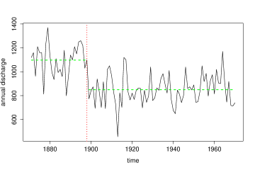
Figure 1: Measurements of the annual discharge of the river Nile at Aswan in $10^{8}m^{3}$ for the years 1871-1970. The dotted line indicates the potential change point estimated by $\hat{k}_{\text{W}}$; the dashed lines designate the sample means for the pre-break and post-break samples.

The plot in Figure 1 depicts the annual volume of discharge from the Nile river at Aswan in $10^{8}m^{3}$ for the years 1871 to 1970. The data set is included in any standard distribution of R. Amongst others, Cobb (1978), Macneill, Tang and Jandhyala (1991), Wu and Zhao (2007), Shao (2011) and Betken and Wendler (2015) provide statistically significant evidence for a decrease of the Nile’s annual discharge towards the end of the 19th century.

The construction of the Aswan Low Dam between 1898 and 1902 serves as a popular explanation for an abrupt change in the data around the turn of the century. Yet, Cobb gave another explanation for the decrease in water volume by citing rainfall records which suggest a decline of tropical rainfall at that time. In fact, an application of the change point estimator $\hat{k}_{W}$ identifies a change in 1898. This result seems to be in good accordance with the estimated change point locations suggested by other authors: Cobb’s analysis of the Nile data leads to the conjecture of a significant decrease in discharge volume in 1898. Moreover, computation of the CUSUM-based change point estimator $\hat{k}_{C,0}$ considered in Horváth and Kokoszka (1997) indicates a change in 1898. Balke (1993) and Wu and Zhao (2007) suggest that the change occurred in 1899.

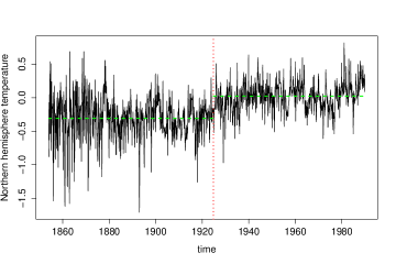
Figure 2: Monthly temperature of the Northern hemisphere for the years 1854-1989 from the data base held at the Climate Research Unit of the University of East Anglia, Norwich, England. The temperature anomalies (in degrees C) are calculated with respect to the reference period 1950-1979. The dotted line indicates the location of the potential change point; the dashed lines designate the sample means for the pre-break and post-break samples.

The second data set consists of the seasonally adjusted monthly deviations of the temperature (degrees C) for the Northern hemisphere during the years 1854 to 1989 from the monthly averages over the period 1950 to 1979. The data has been taken from the longmemo package in R. It results from spatial averaging of temperatures measured over land and sea. In view of the plot in Figure 2 it seems natural to assume that the data generating process is non-stationary. Previous analysis of this data offers different explanations for the irregular behavior of the time series. Deo and Hurvich (1998) fitted a linear trend to the data, thereby providing statistical evidence for global warming during the last decades. However, the consideration of a more general stochastic model by the assumption of so-called semiparametric fractional autoregressive (SEMIFAR) processes in Beran and Feng (2002) does not confirm the conjecture of a trend-like behavior. Neither does the investigation of the global temperature data in Wang (2007) support the hypothesis of an increasing trend. It is pointed out by Wang that the trend-like behavior of the Northern hemisphere temperature data may have been generated by stationary long-range dependent processes. Yet, it is shown in Shao (2011) and also in Betken and Wendler (2015) that under model assumptions that include long-range dependence an application of change point tests leads to a rejection of the hypothesis that the time series is stationary. According to Shao (2011) an estimation based on a self-normalized CUSUM test statistic suggests a change around October 1924. Computation of the change point estimator $\hat{k}_{W}$ corresponds to a change point located around June 1924. The same change point location results from an application of the previously mentioned estimator $\hat{k}_{C,0}$ considered in Horváth and Kokoszka (1997). In this regard estimation by $\hat{k}_{W}$ seems to be in good accordance with the results of alternative change point estimators.

4 Simulations

We will now investigate the finite sample performance of the change point estimator $\hat{k}_{W}$ and compare it to corresponding simulation results for the estimators $\hat{k}_{SW}$ (based on the self-normalized Wilcoxon test statistic) and $\hat{k}_{\text{C},0}$ (based on the CUSUM test statistic with parameter $\gamma=0$) . For this purpose, we consider two different scenarios:

1. Normal margins: We generate fractional Gaussian noise time series $(\xi_{i})_{i\geq 1}$ and choose $G(t)=t$ in Assumption 1. As a result, the simulated observations $\left(Y_{i}\right)_{i\geq 1}$ are Gaussian with autocovariance function $\rho$ satisfying

   $$\rho(k)\sim\left(1-\frac{D}{2}\right)\left(1-D\right)k^{-D}.$$

   Note that in this case the Hermite coefficient $J_{1}(x)$ is not equal to $0$ for all $x\in\mathbb{R}$ (see Dehling, Rooch and Taqqu (2013a)) so that $m=1$, where $m$ denotes the Hermite rank of $1_{\left\{G(\xi_{i})\leq x\right\}}-F(x),x\in\mathbb{R}$. Therefore, Assumption 1 holds for all values of $D\in\left(0,1\right)$.

2. Pareto margins: In order to get standardized Pareto-distributed data which has a representation as a functional of a Gaussian process, we consider the transformation

   $$G(t)=\left(\frac{\beta k^{2}}{(\beta-1)^{2}(\beta-2)}\right)^{-\frac{1}{2}}\left(k(\Phi(t))^{-\frac{1}{\beta}}-\frac{\beta k}{\beta-1}\right)$$

   with parameters $k,\beta>0$ and with $\Phi$ denoting the standard normal distribution function. Since $G$ is a strictly decreasing function, it follows by Theorem 2 in Dehling, Rooch and Taqqu (2013a) that the Hermite rank of $1_{\left\{G(\xi_{i})\leq x\right\}}-F(x),x\in\mathbb{R}$, is $m=1$ so that Assumption 1 holds for all values of $D\in\left(0,1\right)$.

To analyze the behavior of the estimators we simulated $500$ time series of length $600$ and added a level shift of height $h$ after a proportion $\tau$ of the data. We have done so for several choices of $h$ and $\tau$. The descriptive statistics, i.e. mean, sample standard deviation (S.D.) and quartiles, are reported in Tables 1, 2, and 3 for the three change point estimators $\hat{k}_{W}$, $\hat{k}_{SW}$ and $\hat{k}_{C,0}$.

The following observations, made on the basis of Tables 1, 2, and 3, correspond to the expected behavior of consistent change point estimators:

• Bias and variance of the estimated change point location decrease when the height of the level shift increases.

• Estimation of the time of change is more accurate for breakpoints located in the middle of the sample than estimation of change point locations that lie close to the boundary of the testing region.

• High values of $H$ go along with an increase of bias and variance. This seems natural since when there is very strong dependence, i.e. $H$ is large, the variance of the series increases, so that it becomes harder to accurately estimate the location of a level shift.

A comparison of the descriptive statistics of the estimator $\hat{k}_{W}$ (based on the Wilcoxon statistic) and $\hat{k}_{SW}$ (based on the self-normalized Wilcoxon statistic) shows that:

• In most cases the estimator $\hat{k}_{SW}$ has a smaller bias, especially for an early change point location. Nevertheless, the difference between the biases of $\hat{k}_{SW}$ and $\hat{k}_{W}$ is not big.

• In general the sample standard deviation of $\hat{k}_{W}$ is smaller than that of $\hat{k}_{SW}$. Indeed, it is only slightly better for $\tau=0.25$, but there is a clear difference for $\tau=0.5$.

All in all, our simulations do not give rise to choosing $\hat{k}_{SW}$ over $\hat{k}_{W}$. In particular, better standard deviations of $\hat{k}_{W}$ compensate for smaller biases of $\hat{k}_{SW}$.

Comparing the finite sample performance of $\hat{k}_{W}$ and the CUSUM-based change point estimator $\hat{k}_{C,0}$ we make the following observations:

• For fractional Gaussian noise time series bias and variance of $\hat{k}_{C,0}$ tend to be slightly better, at least when $\tau=0.25$ and especially for relatively high level shifts. Nonetheless, the deviations are in most cases negligible.

• If the change happens in the middle of a sample with normal margins, bias and variance of $\hat{k}_{W}$ tend to be smaller, especially for relatively high level shifts. Again, in most cases the deviations are negligible.

• For Pareto($3$, $1$) time series $\hat{k}_{W}$ clearly outperforms $\hat{k}_{C,0}$ by yielding smaller biases and decisively smaller variances for almost every combination of parameters that has been considered. The performance of the estimator $\hat{k}_{C,0}$ surpasses the performance of $\hat{k}_{W}$ only for high values of the jump height $h$.

It is well-known that the Wilcoxon change point test is more robust against outliers in data sets than the CUSUM-like change point tests, i.e. the Wilcoxon test outperforms CUSUM-like tests if heavy-tailed time series are considered. Our simulations confirm that this observation is also reflected by the finite sample behavior of the corresponding change point estimators.

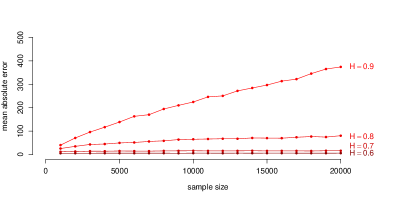
Figure 3: The MAE of $\hat{k}_{W}$ for different values of $H$.

As noted in Remark 1, $\hat{k}_{W}-k_{0}=\mathcal{O}_{P}(1)$ under the assumption of a constant change point height $h$. This observation is illustrated by simulations of the mean absolute error

$$\text{MAE}=\frac{1}{m}\sum\limits_{i=1}^{m}\left|\hat{k}_{W,i}-k_{0}\right|,$$

where $\hat{k}_{W,i}$, $i=1,\ldots,m$, denote the estimates for $k_{0}$, computed on the basis of $m=5000$ different sequences of fractional Gaussian noise time series.

Figure 3 depicts a plot of MAE against the sample size $n$ with $n$ varying between $1000$ and $20000$.

Since $\hat{k}_{W}-k_{0}=\mathcal{O}_{P}(1)$ due to Theorem 1, we expect MAE to approach a constant as $n$ tends to infinity. This can be clearly seen in Figure 3 for $H\in\left\{0.6,0.7,0.8\right\}$. For a high intensity of dependence in the data (characterized by $H=0.9$) convergence becomes slower. This is due to a slower convergence of the test statistic $W_{n}(k)$ which, in finite samples, is not canceled out by the effect of a more regular behavior of the sample paths of the limit process.

Table 1: Descriptive statistics of the sampling distribution of $\hat{k}_{W}$ for a change in the mean based on $500$ fractional Gaussian noise and Pareto time series of length $600$ with Hurst parameter $H$ and a change in mean in $\tau$ of height $h$.

margins	$\tau$	$h$		$H=0.6$	$H=0.7$	$H=0.8$	$H=0.9$
normal	$0.25$	$0.5$	mean (S.D.)	193.840 (64.020)	227.590 (99.788)	252.408 (110.084)	270.646 (113.720)
			quartiles	(150, 168, 217.25)	(150, 191, 284.25)	(157, 226.5, 335.25)	(172.75, 250, 353)
		$1$	mean (S.D.)	164.244 (27.156)	176.362 (42.059)	188.328 (63.751)	215.108 (88.621)
			quartiles	(150, 153.5, 167)	(150, 158, 190)	(150, 159.5, 206.25)	(150 176 256)
		$2$	mean (S.D.)	153.604 (8.255)	156.656 (12.393)	164.338 (29.570)	173.610 (41.514)
			quartiles	(150, 151, 154)	(150, 151, 158)	(150, 151, 164)	(150, 152, 180.25)
	$0.5$	$0.5$	mean (S.D.)	299.506 (30.586)	301.870 (61.392)	300.774 (82.610)	298.930 (98.368)
			quartiles	(291, 300, 309)	(274.75, 300.5, 320.25)	(264, 299, 339.25)	(233, 299, 353)
		$1$	mean (S.D.)	300.014 (9.141)	300.438 (18.695)	302.592 (42.213)	300.902 (50.487)
			quartiles	(298, 300, 302)	(297, 300, 304)	(293, 300 307)	(290, 300, 311)
		$2$	mean (S.D.)	300.064 (1.294)	299.922 (3.215)	299.504 (5.520)	300.282 (7.494)
			quartiles	(300, 300, 300)	(300, 300, 300)	(300, 300, 300)	(300, 300, 300)
Pareto$(3,1)$	$0.25$	$0.5$	mean (S.D.)	158.166 (17.762)	164.080 (31.219)	179.512 (58.871)	194.126 (74.767)
			quartiles	(150, 151, 159.25)	(150, 152, 168)	(150, 154, 191.25)	(150, 159, 218.25)
		$1$	mean (S.D.)	154.160 (8.765)	156.090 (13.516)	164.712 (28.774)	178.174 (54.429)
			quartiles	(150, 151, 155)	(150, 151, 157)	(150, 152, 168)	(150, 152, 186)
		$2$	mean (S.D.)	152.256 (4.852)	155.592 (11.092)	160.686 (24.599)	169.374 (38.197)
			quartiles	(150, 150, 152)	(150, 151, 155.25)	(150, 151, 159)	(150, 150, 172)
	$0.5$	$0.5$	mean (S.D.)	298.072 (6.008)	296.432 (13.441)	293.060 (26.221)	289.946 (45.739)
			quartiles	(297, 300, 300)	(296, 300, 300)	(294, 300, 301)	(291, 300, 301)
		$1$	mean (S.D.)	299.178 (2.712)	298.744 (4.587)	296.674 (11.585)	296.168 (20.424)
			quartiles	(299, 300, 300)	(299, 300, 300)	(298, 300, 300)	(300, 300, 300)
		$2$	mean (S.D.)	299.798 (1.008)	299.716 (1.543)	299.384 (3.070)	298.896 (6.560)
			quartiles	(300, 300, 300)	(300, 300, 300)	(300, 300, 300)	(300, 300, 300)

Table 2: Descriptive statistics of the sampling distribution of $\hat{k}_{SW}$ for a change in the mean based on $500$ replications of fractional Gaussian noise and Pareto time series of length $600$ with Hurst parameter $H$ and a change in mean in $\tau$ of height $h$.

margins	$\tau$	$h$		$H=0.6$	$H=0.7$	$H=0.8$	$H=0.9$
normal	$0.25$	$0.5$	mean (S.D.)	172.288 (63.639)	216.934 (110.934)	242.202 (119.655)	268.878 (122.615)
			quartiles	(135, 153, 183.25)	(138, 171, 272.5)	(143, 207.5, 333.5)	(157, 243.5, 370.25)
		$1$	mean (S.D.)	152.406 (24.840)	160.618 (39.834)	174.424 (70.673)	204.906 (99.648)
			quartiles	(140, 149, 158)	(139, 150.5, 172.25)	(136, 150, 188.25)	(139.75, 161.5, 243.75)
		$2$	mean (S.D.)	148.836 (9.007)	150.208 (13.575)	153.194 (28.251)	160.026 (40.979)
			quartiles	(144, 150, 152)	(142.75, 150, 154)	(138, 150, 158)	(137.75, 150, 165)
	$0.5$	$0.5$	mean (S.D.)	297.712 (43.291)	302.204 (77.719)	302.866 (96.511)	297.662 (110.175)
			quartiles	(277, 297, 320)	(262, 300, 337)	(248, 298.5, 369.5)	(215, 301, 369.5)
		$1$	mean (S.D.)	299.052 (16.132)	299.910 (28.907)	302.386 (55.267)	300.956 (62.821)
			quartiles	(290, 299, 308)	(288, 300, 313)	(277, 300, 324.25)	(270, 300, 329)
		$2$	mean (S.D.)	300.010 (6.054)	299.612 (10.079)	298.844 (14.059)	301.424 (21.022)
			quartiles	(297, 300, 303.25)	(294, 300, 305)	(291, 300, 307)	(289, 300, 312)
Pareto$(3,1)$	$0.25$	$0.5$	mean (S.D.)	151.562 (18.392)	155.034 (32.505)	165.260 (58.363)	182.706 (83.268)
			quartiles	(142, 150, 157)	(140, 150, 163)	(136, 150, 173)	(136.75, 150, 196.25)
		$1$	mean (S.D.)	150.206 (9.116)	150.272 (15.405)	152.824 (25.074)	166.602 (58.982)
			quartiles	(145, 150, 154)	(143, 150, 156)	(140, 150, 159.25)	(136, 150, 174.25)
		$2$	mean (S.D.)	149.210 (6.201)	149.934 (11.821)	151.946 (21.426)	156.836 (39.311)
			quartiles	(146, 150, 152)	(143, 150, 153)	(140, 150, 156)	(136, 150, 160.25)
	$0.5$	$0.5$	mean (S.D.)	300.524 (11.841)	299.488 (21.317)	299.664 (37.136)	295.048 (55.000)
			quartiles	(294, 300, 307)	(290, 300, 310)	(287, 300, 317)	(280.75, 300, 318)
		$1$	mean (S.D.)	300.498 (6.600)	300.560 (10.383)	299.520 (18.862)	297.766 (28.308)
			quartiles	(297, 300, 304)	(296, 300, 306)	(292, 300, 309.25)	(289, 300, 312.25)
		$2$	mean (S.D.)	300.444 (4.411)	300.234 (7.517)	300.524 (11.122)	298.840 (16.004)
			quartiles	(298, 300, 303)	(296, 300, 304)	(295.75, 300, 307)	(292, 300, 308)

Table 3: Descriptive statistics of the sampling distribution of $\hat{k}_{\text{C},0}$ for a change in the mean based on $500$ replications of fractional Gaussian noise and Pareto time series of length $600$ with Hurst parameter $H$ and a change in mean in $\tau$ of height $h$.

margins	$\tau$	$h$		$H=0.6$	$H=0.7$	$H=0.8$	$H=0.9$
normal	$0.25$	$0.5$	mean (S.D.)	193.060 (64.917)	228.948 (101.442)	253.114 (111.182)	271.380 (114.590)
			quartiles	(150, 166.5, 222)	(151, 191.5, 286.75)	(156.75, 226, 341.5)	(172.75, 249.5, 354.25)
		$1$	mean (S.D.)	162.028 (22.948)	173.838 (39.845)	187.386 (63.865)	213.114 (87.356)
			quartiles	(150, 153, 164)	(150, 156.5, 187.25)	(150, 158, 206)	(150, 173, 254.25)
		$2$	mean (S.D.)	152.374 (6.249)	154.878 (10.395)	159.700 (22.064)	165.940 (33.124)
			quartiles	(150, 150, 152)	(150, 150, 156)	(150, 151, 158)	(150, 150, 165)
	$0.5$	$0.5$	mean (S.D.)	297.840 (30.249)	302.060 (63.878)	300.246 (84.346)	298.910 (97.904)
			quartiles	(290, 299, 308)	(276, 301, 322)	(261.75, 300, 340)	(236.25, 299, 353.25)
		$1$	mean(S.D.)	299.870 (9.356)	299.662 (21.281)	303.646 (42.245)	299.762 (52.492)
			quartiles	(298, 300, 302)	(297, 300, 304)	(293, 300, 307)	(290, 300, 311)
		$2$	mean (S.D.)	300.060 (1.473)	299.916 (3.199)	299.442 (5.234)	300.460 (8.179)
			quartiles	(300, 300, 300)	(300, 300, 300)	(300, 300, 300)	(300, 300, 300)
Pareto($3$, $1$)	$0.25$	$0.5$	mean (S.D.)	175.632 (48.517)	198.452 (79.303)	205.506 (88.482)	210.444(93.831)
			quartiles	(150, 159, 185)	(150, 168, 223.75)	(150, 173, 251.25)	(150, 167, 259.5)
		$1$	mean (S.D.)	156.586 (14.133)	160.350 (27.204)	170.278 (45.402)	177.278 (66.661)
			quartiles	(150, 152, 159)	(150, 152, 161)	(150, 153, 171)	(150, 150, 174)
		$2$	mean (S.D.)	150.314 (1.349)	150.566 (3.984)	152.474 (18.578)	155.496 (29.408)
			quartiles	(150, 150, 150)	(150, 150, 150)	(150, 150, 150)	(150, 150, 150)
	$0.5$	$0.5$	mean (S.D.)	296.260 (22.306)	292.904 (43.471)	289.192 (64.033)	287.966 (64.827)
			quartiles	(292, 300, 303.25)	(288.75, 300, 305)	(273.75, 300, 308.25)	(285, 300, 303)
		$1$	mean (S.D.)	298.240 (6.104)	297.306 (9.361)	293.116 (26.614)	292.864 (37.601)
			quartiles	(299, 300, 300)	(299, 300, 300)	(298, 300, 300)	(300, 300, 300)
		$2$	mean (S.D.)	299.604 (1.843)	299.228 (3.385)	298.350 (8.354)	297.632 (14.525)
			quartiles	(300, 300, 300)	(300, 300, 300)	(300, 300, 300)	(300, 300, 300)

5 Proofs

In the following let $F_{k}$ and $F_{k+1,n}$ denote the empirical distribution functions of the first $k$ and last $n-k$ realizations of $Y_{1},\ldots,Y_{n}$, i.e.

$$F_{k}(x):=\frac{1}{k}\sum\limits_{i=1}^{k}1_{\left\{Y_{i}\leq x\right\}},$$

$$F_{k+1,n}(x):=\frac{1}{n-k}\sum\limits_{i=k+1}^{n}1_{\left\{Y_{i}\leq x\right\}}.$$

For notational convenience we write $W_{n}(k)$ instead of $W_{k,n}$ and $SW_{n}(k)$ instead of $SW_{k,n}$. The proofs in this section as well as the proofs in the appendix are partially influenced by arguments that have been established in Horváth and Kokoszka (1997), Bai (1994) and Dehling, Rooch and Taqqu (2013a). In particular, some arguments are based on the empirical process non-central limit theorem of Dehling and Taqqu (1989) which states that

$$d_{n,r}^{-1}\lfloor n\lambda\rfloor(F_{\lfloor n\lambda\rfloor}(x)-F(x))\overset{\mathcal{D}}{\longrightarrow}\frac{1}{r!}J_{r}(x)Z_{H}^{(r)}(\lambda),$$

where $r$ is the Hermite rank defined in Assumption 1, $Z_{H}^{(r)}$ is an $r$-th order Hermite process, $H=1-\frac{rD}{2}\in\left(\frac{1}{2},1\right)$, and “$\overset{\mathcal{D}}{\longrightarrow}$” denotes convergence in distribution with respect to the $\sigma$-field generated by the open balls in $D\left(\left[-\infty,\infty\right]\times\left[0,1\right]\right)$, equipped with the supremum norm.

The Dudley-Wichura version of Skorohod’s representation theorem (see Shorack and Wellner (1986), Theorem 2.3.4) implies that, for our purposes, we may assume without loss of generality that

$$\sup\limits_{\lambda\in\left[0,1\right],x\in\mathbb{R}}\left|d_{n,r}^{-1}\lfloor n\lambda\rfloor\left(F_{\lfloor n\lambda\rfloor}(x)-F(x)\right)-\frac{1}{r!}J_{r}(x)Z_{H}^{(r)}(\lambda)\right|\longrightarrow 0$$

almost surely.

Proof of Proposition 1.

The proof of Proposition 1 is based on an application of Lemma 1 in the appendix. According to Lemma 1 it holds that, under the assumptions of Proposition 1,

$$\frac{1}{n^{2}h_{n}}\sum\limits_{i=1}^{\lfloor n\lambda\rfloor}\sum\limits_{j=\lfloor n\lambda\rfloor+1}^{n}\left(1_{\left\{X_{i}\leq X_{j}\right\}}-\frac{1}{2}\right)\overset{P}{\longrightarrow}C\delta_{\tau}(\lambda),\ 0\leq\lambda\leq 1,$$

where $\delta_{\tau}:[0,1]\longrightarrow\mathbb{R}$ is defined by

$$\delta_{\tau}(\lambda)=\begin{cases}\lambda(1-\tau)&\text{for}\ \lambda\leq\tau\\ (1-\lambda)\tau&\text{for}\ \lambda\geq\tau\end{cases}$$

and $C$ denotes some non-zero constant.

It directly follows that $\frac{1}{nd_{n,r}}\max_{1\leq k\leq n-1}|W_{n}(k)|\overset{P}{\longrightarrow}\infty$.

Furthermore,

$$\frac{1}{n^{2}h_{n}}\max\limits_{1\leq k\leq\lfloor n(\tau-\varepsilon)\rfloor}\left|\sum\limits_{i=1}^{k}\sum\limits_{j=k+1}^{n}\left(1_{\left\{X_{i}\leq X_{j}\right\}}-\frac{1}{2}\right)\right|$$

converges in probability to

$$C\sup\limits_{0\leq\lambda\leq\tau-\varepsilon}\delta_{\tau}(\lambda)=C(\tau-\varepsilon)(1-\tau)$$

for any $0\leq\varepsilon<\tau$.

For $\varepsilon>0$ define

$$Z_{n,\varepsilon}:=\frac{1}{n^{2}h_{n}}\max\limits_{1\leq k\leq\lfloor n\tau\rfloor}\left|W_{n}(k)\right|-\frac{1}{n^{2}h_{n}}\max\limits_{1\leq k\leq\lfloor n(\tau-\varepsilon)\rfloor}\left|W_{n}(k)\right|.$$

As $Z_{n,\varepsilon}\overset{P}{\longrightarrow}C(1-\tau)\varepsilon$, it follows that $P(\hat{k}_{W}<\lfloor n(\tau-\varepsilon)\rfloor)=P(Z_{n,\varepsilon}=0)\longrightarrow 0$.

An analogous line of argument yields

$$P(\hat{k}_{W}>\lfloor n(\tau+\varepsilon)\rfloor)\longrightarrow 0.$$

All in all, it follows that for any $\varepsilon>0$

$$\lim\limits_{n\longrightarrow\infty}P\left(\left|\frac{\hat{k}_{W}}{n}-\tau\right|>\varepsilon\right)=0.$$

This proves consistency of the change point estimator which is based on the Wilcoxon test statistic.

In the following it is shown that $\frac{1}{n}\hat{k}_{SW}$ is a consistent estimator, too. For this purpose, we consider the process $SW_{n}(\lfloor n\lambda\rfloor)$, $0\leq\lambda\leq 1$. According to Betken (2016) the limit of the self-normalized Wilcoxon test statistic can be obtained by an application of the continuous mapping theorem to the process

$$\frac{1}{a_{n}}\sum\limits_{i=1}^{\lfloor n\lambda\rfloor}\sum\limits_{j=\lfloor n\lambda\rfloor+1}^{n}\left(1_{\left\{X_{i}\leq X_{j}\right\}}-\frac{1}{2}\right),\ 0\leq\lambda\leq 1,$$

where $a_{n}$ denotes an appropriate normalization. Therefore, it follows by the corresponding argument in Betken (2016) that

$$SW_{n}(\lfloor n\lambda\rfloor)\overset{P}{\longrightarrow}\frac{\left|\delta_{\tau}(\lambda)\right|}{\left\{\int_{0}^{\lambda}\left(\delta_{\tau}(t)-\frac{t}{\lambda}\delta_{\tau}(\lambda)\right)^{2}dt+\int_{\lambda}^{1}\left(\delta_{\tau}(t)-\frac{1-t}{1-\lambda}\delta_{\tau}(\lambda)\right)^{2}dt\right\}^{\frac{1}{2}}}$$

uniformly in $\lambda\in[0,1]$. Elementary calculations yield

$$\sup\limits_{\lfloor n\tau_{1}\rfloor\leq k\leq k_{0}-n\varepsilon}SW_{n}(k)\overset{P}{\longrightarrow}\sup\limits_{\tau_{1}\leq\lambda\leq\tau-\varepsilon}\frac{\sqrt{3}\lambda\sqrt{1-\lambda}}{(\tau-\lambda)},$$

$$\sup\limits_{k_{0}+n\varepsilon\leq k\leq\lfloor n\tau_{2}\rfloor}SW_{n}(k)\overset{P}{\longrightarrow}\sup\limits_{\tau+\varepsilon\leq\lambda\leq\tau_{2}}\frac{\sqrt{3}\sqrt{\lambda}(1-\lambda)}{(\tau-\lambda)}.$$

As $SW_{n}(k_{0})\overset{P}{\longrightarrow}\infty$ due to Theorem 2 in Betken (2016), we conclude that $P(\hat{k}_{SW}>k_{0}+n\varepsilon)$ and $P(\hat{k}_{SW}<k_{0}-n\varepsilon)$ converge to $0$ in probability. This proves $\frac{1}{n}\hat{k}_{SW}\overset{P}{\longrightarrow}\tau$. ∎

Proof of Theorem 1.

In the following we write $\hat{k}$ instead of $\hat{k}_{W}$. For convenience, we assume that $h>0$ under fixed changes, and that for some $n_{0}\in\mathbb{N}$ $h_{n}>0$ for all $n\geq n_{0}$ under local changes, respectively. Furthermore, we subsume both changes under the general assumption that $\lim_{n\rightarrow\infty}h_{n}=h$ (under fixed changes $h_{n}=h$ for all $n\in\mathbb{N}$, under local changes $h=0$). In order to prove Theorem 1, we need to show that for all $\varepsilon>0$ there exists an $n(\varepsilon)\in\mathbb{N}$ and an $M>0$ such that

$$P\left(\left|\hat{k}-k_{0}\right|>Mm_{n}\right)<\varepsilon$$

for all $n\geq n(\varepsilon)$.

For $M\in\mathbb{R}^{+}$ define $D_{n,M}:=\left\{k\in\left\{1,\ldots,n-1\right\}\left|\right.\left|k-k_{0}\right|>Mm_{n}\right\}$.

We have

$$P\left(\left|\hat{k}-k_{0}\right|>Mm_{n}\right)\leq P\left(\sup\limits_{k\in D_{n,M}}\left|W_{n}(k)\right|\geq|W_{n}(k_{0})|\right)\leq P_{1}+P_{2}$$

with

$$P_{1}:=P\left(\sup\limits_{k\in D_{n,M}}\left(W_{n}(k)-W_{n}(k_{0})\right)\geq 0\right),$$

$$P_{2}:=P\left(\sup\limits_{k\in D_{n,M}}\left(-W_{n}(k)-W_{n}(k_{0})\right)\geq 0\right).$$

Note that $D_{n,M}=D_{n,M}(1)\cup D_{n,M}(2)$, where

$$D_{n,M}(1):=\left\{k\in\left\{1,\ldots,n-1\right\}\left|\right.k_{0}-k>Mm_{n}\right\},$$

$$D_{n,M}(2):=\left\{k\in\left\{1,\ldots,n-1\right\}\left|\right.k-k_{0}>Mm_{n}\right\}.$$

Therefore, $P_{2}\leq P_{2,1}+P_{2,2}$, where

$$P_{2,1}:=P\left(\sup\limits_{k\in D_{n,M}(1)}\left(-W_{n}(k)-W_{n}(k_{0})\right)\geq 0\right),$$

$$P_{2,2}:=P\left(\sup\limits_{k\in D_{n,M}(2)}\left(-W_{n}(k)-W_{n}(k_{0})\right)\geq 0\right).$$

In the following we will consider the first summand only. (For the second summand analogous implications result from the same argument.)

For this, we define

$$\widehat{W}_{n}(k):=\delta_{n}(k)\Delta(h_{n}),$$

where

$$\delta_{n}(k):=\begin{cases}k(n-k_{0}),&k\leq k_{0}\\ k_{0}(n-k),&k>k_{0}\end{cases}$$

and

$$\Delta(h_{n}):=\int\left(F(x+h_{n})-F(x)\right)dF(x).$$

Note that

$$P_{2,1} \leq P\left(\sup\limits_{k\in D_{n,M}(1)}\left(\widehat{W}_{n}(k)-W_{n}(k)+\widehat{W}_{n}(k_{0})-W_{n}(k_{0})\right)\geq\widehat{W}_{n}(k_{0})\right)$$

$$\leq P\left(2\sup\limits_{\lambda\in\left[0,\tau\right]}\left|W_{n}(\lfloor n\lambda\rfloor)-\widehat{W}_{n}(\lfloor n\lambda\rfloor)\right|\geq k_{0}(n-k_{0})\Delta(h_{n})\right).$$

We have

$$\sup\limits_{\lambda\in\left[0,\tau\right]}\left|W_{n}(\lfloor n\lambda\rfloor)-\widehat{W}_{n}(\lfloor n\lambda\rfloor)\right|$$

$$=\sup\limits_{\lambda\in\left[0,\tau\right]}\Biggl{|}\sum\limits_{i=1}^{\lfloor n\lambda\rfloor}\sum\limits_{j=\lfloor n\tau\rfloor+1}^{n}\left(1_{\left\{Y_{i}\leq Y_{j}+h_{n}\right\}}-\int F(x+h_{n})dF(x)\right)$$

$$\quad+\sum\limits_{i=1}^{\lfloor n\lambda\rfloor}\sum\limits_{j=\lfloor n\lambda\rfloor+1}^{\lfloor n\tau\rfloor}\left(1_{\left\{Y_{i}\leq Y_{j}\right\}}-\frac{1}{2}\right)\Biggr{|}.$$

Due to Lemma 2 in the appendix and Theorem 1.1 in Dehling, Rooch and Taqqu (2013a)

$$2\sup_{\lambda\in\left[0,\tau\right]}\left|W_{n}(\lfloor n\lambda\rfloor)-\widehat{W}_{n}(\lfloor n\lambda\rfloor)\right|=\mathcal{O}_{P}\left(nd_{n,r}\right),$$

i.e. for all $\varepsilon>0$ there exists a $K>0$ such that

$$P\left(2\sup_{\lambda\in\left[0,\tau\right]}\left|W_{n}(\lfloor n\lambda\rfloor)-\widehat{W}_{n}(\lfloor n\lambda\rfloor)\right|\geq Knd_{n,r}\right)<\varepsilon$$

for all $n$. Furthermore, $k_{0}(n-k_{0})\Delta(h_{n})\sim Cn^{2}h_{n}$ for some constant $C$. Note that $Knd_{n,r}\leq k_{0}(n-k_{0})\Delta(h_{n})$ if and only if

$$K\leq\frac{k_{0}}{n}\frac{n-k_{0}}{n}\frac{\Delta(h_{n})}{h_{n}}\frac{nh_{n}}{d_{n,r}}.$$

The right hand side of the above inequality diverges if $h_{n}=h$ is fixed or if $h_{n}^{-1}=o\left(\frac{n}{d_{n,r}}\right)$. Therefore, it is possible to find an $n(\varepsilon)\in\mathbb{N}$ such that

$$P_{2,1} \leq P\left(2\sup\limits_{\lambda\in\left[0,\tau\right]}\left|W_{n}(\lfloor n\lambda\rfloor)-\widehat{W}_{n}(\lfloor n\lambda\rfloor)\right|\geq k_{0}(n-k_{0})\Delta(h_{n})\right)$$

$$\leq P\left(2\sup\limits_{\lambda\in\left[0,\tau\right]}\left|W_{n}(\lfloor n\lambda\rfloor)-\widehat{W}_{n}(\lfloor n\lambda\rfloor)\right|\geq Knd_{n,r}\right)$$

$$<\varepsilon$$

for all $n\geq n(\varepsilon)$.

We will now turn to the summand $P_{1}$. We have $P_{1}\leq P_{1,1}+P_{1,2}$, where

$$P_{1,1}:=P\left(\sup\limits_{k\in D_{n,M}(1)}W_{n}(k)-W_{n}(k_{0})\geq 0\right),$$

$$P_{1,2}:=P\left(\sup\limits_{k\in D_{n,M}(2)}W_{n}(k)-W_{n}(k_{0})\geq 0\right).$$

In the following we will consider the first summand only. (For the second summand analogous implications result from the same argument.)

We define a random sequence $k_{n}$, $n\in\mathbb{N}$, by choosing $k_{n}\in D_{n,M}(1)$ such that

$$\sup\limits_{k\in D_{n,M}(1)}\left(W_{n}(k)-\widehat{W}_{n}(k)+\widehat{W}_{n}(k_{0})-W_{n}(k_{0})\right)$$

$$=W_{n}(k_{n})-\widehat{W}_{n}(k_{n})+\widehat{W}_{n}(k_{0})-W_{n}(k_{0}).$$

Note that for any sequence $k_{n}$, $n\in\mathbb{N}$, with $k_{n}\in D_{n,M}(1)$

$$\widehat{W}_{n}(k_{0})-\widehat{W}_{n}(k_{n})=(n-k_{0})l_{n}\Delta(h_{n})$$

where $l_{n}:=k_{0}-k_{n}$. Since $k_{n}\in D_{n,M}(1)$ and $m_{n}\longrightarrow\infty$ we have

$$\frac{l_{n}}{d_{l_{n},r}}=l_{n}^{1-H}L^{-\frac{r}{2}}(l_{n})\geq(Mm_{n})^{1-H}L^{-\frac{r}{2}}(Mm_{n})$$

for $n$ sufficiently large. Thus, we have

$$\frac{1}{nd_{l_{n},r}}\left(\widehat{W}_{n}(k_{0})-\widehat{W}_{n}(k_{n})\right) \geq\frac{n-k_{0}}{n}\frac{m_{n}}{d_{m_{n},r}}M^{1-H}\frac{L^{\frac{r}{2}}(m_{n})}{L^{\frac{r}{2}}(Mm_{n})}\Delta(h_{n}).$$

If $h_{n}$ is fixed, the right hand side of the inequality diverges. Under local changes the right hand side asymptotically behaves like

$$(1-\tau)M^{1-H}\int f^{2}(x)dx,$$

since, in this case, $h_{n}\sim\frac{d_{m_{n},r}}{m_{n}}$ due to the assumptions of Theorem 1.

In any case, for $\delta>0$ it is possible to find an $n_{0}\in\mathbb{N}$ such that

$$\frac{1}{nd_{l_{n},r}}\left(\widehat{W}_{n}(k_{0})-\widehat{W}_{n}(k_{n})\right)\geq M^{1-H}(1-\tau)\int f^{2}(x)dx-\delta$$

for all $n\geq n_{0}$.

All in all, the previous considerations show that there exists an $n_{0}\in\mathbb{N}$ and a constant $K$ such that for all $n\geq n_{0}$

$$P_{1,1}\leq P\left(\sup\limits_{k\in D_{n,M}(1)}\frac{1}{nd_{k_{0}-k,r}}\left(W_{n}(k)-\widehat{W}_{n}(k)+\widehat{W}_{n}(k_{0})-W_{n}(k_{0})\right)\geq b(M)\right)$$

where $b(M):=KM^{1-H}-\delta$ with $\delta>0$ fixed.

Some elementary calculations show that for $k\leq k_{0}$

$$W_{n}(k)-\widehat{W}_{n}(k)+\widehat{W}_{n}(k_{0})-W_{n}(k_{0})=A_{n,1}(k)+A_{n,2}(k)+A_{n,3}(k)+A_{n,4}(k),$$

where

$$A_{n,1}(k):=-(n-k_{0})(k_{0}-k)\int\left(F_{k,k_{0}}(x+h_{n})-F(x+h_{n})\right)dF_{k_{0},n}(x),$$

$$A_{n,2}(k):=-(n-k_{0})(k_{0}-k)\int\left(F_{k_{0},n}(x)-F(x)\right)dF(x+h_{n}),$$

$$A_{n,3}(k):=(k_{0}-k)k\int\left(F_{k}(x)-F(x)\right)dF_{k,k_{0}}(x),$$

$$A_{n,4}(k):=-k(k_{0}-k)\int\left(F_{k,k_{0}}(x)-F(x)\right)dF(x).$$

Thus, for $n\geq n_{0}$

$$P_{1,1} \leq P\left(\sup\limits_{k\in D_{n,M}(1)}\frac{1}{nd_{k_{0}-k,r}}\sum\limits_{i=1}^{4}\left|A_{n,i}(k)\right|\geq b(M)\right)$$

$$\leq\sum\limits_{i=1}^{4}P\left(\sup\limits_{k\in D_{n,M}(1)}\frac{1}{nd_{k_{0}-k,r}}\left|A_{n,i}(k)\right|\geq\frac{1}{4}b(M)\right).$$

For each $i\in\left\{1,\ldots,4\right\}$ it will be shown that

$$P\left(\sup\limits_{k\in D_{n,M}(1)}\frac{1}{nd_{k_{0}-k,r}}\left|A_{n,i}(k)\right|\geq\frac{1}{4}b(M)\right)<\frac{\varepsilon}{4}$$

for $n$ and $M$ sufficiently large.

1. Note that

   $$\sup\limits_{k\in D_{n,M}(1)}\frac{1}{nd_{k_{0}-k,r}}\left|A_{n,1}(k)\right|$$

   $$\leq\sup\limits_{k\in D_{n,M}(1)}\sup\limits_{x\in\mathbb{R}}\left|d_{k_{0}-k,r}^{-1}(k_{0}-k)\left(F_{k,k_{0}}(x)-F(x)\right)\right|.$$

   Due to stationarity

   $$\sup\limits_{k\in D_{n,M}(1)}\sup\limits_{x\in\mathbb{R}}\left|d_{k_{0}-k,r}^{-1}(k_{0}-k)\left(F_{k,k_{0}}(x)-F(x)\right)\right|$$

   $$\overset{\mathcal{D}}{=}\sup\limits_{k\in D_{n,M}(1)}\sup\limits_{x\in\mathbb{R}}\left|d_{k_{0}-k,r}^{-1}(k_{0}-k)\left(F_{k_{0}-k}(x)-F(x)\right)\right|.$$

   Note that

   $$\sup\limits_{k\in D_{n,M}(1)}\sup\limits_{x\in\mathbb{R}}\left|d_{k_{0}-k,r}^{-1}(k_{0}-k)\left(F_{k_{0}-k}(x)-F(x)\right)\right|$$

   $$\leq\sup\limits_{k\in D_{n,M}(1)}\sup\limits_{x\in\mathbb{R}}\left|d_{k_{0}-k,r}^{-1}(k_{0}-k)\left(F_{k_{0}-k}(x)-F(x)\right)-\frac{1}{r!}Z_{H}^{(r)}(1)J_{r}(x)\right|$$

   $$\quad+\frac{1}{r!}\left|Z_{H}^{(r)}(1)\right|\sup\limits_{x\in\mathbb{R}}\left|J_{r}(x)\right|.$$

   Since

   $$\sup\limits_{x\in\mathbb{R}}\left|d_{n,r}^{-1}n\left(F_{n}(x)-F(x)\right)-\frac{1}{r!}Z_{H}^{(r)}(1)J_{r}(x)\right|\longrightarrow 0\ a.s.$$

   if $n\longrightarrow\infty$, and as $k_{0}-k\geq Mm_{n}$ with $m_{n}\longrightarrow\infty$, it follows that

   $$\sup\limits_{k\in D_{n,M}(1)}\sup\limits_{x\in\mathbb{R}}\left|d_{k_{0}-k,r}^{-1}(k_{0}-k)\left(F_{k_{0}-k}(x)-F(x)\right)-\frac{1}{r!}Z_{H}^{(r)}(1)J_{r}(x)\right|$$

   converges to $0$ almost surely. Therefore,

   $$P\left(\sup\limits_{k\in D_{n,M}(1)}\frac{1}{nd_{k_{0}-k,r}}\left|A_{n,1}(k)\right|\geq\frac{1}{4}b(M)\right)$$

   $$\leq P\left(\sup\limits_{k\in D_{n,M}(1)}\sup\limits_{x\in\mathbb{R}}\left|d_{k_{0}-k,r}^{-1}(k_{0}-k)\left(F_{k,k_{0}}(x)-F(x)\right)\right|\geq\frac{1}{4}b(M)\right)$$

   $$\leq P\left(\frac{1}{r!}\left|Z_{H}^{(r)}(1)\right|\sup\limits_{x\in\mathbb{R}}\left|J_{r}(x)\right|\geq\frac{1}{4}b(M)\right)+\frac{\varepsilon}{8}.$$

   for $n$ sufficiently large. Note that $\sup_{x\in\mathbb{R}}\left|J_{r}(x)\right|<\infty$. Furthermore, it is well-known that all moments of Hermite processes are finite. As a result, it follows by Markov’s inequality that for some $M_{0}\in\mathbb{R}$

   $$P\left(\frac{1}{r!}\left|Z_{H}^{(r)}(1)\right|\sup\limits_{x\in\mathbb{R}}\left|J_{r}(x)\right|\geq\frac{1}{4}b(M)\right)\leq{\operatorname{E}}\left|Z_{H}^{(r)}(1)\right|\frac{4r!}{\sup\limits_{x\in\mathbb{R}}\left|J_{r}(x)\right|b(M)}<\frac{\varepsilon}{8}$$

   for all $M\geq M_{0}$.

2. We have

   $$\sup\limits_{k\in D_{n,M}(1)}\frac{1}{nd_{k_{0}-k,r}}\left|A_{n,2}(k)\right|$$

   $$\leq\left|d_{n,r}^{-1}(n-k_{0})\int\left(F_{k_{0},n}(x)-F(x)\right)dF(x+h_{n})\right|$$

   for $n$ sufficiently large. As a result,

   $$\sup\limits_{k\in D_{n,M}(1)}\frac{1}{nd_{k_{0}-k,r}}\left|A_{n,2}(k)\right|\leq\sup\limits_{x\in\mathbb{R}}\left|d_{n,r}^{-1}(n-k_{0})\left(F_{k_{0},n}(x)-F(x)\right)\right|.$$

   Due to the empirical process non-central limit theorem of Dehling and Taqqu (1989) we have

   $$\sup\limits_{x\in\mathbb{R}}\left|d_{n,r}^{-1}(n-k_{0})\left(F_{k_{0},n}(x)-F(x)\right)\right|\overset{\mathcal{D}}{\longrightarrow}\frac{1}{r!}\left|Z_{H}^{(r)}(1)-Z_{H}^{(r)}(\tau))\right|\sup\limits_{x\in\mathbb{R}}\left|J_{r}(x)\right|.$$

   Moreover,

   $$\frac{1}{r!}\left|Z_{H}^{(r)}(1)-Z_{H}^{(r)}(\tau)\right|\sup\limits_{x\in\mathbb{R}}\left|J_{r}(x)\right|\overset{\mathcal{D}}{=}\frac{1}{r!}(1-\tau)^{H}\left|Z_{H}^{(r)}(1)\right|\sup\limits_{x\in\mathbb{R}}\left|J_{r}(x)\right|$$

   since $Z_{H}^{(r)}$ is a $H$-self-similar process with stationary increments. Thus, we have

   $$P\left(\sup\limits_{k\in D_{n,M}(1)}\frac{1}{nd_{k_{0}-k,r}}\left|A_{n,2}(k)\right|\geq\frac{1}{4}b(M)\right)$$

   $$\leq P\left(\frac{1}{r!}(1-\tau)^{H}\left|Z_{H}^{(r)}(1)\right|\sup\limits_{x\in\mathbb{R}}\left|J_{r}(x)\right|\geq\frac{1}{4}b(M)\right)+\frac{\varepsilon}{8}$$

   for $n$ sufficiently large. Again, it follows by Markov’s inequality that

   $$P\left(\frac{1}{r!}(1-\tau)^{H}\left|Z_{H}^{(r)}(1)\right|\sup\limits_{x\in\mathbb{R}}\left|J_{r}(x)\right|\geq\frac{1}{4}b(M)\right)<\frac{\varepsilon}{8}$$

   for $M$ sufficiently large.

3. Note that

   $$\frac{1}{nd_{k_{0}-k,r}}\left|A_{n,3}(k)\right|\leq\left|d_{n,r}^{-1}k\int\left(F_{k}(x)-F(x)\right)dF_{k,k_{0}}(x)\right|$$

   for $n$ sufficiently large. Therefore,

   $$\sup\limits_{k\in D_{n,M}(1)}\frac{1}{nd_{k_{0}-k,r}}\left|A_{n,3}(k)\right|\leq\sup\limits_{x\in\mathbb{R},0\leq\lambda\leq 1}\left|d_{n,r}^{-1}\lfloor n\lambda\rfloor\left(F_{\lfloor n\lambda\rfloor}(x)-F(x)\right)\right|.$$

   The expression on the right hand side of the inequality converges in distribution to

   $$\frac{1}{r!}\sup\limits_{0\leq\lambda\leq 1}\left|Z_{H}^{(r)}(\lambda)\right|\sup\limits_{x\in\mathbb{R}}\left|J_{r}(x)\right|$$

   due to the empirical process non-central limit theorem. Since

   $$\left\{Z_{H}^{(r)}(\lambda),\ 0\leq\lambda\leq 1\right\}\overset{\mathcal{D}}{=}\left\{\lambda^{H}Z_{H}^{(r)}(1),\ 0\leq\lambda\leq 1\right\},$$

   we have

   $$\sup\limits_{0\leq\lambda\leq 1}\left|Z_{H}^{(r)}(\lambda)\right|\overset{\mathcal{D}}{=}|Z_{H}^{(r)}(1)|.$$

   As a result, the aforementioned argument yields

   $$P\left(\sup\limits_{k\in D_{n,M}(1)}\frac{1}{nd_{k_{0}-k,r}}\left|A_{n,3}(k)\right|\geq\frac{1}{4}b(M)\right)$$

   $$\leq P\left(\frac{1}{r!}\left|Z_{H}^{(r)}(1)\right|\sup\limits_{x\in\mathbb{R}}\left|J_{r}(x)\right|\geq\frac{1}{4}b(M)\right)+\frac{\varepsilon}{8}$$

   $$<\frac{\varepsilon}{4}$$

   for $n$ and $M$ sufficiently large.

4. We have

   $$\sup\limits_{k\in D_{n,M}(1)}\frac{1}{nd_{k_{0}-k,r}}\left|A_{n,4}(k)\right|$$

   $$\leq\sup\limits_{k\in D_{n,M}(1)}\sup\limits_{x\in\mathbb{R}}\left|d_{k_{0}-k,r}^{-1}(k_{0}-k)\left(F_{k,k_{0}}(x)-F(x)\right)\right|.$$

   Hence, the same argument that has been used to obtain an analogous result for $A_{n,1}$ can be applied to conclude that

   $$P\left(\sup\limits_{k\in D_{n,M}(1)}\frac{1}{nd_{k_{0}-k,r}}\left|A_{n,4}(k)\right|\geq\frac{1}{4}b(M)\right)<\frac{\varepsilon}{4}$$

   for $n$ and $M$ sufficiently large.

All in all, it follows that for all $\varepsilon>0$ there exists an $n(\varepsilon)\in\mathbb{N}$ and an $M>0$ such that

$$P\left(\left|\hat{k}-k_{0}\right|>Mm_{n}\right)<\varepsilon$$

for all $n\geq n(\varepsilon)$. This proves Theorem 1. ∎

Proof of Theorem 2.

Note that

$$W_{n}^{2}(k_{0}+\lfloor m_{n}s\rfloor)-W_{n}^{2}(k_{0})$$

$$=\left(W_{n}(k_{0}+\lfloor m_{n}s\rfloor)-W_{n}(k_{0})\right)\left(W_{n}(k_{0}+\lfloor m_{n}s\rfloor)+W_{n}(k_{0})\right).$$

We will show that (with an appropriate normalization) $W_{n}(k_{0}+\lfloor m_{n}s\rfloor)-W_{n}(k_{0})$ converges in distribution to a non-deterministic limit process whereas $W_{n}(k_{0}+\lfloor m_{n}s\rfloor)+W_{n}(k_{0})$ (with stronger normalization) converges in probability to a deterministic expression. For notational convenience we write $d_{m_{n}}$ instead of $d_{m_{n},1}$, $J$ instead of $J_{1}$, $\hat{k}$ instead of $\hat{k}_{W}$ and we define $l_{n}(s):=k_{0}+\lfloor m_{n}s\rfloor$. We have

$$W_{n}(k_{0}+\lfloor m_{n}s\rfloor)-W_{n}(k_{0})=\tilde{V}_{n}(l_{n}(s))+V_{n}(l_{n}(s)),$$

where

$$\tilde{V}_{n}(l) =\begin{cases}-\sum\limits_{i=l+1}^{k_{0}}\sum\limits_{j=k_{0}+1}^{n}\left(1_{\left\{Y_{i}\leq Y_{j}+h_{n}\right\}}-1_{\left\{Y_{i}\leq Y_{j}\right\}}\right)&\text{if $s<0$}\\ -\sum\limits_{i=1}^{k_{0}}\sum\limits_{j=k_{0}+1}^{l}\left(1_{\left\{Y_{i}\leq Y_{j}+h_{n}\right\}}-1_{\left\{Y_{i}\leq Y_{j}\right\}}\right)&\text{if $s>0$}\\ \end{cases}$$

and

$$V_{n}(l)=\begin{cases}\sum\limits_{i=1}^{l}\sum\limits_{j=l+1}^{k_{0}}\left(1_{\left\{Y_{i}\leq Y_{j}\right\}}-\frac{1}{2}\right)-\sum\limits_{i=l+1}^{k_{0}}\sum\limits_{j=k_{0}+1}^{n}\left(1_{\left\{Y_{i}\leq Y_{j}\right\}}-\frac{1}{2}\right)&\text{if $s<0$}\\ \sum\limits_{i=k_{0}+1}^{l}\sum\limits_{j=l+1}^{n}\left(1_{\left\{Y_{i}\leq Y_{j}\right\}}-\frac{1}{2}\right)-\sum\limits_{i=1}^{k_{0}}\sum\limits_{j=k_{0}+1}^{l}\left(1_{\left\{Y_{i}\leq Y_{j}\right\}}-\frac{1}{2}\right)&\text{if $s>0$}\end{cases}.$$

We will show that $\frac{1}{nd_{m_{n}}}\tilde{V}_{n}(l_{n}(s))$ converges to $h(s;\tau)$ in probability and that $\frac{1}{nd_{m_{n}}}V_{n}(l_{n}(s))$ converges in distribution to ${\operatorname{sign}}(s)B_{H}(s)\int J(x)dF(x)$ in $D\left[-M,M\right]$.

We rewrite $\tilde{V}_{n}(l_{n}(s))$ in the following way:

$$\tilde{V}_{n}(l_{n}(s))=-(k_{0}-l_{n}(s))(n-k_{0})\int\left(F_{l_{n}(s),k_{0}}(x+h_{n})-F_{l_{n}(s),k_{0}}(x)\right)dF_{k_{0},n}(x)$$

if $$s<0$$,

$$\tilde{V}_{n}(l_{n}(s))=-k_{0}(l_{n}(s)-k_{0})\int\left(F_{k_{0}}(x+h_{n})-F_{k_{0}}(x)\right)dF_{k_{0},l_{n}(s)}(x)$$

if $s>0$.

For $s<0$ the limit of $\frac{1}{nd_{m_{n}}}\tilde{V}_{n}(l_{n}(s))$ corresponds to the limit of

$$-(1-\tau)d_{m_{n}}^{-1}(k_{0}-l_{n}(s))\int\left(F(x+h_{n})-F(x)\right)dF(x)$$

due to Lemma 3 and stationarity of the random sequence $Y_{i}$, $i\geq 1$. Note that

$$d_{m_{n}}^{-1}(k_{0}-l_{n}(s))\int\left(F(x+h_{n})-F(x)\right)dF(x)$$

$$=-d_{m_{n}}^{-1}\lfloor m_{n}s\rfloor h_{n}\int\frac{1}{h_{n}}\left(F(x+h_{n})-F(x)\right)dF(x).$$

The above expression converges to $-s\int f^{2}(x)dx$, since $h_{n}\sim\frac{d_{m_{n}}}{m_{n}}$.

For $s>0$ the limit of $\frac{1}{nd_{m_{n}}}\tilde{V}_{n}(l_{n}(s))$ corresponds to the limit of

$$-\tau d_{m_{n}}^{-1}(l_{n}(s)-k_{0})\int\left(F(x+h_{n})-F(x)\right)dF(x)$$

due to Lemma 3 and stationarity of the random sequence $Y_{i}$, $i\geq 1$. Note that

$$d_{m_{n}}^{-1}(l_{n}(s)-k_{0})\int\left(F(x+h_{n})-F(x)\right)dF(x)$$

$$=d_{m_{n}}^{-1}\lfloor m_{n}s\rfloor h_{n}\int\frac{1}{h_{n}}\left(F(x+h_{n})-F(x)\right)dF(x)$$

The above expression converges to $s\int f^{2}(x)dx$, since $h_{n}\sim\frac{d_{m_{n}}}{m_{n}}$.
All in all, it follows that $\frac{1}{nd_{m_{n}}}\tilde{V}_{n}(l_{n}(s))$ converges to $h(s;\tau)$ defined by

$$h(s;\tau)=\begin{cases}s(1-\tau)\int f^{2}(x)dx&\text{if $s\leq 0$}\\ -s\tau\int f^{2}(x)dx&\text{if $s>0$}\end{cases}.$$

In the following it is shown that $\frac{1}{nd_{m_{n}}}V_{n}(l_{n}(s))$ converges in distribution to

$${\operatorname{sign}}(s)B_{H}(s)\int J(x)dF(x),\ -M\leq s\leq M.$$

Note that if $s<0$,

$$V_{n}(l_{n}(s))= -l_{n}(s)(k_{0}-l_{n}(s))\int\left(F_{l_{n}(s),k_{0}}(x)-F(x)\right)dF_{l_{n}(s)}(x)$$

$$-(k_{0}-l_{n}(s))(n-k_{0})\int\left(F_{l_{n}(s),k_{0}}(x)-F(x)\right)dF_{k_{0},n}(x)$$

$$+l_{n}(s)(k_{0}-l_{n}(s))\int(F_{l_{n}(s)}(x)-F(x))dF(x)$$

$$+(k_{0}-l_{n}(s))(n-k_{0})\int\left(F_{k_{0},n}(x)-F(x)\right)dF(x).$$

If $s>0$, we have

$$V_{n}(l_{n}(s))= (l_{n}(s)-k_{0})(n-l_{n}(s))\int\left(F_{k_{0},l_{n}(s)}(x)-F(x)\right)dF_{l_{n}(s),n}(x)$$

$$+k_{0}(l_{n}(s)-k_{0})\int\left(F_{k_{0},l_{n}(s)}(x)-F(x)\right)(x)dF_{k_{0}}(x)$$

$$-(l_{n}(s)-k_{0})(n-l_{n}(s))\int\left(F_{l_{n}(s),n}(x)-F(x)\right)dF(x)$$

$$-k_{0}(l_{n}(s)-k_{0})\int\left(F_{k_{0}}(x)-F(x)\right)dF(x).$$

The arguments that appear in the proof of Lemma 3 can also be applied to show that the limit of $\frac{1}{nd_{m_{n}}}V_{n}(l_{n}(s))$ corresponds to the limit of

$$\frac{1}{nd_{m_{n}}}\left(A_{1,n}(s)+A_{2,n}(s)+A_{3,n}(s)\right),$$

where

$$A_{1,n}(s):=(-l_{n}(s)-n+k_{0})(k_{0}-l_{n}(s))\int\left(F_{l_{n}(s),k_{0}}(x)-F(x)\right)dF(x)$$

if $$s<0$$,

$$A_{1,n}(s):=(n-l_{n}(s)+k_{0})(l_{n}(s)-k_{0})\int\left(F_{k_{0},l_{n}(s)}(x)-F(x)\right)dF(x)$$

if $$s>0$$,

$$A_{2,n}(s):=\begin{cases}(k_{0}-l_{n}(s))l_{n}(s)\int(F_{l_{n}(s)}(x)-F(x))dF(x)&\text{if $s<0$}\\ -(l_{n}(s)-k_{0})(n-l_{n}(s))\int\left(F_{l_{n}(s),n}(x)-F(x)\right)dF(x)&\text{if $s>0$}\end{cases},$$

$$A_{3,n}(s):=\begin{cases}(k_{0}-l_{n}(s))(n-k_{0})\int\left(F_{k_{0},n}(x)-F(x)\right)dF(x)&\text{if $s<0$}\\ -(l_{n}(s)-k_{0})k_{0}\int\left(F_{k_{0}}(x)-F(x)\right)dF(x)&\text{if $s>0$}\end{cases}.$$

Note that for $s<0$

$$\frac{1}{nd_{m_{n}}}A_{2,n}(s)=-\frac{1}{nd_{m_{n}}}\lfloor m_{n}s\rfloor l_{n}(s)\int(F_{l_{n}(s)}(x)-F(x))dF(x).$$

The above expression converges to $0$ uniformly in $s$, since $\frac{m_{n}}{d_{m_{n}}}=o(\frac{n}{d_{n}})$ and since

$$\sup\limits_{-M\leq s\leq 0}\left|d_{n}^{-1}l_{n}(s)\int(F_{l_{n}(s)}(x)-F(x))dF(x)\right|$$

$$\leq\sup\limits_{x,\lambda}\left|d_{n}^{-1}\lfloor n\lambda\rfloor(F_{\lfloor n\lambda\rfloor}(x)-F(x))-B_{H}(\lambda)J(x)\right|$$

$$\quad+\sup\limits_{0\leq\lambda\leq 1}\left|B_{H}(\lambda)\right|\left|\int J(x)dF(x)\right|,$$

i.e. $\sup_{-M\leq s\leq 0}\left|d_{n}^{-1}l_{n}(s)\int(F_{l_{n}(s)}(x)-F(x))dF(x)\right|$ is bounded in probability. An analogous argument shows that $\frac{1}{nd_{m_{n}}}A_{3,n}(s)$ vanishes if $n$ tends to $\infty$.

Therefore, it remains to show that $\frac{1}{nd_{m_{n}}}A_{1,n}(s)$ converges in distribution to a non-deterministic expression. Due to stationarity

$$\frac{1}{nd_{m_{n}}}A_{1,n}(s)\overset{\mathcal{D}}{=}\frac{n+\lfloor m_{n}s\rfloor}{n}d_{m_{n}}^{-1}\lfloor m_{n}s\rfloor\int\left(F_{-\lfloor m_{n}s\rfloor}(x)-F(x)\right)dF(x)$$

for $s<0$. As a result, $\frac{1}{nd_{m_{n}}}A_{1,n}(s)$ converges in distribution to $-B_{H}(s)\int J(x)dF(x)$.

If $s>0$, an application of the previous arguments shows that $\frac{1}{nd_{m_{n}}}A_{2,n}(s)$ and $\frac{1}{nd_{m_{n}}}A_{3,n}(s)$ converge to $0$ whereas $\frac{1}{nd_{m_{n}}}A_{1,n}(s)$ converges in distribution to $B_{H}(s)\int J(x)dF(x)$.

All in all, it follows that

$$\frac{1}{nd_{m_{n}}}\left(W_{n}(k_{0}+\lfloor m_{n}s\rfloor)-W_{n}(k_{0})\right)\overset{\mathcal{D}}{\longrightarrow}{\operatorname{sign}}(s)B_{H}(s)\int J(x)dF(x)+h(s;\tau)$$

in $D[-M,M]$.

Furthermore, it follows that with the stronger normalization $h_{n}n^{2}$ the limit of $\frac{1}{h_{n}n^{2}}W_{n}(k_{0}+\lfloor m_{n}s\rfloor)$ corresponds to the limit of $\frac{1}{h_{n}n^{2}}W_{n}(k_{0})$.

We have

$$\frac{1}{h_{n}n^{2}}W_{n}(k_{0}) =\frac{1}{h_{n}n^{2}}k_{0}(n-k_{0})\int\left(F_{k_{0}}(x+h_{n})-F_{k_{0}}(x)\right)dF_{k_{0},n}(x)$$

$$\quad+\frac{1}{h_{n}n^{2}}\sum\limits_{i=1}^{k_{0}}\sum\limits_{j=k_{0}+1}^{n}\left(1_{\left\{Y_{i}\leq Y_{j}\right\}}-\frac{1}{2}\right).$$

The second summand on the right hand side vanishes as $n$ tends to $\infty$, since $h_{n}^{-1}=o\left(n/d_{n}\right)$. Due to Lemma 3 the limit of $d_{n}^{-1}k_{0}\int\left(F_{k_{0}}(x+h_{n})-F_{k_{0}}(x)\right)dF_{k_{0},n}(x)$ corresponds to the limit of $d_{n}^{-1}k_{0}\int\left(F(x+h_{n})-F(x)\right)dF(x)$. Therefore,

$$h_{n}^{-1}\int\left(F_{k_{0}}(x+h_{n})-F_{k_{0}}(x)\right)dF_{k_{0},n}(x)\longrightarrow\int f^{2}(x)dx\quad a.s.$$

In addition, $\frac{k_{0}}{n}\frac{(n-k_{0})}{n}\longrightarrow\tau(1-\tau)$.

From this we can conclude that

$$\frac{1}{h_{n}n^{2}}\left(W_{n}(k_{0}+m_{n}s)+W_{n}(k_{0})\right)\overset{P}{\longrightarrow}2\tau(1-\tau)\int f^{2}(x)dx$$

in $D[-M,M]$. This completes the proof of the first assertion in Theorem 2.

In order to show that

$$m_{n}^{-1}(\hat{k}-k_{0})\overset{\mathcal{D}}{\longrightarrow}{\operatorname{argmax}}_{-\infty<s<\infty}\left({\operatorname{sign}}(s)B_{H}(s)\int J(x)dF(x)+h(s;\tau)\right),$$

we make use of Lemma 4.

For this purpose, we note that according to Lifshits’ criterion for unimodality of Gaussian processes (see Theorem 1.1 in Ferger (1999)) the random function $G_{H,\tau}(s)={\operatorname{sign}}(s)B_{H}(s)\int J(x)dF(x)+h(s;\tau)$ attains its maximal value in $[-M,M]$ at a unique point with probability $1$ for every $M>0$. Hence, an application of Lemma 4 in the appendix yields

$${\operatorname{sargmax}}_{s\in[-M,M]}\frac{1}{e_{n}}\left(W_{n}^{2}(k_{0}+\lfloor m_{n}s\rfloor)-W_{n}^{2}(k_{0})\right)\overset{\mathcal{D}}{\longrightarrow}{\operatorname{argmax}}_{s\in[-M,M]}G_{H,\tau}(s).$$

It remains to be shown that instead of considering the ${\operatorname{sargmax}}$ in $[-M,M]$ we may as well consider the smallest ${\operatorname{argmax}}$ in $\mathbb{R}$. By the law of the iterated logarithm for fractional Brownian motions we have $\lim_{|s|\rightarrow\infty}\frac{B_{H}(s)}{s}=0$ a.s. so that ${\operatorname{sign}}(s)B_{H}(s)\int J(x)dF(x)+h(s;\tau)\longrightarrow-\infty$ a.s. if $|s|\rightarrow\infty$. Therefore, the limit corresponds to ${\operatorname{argmax}}_{s\in(-\infty,\infty)}G_{H,\tau}(s)$ if $M$ is sufficiently large.

For $M>0$ define

$$\hat{\hat{k}}(M):=\min\left\{k:\left|k_{0}-k\right|\leq Mm_{n},\ \left|W_{n}(k)\right|=\max\limits_{|k_{0}-i|\leq Mm_{n}}\left|W_{n}(i)\right|\right\}.$$

Note that

$$\Bigl{|}{\operatorname{sargmax}}_{s\in[-M,M]}\left(W_{n}^{2}(k_{0}+\lfloor m_{n}s\rfloor)-W_{n}^{2}(k_{0})\right)$$

$$-{\operatorname{sargmax}}_{s\in(-\infty,\infty)}\left(W_{n}^{2}(k_{0}+\lfloor m_{n}s\rfloor)-W_{n}^{2}(k_{0})\right)\Bigr{|}$$

$$=m_{n}^{-1}\left|\hat{\hat{k}}(M)-\hat{k}\right|+\mathcal{O}_{P}(1).$$

Therefore, we have to show that for some $M\in\mathbb{R}$

$$m_{n}^{-1}\left|\hat{\hat{k}}(M)-\hat{k}\right|\overset{P}{\longrightarrow}0$$

as $n$ tends to infinity. Note that

$$P\left(\hat{k}=\hat{\hat{k}}(M)\right) =P\left(\left|\hat{k}-k_{0}\right|\leq Mm_{n}\right)$$

$$=1-P\left(\left|\hat{k}-k_{0}\right|>Mm_{n}\right).$$

Furthermore, we have

$$\lim\limits_{M\rightarrow\infty}\liminf_{n\rightarrow\infty}\left(1-P\left(|\hat{k}-k_{0}|>Mm_{n}\right)\right)$$

$$=1-\lim\limits_{M\rightarrow\infty}\limsup_{n\rightarrow\infty}P\left(|\hat{k}-k_{0}|>Mm_{n}\right)$$

$$=1$$

because $|\hat{k}-k_{0}|=O_{P}(m_{n})$ by Theorem 1. As a result, we have

$$\lim\limits_{M\rightarrow\infty}\liminf_{n\rightarrow\infty}P\left(\hat{k}=\hat{\hat{k}}(M)\right)=1.$$

Hence, for all $\varepsilon>0$ there is an $M_{0}\in\mathbb{R}$ and an $n_{0}\in\mathbb{N}$ such that

$$P\left(\hat{k}\neq\hat{\hat{k}}(M)\right)<\varepsilon$$

for all $n\geq n_{0}$ and all $M\geq M_{0}$. This concludes the proof of Theorem 2. ∎

Appendix A Auxiliary Results

In the following we prove some Lemmas that are needed for the proofs of our main results. Lemma 1 characterizes the asymptotic behavior of the Wilcoxon process under the assumption of a change-point in the mean. It is used to prove consistency of the change-point estimators $\hat{k}_{\text{W}}$ and $\hat{k}_{SW}$.

Lemma 1.

Define $\delta_{\tau}:[0,1]\longrightarrow\mathbb{R}$ by

$$\delta_{\tau}(\lambda)=\begin{cases}\lambda(1-\tau)&\text{for}\ \lambda\leq\tau\\ (1-\lambda)\tau&\text{for}\ \lambda\geq\tau\end{cases}.$$

Assume that Assumption 1 holds and that either

1. $h_{n}=h$ with $h\neq 0$,

or

1. $\lim_{n\rightarrow\infty}h_{n}=0$ with $h_{n}^{-1}=\hbox{o}\left(\frac{n}{d_{n,r}}\right)$ and $F$ has a bounded density $f$.

Then, we have

$$\frac{1}{n^{2}h_{n}}\sum\limits_{i=1}^{\lfloor n\lambda\rfloor}\sum\limits_{j=\lfloor n\lambda\rfloor+1}^{n}\left(1_{\left\{X_{i}\leq X_{j}\right\}}-\frac{1}{2}\right)\overset{P}{\longrightarrow}C\delta_{\tau}(\lambda),\ 0\leq\lambda\leq 1,$$

where

$$C:=\begin{cases}\frac{1}{h}\int\left(F(x+h)-F(x)\right)dF(x)&\text{if }h_{n}=h,\ h\neq 0,\\ \int f^{2}(x)dx&\text{if }\lim_{n\rightarrow\infty}h_{n}=0\text{ and }h_{n}^{-1}=\hbox{o}\left(\frac{n}{d_{n,r}}\right)\end{cases}.$$

Proof.

First, consider the case $h_{n}=h$ with $h\neq 0$. For $\lfloor n\lambda\rfloor\leq\lfloor n\tau\rfloor$ we have

$$\frac{1}{n^{2}}\sum\limits_{i=1}^{\lfloor n\lambda\rfloor}\sum\limits_{j=\lfloor n\lambda\rfloor+1}^{n}\left(1_{\left\{X_{i}\leq X_{j}\right\}}-\frac{1}{2}\right)$$

$$=\frac{1}{n^{2}}\sum\limits_{i=1}^{\lfloor n\lambda\rfloor}\sum\limits_{j=\lfloor n\tau\rfloor+1}^{n}\left(1_{\left\{Y_{i}\leq Y_{j}+h\right\}}-\frac{1}{2}\right)+\frac{1}{n^{2}}\sum\limits_{i=1}^{\lfloor n\lambda\rfloor}\sum\limits_{j=\lfloor n\lambda\rfloor+1}^{\lfloor n\tau\rfloor}\left(1_{\left\{Y_{i}\leq Y_{j}\right\}}-\frac{1}{2}\right).$$

By Lemma 1 in Betken (2016) the first summand on the right hand side of the equation converges in probability to $\lambda(1-\tau)\int\left(F(x+h)-F(x)\right)dF(x)$ uniformly in $\lambda\leq\tau$. The second summand vanishes as $n$ tends to $\infty$.

If $\lfloor n\lambda\rfloor>\lfloor n\tau\rfloor$,

$$\frac{1}{n^{2}}\sum\limits_{i=1}^{\lfloor n\lambda\rfloor}\sum\limits_{j=\lfloor n\lambda\rfloor+1}^{n}\left(1_{\left\{X_{i}\leq X_{j}\right\}}-\frac{1}{2}\right)$$

$$=\frac{1}{n^{2}}\sum\limits_{i=1}^{\lfloor n\tau\rfloor}\sum\limits_{j=\lfloor n\lambda\rfloor+1}^{n}\left(1_{\left\{Y_{i}\leq Y_{j}+h\right\}}-\frac{1}{2}\right)+\frac{1}{n^{2}}\sum\limits_{i=\lfloor n\tau\rfloor+1}^{\lfloor n\lambda\rfloor}\sum\limits_{j=\lfloor n\lambda\rfloor+1}^{n}\left(1_{\left\{Y_{i}\leq Y_{j}\right\}}-\frac{1}{2}\right).$$

In this case, the first summand on the right hand side of the equation converges in probability to $(1-\lambda)\tau\int\left(F(x+h)-F(x)\right)dF(x)$ uniformly in $\lambda\geq\tau$ due to Lemma 1 in Betken (2016) while the second summand converges in probability to zero. All in all, it follows that

$$\frac{1}{n^{2}}\sum\limits_{i=1}^{\lfloor n\lambda\rfloor}\sum\limits_{j=\lfloor n\lambda\rfloor+1}^{n}\left(1_{\left\{X_{i}\leq X_{j}\right\}}-\frac{1}{2}\right)\overset{P}{\longrightarrow}\delta_{\tau}(\lambda)\int\left(F(x+h)-F(x)\right)dF(x)$$

uniformly in $\lambda\in[0,1]$.

If $\lim_{n\rightarrow\infty}h_{n}=0$, the process

$$\frac{1}{nd_{n,r}}\sum\limits_{i=1}^{\lfloor n\lambda\rfloor}\sum\limits_{j=\lfloor n\lambda\rfloor+1}^{n}\left(1_{\left\{X_{i}\leq X_{j}\right\}}-\frac{1}{2}\right)$$

$$-\frac{n}{d_{n,r}}\delta_{\tau}(\lambda)\int\left(F(x+h_{n})-F(x)\right)dF(x),\ 0\leq\lambda\leq 1,$$

converges in distribution to

$$\frac{1}{r!}\int J_{r}(x)dF(x)\left(Z_{H}^{(r)}(\lambda)-\lambda Z_{H}^{(r)}(1)\right),\ 0\leq\lambda\leq 1,$$

due to Theorem 3.1 in Dehling, Rooch and Taqqu (2013b). By assumption $h_{n}^{-1}=o\left(\frac{n}{d_{n,r}}\right)$, so that

$$\frac{1}{n^{2}h_{n}}\sum\limits_{i=1}^{\lfloor n\lambda\rfloor}\sum\limits_{j=\lfloor n\lambda\rfloor+1}^{n}\left(1_{\left\{X_{i}\leq X_{j}\right\}}-\frac{1}{2}\right)\overset{P}{\longrightarrow}\delta_{\tau}(\lambda)\int f^{2}(x)dx,\ 0\leq\lambda\leq 1.$$

∎

The proof of Theorem 1, which establishes a convergence rate for the estimator $\hat{k}_{\text{W}}$, requires the following result:

Lemma 2.

Suppose that Assumption 1 holds and let $h_{n}$, $n\in\mathbb{N}$, be a sequence of real numbers with $\lim_{n\rightarrow\infty}h_{n}=h$.

1. The process

   $$\frac{1}{nd_{n,r}}\sum\limits_{i=1}^{\lfloor n\lambda\rfloor}\sum\limits_{j=\lfloor n\tau\rfloor+1}^{n}\left(1_{\left\{Y_{i}\leq Y_{j}+h_{n}\right\}}-\int F(x+h_{n})dF(x)\right),\ 0\leq\lambda\leq\tau,$$

   converges in distribution to

   $$(1-\tau)\frac{1}{r!}Z_{H}^{(r)}(\lambda)\int J_{r}(x+h)dF(x)$$

   $$-\lambda\frac{1}{r!}\left(Z_{H}^{(r)}(1)-Z_{H}^{(r)}(\tau)\right)\int J_{r}(x)dF(x+h)$$

   uniformly in $\lambda\leq\tau$.

2. The process

   $$\frac{1}{nd_{n,r}}\sum\limits_{i=1}^{\lfloor n\tau\rfloor}\sum\limits_{j=\lfloor n\lambda\rfloor+1}^{n}\left(1_{\left\{Y_{i}\leq Y_{j}+h_{n}\right\}}-\int F(x+h_{n})dF(x)\right),\ \tau\leq\lambda\leq 1,$$

   converges in distribution to

   $$(1-\lambda)\frac{1}{r!}Z_{H}^{(r)}(\tau)\int J_{r}(x+h)dF(x)$$

   $$-\tau\frac{1}{r!}\left(Z_{H}^{(r)}(1)-Z_{H}^{(r)}(\lambda)\right)\int J_{r}(x)dF(x+h)$$

   uniformly in $\lambda\geq\tau$.

Proof.

We give a proof for the first assertion only as the convergence of the second term follows by an analogous argument. The steps in this proof correspond to the argument that proves Theorem 1.1 in Dehling, Rooch and Taqqu (2013a).

For $\lambda\leq\tau$ it follows that

$$\sum\limits_{i=1}^{\lfloor n\lambda\rfloor}\sum\limits_{j=\lfloor n\tau\rfloor+1}^{n}1_{\left\{Y_{i}\leq Y_{j}+h_{n}\right\}} =\left(n-\lfloor n\tau\rfloor\right)\lfloor n\lambda\rfloor\int F_{\lfloor n\lambda\rfloor}(x+h_{n})dF_{\lfloor n\tau\rfloor+1,n}(x).$$

This yields the following decomposition:

$$\frac{1}{nd_{n,r}}\sum\limits_{i=1}^{\lfloor n\lambda\rfloor}\sum\limits_{j=\lfloor n\tau\rfloor+1}^{n}\left(1_{\left\{Y_{i}\leq Y_{j}+h_{n}\right\}}-\int F(x+h_{n})dF(x)\right)$$ (4)

$$=\frac{n-\lfloor n\tau\rfloor}{n}d_{n,r}^{-1}\lfloor n\lambda\rfloor\int\left(F_{\lfloor n\lambda\rfloor}(x+h_{n})-F(x+h_{n})\right)dF_{\lfloor n\tau\rfloor+1,n}(x)$$

$$\quad+\frac{n-\lfloor n\tau\rfloor}{n}d_{n,r}^{-1}\lfloor n\lambda\rfloor\int F(x+h_{n})d\left(F_{\lfloor n\tau\rfloor+1,n}-F\right)(x).$$

For the first summand we have

$$\sup\limits_{0\leq\lambda\leq\tau}\Bigl{|}d_{n,r}^{-1}\lfloor n\lambda\rfloor\int\left(F_{\lfloor n\lambda\rfloor}(x+h_{n})-F(x+h_{n})\right)dF_{\lfloor n\tau\rfloor+1,n}(x)$$

$$\qquad\ \ \ -\frac{1}{r!}Z_{H}^{(r)}(\lambda)\int J_{r}(x+h)dF(x)\Bigr{|}$$

$$\leq\sup\limits_{0\leq\lambda\leq\tau}\Bigl{|}\int d_{n,r}^{-1}\lfloor n\lambda\rfloor\left(F_{\lfloor n\lambda\rfloor}(x+h_{n})-F(x+h_{n})\right)$$

$$\qquad\quad\ \ \ -\frac{1}{r!}Z_{H}^{(r)}(\lambda)J_{r}(x+h_{n})dF_{\lfloor n\tau\rfloor+1,n}(x)\Bigr{|}$$

$$\quad+\frac{1}{r!}\sup\limits_{0\leq\lambda\leq\tau}\left|Z_{H}^{(r)}(\lambda)\right|\left|\int\left(J_{r}(x+h_{n})-J_{r}(x+h)\right)dF_{\lfloor n\tau\rfloor+1,n}(x)\right|$$

$$\quad+\frac{1}{r!}\sup\limits_{0\leq\lambda\leq\tau}\left|Z_{H}^{(r)}(\lambda)\right|\left|\int J_{r}(x+h)d\left(F_{\lfloor n\tau\rfloor+1,n}-F\right)(x)\right|.$$

We will show that each of the summands on the right hand side converges to $0$. The first summand converges to $0$ because of the empirical non-central limit theorem of Dehling and Taqqu (1989). In order to show convergence of the second and third summand, note that $\sup_{0\leq\lambda\leq\tau}|Z_{H}^{(r)}(\lambda)|<\infty$ a.s. since the sample paths of the Hermite processes are almost surely continuous.

Furthermore, we have

$$\int J_{r}(x+h)dF_{\lfloor n\tau\rfloor+1,n}(x) =-\int\int 1_{\left\{x+h\leq G(y)\right\}}H_{r}(y)\varphi(y)dydF_{\lfloor n\tau\rfloor+1,n}(x)$$

$$=-\int\int 1_{\left\{x\leq G(y)-h\right\}}dF_{\lfloor n\tau\rfloor+1,n}(x)H_{r}(y)\varphi(y)dy$$

$$=-\int F_{\lfloor n\tau\rfloor+1,n}(G(y)-h)H_{r}(y)\varphi(y)dy.$$

Analogously, it follows that

$$\int J_{r}(x+h_{n})dF_{\lfloor n\tau\rfloor+1,n}(x)=-\int F_{\lfloor n\tau\rfloor+1,n}(G(y)-h_{n})H_{r}(y)\varphi(y)dy.$$

Therefore, we may conclude that

$$\left|\int\left(J_{r}(x+h_{n})-J_{r}(x+h)\right)dF_{\lfloor n\tau\rfloor+1,n}(x)\right|$$

$$\leq 2\sup\limits_{x\in\mathbb{R}}\left|F_{\lfloor n\tau\rfloor+1,n}(x)-F(x)\right|\int\left|H_{r}(y)\right|\varphi(y)dy$$

$$\quad+\int\left|F(G(y)-h_{n})-F(G(y)-h)\right|\left|H_{r}(y)\right|\varphi(y)dy.$$

The first expression on the right hand side converges to $0$ by the Glivenko-Cantelli theorem and the fact that $\int\left|H_{r}(y)\right|\varphi(y)dy<\infty$; the second expression converges to $0$ due to continuity of $F$ and the dominated convergence theorem.

To show convergence of the third summand note that

$$\left|\int J_{r}(x+h)d\left(F_{\lfloor n\tau\rfloor+1,n}(x)-F(x)\right)\right|$$

$$=\frac{1}{n-\lfloor n\tau\rfloor}\left|\sum\limits_{i=\lfloor n\tau\rfloor+1}^{n}\left(J_{r}(Y_{i}+h)-{\operatorname{E}}\ J_{r}(Y_{i}+h)\right)\right|$$

$$\leq\frac{n}{n-\lfloor n\tau\rfloor}\frac{1}{n}\left|\sum\limits_{i=1}^{n}\left(J_{r}(Y_{i}+h)-{\operatorname{E}}\ J_{r}(Y_{i}+h)\right)\right|$$

$$\quad+\frac{\lfloor n\tau\rfloor}{n-\lfloor n\tau\rfloor}\frac{1}{\lfloor n\tau\rfloor}\left|\sum\limits_{i=1}^{\lfloor n\tau\rfloor}\left(J_{r}(Y_{i}+h)-{\operatorname{E}}\ J_{r}(Y_{i}+h)\right)\right|.$$

For both summands on the right hand side of the above inequality the ergodic theorem implies almost sure convergence to $0$.

For the second summand in (4) we have

$$\frac{n-\lfloor n\tau\rfloor}{n}d_{n,r}^{-1}\lfloor n\lambda\rfloor\int F(x+h_{n})d\left(F_{\lfloor n\tau\rfloor+1,n}-F\right)(x)$$

$$=-\frac{\lfloor n\lambda\rfloor}{n}d_{n,r}^{-1}(n-\lfloor n\tau\rfloor)\int\left(F_{\lfloor n\tau\rfloor+1,n}(x)-F(x)\right)dF(x+h_{n}).$$

Since $\frac{\lfloor n\lambda\rfloor}{n}\longrightarrow\lambda$ uniformly in $\lambda$, consider

$$\Biggl{|}d_{n,r}^{-1}(n-\lfloor n\tau\rfloor)\int\left(F_{\lfloor n\tau\rfloor+1,n}(x)-F(x)\right)dF(x+h_{n})$$

$$\ -\frac{1}{r!}(Z_{H}^{(r)}(1)-Z_{H}^{(r)}(\tau))\int J_{r}(x)dF(x+h_{n})\Biggr{|}$$

$$\leq\left|\int d_{n,r}^{-1}n\left(F_{n}(x)-F(x)\right)-\frac{1}{r!}Z_{H}^{(r)}(1)J_{r}(x)dF(x+h)\right|$$

$$\quad+\left|\int d_{n,r}^{-1}\lfloor n\tau\rfloor\left(F_{\lfloor n\tau\rfloor}(x)-F(x)\right)-\frac{1}{r!}Z_{H}^{(r)}(\tau)J_{r}(x)dF(x+h_{n})\right|$$

$$\quad+\frac{1}{r!}\left|Z_{H}^{(r)}(1)-Z_{H}^{(r)}(\tau)\right|\left|\int J_{r}(x)d\left(F(x+h_{n})-F(x+h)\right)\right|.$$

The first and second summand on the right hand side converge to $0$ because of the empirical process non-central limit theorem. For the third summand we have

$$\left|\int J_{r}(x)d\left(F(x+h_{n})-F(x+h)\right)\right|=\left|\int\left(J_{r}(x-h_{n})-J_{r}(x-h)\right)dF(x)\right|.$$

As shown before in this proof, convergence to $0$ follows by the Glivenko-Cantelli theorem and the dominated convergence theorem. ∎

Lemma 3 and Lemma 4 are needed for the proof of Theorem 2.

Lemma 3.

Suppose that Assumption 1 holds and let $l_{n}$, $n\in\mathbb{N}$, and $h_{n}$, $n\in\mathbb{N}$, be two sequences with $l_{n}\rightarrow\infty$, $\lim_{n\rightarrow\infty}h_{n}=h$ and $l_{n}=\mathcal{O}(n)$. Then, it holds that

$$\sup\limits_{0\leq s\leq 1}\Biggl{|} d_{l_{n},r}^{-1}\lfloor l_{n}s\rfloor\int\left(F_{\lfloor l_{n}s\rfloor}(x+h_{n})-F_{\lfloor l_{n}s\rfloor}(x+h)\right)dF_{n}(x)$$

$$-d_{l_{n},r}^{-1}\lfloor l_{n}s\rfloor\int\left(F(x+h_{n})-F(x+h)\right)dF(x)\Biggr{|}$$ (5)

and

$$\sup\limits_{0\leq s\leq 1}\Biggl{|} d_{l_{n},r}^{-1}\lfloor l_{n}s\rfloor\int\left(F_{n}(x+h_{n})-F_{n}(x+h)\right)dF_{\lfloor l_{n}s\rfloor}(x)$$

$$-d_{l_{n},r}^{-1}\lfloor l_{n}s\rfloor\int\left(F(x+h_{n})-F(x+h)\right)dF(x)\Biggr{|}$$ (6)

converge to $0$ almost surely.

Proof.

For the expression (5) the triangle inequality yields

$$\sup\limits_{0\leq s\leq 1}\Biggl{|}d_{l_{n},r}^{-1}\lfloor l_{n}s\rfloor\int\left(F_{\lfloor l_{n}s\rfloor}(x+h_{n})-F_{\lfloor l_{n}s\rfloor}(x+h)\right)dF_{n}(x)$$

$$\qquad\ \ \ -d_{l_{n},r}^{-1}\lfloor l_{n}s\rfloor\int\left(F(x+h_{n})-F(x+h)\right)dF(x)\Biggr{|}$$

$$\leq 2\sup\limits_{s\in\left[0,1\right],x\in\mathbb{R}}\left|d_{l_{n},r}^{-1}\lfloor l_{n}s\rfloor\left(F_{\lfloor l_{n}s\rfloor}(x)-F(x)\right)-\frac{1}{r!}Z_{H}^{(r)}(s)J_{r}(x)\right|$$

$$\quad+\frac{1}{r!}\sup\limits_{0\leq s\leq 1}\left|Z_{H}^{(r)}(s)\right|\left|\int(J_{r}(x+h_{n})-J_{r}(x+h))dF_{n}(x)\right|$$

$$\quad+\left|d_{l_{n},r}^{-1}l_{n}\int\left(F(x+h_{n})-F(x+h)\right)d\left(F_{n}-F\right)(x)\right|.$$

The first summand converges to $0$ because of the empirical non-central limit theorem. Moreover, $\sup_{0\leq s\leq 1}\left|Z_{H}^{(r)}(s)\right|<\infty$ a.s. due to the fact that $Z_{H}^{(r)}$ is continuous with probability $1$. It is shown in the proof of Lemma 2 that $\left|\int(J_{r}(x+h_{n})-J_{r}(x+h))dF_{n}(x)\right|\longrightarrow 0$. As a result, the second summand vanishes as $n$ tends to $\infty$.

Furthermore, note that

$$\left|d_{l_{n},r}^{-1}l_{n}\int\left(F(x+h_{n})-F(x+h)\right)d\left(F_{n}-F\right)(x)\right|$$

$$\leq K\left|\int\left(d_{n,r}^{-1}n\left(F_{n}(x)-F(x)\right)-\frac{1}{r!}Z_{H}^{(r)}(1)J_{r}(x)\right)dF(x+h_{n})\right|$$

$$\quad+K\left|\int\left(d_{n,r}^{-1}n\left(F_{n}(x)-F(x)\right)-\frac{1}{r!}Z_{H}^{(r)}(1)J_{r}(x)\right)dF(x+h)\right|$$

$$\quad+K\frac{1}{r!}\left|Z_{H}^{(r)}(1)\right|\left|\int J_{r}(x)d\left(F(x+h_{n})-F(x+h)\right)\right|$$

for some constant $K$ and $n$ sufficiently large, since $l_{n}=\mathcal{O}(n)$. The first and second summand on the right hand side of the above inequality converge to $0$ due to the empirical process non-central limit theorem. In addition, we have

$$\left|\int J_{r}(x)d\left(F(x+h_{n})-F(x+h)\right)\right|=\left|\int\left(J_{r}(x-h_{n})-J_{r}(x-h)\right)dF(x)\right|$$

Therefore, it follows by the same argument as in the proof of Lemma 2 that the third summand converges to $0$.

Considering the term in (6), note that

$$\sup\limits_{0\leq s\leq 1}\Biggl{|}d_{l_{n},r}^{-1}\lfloor l_{n}s\rfloor\int\left(F_{n}(x+h_{n})-F_{n}(x+h)\right)dF_{\lfloor l_{n}s\rfloor}(x)$$

$$\qquad\ \ -d_{l_{n},r}^{-1}\lfloor l_{n}s\rfloor\int\left(F(x+h_{n})-F(x+h)\right)dF(x)\Biggr{|}$$

$$\leq 2\sup\limits_{0\leq s\leq 1,x\in\mathbb{R}}\left|d_{l_{n},r}^{-1}\lfloor l_{n}s\rfloor\left(F_{\lfloor l_{n}s\rfloor}(x)-F(x)\right)-\frac{1}{r!}Z_{H}^{(r)}(s)J_{r}(x)\right|$$

$$\quad+\frac{1}{r!}\sup\limits_{0\leq s\leq 1}\left|Z_{H}^{(r)}(s)\right|\left|\int J_{r}(x)d\left(F_{n}(x+h_{n})-F_{n}(x+h)\right)\right|$$

$$\quad+2K\sup\limits_{x\in\mathbb{R}}\left|d_{n,r}^{-1}n\left(F_{n}(x)-F(x)\right)-\frac{1}{r!}Z_{H}^{(r)}(1)J_{r}(x)\right|$$

$$\quad+\frac{1}{r!}\left|Z_{H}^{(r)}(1)\right|\int\left|J_{r}(x+h_{n})-J_{r}(x+h)\right|dF(x)$$

for some constant $K$ and $n$ sufficiently large. The first and third summand on the right hand side of the above inequality converge to $0$ due to the empirical process non-central limit theorem. The last summand converges to $0$ due to the corresponding argument in the proof of Lemma 2. It holds that

$$\left|\int J_{r}(x)d\left(F_{n}(x+h_{n})-F_{n}(x+h)\right)\right|$$

$$=\left|\int\left(F_{n}(G(y)-h_{n})-F_{n}(G(y)-h)\right)H_{r}(y)\varphi(y)dy\right|$$

$$\leq\left(2\sup\limits_{x\in\mathbb{R}}\left|F_{n}(x)-F(x)\right|+\sup\limits_{x\in\mathbb{R}}\left|F(x-h_{n})-F(x-h)\right|\right)\int\left|H_{r}(y)\right|\varphi(y)dy.$$

The right hand side of the above inequality converges to $0$ almost surely due to the Glivenko-Cantelli theorem and because $F$ is uniformly continuous. As a result, the second summand converges to $0$, as well. ∎

Lemma 4 establishes a condition under which convergence in distribution of a sequence of random variables entails convergence of the smallest argmax of the sequence.

Lemma 4.

Let $K$ be a compact interval and denote by $D(K)$ the corresponding Skorohod space, i.e. the collection of all functions $f:K\longrightarrow\mathbb{R}$ which are right-continuous with left limits. Assume that $Z_{n}$, $n\in\mathbb{N}$, are random variables taking values in $D(K)$ and that $Z_{n}\overset{\mathcal{D}}{\longrightarrow}Z$, where (with probability $1$) $Z$ is continuous and $Z$ has a unique maximizer. Then ${\operatorname{sargmax}}(Z_{n})\overset{\mathcal{D}}{\longrightarrow}{\operatorname{sargmax}}(Z)$.

Proof.

Due to Skorohod’s representation theorem there exist random variables $\tilde{Z}_{n}$ and $\tilde{Z}$ defined on a common probability space $(\tilde{\Omega},\tilde{F},\tilde{P})$, such that $\tilde{Z}_{n}\overset{\mathcal{D}}{=}Z_{n}$, $\tilde{Z}\overset{\mathcal{D}}{=}Z$ and $\tilde{Z}_{n}\overset{a.s.}{\longrightarrow}\tilde{Z}$. Due to Lemma 2.9 in Seijo et al. (2011) the smallest argmax functional is continuous at $W$ (with respect to the Skorohod-metric and the sup-norm metric) if $W\in D(K)$ is a continuous function which has a unique maximizer. Since (with probability $1$) $Z$ is continuous with unique maximizer, ${\operatorname{sargmax}}(\tilde{Z}_{n})\overset{a.s.}{\longrightarrow}{\operatorname{sargmax}}(\tilde{Z})$. As almost sure convergence implies convergence in distribution, we have ${\operatorname{sargmax}}(\tilde{Z}_{n})\overset{\mathcal{D}}{\longrightarrow}{\operatorname{sargmax}}(\tilde{Z})$ and therefore ${\operatorname{sargmax}}(Z_{n})\overset{\mathcal{D}}{\longrightarrow}{\operatorname{sargmax}}(Z)$. ∎

References

• Andrews (1993) {barticle}[author] \bauthor\bsnmAndrews,Β \bfnmDonald W.Β K.\binitsD.Β W.Β K. (\byear1993). \btitleTests for parameter instability and structural change with unknown change point. \bjournalEconometrica \bvolume61 \bpages821 – 856. \endbibitem
• Bai (1994) {barticle}[author] \bauthor\bsnmBai,Β \bfnmJushan\binitsJ. (\byear1994). \btitleLeast squares estimation of a shift in linear processes. \bjournalJournal of Time Series Analysis \bvolume15 \bpages453 – 472. \endbibitem
• Bai (1997) {barticle}[author] \bauthor\bsnmBai,Β \bfnmJushan\binitsJ. (\byear1997). \btitleEstimation of a change point in multiple regression models. \bjournalReview of Economics and Statistics \bvolume79 \bpages551 – 563. \endbibitem
• Balke (1993) {barticle}[author] \bauthor\bsnmBalke,Β \bfnmNathanΒ S.\binitsN.Β S. (\byear1993). \btitleDetecting level shifts in time series. \bjournalJournal of Business & Economic Statistics \bvolume11 \bpages81 – 92. \endbibitem
• BenΒ Hariz and Wylie (2005) {barticle}[author] \bauthor\bsnmBenΒ Hariz,Β \bfnmSamir\binitsS. and \bauthor\bsnmWylie,Β \bfnmJonathanΒ J.\binitsJ.Β J. (\byear2005). \btitleConvergence rates for estimating a change-point with long-range dependent sequences. \bjournalComptes Rendus Mathematique \bvolume341 \bpages765 – 768. \endbibitem
• Beran and Feng (2002) {barticle}[author] \bauthor\bsnmBeran,Β \bfnmJ.\binitsJ. and \bauthor\bsnmFeng,Β \bfnmY.\binitsY. (\byear2002). \btitleSEMIFAR models - a semiparametric framework for modelling trends, long-range dependence and nonstationarity. \bjournalComputational Statistics & Data Analysis \bvolume40 \bpages393 – 419. \endbibitem
• Berkes, HΓΆrmann and Schauer (2009) {barticle}[author] \bauthor\bsnmBerkes,Β \bfnmIstvΓ‘n\binitsI., \bauthor\bsnmHΓΆrmann,Β \bfnmSiegfried\binitsS. and \bauthor\bsnmSchauer,Β \bfnmJohannes\binitsJ. (\byear2009). \btitleAsymptotic results for the empirical process of stationary sequences. \bjournalStochastic Processes and their Applications \bvolume119 \bpages1298 – 1324. \endbibitem
• Berkes and Philipp (1977) {barticle}[author] \bauthor\bsnmBerkes,Β \bfnmIstvΓ‘n\binitsI. and \bauthor\bsnmPhilipp,Β \bfnmWalter\binitsW. (\byear1977). \btitleAn almost sure invariance principle for the empirical distribution function of mixing random variables. \bjournalProbability Theory and Related Fields \bvolume41 \bpages115 – 137. \endbibitem
• Betken (2016) {barticle}[author] \bauthor\bsnmBetken,Β \bfnmAnnika\binitsA. (\byear2016). \btitleTesting for change-points in long-range dependent time series by means of a self-normalized Wilcoxon test. \bjournalJournal of Time Series Analysis \bvolume20 \bpages785 – 809. \endbibitem
• Betken and Wendler (2015) {barticle}[author] \bauthor\bsnmBetken,Β \bfnmAnnika\binitsA. and \bauthor\bsnmWendler,Β \bfnmMartin\binitsM. (\byear2015). \btitleSubsampling for General Statistics under Long Range Dependence. \bjournalarXiv:1509.05720. \endbibitem
• Bingham, Goldie and Teugels (1987) {bbook}[author] \bauthor\bsnmBingham,Β \bfnmN.Β H.\binitsN.Β H., \bauthor\bsnmGoldie,Β \bfnmC.Β M.\binitsC.Β M. and \bauthor\bsnmTeugels,Β \bfnmJ.Β L.\binitsJ.Β L. (\byear1987). \btitleRegular variation. \bpublisherCambridge University Press. \endbibitem
• Cobb (1978) {barticle}[author] \bauthor\bsnmCobb,Β \bfnmGeorgeΒ W.\binitsG.Β W. (\byear1978). \btitleThe problem of the Nile: Conditional solution to a changepoint problem. \bjournalBiometrika \bvolume65 \bpages243 – 251. \endbibitem
• Darkhovskh (1976) {barticle}[author] \bauthor\bsnmDarkhovskh,Β \bfnmB.Β S.\binitsB.Β S. (\byear1976). \btitleA nonparametric method for the a posteriori detection of the β€œdisorder”time of a sequence of independent random variables. \bjournalTheory of Probability & Its Applications \bvolume21 \bpages178 – 183. \endbibitem
• Dehling, Durieu and Tusche (2014) {barticle}[author] \bauthor\bsnmDehling,Β \bfnmHerold\binitsH., \bauthor\bsnmDurieu,Β \bfnmOlivier\binitsO. and \bauthor\bsnmTusche,Β \bfnmMarco\binitsM. (\byear2014). \btitleApproximating class approach for empirical processes of dependent sequences indexed by functions. \bjournalBernoulli \bvolume20 \bpages1372 – 1403. \endbibitem
• Dehling, Rooch and Taqqu (2013a) {barticle}[author] \bauthor\bsnmDehling,Β \bfnmHerold\binitsH., \bauthor\bsnmRooch,Β \bfnmAeneas\binitsA. and \bauthor\bsnmTaqqu,Β \bfnmMuradΒ S.\binitsM.Β S. (\byear2013a). \btitleNon-parametric change-point tests for long-range dependent data. \bjournalScandinavian Journal of Statistics \bvolume40 \bpages153 – 173. \endbibitem
• Dehling, Rooch and Taqqu (2013b) {barticle}[author] \bauthor\bsnmDehling,Β \bfnmHerold\binitsH., \bauthor\bsnmRooch,Β \bfnmAeneas\binitsA. and \bauthor\bsnmTaqqu,Β \bfnmMuradΒ S.\binitsM.Β S. (\byear2013b). \btitlePower of change-point tests for long-range dependent data. \bjournalarXiv:1303.4917. \endbibitem
• Dehling and Taqqu (1989) {barticle}[author] \bauthor\bsnmDehling,Β \bfnmHerold\binitsH. and \bauthor\bsnmTaqqu,Β \bfnmMuradΒ S.\binitsM.Β S. (\byear1989). \btitleThe empirical process of some long-range dependent sequences with an application to U-statistics. \bjournalThe Annals of Statistics \bvolume17 \bpages1767 – 1783. \endbibitem
• Deo and Hurvich (1998) {barticle}[author] \bauthor\bsnmDeo,Β \bfnmRohitΒ S.\binitsR.Β S. and \bauthor\bsnmHurvich,Β \bfnmCliffordΒ M.\binitsC.Β M. (\byear1998). \btitleLinear trend with fractionally integrated errors. \bjournalJournal of Time Series Analysis \bvolume19 \bpages379 – 397. \endbibitem
• Ferger (1999) {barticle}[author] \bauthor\bsnmFerger,Β \bfnmDietmar\binitsD. (\byear1999). \btitleOn the uniqueness of maximizers of Markov–Gaussian processes. \bjournalStatistics & Probability Letters \bvolume45 \bpages71 – 77. \endbibitem
• Giraitis, Leipus and Surgailis (1996) {barticle}[author] \bauthor\bsnmGiraitis,Β \bfnmLiudas\binitsL., \bauthor\bsnmLeipus,Β \bfnmRemigijus\binitsR. and \bauthor\bsnmSurgailis,Β \bfnmDonatas\binitsD. (\byear1996). \btitleThe change-point problem for dependent observations. \bjournalJournal of Statistical Planning and Inference \bvolume53 \bpages297 – 310. \endbibitem
• Giraitis and Surgailis (1999) {barticle}[author] \bauthor\bsnmGiraitis,Β \bfnmLiudas\binitsL. and \bauthor\bsnmSurgailis,Β \bfnmDonatas\binitsD. (\byear1999). \btitleCentral limit theorem for the empirical process of a linear sequence with long memory. \bjournalJournal of Statistical Planning and Inference \bvolume80 \bpages81 – 93. \endbibitem
• HorvΓ‘th and Kokoszka (1997) {barticle}[author] \bauthor\bsnmHorvΓ‘th,Β \bfnmLajos\binitsL. and \bauthor\bsnmKokoszka,Β \bfnmPiotr\binitsP. (\byear1997). \btitleThe effect of long-range dependence on change-point estimators. \bjournalJournal of Statistical Planning and Inference \bvolume64 \bpages57 – 81. \endbibitem
• Kiefer (1972) {barticle}[author] \bauthor\bsnmKiefer,Β \bfnmJack\binitsJ. (\byear1972). \btitleSkorohod embedding of multivariate RV’s, and the sample DF. \bjournalZeitschrift fΓΌr Wahrscheinlichkeitstheorie und verwandte Gebiete \bvolume24 \bpages1 – 35. \endbibitem
• Kokoszka and Leipus (1998) {barticle}[author] \bauthor\bsnmKokoszka,Β \bfnmPiotr\binitsP. and \bauthor\bsnmLeipus,Β \bfnmRemigijus\binitsR. (\byear1998). \btitleChange-point in the mean of dependent observations. \bjournalStatistics & Probability Letters \bvolume40 \bpages385 – 393. \endbibitem
• Kuan and Hsu (1998) {barticle}[author] \bauthor\bsnmKuan,Β \bfnmChungΒ Ming\binitsC.Β M. and \bauthor\bsnmHsu,Β \bfnmChihΒ Chiang\binitsC.Β C. (\byear1998). \btitleChange-point estimation of fractionally integrated processes. \bjournalJournal of Time Series Analysis \bvolume19 \bpages693 – 708. \endbibitem
• Lavielle and Moulines (2000) {barticle}[author] \bauthor\bsnmLavielle,Β \bfnmMarc\binitsM. and \bauthor\bsnmMoulines,Β \bfnmEric\binitsE. (\byear2000). \btitleLeast-squares estimation of an unknown number of shifts in a time series. \bjournalJournal of Time Series Analysis \bvolume21 \bpages33 – 59. \endbibitem
• Macneill, Tang and Jandhyala (1991) {barticle}[author] \bauthor\bsnmMacneill,Β \bfnmI.Β B.\binitsI.Β B., \bauthor\bsnmTang,Β \bfnmS.Β M.\binitsS.Β M. and \bauthor\bsnmJandhyala,Β \bfnmV.Β K.\binitsV.Β K. (\byear1991). \btitleA Search for the Source of the Nile’s Change-Points. \bjournalEnvironmetrics \bvolume2 \bpages341 – 375. \endbibitem
• MΓΌller (1970) {barticle}[author] \bauthor\bsnmMΓΌller,Β \bfnmDietrichΒ W.\binitsD.Β W. (\byear1970). \btitleOn Glivenko-Cantelli convergence. \bjournalProbability Theory and Related Fields \bvolume16 \bpages195 – 210. \endbibitem
• Philipp and Pinzur (1980) {barticle}[author] \bauthor\bsnmPhilipp,Β \bfnmWalter\binitsW. and \bauthor\bsnmPinzur,Β \bfnmLaurence\binitsL. (\byear1980). \btitleAlmost sure approximation theorems for the multivariate empirical process. \bjournalZeitschrift fΓΌr Wahrscheinlichkeitstheorie und verwandte Gebiete \bvolume54 \bpages1 – 13. \endbibitem
• Seijo etΒ al. (2011) {barticle}[author] \bauthor\bsnmSeijo,Β \bfnmEmilio\binitsE., \bauthor\bsnmSen,Β \bfnmBodhisattva\binitsB. \betaletΒ al. (\byear2011). \btitleA continuous mapping theorem for the smallest argmax functional. \bjournalElectronic Journal of Statistics \bvolume5 \bpages421 – 439. \endbibitem
• Shao (2011) {barticle}[author] \bauthor\bsnmShao,Β \bfnmXiaofeng\binitsX. (\byear2011). \btitleA simple test of changes in mean in the possible presence of long-range dependence. \bjournalJournal of Time Series Analysis \bvolume32 \bpages598 – 606. \endbibitem
• Shao and Zhang (2010) {barticle}[author] \bauthor\bsnmShao,Β \bfnmXiaofeng\binitsX. and \bauthor\bsnmZhang,Β \bfnmXianyang\binitsX. (\byear2010). \btitleTesting for change points in time series. \bjournalJournal of the American Statistical Association \bvolume105 \bpages1228 – 1240. \endbibitem
• Shorack and Wellner (1986) {bbook}[author] \bauthor\bsnmShorack,Β \bfnmGalenΒ R.\binitsG.Β R. and \bauthor\bsnmWellner,Β \bfnmJonΒ A.\binitsJ.Β A. (\byear1986). \btitleEmpirical processes with applications to statistics. \bpublisherJohn Wiley & Sons, New York. \endbibitem
• Taqqu (1979) {barticle}[author] \bauthor\bsnmTaqqu,Β \bfnmMuradΒ S.\binitsM.Β S. (\byear1979). \btitleConvergence of integrated processes of arbitrary Hermite rank. \bjournalZeitschrift fΓΌr Wahrscheinlichkeitstheorie und verwandte Gebiete \bvolume50 \bpages53 – 83. \endbibitem
• Wang (2007) {barticle}[author] \bauthor\bsnmWang,Β \bfnmLihong\binitsL. (\byear2007). \btitleGradual changes in long memory processes with applications. \bjournalStatistics \bvolume41 \bpages221 – 240. \endbibitem
• Wu and Zhao (2007) {barticle}[author] \bauthor\bsnmWu,Β \bfnmWeiΒ Biao\binitsW.Β B. and \bauthor\bsnmZhao,Β \bfnmZhibiao\binitsZ. (\byear2007). \btitleInference of trends in time series. \bjournalJournal of the Royal Statistical Society: Series B (Statistical Methodology) \bvolume69 \bpages391 – 410. \endbibitem