RSSL: Semi-supervised Learning in R

Abstract

In this paper, we introduce a package for semi-supervised learning research in the R programming language called RSSL. We cover the purpose of the package, the methods it includes and comment on their use and implementation. We then show, using several code examples, how the package can be used to replicate well-known results from the semi-supervised learning literature.

1 Introduction

Semi-supervised learning is concerned with using unlabeled examples, that is, examples for which we know the values for the input features but not the corresponding outcome, to improve the performance of supervised learning methods that only use labeled examples to train a model. An important motivation for investigations into these types of algorithms is that in some applications, gathering labels is relatively expensive or time-consuming, compared to the cost of obtaining an unlabeled example. Consider, for instance, building a web-page classifier. Downloading millions of unlabeled web-pages is easy. Reading them to assign a label is time-consuming. Effectively using unlabeled examples to improve supervised classifiers can therefore greatly reduce the cost of building a decently performing prediction model, or make it feasible in cases where labeling many examples is not a viable option.

While the R programming language [22] offers a rich set of implementations of a plethora of supervised learning methods, brought together by machine learning packages such as caret and mlr there are fewer implementations of methods that can deal with the semi-supervised learning setting. This both impedes the spread of the use of these types of algorithms by practitioners, and makes it harder for researchers to study these approaches or compare new methods to existing ones. The goal of the RSSL package is to make a step towards filling this hiatus, with a focus on providing methods that exemplify common behaviours of semi-supervised learning methods.

Until recently, no package providing multiple semi-supervised learning methods was available in R. In other languages, semi-supervised learning libraries that bring together several different methods are not available either, although there are general purpose machine learning libraries, such as scikit-learn in Python [21] that offer implementations of some semi-supervised algorithms. A broader set of implementations is available for Matlab, since the original implementations provided by the authors of many of the approaches covered by our package are provided for Matlab. The goal of our package is to bring some of these implementations together in the R environment by providing common interfaces to these methods, either implementing these methods in R, translating code to R or providing interfaces to C++ libraries.

The goal of this work is to give an overview of the package and make some comments how it is implemented and how it can be used. We will then provide several examples on how the package can be used to replicate various well-known results from the semi-supervised learning literature.

2 Overview of the Package

2.1 Classifiers

The package focuses on semi-supervised classification. We give an overview of the classifiers that are available in Table 1. We consider it important to compare the performance of semi-supervised learners to their supervised counterparts. We therefore include several supervised implementations and sets of semi-supervised methods corresponding to each supervised method. Most of the methods are new implementations in R based on the description of the methods in the original research papers. For others, we either provide a (close to) direct translation of the original code into R code or an R interface to the original C++ code. For the latter we make use of the Rcpp package [6]. In some cases (WellSVM and S4VM) it was necessary to also include a customized version of LIBSVM [2] on which these implementations depend.

A common wrapper method for semi-supervised learning, self-learning, is available for all supervised learners, since it merely requires a supervised classifier and some unlabeled objects. Other types of semi-supervised methods that are available for multiple supervised classifiers are the moment (or intrinsically) constrained methods of [16, 17], the implicitly constrained methods of [10, 12, 13] and the Laplacian regularization of [1].

All the classifier functions require as input either matrices with feature values (one for the labeled data and one for the unlabeled data) and a factor object containing the labels, or a formula object defining the names input and target variables and a corresponding data.frame object containing the whole dataset. In the examples, we will mostly use the latter style, since it fits better with the use of the pipe operator that is becoming popular in R programming.

Each classifier function returns an object of a specific subclass of the Classifier class containing the trained classifier. There are several methods that we can call on these objects. The predict method predicts the labels of new data. decisionvalues returns the value of the decision function for new objects. If available, the loss method returns the classifier specific loss (the surrogate loss used to train the classifier) incurred by the classifier on a set of examples. If the method assigns responsibilities –probabilities of belonging to a particular class– to the unlabeled examples, responsibilities returns the responsibility values assigned to the unlabeled examples. For linear classifiers, we often provide the line_coefficients method that provides the coefficients to plot a 2-dimensional decision boundary, which may be useful for plotting the classifier in simple 2D examples.

Table 1: Overview of classifiers available in RSSL

Classifier	R	Interface	Port	Reference
(Kernel) Least Squares Classifier	✓			[8]
Implicitly Constrained	✓			[13]
Implicitly Constrained Projection	✓			[12]
Laplacian Regularized	✓			[1]
Updated Second Moment	✓			[23]
Self-learning	✓			[20]
Optimistic / “Expectation Maximization”	✓			[11]
Linear Discriminant Analysis	✓			[25]
Expectation Maximization	✓			[5]
Implicitly Constrained	✓			[10]
Maximum Constrastive Pessimistic			✓	[18]
Moment Constrained	✓			[17]
Self-learning	✓			[20]
Nearest Mean Classifier	✓			[25]
Expectation Maximization	✓			[5]
Moment Constrained	✓			[16]
Self-learning	✓			[20]
Support Vector Machine	✓
SVMlin		✓		[24]
WellSVM			✓	[14]
S4VM			✓	[15]
Transductive SVM (Convex Concave Procedure)	✓			[9, 3]
Laplacian SVM	✓			[1]
Self-learning	✓			[20]
Logistic Regression	✓
Entropy Regularized Logistic Regression	✓			[7]
Self-learning	✓			[20]
Harmonic Energy Minimization	✓			[27]

2.2 Utility Functions

In addition to the implementations of the classifiers themselves, the package includes a number of functions that simplify setting up experiments and studying these classifiers. There are three main categories of functions: functions to generate simulated datasets, functions to evaluate classifiers and run experiments and functions for plotting trained classifiers.

2.2.1 Generated Datasets

A number of functions, of the form generate*, create datasets sampled from archetypical simulated problems. An overview of simulated datasets is given in Figure 1. You will notice that these datasets mostly show examples where the structure of the density of the feature values is either very informative or not informative at all for the estimation of the conditional distribution of the labels given the feature value. A major theme in semi-supervised learning research is how to leverage this connection between the distribution of the features and the conditional distribution of the labels, and what happens if this connection is non-existent. These simulated datasets offer some simple but interesting test cases for semi-supervised methods.

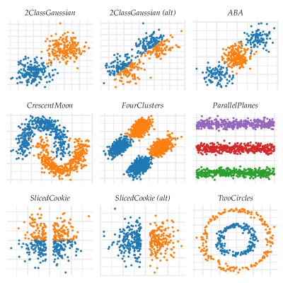
Figure 1: Simulated Datasets. Each can be generated using a function of the form generate*, where * should be replaced by the name of the dataset. (alt) indicates non-default parameters were used when calling the function.

2.2.2 Classifier Evaluation

To evaluate the performance of different methods, the package contains three types of functions that implement standard procedures for setting up such experiments. The first is by splitting a fully labeled dataset into a labeled set, an unlabeled set and a test set. For data in the form of a matrix, the split_dataset_ssl can be used. For data in the form of a data frame, the easiest way is to use magrittr’s pipe operator, splitting the data using the split_random command, using add_missinglabels_mar to randomly remove labels, and missing_labels or true_labels to recover these labels when we want to evaluate the performance on the unlabeled objects. The second type of experiment is to apply cross-validation in a semi-supervised setting using CrossValidationSSL. Distinct from the normal cross-validation setting, the data in the training folds get randomly assigned to the labeled or unlabeled set. The third type of experiment enabled by the package is to generate learning curves using the LearningCurveSSL function. These are performance curves for increasing numbers of unlabeled examples or an increasing fraction of labeled examples. For both the learning curves and cross-validation, multiple datasets can be given as input and the performance measures can be user defined, or one could use one of the supplied measure_* functions. Also in both cases, the experiments can optionally be run in parallel on multiple cores to speed up computation.

2.2.3 Plotting

Three ways to plot classifiers in simple 2D examples are provided. The most general method relies on the ggplot2 package [26] to plot the data and is provided in the form of the stat_classifier that can add classification boundaries to ggplot2 plots. geom_linearclassifier works in a similar way, but only works for a number of linear classifiers that have an associated line_coefficients method. Lastly, for these classifiers line_coefficients can be used directly to get the parameters that define the linear decision boundary, for use in a custom plotting function. In the examples, we will illustrate the use of stat_classifier and geom_linearclassifier.

3 Installation

The package is available from the Comprehensive R Archive Network (CRAN). As such, the easiest way to install the package is to run the following command using a recent version of R:

install.packages("RSSL")

The latest development version of the package can be installed using:

# If devtools is not installed run: install.packages("devtools")
devtools::install_github("jkrijthe/RSSL")

4 Examples

In this section, we will provide several examples of how the RSSL package can be used to illustrate or replicate results from the semi-supervised learning literature. Due to space constraints, we provide parts of the code for the examples in the text below. The complete code for all examples can be found in the source version of this document, which can be found on the author’s website.

4.1 A Failure of Self-Learning

While semi-supervised learning may seem to be obviously helpful, the fact that semi-supervised methods can actually lead to worse performance than their supervised counterparts has been both widely observed and described [4]. We will generate an example where unlabeled data is helpful (using the 2ClassGaussian problem from Figure 1) and one where unlabeled data actually leads to an increase in the classification error (2ClassGaussian (alt) in Figure 1), for the least squares classifier and self-learning as the semi-supervised learner. This can be done using the following code:

library(RSSL)
set.seed(1)

# Set the datasets and corresponding formula objects
datasets <- list("2 Gaussian Expected"=
                   generate2ClassGaussian(n=2000,d=2,expected=TRUE),
                 "2 Gaussian Non-Expected"=
                   generate2ClassGaussian(n=2000,d=2,expected=FALSE))
formulae <- list("2 Gaussian Expected"=formula(Class~.),
                 "2 Gaussian Non-Expected"=formula(Class~.))

# Define the classifiers to be used
classifiers <- list("Supervised" =
                      function(X,y,X_u,y_u) { LeastSquaresClassifier(X,y)},
                    "Self-learning" =
                      function(X,y,X_u,y_u) { SelfLearning(X,y,X_u,
                                                method = LeastSquaresClassifier)})

# Define the performance measures to be used and run experiment
measures <- list("Error" =  measure_error, "Loss" = measure_losstest)
results_lc <- LearningCurveSSL(formulae,datasets,
                           classifiers=classifiers,
                           measures=measures,verbose=FALSE,
                           repeats=100,n_l=10,sizes = 2^(1:10))

When we plot these results (using the plot method and optionally changing the display settings of the plot), we get the figure shown in Figure 2. What this shows is that, clearly, semi-supervised methods can be outperformed by their supervised counterpart for some datasets, for some choice of semi-supervised learner. Given that one may have little labeled training data to accurately detect that this is happening, in some settings we may want to consider methods that inherently attempt to avoid this deterioration in performance. We will return to this in a later example.

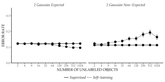
Figure 2: Example where self-learning leads to better performance as we add more unlabeled data (left) and increasingly worse performance as unlabeled data is added (right). The classifier used is the least squares classifier. The datasets are similar to the ones shown in Figure 1.

4.2 Graph Based Semi-supervised Learning

Many methods in semi-supervised learning attempt to use the assumption that labels change smoothly over dense regions in the feature space. An early attempt to encode this assumption is offered by [27] who propose to minimize an energy function for the labels of the unlabeled objects that penalizes large deviations between labels assigned to objects that are close, for some measure of closeness. This so-called harmonic energy formulation can also be interpreted as a propagation of the labels from the labeled objects to the unlabeled objects, through a graph that encodes a measure of closeness. We recreate [27]’s Figure 2, which can be found in Figure 3. Due to space constraints, we will defer the code to the online version of this document, since it is similar to the code for the next example.

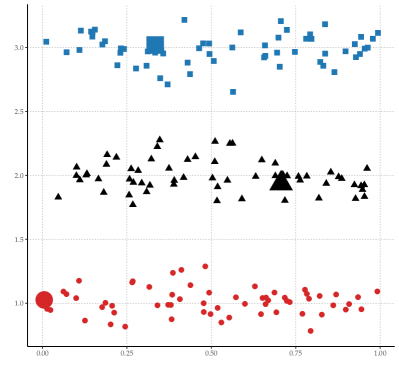
(a) Parallel planes dataset

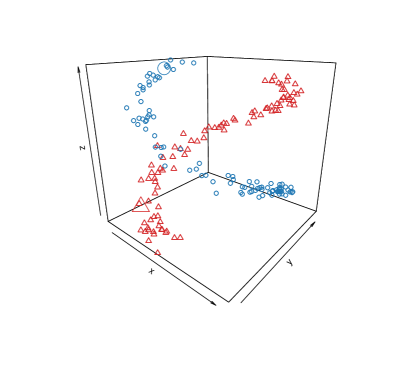
(b) Spirals dataset

Figure 3: Replication of Figure 2 from [27] demonstrating harmonic energy minimization. The larger points indicate the labeled objects. The color indicates the predicted class.

4.3 Manifold Regularization

Belkin et al. [1] build on the ideas of [27] by formulating the smoothness of the labeling function over the data manifold as a regularization term. In RSSL this Laplacian regularization term is included in both an SVM formulation and a regularized least squares formulation. For the Laplacian SVM formulation, Figure 2 from [1] provides an example of its performance on a simulated dataset. We can replicate this result using the following code. The results are shown in Figure 4.

library(RSSL)
library(dplyr)
library(ggplot2)
plot_style <- theme_classic() # Set the style of the plot

set.seed(2)
df_unlabeled <- generateCrescentMoon(n=100,sigma = 0.3) %>%
  add_missinglabels_mar(Class~.,prob=1)
df_labeled <- generateCrescentMoon(n=1,sigma = 0.3)
df <- rbind(df_unlabeled,df_labeled)

c_svm <- SVM(Class~.,df_labeled,scale=FALSE,
             kernel = kernlab::rbfdot(0.05),
             C=2500)

c_lapsvm1 <- LaplacianSVM(Class~.,df,scale=FALSE,
                         kernel=kernlab::rbfdot(0.05),
                         lambda = 0.0001,gamma=10)

c_lapsvm2 <- LaplacianSVM(Class~.,df,scale=FALSE,
                         kernel=kernlab::rbfdot(0.05),
                         lambda = 0.0001,gamma=10000)

# Plot the results 
# Change the arguments of stat_classifier to plot the Laplacian SVM
ggplot(df_unlabeled, aes(x=X1,y=X2)) +
  geom_point() +
  geom_point(aes(color=Class,shape=Class),data=df_labeled,size=5) +
  stat_classifier(classifiers=list("SVM"=c_svm),color="black") +
  ggtitle("SVM")+
  plot_style

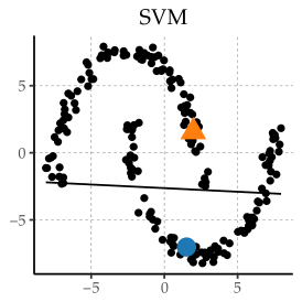
(a) $\lambda=0.0001$, $\gamma=0$

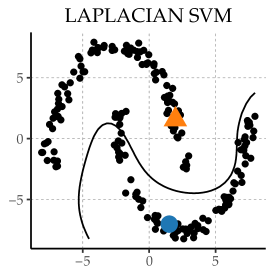
(b) $\lambda=0.0001$, $\gamma=10$

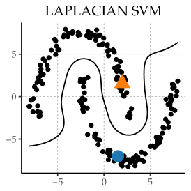
(c) $\lambda=0.0001$, $\gamma=10000$

Figure 4: Replication of Figure 2 from [1]. Laplacian SVM for various values of the influence of the unlabeled data.

4.4 Low Density Separation

A number of semi-supervised approaches attempt to leverage the assumption that the classification boundary may reside in a region of low-density. The Semi-supervised SVM or Transductive SVM [9] is one such approach. In [28, Chapter 6], an example is given for the potential problems this low-density assumption may cause when it is not valid by considering two artificial datasets. Here we replicate these results for a different classifier that makes use of the low-density assumption: entropy regularized logistic regression [7]. The results are shown in Figure 5. The code to generate these results can be found in the source version of this document.

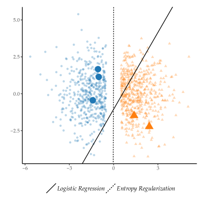
(a) Low-density assumption

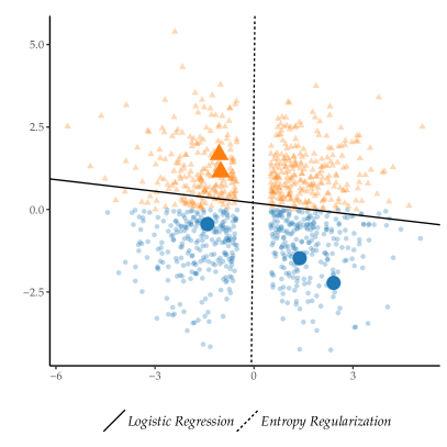
(b) Non low-density assumption

Figure 5: Demonstration of potential problems when the low density assumption does not hold, similar to Figure 6.5 in [28].

4.5 Improvement Guarantees

We now return to the example of deterioration in performance from Figure 2. The goal of our work in [18, 11, 12] is to construct methods that are guaranteed to outperform the supervised alternative. The guarantee that is given in these works is that the semi-supervised learner outperforms the supervised learner on the full, labeled and unlabeled, training set in terms of the surrogate loss (cf. [19]). The following code trains semi-supervised classifiers in these cases and returns the mean loss on the whole training set, the output is shown below the code example. It shows that indeed, these methods do not deteriorate performance in terms of the surrogate loss, while the self-learning method does show this deterioration in performance.

library(RSSL)
set.seed(1)

# Generate Example
df <- generate2ClassGaussian(n=1000, d=2, expected=FALSE)
df_semi <- add_missinglabels_mar(df, Class~., prob=0.995)

# Train and evaluate classifiers
mean(loss(LeastSquaresClassifier(Class~.,df_semi),df))
mean(loss(SelfLearning(Class~.,df_semi,method=LeastSquaresClassifier),df))
mean(loss(ICLeastSquaresClassifier(Class~.,df_semi),df))
mean(loss(ICLeastSquaresClassifier(Class~.,df_semi,
                          projection="semisupervised"),df))

## [1] 0.1763921
## [1] 0.4813863
## [1] 0.1185772
## [1] 0.1236701

5 Conclusion

We presented RSSL, a package containing implementations and interfaces to implementations of semi-supervised classifiers, and utility methods to carry out experiments using these methods. We demonstrated how the package can be used to replicate several results from the semi-supervised learning literature. More usage examples can be found in the package documentation. We hope the package inspires practitioners to consider semi-supervised learning in their work and we invite others to contribute to and use the package for research. Moreover, we hope the package contributes towards making semi-supervised learning research, and the research of those who use these methods in an applied setting, fully reproducible.

Acknowledgements.

This work was funded by project P23 of the Dutch public/private research network COMMIT.

References

- [1] Belkin, M., Niyogi, P., Sindhwani, V.: Manifold regularization: A geometric framework for learning from labeled and unlabeled examples. Journal of Machine Learning Research 7, 2399–2434 (2006)
- [2] Chang, C.C., Lin, C.J.: LIBSVM: a library for support vector machines. ACM Transactions on Intelligent Systems and Technology 2(3), 27 (2011)
- [3] Collobert, R., Sinz, F., Weston, J., Bottou, L.: Large scale transductive SVMs. Journal of Machine Learning Research 7, 1687–1712 (2006)
- [4] Cozman, F.G., Cohen, I., Cirelo, M.C.: Semi-Supervised Learning of Mixture Models. In: Proceedings of the 20th International Conference on Machine Learning. pp. 99–106 (2003)
- [5] Dempster, A., Laird, N., Rubin, D.: Maximum likelihood from incomplete data via the EM algorithm. Journal of the Royal Statistical Society. Series B 39(1), 1–38 (1977)
- [6] Eddelbuettel, D., Francois, R.: Rcpp : Seamless R and C ++ Integration. Journal of Statistical Software 40(1), 1–18 (2011)
- [7] Grandvalet, Y., Bengio, Y.: Semi-supervised learning by entropy minimization. In: Saul, L.K., Weiss, Y., Bottou, L. (eds.) Advances in Neural Information Processing Systems 17. pp. 529–536. MIT Press, Cambridge, MA (2005)
- [8] Hastie, T., Tibshirani, R., Friedman, J.H.: The Elements of Statistical Learning. Spinger, 2 edn. (2009)
- [9] Joachims, T.: Transductive inference for text classification using support vector machines. In: Proceedings of the 16th International Conference on Machine Learning. pp. 200–209. Morgan Kaufmann Publishers (1999)
- [10] Krijthe, J.H., Loog, M.: Implicitly Constrained Semi-Supervised Linear Discriminant Analysis. In: Proceedings of the 22nd International Conference on Pattern Recognition. pp. 3762–3767. Stockholm (2014)
- [11] Krijthe, J.H., Loog, M.: Optimistic Semi-supervised Least Squares Classification. In: Proceedings of the 23rd International Conference on Pattern Recognition (To Appear) (2016)
- [12] Krijthe, J.H., Loog, M.: Projected Estimators for Robust Semi-supervised Classification (2016), http://arxiv.org/abs/1602.07865
- [13] Krijthe, J.H., Loog, M.: Robust Semi-supervised Least Squares Classification by Implicit Constraints. Pattern Recognition 63, 115–126 (2017)
- [14] Li, Y., Tsang, I., Kwok, J., Zhou, Z.: Convex and Scalable Weakly Labeled SVMs. Journal of Machine Learning Research 14, 2151–2188 (2013), http://arxiv.org/abs/1303.1271
- [15] Li, Y.F., Zhou, Z.H.: Towards Making Unlabeled Data Never Hurt. IEEE Transactions on Pattern Analysis and Machine Intelligence 37(1), 175–188 (jan 2015)
- [16] Loog, M.: Constrained Parameter Estimation for Semi-Supervised Learning: The Case of the Nearest Mean Classifier. In: Machine Learning and Knowledge Discovery in Databases (Lecture Notes in Computer Science Volume 6322). pp. 291–304. Springer (2010)
- [17] Loog, M.: Semi-supervised linear discriminant analysis through moment-constraint parameter estimation. Pattern Recognition Letters 37, 24–31 (2014)
- [18] Loog, M.: Contrastive Pessimistic Likelihood Estimation for Semi-Supervised Classification. IEEE Transactions on Pattern Analysis and Machine Intelligence 38(3), 462–475 (2016)
- [19] Loog, M., Jensen, A.C.: Semi-Supervised Nearest Mean Classification through a constrained Log-Likelihood. IEEE Transactions on Neural Networks and Learning Systems 26(5), 995 – 1006 (2014)
- [20] McLachlan, G.J.: Iterative Reclassification Procedure for Constructing an Asymptotically Optimal Rule of Allocation in Discriminant Analysis. Journal of the American Statistical Association 70(350), 365–369 (1975)
- [21] Pedregosa, F., Varoquaux, G., Gramfort, A., Michel, V., Thirion, B., Grisel, O., Blondel, M., Prettenhofer, P., Weiss, R., Dubourg, V., Vanderplas, J., Passos, A., Cournapeau, D., Brucher, M., Perrot, M., Duchesnay, E.: Scikit-learn: Machine Learning in Python. Journal of Machine Learning Research 12, 2825–2830 (2011)
- [22] R Core Team: R: A Language and Environment for Statistical Computing. R Foundation for Statistical Computing, Vienna, Austria (2016), https://www.r-project.org/
- [23] Shaffer, J.P.: The Gauss-Markov Theorem and Random Regressors. The American Statistician 45(4), 269–273 (1991)
- [24] Sindhwani, V., Keerthi, S.S.: Large scale semi-supervised linear SVMs. In: Proceedings of the 29th Annual International ACM SIGIR Conference on Research and Development in Information Retrieval. pp. 477–484. ACM (2006)
- [25] Webb, A.: Statistical Pattern Recognition. John Wiley & Sons, 2 edn. (2002)
- [26] Wickham, H.: ggplot2: Elegant Graphics for Data Analysis. Springer-Verlag New York (2009), http://ggplot2.org
- [27] Zhu, X., Ghahramani, Z., Lafferty, J.: Semi-supervised learning using gaussian fields and harmonic functions. In: Proceedings of the 20th International Conference on Machine Learning. pp. 912–919 (2003)
- [28] Zhu, X., Goldberg, A.B.: Introduction to Semi-Supervised Learning. Morgan & Claypool (2009)