RNA substructure as a random matrix ensemble

Abstract

Combinatorial analysis of a certain abstraction of RNA structures has been studied to investigate their statistics. Our approach regards the backbone of secondary structures as an alternate sequence of paired and unpaired sets of nucleotides, which can be described by random matrix model. We obtain the generating function of the structures using Hermitian matrix model with Chebyshev polynomial of the second kind and analyze the statistics with respect to the number of stems. To match the experimental findings of the statistical behavior, we consider the structures in a grand canonical ensemble and find a fugacity value corresponding to an appropriate number of stems.

I Introduction

Ribonucleic acid (RNA) is a single strand of nucleotides, each of which is one of the four bases, A, U, C and G. The base pairs are made intra-molecularly, leading the backbone of nucleotides to form a 3-dimensional structure called the tertiary structure. Since the functional role of an RNA is determined by its tertiary structure, the prediction of the tertiary from the sequence of nucleotides is of great interest Higgs (2000); Fallmann et al. (2017).

As an intermediate stage, the secondary structure is a planar structure which allows only nested base pairs. The meaning of the nested base pairs is evident when the secondary structure is represented as a labeled graph over the vertex set $\{1,2,\cdots,n\}$ (Fig.1): the sequence of vertices $(1,2,\cdots,n)$ is put on a horizontal line. The horizontal line represents the backbone and each vertex denotes the nucleotide. The base pairs are drawn as arcs in the upper half-plane. In terms of the graph, the nested base pairs mean non-crossing arcs. Another important feature of secondary structures is that a base pair between adjacent two nucleotides (called 1-arc) is not allowed due to the rigidity of the backbone. In other words, any two vertices require at least one unpaired vertex between them to pair to each other.

Since the secondary interactions are in general stronger than tertiary interactions such as crossing base pairs (called pseudoknots) or base triples, the prediction of secondary structures has been intensively studied as a scaffold to the tertiary Nussinov and Jacobson (1980); Zuker and Stiegler (1981); Zuker and Sankoff (1984); Rivas and Eddy (1999); Schuster et al. (1997). The most common approach is the free energy minimization. The energy of the structures is lower as base pairs are formed and it is assumed that structures tend to be thermodynamically stable.

Figure 1: Secondary structure and its equivalent graph.

On the other hand, combinatorial approaches have also played an important role in better understanding the RNA structures. The structures are often considered as combinatorial objects such as the graph in Fig.1, regardless of the types of bases. Combinatorial analysis are then applied to enumerate such objects under various kinds of restrictions and classifications, which help to develop and advance the prediction algorithms Waterman (1978); Hofacker et al. (1998); Li and Reidys (2016).

In this paper, we investigate a certain substructure of the secondary structure from the combinatorial point of view, using the Hermitian random matrix model. The matrix model was first introduced in RNA structures to deal with the pesudoknots Vernizzi et al. (2005); Andersen et al. (2013a, b). since its topological expansion facilitates the enumeration of pseudoknot structures under a topological classification. The underlying relation between the matrix model and RNA structures is established by a diagrammatic representation of the matrix model. Although we also employ the matrix model, we consider here only planar structures and the diagrammatic representation is mainly used to describe our substructures.

Before introducing the substructure, let us first define auxiliary concepts required to describe the substructure. An island is defined as a set of maximally consecutive paired nucleotides while a bridge is a set of maximally consecutive unpaired nucleotides. Consequently, the backbone of the secondary structure is represented as an alternate sequence of island and bridge. Then the total number of nucleotides $\sum_{i=1}^{I}(\ell_{i}+b_{i})$ where $\ell_{i}$ and $b_{i}$ are the number of nucleotides in the $i$-th island and bridge, respectively where we identify the bridge before the first island with the one after the last island for convenience. We remark here that the condition of 1-arc forbidden in the secondary structures implies an important feature of the island, which is that there is no base pair between vertices inside one island by definition.

It is usual to analyze the combinatorics of the secondary structures with the total number of nucleotides fixed. However, in this paper, we are interested in the combinatorics of the structures for a given number of base pairs, regardless of the number of unpaired nucleotides. Thus, we introduce a substructure ignoring the unpaired ones. The structure which we call island diagram is obtained from the secondary structure by representing each bridge as a single blank (Fig.2). Accordingly, the island diagram retains the configuration of base pairs and unpaired regions, but is the abstract structure of the secondary structures with different number of nucleotides in the unpaired regions.

Figure 2: The island diagram derived from the secondary structure given in Fig.1. Each island is depicted as a line segment. Each bridge is represented as a blank in the island diagram. A bridge, of which left and right vertices are paired to each other, is called the hairpin loop. The two encircled bridges are the hairpin loops.

The paper is organized as follows. In section II, we establish the relation between the matrix model and the island diagrams. The generating function enumerating island diagrams is obtained using the matrix model description. In section III, we investigate a distribution of island diagrams, which disagrees with the one expected from the energy minimization scheme. A parameter analogous to the chemical potential is introduced to fit the distribution and we give a possible interpretation to the parameter. Section IV discusses possible extensions of the island diagram configuration and section V is the conclusion.

II Theory

II.1 Matrix model description

We employ Hermitian matrix model to describe and enumerate the island diagrams. The combinatorial aspect of the matrix model is based on its diagrammatic representation, which is often called Feynman diagram. In this section, we present the connection between the matrix model diagrams and island diagrams.

Let us first briefly review the diagrams generated by the matrix model. The Gaussian expectation value of an operator $O(M)$ is written as

$$\left\langle{O(M)}\right\rangle:=\frac{1}{Z}\int dM\,\,O(M)\,e^{-\frac{N}{2}\mathrm{Tr}M^{2}}$$ (1)

where $M$ is $N\times N$ Hermitian matrix and $Z$ is the normalization factor requiring $\left\langle{1}\right\rangle=1$. It is well-known that the expectation value can be formulated pictorially. Let us see this through the example of $O(M)=N\,\mathrm{Tr}M^{k}$. The $\mathrm{Tr}M^{k}$ corresponds to a vertex of $k$ double line half-edges with a cyclic ordering (Fig.3(a)) (not to be confused with the vertex representing a nucleotide in the secondary structures). The Gaussian integral indicates pairing the half-edges with the propagator, represented as the double line edge (Fig.3(b)).

Figure 3: (a) Vertex of $k$ half-edges. (b) Propagator.

A diagram obtained by pairing all the half-edges is called the fatgraph and the expectation value counts the number of fatgraphs.

The advantage of the matrix model is its topological expansion, namely, it counts the number of fatgraphs filtered with their genus. The genus $g$ of a fatgraph is determined from its Euler characteristic $\chi=2-2g=v-e+f$ where $v$, $e$ and $f$ are the number of vertices, edges and faces (loops), respectively. The genus filtration appears in the expectation value as the factor $N^{\chi}$ (for rigorous computations and arguments, see for instance Di Francesco (1999)). As an explicit example, in the case of $O(M)=N\,\mathrm{Tr}M^{4}$, the result is given by $2N^{2}+N^{0}$ that is pictorially described in Fig.4.

Figure 4: Diagrammatic representation of the expectation value of $M^{4}$.

The term $2N^{2}$ reads the two planar diagrams and $N^{0}$ reads the non-planar (torus) diagram.

In order to see the connection between the fatgraphs and island diagrams clearly, it is more convenient to use dual graphs of the matrix model diagrams. Given a fatgraph of the matrix model, its dual graph is obtained by transforming the vertex of $k$ half-edges into the horizontal line of $k$ vertices. In other words, the vertex is stretched out to form the horizontal line (Fig.5).

Figure 5: Transformation of a fatgraph into its dual.

In the dual representation, therefore, the expectation value of $\mathrm{Tr}M^{4}$ is described as in Fig.6.

Figure 6: Dual representation of the diagrams in Fig.4.

Let us now find the matrix model description to represent the island diagrams. It is obvious that we need only genus zero contributions in the topological expansion of the matrix model since the secondary structures are the planar structures. The next step is to find the way to impose the configuration of islands on the matrix model diagrams. Let us consider the number $I$ of islands each of which has $k_{a}\geq 1$ vertices for $a\in\{1,\cdots,I\}$ with $k=k_{1}+\cdots+k_{I}$. We may first try with $\big{\langle}\mathrm{Tr}\prod_{a=1}^{I}M^{k_{a}}\big{\rangle}_{0}$ where the subscript $0$ denotes genus zero contributions. Here $M^{k_{a}}$ corresponds to $k_{a}$ half-edges among $k$. The expectation value is merely rewriting of $\left\langle{\mathrm{Tr}M^{k}}\right\rangle_{0}$ and hence generates all possible planar diagrams paring $k$ vertices.

However, some of the planar diagrams may not be allowed as island diagrams. One can see this clearly through the example of $\left\langle{\mathrm{Tr}MM^{2}M}\right\rangle_{0}$, which generates the first two planar diagrams in Fig.6. Meanwhile, the island configuration we have in mind by rewriting $M^{4}$ into $MM^{2}M$ is 3 islands with 1, 2 and 1 vertices. Then, the two planar diagrams are interpreted as the graphs in Fig.7.

Figure 7: Graphs described by $MM^{2}M$. The graph on the right hand side is not the island diagram due to the 1-arc in the middle.

Recall that, however, secondary structures do not allow 1-arc and hence any base pair is forbidden on one island. Therefore, the second graph in Fig.7 should be excluded from the island diagrams.

In order to impose the constraint, we introduce $U^{(k_{a})}(M)$ instead of $M^{k_{a}}$ as an operator corresponding to the island with $k_{a}$ vertices and consider the expectation value of

$$O^{(I)}_{\{k_{a}\}}=\mathrm{Tr}\prod_{a=1}^{I}U^{(k_{a})}(M)\,.$$ (2)

To find the faithful expression for $U^{(k_{a})}$, we need to impose the condition of 1-arc absent on an island. This can be done by means of the inclusion-exclusion method, which gets rid of diagrams with 1-arcs step by step. The operator $M^{n}$ reduces to $M^{n-2}$ after removing 1-arc paring. The number of ways of assigning one 1-arc is $n-1$. Note that the expectation value of $M^{n-2}$ generates all the diagrams having the 1-arc from $M^{n}$. Therefore, we subtract those configurations and introduce the operator $M^{n}-(n-1)M^{n-2}$. However, in which case, the diagrams with two 1-arcs are over-subtracted and need to be compensated by adding the term $M^{n-4}$. In this way, adding/subtracting $M^{n-2p}$ with the number of possible contractions of $p$ 1-arcs, we arrive at the final result,

$$U^{(n)}(M)=\sum_{p=0}^{\lfloor n/2\rfloor}(-1)^{p}\binom{n-p}{p}M^{n-2p}\,.$$ (3)

Finally, we find a simple integration formula for the expectation value by identifying the polynomial $U^{(n)}$ with the Chebyshev polynomial of the second kind $U_{n}$, $U^{(n)}(2\xi)=U_{n}(\xi)$. The Chebyshev polynomial has the product rule,

$$U_{m}(\xi)U_{n}(\xi)=\sum_{k=0}^{n}U_{m-n+2k}(\xi)~{}~{}~{}~{}\mathrm{for}~{}~{}~{}n\leq m,$$ (4)

and, therefore, the vertex operator $O^{(I)}_{\{k_{a}\}}$ in (2) ends up with the linear combination of Chebyshev polynomials. Note that $\big{\langle}\mathrm{Tr}U_{n}(M/2)\big{\rangle}_{0}=0$ unless $n=0$ due to the constraint of 1-arc absence. Therefore, the expectation value of $O^{(I)}_{\{k_{a}\}}$ is given as the coefficient of $U_{0}=1$,

$$\big{\langle}O^{(I)}_{\{k_{a}\}}\big{\rangle}_{0}=\frac{2}{\pi}\int_{-1}^{1}\prod_{a=1}^{I}U_{k_{a}}(\xi)U_{0}(\xi)\sqrt{1-\xi^{2}}d\xi$$ (5)

where the orthonormality of the Chebyshev polynomials is used:

$$\int_{-1}^{1}U_{k}(\xi)U_{\ell}(\xi)\sqrt{1-\xi^{2}}d\xi=\frac{\pi}{2}\delta_{k,\ell}.$$ (6)

II.2 Generating functions

Based on the integration formula (5), we can find the generating function of the island diagrams. We first classify the island diagrams by the number of islands, basepairs, and hairpin loops. A hairpin loop is defined as a bridge, of which veritces on the left and right adjacent islands are connected to each other (Fig.1).

Let us denote by $g(h,I,\ell)$ the number of island diagrams with $h$ hairpins, $I$ islands and $\ell$ basepairs. It is easy to find $g(h,I,\ell)$ if one uses a property of hairpin loop. Observe that there must be at least one hairpin loop between two nucleotides at each end of a basepair. Therefore, we may regroup islands between two consecutive hairpin loops as one effective island since there is no basepair connected inside an effective island (Fig.8).

Figure 8: Example of effective island. The three islands encircled by the dashed line is one effective island.

The number of ways to make an effective island consisting of $I_{a}$-islands and $k_{a}$-nucleotides is given by $\binom{k_{a}-1}{I_{a}-1}$. Since there are $h+1$ effective islands, one concludes that

$$g(h,I,\ell)= \sum_{\{k_{a},I_{a}\}}\prod_{a=1}^{h+1}\binom{k_{a}-1}{I_{a}-1}$$

$$\times\left\langle{\mathrm{Tr}\,U_{k_{1}-1}\prod_{j=2}^{h}U_{k_{j}-2}\,U_{k_{h+1}-1}}\right\rangle_{0}$$ (7)

where $k_{a}$ and $l_{a}$ are constrained as $k_{1}+\cdots+k_{h+1}=2\ell$ and $I_{1}+\cdots+I_{h+1}=I$. This complicated expression is simplified if one uses the generating function of the Chebyshev polynomial,

$$\sum_{k\geq 0}\sum_{i=0}^{k}\binom{k}{i}\,z^{k/2}\,y^{i}\,U_{k}(\xi)=\frac{1}{1-2\sqrt{z}(1+y)\xi+z(1+y)^{2}}\,.$$ (8)

Then the integral expression in (7) is put into a compact form of the generating function,

$$G(x,y,z):=\sum_{h,I,\ell}g(h,I,\ell)x^{h}y^{I}z^{\ell}$$ (9)

$$=\sum_{h}\frac{2}{\pi}\int_{-1}^{1}\frac{\sqrt{1-\xi^{2}}}{\left(1-2\sqrt{z}(1+y)\xi+z(1+y)^{2}\right)^{h+1}}d\xi\,.$$

One can calculate the integral for given $h$ and obtain

$$G(x,y,z)= \sum_{h}x^{h}\,z^{h}\,y^{h+1}\,(1+y)^{h-1}$$

$$~{}~{}~{}\times{}_{2}F_{1}(h+1,h;2;z(1+y)^{2}).$$ (10)

Here ${}_{2}F_{1}(a,b;c;z)$ is the hypergeometric function and can be written as ${}_{2}F_{1}(h+1,h;2;z)=\sum_{k\geq 0}N(h+k,h)z^{k}$ where $N(a,b)=\frac{1}{a}\binom{a}{b}\binom{a}{b-1}$ is the Narayana number whose generating function is known (see for instance Barry and Hennessy (2011)). Therefore, one can rewrite $G(x,y,z)$ in the closed form

$$G(x,y,z)=\left(\frac{y}{1+y}\right)$$ (11)

$$~{}~{}\times\frac{1-A(1+B)-\sqrt{1-2A(1+B)+A^{2}(1-B)^{2}}}{2A}$$

where $A=z(1+y)^{2}$ and $B={x\,y}/(1+y)$.

The power series of the generating function provides the information on $g(h,I,\ell)$ which will be the building block of other generating functions. For example, to investigate further details of the secondary structures, one may introduce the concept of stem (or stack) defined as a set of maximally consecutive parallel basepairs. The length of a stem is the number of basepairs in the stem. Let us add one more variable, the number $k$ of stems to $g(h,I,\ell)$ so that the number of configurations together with stems are denoted by $f(k,h,I,\ell)$. Finding $f(k,h,I,\ell)$ is based on the number of single-stack diagrams, where we define the single-stack diagram as the island diagrams that consists of only stems of stack-length one. Namely, each stem is itself a basepair in the single-stack diagrams. Let $s(h,I,k)$ denotes the number of the single-stack diagrams of $k$ stems. The structures of $k$ stems and $\ell$ basepairs can be constructed by stacking $\ell-k$ basepairs on each stem of the single-stack diagrams. Therefore, we have the relation

$$f(k,h,I,\ell)=\binom{\ell-1}{k-1}\,s(h,I,k)\,.$$ (12)

This shows that the generating function $F(u,x,y,z):=\sum_{k,h,I,\ell}f(k,h,I,\ell)\,u^{k}x^{h}y^{I}z^{\ell}$ is given as

$$F(u,x,y,z)=S\Big{(}x,y,\frac{u\,z}{1-z}\Big{)}\,.$$ (13)

where $S(x,y,z):=\sum_{h,I,\ell}s(h,I,\ell)\,x^{h}y^{I}z^{\ell}$. Finally, noting that $F(1,x,y,z)=G(x,y,z)$, one finds $S(x,y,z)=G(x,y,{z}/(1+z))$ and therefore,

$$F(u,x,y,z)=G\Big{(}x,y,\frac{u\,z}{1+u\,z-z}\Big{)}\,.$$ (14)

III Application

Let us investigate the result of the generating functions. We consider here the stem distribution of island diagrams for given numbers of basepairs. Using $f(k,h,I,\ell)$, one may define $\Omega_{k,\ell}=\sum_{h,I}f(k,h,I,\ell)$ which represents the number of island diagrams with $k$ stems and $\ell$ basepairs. From (10) and (14), one finds the explicit formula

$$\Omega_{k,\ell}=\binom{\ell-1}{k-1}\sum_{p=0}^{\lfloor\frac{k-1}{2}\rfloor}M(k-1,p)~{}2^{3p}\,5^{k-2p-1}$$ (15)

where $M(\alpha,\beta):=\frac{\alpha!}{(\alpha-2\beta)!\,\beta!\,(\beta+1)!}$ is the Motzkin polynomial coefficient Motzkin (1948); Donaghey and Shapiro (1977). For a given value of $\ell$, one can plot $\Omega_{k,\ell}$ as a function of $k/\ell$ to see the stem distribution (square marks in Fig.9 for $\ell=100$). The most probable value appears near $k/\ell=1$.

On the contrary, according to the experimental findings, the average basepair per stem in the secondary structures is in general greater than two, that is, $k/\ell<1/2$. The noticeable difference in the average value of $k/\ell$ tells that the stem distribution of secondary structures is not driven solely by the multiplicity of possible structures. In fact, it is known that the secondary structures obtained by energy minimizations tend to have more basepairs per stem than that is expected from combinatorics Hofacker et al. (1998). This is mainly because, from the energy point of view, a stack of basepairs contributes to the stability of the stem in such a way that a longer stem is preferred.

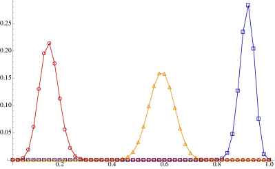
Figure 9: Normalized distribution $\Omega_{k,\ell}\,e^{\mu\,k}/(\sum_{k}\Omega_{k,\ell}\,e^{\mu\,k})$ of island diagrams as a function of $k/\ell$ for $\ell=100$: Square($\mu=0$), triangle($\mu=-2$), circle($\mu=-4$).

In order to take account of the stack stability in combinatorial approaches, it is usual to consider so-called $r$-canonical structures, which are the structures without a stem of length less than $r$ Barrett et al. (2016). Assuming such short stems are energetically unstable, one may exclude the structures with the short stems and investigate the space of only $r$-canonical structures from the outset. The $r$-canonical island diagrams can be built up from the single-stack diagrams by assigning $r-1$ more basepairs at each stem from the beginning:

$$F(u\,z^{r-1},x,y,z)=G\Big{(}x,y,\frac{u\,z^{r}}{1+u\,z^{r}-z}\Big{)}\,.$$ (16)

On the other hand, however, one may consider another way that allows short stems, but with a certain weight reflecting their instability. The weight can be imposed on the number of stems $k$ since the length of each stem decreases as $k$ increases for given $\ell$. We introduce $e^{\mu}$ as the weight and put it in the generating function as

$$F(u\,e^{\mu},x,y,z)=G\Big{(}x,y,\frac{u\,z\,e^{\mu}}{1+u\,z\,e^{\mu}-z}\Big{)}$$ (17)

which is equivalent to replacing $\Omega_{k,\ell}$ with $e^{\mu k}\Omega_{k,\ell}$. One may find the system analogous to the grand canonical ensemble. The weight is the fugacity with $\mu$ playing the role of the chemical potential related to creating stems. Regarding $\log\Omega_{k,\ell}$ as entropy, one has $\mu=-\frac{\partial}{\partial k}\log\Omega_{k,\ell}$ at the maximum. Depending on the value of $\mu$, one finds the peak value $k_{0}$ of $\Omega_{k,\ell}$ shifted (triangle or circle marks in Fig.9). The database Andronescu et al. (2008) shows that RNA molecules tend to have the average stack length per stem in the range from 2 to 10, mostly near $4$ independent of $\ell$. Referring to this, one may require $k_{0}/\ell$ to be in the range from 1/5 to 1/3 and finds $\mu$, linearly fitted as (Fig.10)

$$\mu(k_{0})\simeq-4.7+5.0\,k_{0}/\ell$$ (18)

whose number is only slightly changed as $\ell$ varies.

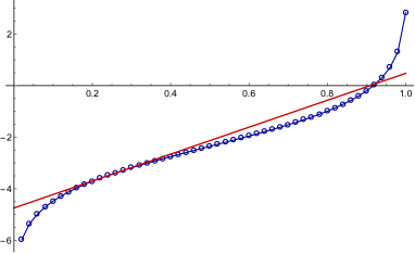
Figure 10: Chemical potential $\mu$ as a function of the peak value $k_{0}/\ell$ for $\ell=100$. The linear fitting is shown for the range from 1/5 to 1/3.

This idea is tested using the data obtained from Andronescu et al. (2008). The number of RNA molecules is given by a histogram as a function of $k/\ell$ where we set the interval of the bin to be 0.02 (Fig.11) and require $\ell\geq 50$ so that at each bin the data is not empty. The total number of collected data turns out to be 335 from Andronescu et al. (2008) and they are distributed as 283 ($50\leq\ell<150$) and 52 ($150\leq\ell$). The best sample will be the data set with given $\ell$. However, we cannot get a significant number of data set with a given $\ell$. To overcome the statistical error, we use the whole data set with $\ell\geq 50$ assuming different $\ell$ of the data set does not affect much of the result. The histogram shows $0.22\leq k_{0}/\ell<0.24$ and therefore, $\mu\simeq-3.6$. For comparison, the normalized distributions corresponding to $\mu=-3.6$ are plotted using the generating function when $\ell=50$(circle), $100$(triangle), $200$(square). Different $\ell$ shows only the slight change of the standard deviation which confirms the assumption.

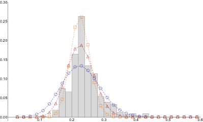
Figure 11: Histogram of RNA for $\ell\geq 50$ obtained from Andronescu et al. (2008) as a function of $k/\ell$. Normalized distributions $\Omega_{k,\ell}\,e^{\mu\,k}/(\sum_{k}\Omega_{k,\ell}\,e^{\mu\,k})$ for $\mu=-3.6$ when $\ell=50$(circle), $100$(triangle), $200$(square) are given for comparison.

One way of interpreting the chemical potential from the perspective of usual energy model is the stacking energy of base pairs. It is believed that the attractive energy between two consecutive base pairs is the main contribution to the stability of the stem. The stacking energy depends not only on the nucleotides involved but also on the stacking order of the two pairs along the backbone Freier et al. (1986). Nevertheless, if we assume an average stacking energy $\epsilon$ at some fixed temperature, we may have additional statistical factor $e^{\epsilon(\ell-k)}$ to $\Omega_{k,\ell}$ for the given structures with $k$ stems and $\ell$ basepairs. When we consider the distribution for fixed $\ell$, the factor $e^{\epsilon\ell}$ cancels out by the normalization. Therefore, one may view the chemical potential as the average stacking energy, $\mu=-\epsilon$. We remark that the number of ways putting unpaired nucleotides on bridges can significantly change the value of $\epsilon$. The value $-3.6$ of $\mu$ should be considered as the one evaluated under the reference point that an appropriate number of unpaired nucleotides is already assigned on the bridges.

Another way is to understand the stack stability in terms of the multiplicity of structures from the pure combinatorial point of view. Recall that an island diagram is in general the abstract structure of numerous secondary structures. In this respect, one may interpret the factor $e^{\mu k}$ as the one reflecting the number of secondary structures which reduce to the island diagrams for a given $k$. In other words, the fugacity quantifies how fast the multiplicity of secondary structures decreases as $k$ increases.

IV Possible extensions

In this section, we remark on some extensions and possible applications by presenting brief descriptions without giving much detail. Firstly, we mention that the relation between island diagrams and RNA abstract shapes, which are provided in Giegerich et al. (2004) to classify secondary structures according to their structural similarities. In particular, the single-stack diagram is directly related to $\pi^{\prime}$-shape. Given a secondary structure, its $\pi^{\prime}$-shape is obtained as follows: each stem is replaced by a single basepair. And each group of maximally consecutive unpaired bases is represented as a single unpaired region, regardless of the number of unpaired bases in it (refer to Giegerich et al. (2004); Lorenz et al. (2008) for its formal definition and details). The unpaired regions corresponds to the bridges so that the single-stack diagrams are indeed the $\pi^{\prime}$-shapes. The only difference is that, in island diagrams, we identify the bridge before the first island with the one after the last island just for convenience. Therefore, the generating function of single-stack diagrams can immediately be applied to $\pi^{\prime}$-shapes and one obtains $(1+y)^{2}S(x,y,z)/y$. Here, $x$ and $z$ are the expansion variables for the number of hairpins and basepairs(stems), respectively, whereas $y$ now stands for the expansion variable of bridges. The factor $(1+y)^{2}$ reflects the possible four cases of putting bridges at the two ends of the backbone.

Although we have dealt with abstract structures ignoring the number of unpaired bases to analyze statistics for given $\ell$, it is easy to derive the generating function with the total number of bases from the island diagrams by simply putting the unpaired bases in bridges. Let us introduce one more expansion variable $w$ corresponding to the number of bases. The procedure is as follows: first, the number $I-1-h$ of bridges between islands (excluding hairpin loops and two bridges at the end of backbone) must contain at least one nucleotide, which will give the factor $w^{I-1-h}$. Second, each basepair has two nucleotides that implies the factor $w^{2\ell}$ for given $\ell$. Third, there are $I+1$ bridges on the backbone and one may put arbitrary number of nucleotides on each bridge, which introduces the factor $1/(1-w)^{I+1}$. In addition to this, one may introduce the constraint that each hairpin loop consists of at least $\lambda-1$ nucleotides, which reflects the rigidity of the backbone. This constraint shifts the variable $x$ to $xw^{\lambda-1}$. As a result, the generating function of a given number of nucleotides can be obtained from the previous generating functions by replacing the variables $x\to xw^{\lambda-2}$, $y\to yw/(1-w)$, $z\to zw^{2}$ and multiplying the overall factor $1/(w(1-w))$. For instance, one obtains $r$-canonical generating function $R_{\lambda}(u\,z^{r-1},x,y,z;w):=\sum_{k,h,I,\ell,n}r_{\lambda}(k,h,I,\ell;n)\,u^{k}x^{h}y^{I}z^{\ell}w^{n}$,

$$R_{\lambda} (u\,z^{r-1},x,y,z;w)$$ (19)

$$=\frac{1}{w(1-w)}F\bigg{(}u(zw^{2})^{r-1},xw^{\lambda-2},\frac{y\,w}{1-w},zw^{2}\bigg{)}\,.$$

One can check that the generating function $R_{\lambda}(z^{r-1},1,1,z;w)$ agrees with the one $S_{\lambda}^{[r]}(w,z)$ appeared in Barrett et al. (2016) where stems, hairpin loops and islands are not the observables.

Finally, we want to remark here on an interesting possible application. The configuration of island diagrams is seen to have a close relation to the model of polydisperse chains on a one-dimensional lattice Stilck et al. (2006). In the model, a chain with the number $M$ of monomers is placed on a lattice in such a way that one monomer of the chain occupies one lattice point. The polydisperse system consists of numerous chains having diverse sizes placed on a lattice (Fig.12).

Figure 12: A particular configuration in a polydisperse system that consists of three chains with 4, 2 and 3 monomers on the lattice with 14 sites. The empty circles represent empty sites.

In Stilck et al. (2006), the entropy of the system and the distribution of chain sizes are calculated as a function of the density of monomers when the lattice length is taken to be large.

One can immediately make an analogy between the polydisperse system and the island diagrams. When only the sequence of islands without base pairs is taken into account, an island of length $M$ corresponds to a chain with $M$ monomers and the number of islands matches up with the number of chains. The number of nucleotides is the lattice length and unpaired ones are empty sites on the lattice such that the density of monomers is the density of paired ones. Having the analogy in mind, let us briefly illustrate the generating functions for the polydisperse system. Let $\mathfrak{g}(I,L)$ denote the number of configurations with $I$ chains(islands) and $L$ monomers(paired bases). Since there are no concepts of hairpins or base pairs, $\mathfrak{g}(I,L)$ is just given by the summation of $1$ over $k_{1}+\cdots+k_{I}=L$ such that its generating function is given as

$$\mathfrak{G}(y,z):=\sum_{I,L\geq 0}\,\sum_{k_{1}+\cdots+k_{I}=L}y^{I}\,z^{L}=\frac{1}{1-\frac{y}{1-z}}\,.$$ (20)

Now we take empty sites(unpaired bases) into account by putting them between chains. The polydisperse system has no restrictions on the minimum number of empty sites between chains and hence it is simpler than the case of island diagrams given above. Referring to the above procedure, one may easily find the generating function,

$$\mathfrak{R}(y,z;w):=\sum_{I,L,N}\mathfrak{r}(I,L;N)y^{I}z^{L}w^{N}=\frac{1}{1-w-\frac{yzw}{1-zw}}\,.$$ (21)

where $\mathfrak{r}(I,L;N)$ denotes the number of configurations with $I$ chains, $L$ monomers and $N$ lattice length(total number of nucleotides).

One may exploit the generating function to find asymptotic behaviors of the coefficients when the lattice length is taken to infinity and reproduce known results given in Stilck et al. (2006) such as the distribution of chain sizes. Furthermore, it will be an amusing study to consider the role of base pairs in connection with the system of chains. In particular, the concept of hairpins may have an immediate application as is related to an interaction between adjacent chains.

V Conclusion

We considered the island diagrams which are the abstraction of RNA secondary structures. The island diagram is introduced to study combinatorics of the secondary structures for a given number of base pairs, rather than for a given number of nucleotides. Using the Hermitian matrix model with the help of Chebyshev polynomial, we can derive various generating functions of the structures in a closed form. In addition, we introduced the fugacity to match the experimental finding of average number of basepairs in a stem. As a result, we evaluated the chemical potential of the stem from the combinatorial approach. Finally, we also suggested possible extensions of the island diagrams. In particular, the application to the model of polydisperse chains will be of interest.