Asteroid 1566 Icarus’s size, shape, orbit, and Yarkovsky drift from radar observations

Abstract

Near-Earth asteroid (NEA) 1566 Icarus ($a=1.08$ au, $e=0.83$, $i=22.8^{\text{$\circ$}}$) made a close approach to Earth in June 2015 at 22 lunar distances (LD). Its detection during the 1968 approach (16 LD) was the first in the history of asteroid radar astronomy. A subsequent approach in 1996 (40 LD) did not yield radar images. We describe analyses of our 2015 radar observations of Icarus obtained at the Arecibo Observatory and the DSS-14 antenna at Goldstone. These data show that the asteroid is a moderately flattened spheroid with an equivalent diameter of 1.44 km with 18% uncertainties, resolving long-standing questions about the asteroid size. We also solve for Icarus’ spin axis orientation ($\lambda=270^{\text{$\circ$}}\pm 10^{\text{$\circ$}},\beta=-81^{\text{$\circ$}}\pm 10^{\text{$\circ$}}$), which is not consistent with the estimates based on the 1968 lightcurve observations. Icarus has a strongly specular scattering behavior, among the highest ever measured in asteroid radar observations, and a radar albedo of $\sim$2%, among the lowest ever measured in asteroid radar observations. The low cross-section suggests a high-porosity surface, presumably related to Icarus’ cratering, spin, and thermal histories. Finally, we present the first use of our orbit determination software for the generation of observational ephemerides, and we demonstrate its ability to determine subtle perturbations on NEA orbits by measuring Icarus’ orbit-averaged drift in semi-major axis ($(-4.62\pm 0.48)\times 10^{-4}$ au/My, or $\sim$60 m per revolution). Our Yarkovsky rate measurement resolves a discrepancy between two published rates that did not include the 2015 radar astrometry.

I. Introduction

Earth-based radar is a powerful tool for determining surface, subsurface, and dynamical properties of objects within the Solar System. Radar imaging has been used to obtain high-resolution images of planets, moons, asteroids, and comets, as well as constrain their orbits and spin pole orientations. In particular, radar is the only remote observing method, other than a physical flyby mission, which can obtain multiple-aspect, sub-decameter shape data for minor planets.

Radar is particularly useful for studying Near-Earth Objects (NEOs). As fragments of leftover planetesimals, NEOs serve as a window into the processes that governed the formation of the Solar System. NEO studies probe the accretional, collisional, erosional, radiative, and tidal processes which shape the continued evolution of the minor planets. Determination of NEO orbits and gravity environments opens the door to human exploration of these objects, including potentially valuable sample return missions. Arguably most important of all, the discovery, categorization, and orbit determination of NEOs, as mandated by the United States’ Congress, helps identify those objects which are potentially hazardous to life on Earth.

The first asteroid radar observations occurred at Haystack on June 13–15, 1968 (Pettengill et al., 1969) and Goldstone on June 14–16, 1968 (Goldstein, 1969), during a 16 lunar distance (LD) close approach of the object 1566 Icarus. Icarus’ highly elliptical orbit ($a=1.08$ au, $e=0.83$, $i=22.8^{\text{$\circ$}}$) has it passing within radar detection range of the Earth only once every few decades. In modern times, the radar apparitions occurred in 1968, 1996, and 2015. Following the 1996 radar observations, Mahapatra et al. (1999) described Doppler spectra but did not report a detection in delay-Doppler images. Here, we report results from the 2015 Arecibo and Goldstone observations.

Although Icarus has only come within radar range of the Earth on three occasions in modern times, the long temporal separation of these events is invaluable for accurately constraining the orbit of the asteroid, as well as measuring long term variations in the orbit, such as those caused by the Yarkovsky effect. This is of particular importance because of Icarus’ status as a Potentially Hazardous Asteroid (PHA), although the current Earth Minimum Orbit Intersection Distance (MOID) is 0.0344 astronomical units (au) or 13 LD.

In the following sections we describe the first radar-derived shape model for this object. We also discuss Icarus’ unusual radar scattering profile, along with potential explanations for its scattering behavior, and compare these radar-derived results to previous thermal and lightcurve results. In addition, we present a new orbit determination program which is capable of generating observational ephemerides for NEOs and detecting the Yarkovsky effect for both radar and optically observed objects. We use this program to derive the magnitude of long-term non-gravitational forces acting on Icarus.

II. Observations of 1566 Icarus

Table 1 Pre-observational information generated for 1566 Icarus. Signal-to-noise ratio (SNR) calculations assume nominal transmitter power, but equipment problems reduced the available transmitter power at Arecibo Observatory (see text).

Date (UTC)	RA (deg)	Dec (deg)	Distance (au)	SNR/run	Observatory	Band
2015-06-13 13:14-06:01	106	+63	0.072	8	Goldstone	X
2015-06-14 14:34-07:58	137	+64	0.061	13	Goldstone	X
2015-06-16 20:00-09:06	190	+42	0.054	22	Goldstone	X
2015-06-17 22:52-01:18	200	+29	0.059	475	Arecibo	S
2015-06-18 23:04-01:50	207	+17	0.068	290	Arecibo	S
2015-06-19 23:31-01:50	211	+8	0.080	165	Arecibo	S
2015-06-21 00:08-01:30	215	+1	0.093	98	Arecibo	S

Table 2Radar observations of asteroid 1566 Icarus. The first column indicates the telescope: Arecibo (A) or Goldstone (G). UT Date is the universal-time date on which the observation began. MJD is the corresponding modified Julian date. Eph is the ephemeris solution number used. RTT is the round-trip light time to the target. P_tx is the transmitter power. Baud is the length of each code element of the pseudo-random code used for imaging; it dictates the range resolution. Spb is the number of complex samples per baud giving a pixel height of baud/spb; cw data are typically sampled at a rate of 12.5 kHz. Res is the frequency resolution of the processed data. Code is the length (in bauds) of the pseudo-random code used. The timespan of the received data is listed by the UT start and stop times. Runs is the number of completed transmit-receive cycles.

Tel	UT Date	MJD	Eph	RTT	Ptx	Baud	Spb	Res	Code	Start-Stop	Runs
	yyyy-mm-dd			s	kW	$\mu$s		Hz		hhmmss-hhmmss
G	2015 Jun 13	57186	s82	70	411	cw		2.0	none	234028-235826	8
			s82		412	10	1	24.6	127	000615-001914	6
			s82		408	11	1	22.4	127	002354-004359	9
			s84		416	11	1	22.4	127	004605-005642	5
			s84		408	1	1	1.0	1023	010105-013038	13
G	2015 Jun 14	57187	s90	61	410	cw		0.5	none	232137-234306	11
			s90		410	10	1	24.6	127	234643-235146	3
			s90		394	0.5	1	3.8	255	235736-001047	7
G	2015 Jun 16	57189	s92	54	335	10	1	24.6	127	224941-225410	3
			s92		397	0.5	1	0.5	255	230029-232821	16
			s92		404	cw		0.5	none	233236-014530	73
			s92		396	0.5	1	0.5	255	014958-032952	55
A	2015 Jun 17	57190	u01	59	273	cw		0.3	none	233700-235711	7
			u01		249	0.1	2	0.3	65535	000256-002248	10
			u01		519	0.2	4	0.3	65535	004135-005943	6
A	2015 Jun 18	57191	u01	67	596	cw		0.4	none	232250-233726	7
			u01	68	634	0.5	1	0.5	8191	234128-013824	52
A	2015 Jun 20	57193	u01	80	622	cw		1.0	none	002652-004924	9
			u01		664	1	2	1.0	8191	005857-013453	14
A	2015 Jun 21	57194	u01	93	642	cw		1.5	none	004449-010517	7

Observations of Icarus were conducted from 2015 June 13 to June 16 at the Goldstone Observatory in California, and from 2015 June 17 to June 21 at the Arecibo Observatory in Puerto Rico. During the Arecibo observations, the signal-to-noise ratio (SNR) decreased by roughly a factor of 2 each day (Table 1).

At the Arecibo Observatory, continuous wave (CW) and delay-Doppler data were taken at the S-band transmitter’s nominal frequency of 2380 MHz. CW data were taken on each day of observations. Delay-Doppler data were taken on the first three days of observations. The baud length of the delay-Doppler data, which controls the range resolution, was adjusted each day as the Icarus–Earth distance increased, with 0.1 $\mu$s and 0.2 $\mu$s bauds (corresponding to 15 m and 30 m range resolution, respectively) used on June 17, 0.5 $\mu$s (75 m) on June 18, and 1.0 $\mu$s (150 m) on June 19. The CW data were reduced with frequency resolutions ranging from 0.25 to 1.5 Hz, depending on that day’s SNR. The delay-Doppler data were reduced with frequency resolutions ranging from 0.30 Hz to 1 Hz.

During data-taking, transmission power was limited to $\sim$25% of nominal (278 kW) on the first day and $\sim$60% (600 kW) on the remaining days, due to problems with the transmitter klystrons (Table 2). This power limitation reduced the overall data quality taken at Arecibo.

At Goldstone, CW and delay-Doppler data were taken at the X-band transmitter’s nominal frequency of 8560 MHz. Each day began with CW observations, followed by coarse (10 or 11 $\mu$s baud) ranging and 1 $\mu$s or 0.5 $\mu$s imaging. The primary purpose of coarse ranging observations is to improve the quality of an object’s ephemeris. The ranging measurements taken at Goldstone were the first ever ranging observations of Icarus. The CW data were reduced with frequency resolutions ranging from 0.5 to 2 Hz, depending on that day’s SNR. The delay-Doppler data were reduced with frequency resolutions ranging from 0.50 Hz to 3.8 Hz.

III. Methods

III.1. Shape analysis

III.1.1 Radar scattering properties

In order to determine a shape from radar images, one must simultaneously fit for the shape, spin, and radar scattering properties of the surface and sub-surface of the object. Radio waves incident on the surface of an object will scatter over a variety of angles with a range of associated powers, and the relationship between scattering angle and back-scattered power determines the object’s specularity. This scattering behavior can be described by $\frac{d\sigma}{dA}(\theta)$, or the differential radar cross section per surface element area, as a function of the incidence angle $\theta$ (Evans & Hagfors, 1968).

The shape software package (Hudson & Ostro, 1994; Magri et al., 2007b) can estimate $\frac{d\sigma}{dA}$ by fitting for the parameters of this function along with an object’s surface shape. We found that the Icarus data were well fit by either a two-component cosine scattering law (Appendix C) or a ‘hagfors’ scattering law. For the analysis performed in this paper, we chose to use a ‘hagfors’ scattering law, which is defined as

$$\frac{d\sigma}{dA}=H(\theta_{0}-|\theta|)\times\frac{RC}{2}(\text{cos}^{4}\theta+C\text{sin}^{2}\theta)^{-\frac{3}{2}}$$ (1)

where $R$ and $C$ are tunable parameters of the scattering law, $H(x)$ is the Heaviside step function, and $\theta_{0}$ is a fixed angular cutoff value. This scattering law is the standard Hagfors Law (Hagfors, 1964) with an angular cutoff.

III.1.2 Shape and spin pole determination

Shape analysis was performed using the shape software package with the fitting algorithm described in Greenberg & Margot (2015). The shape was modeled with a triaxial ellipsoid during all stages of the fitting process. Attempts to utilize a more complex model (e.g., a spherical harmonic model) resulted in no changes being applied during the minimization process when starting from a best-fit ellipsoid, which suggests that the data quality is not high enough to support a more complex model. The spin period was fixed at $2.273$ hours (Harris, 1998; Gehrels et al., 1970).

Our analysis used both continuous-wave and imaging data. Initial tests showed that including imaging data taken after the first night of Arecibo observations (June 17) had no effect on the fit. This result is to be expected because the lower SNR (Table 1 and Figure 2) for the later nights necessitated relatively low-resolution images to be taken. Therefore, all subsequent fits were performed only with imaging data taken at $0.1\;\mu$s and $0.2\;\mu$s resolution on the first night of Arecibo observations. Similarly, the Goldstone delay-Doppler images were not included in the fits due to low resolution and SNR. All CW data from both Arecibo and Goldstone were used.

The initial shape model was chosen as the ellipsoid representation of a sphere with a radius of $0.63$ km (Harris, 1998). We explored a variety of initial conditions for the spin pole using a grid of evenly spaced positions, with neighboring points $\sim$$15^{\text{$\circ$}}$ apart. During this grid search, the spin pole positions were allowed to float along with the axial ratios of the ellipsoid and scattering parameters. Simultaneous fitting of both size and spin pole parameters was made possible due to previous modifications made to the shape software (Greenberg & Margot, 2015).

We performed a $\chi^{2}$ analysis to place constraints on the possible spin pole orientations. $\chi^{2}$ is the element-wise sum of squared differences between a model’s predicted CW power or delay-Doppler image pixel value, and the corresponding measurement. Specifically, after running the grid search described above, we calculated the quantity $\Delta\chi_{i}$ for each of the initial grid positions, where

$$\Delta\chi_{i}\equiv\frac{\chi_{i}^{2}-\chi_{\text{min}}^{2}}{\sqrt{2k}},$$ (2)

where $\chi_{i}^{2}$ is the $\chi^{2}$ associated with the $i^{\text{th}}$ grid position after convergence, $\chi_{\text{min}}^{2}$ is the lowest $\chi^{2}$ achieved across all grid positions, and $k$ is the number of degrees-of-freedom for the fit. $\Delta\chi_{i}$ can be thought of as the distance in $\chi^{2}$-space between the $i^{\text{th}}$ grid position and that of the best fit, in units of standard deviations of the $\chi^{2}$ distribution. Grid positions with $\Delta\chi_{i}<1$ yield results that are statistically indistinguishable from those of the best fit, and thus represent positions with potentially valid shape, spin pole, and scattering behavior solutions.

III.2. Orbit Determination

Smearing of radar images in the range dimension occurs when the object’s range drift is not properly taken into account. Provided that the direction and magnitude of the target’s motion is known prior to taking data, this range drift can be compensated for entirely at the data-taking stage by delaying the sampling clock appropriately. If there are residual errors due to imperfect knowledge of the object’s orbit, additional image corrections at the pixel level are necessary before summing individual images, which is suboptimal (Ostro, 1993). For this reason, radar observers place a high priority on securing an accurate knowledge of the object’s trajectory before the observations or during the first few minutes of the observations.

Therefore, radar observations require the generation of ephemerides that encode the knowledge of the object’s position and velocity. Traditionally we have used the On-site Orbit Determination Software (OSOD) (Giorgini et al., 2002) to generate ephemerides for radar observations. For observations of Icarus, AHG, JLM, and AKV wrote a new ephemeris-generating program called the Integration and Determination of Orbits System (IDOS). Central to IDOS’ operation is the Mission analysis, Operations, and Navigation Toolkit Environment (MONTE), a powerful tool developed by the Jet Propulsion Laboratory (JPL) for a variety of space-related science and aeronautical goals (Evans et al., 2016). MONTE has been used as an integral tool for trajectory design and spacecraft tracking of most modern NASA missions, and has therefore been thoroughly tested in this context. More recently, MONTE has also been tested as a scientific tool for mapping the internal structure of Mercury through gravitational field determination (Verma & Margot, 2016).

IDOS utilizes MONTE’s built-in orbital integrator, DIVA. DIVA uses Adams’s method with variable timesteps to integrate the differential equations of motion. DIVA can account for gravitational perturbations from any set of masses, as well as arbitrary accelerations, including non-gravitational forces. For the analyses performed in this paper, we considered the major planets and 24 of the most massive minor planets (Folkner et al., 2014) as gravitational perturbers. During close approaches, DIVA can take into account a detailed description of a perturber’s gravitational field. DIVA also considers general relativistic effects during orbital integration.

IDOS also uses MONTE’s built-in residual minimization capabilities. The underlying algorithm is based on a Kalman filter (Kalman, 1960) and the work of Bierman (1977).

IDOS can process both optical and radar astrometric measurements. Optical measurements are automatically downloaded from the Minor Planet Center (MPC) database (Minor Planet Center, 2015). Measurements are corrected for star catalog bias based on the reference catalog and sky location, and weighted based on the reference catalog, observatory, observation type, and date. Both debiasing and weighting are calculated using the methods described in Farnocchia et al. (2015).

III.3. Yarkovsky force model

The Yarkovsky effect (e.g., Peterson, 1976; Vokrouhlický & Farinella, 1998; Vokrouhlický et al., 2000; Rubincam, 2000) is a secular thermal effect that causes an affected object’s semi-major axis to change over time, on the order of $10^{-4}$ au/My for a km-size object. By equating this thermal acceleration $\ddot{r}$ with the change in momentum per unit mass due to incident radiation (Appendix A), one finds that

$$\ddot{\vec{r}}=\xi\;\frac{3}{8\pi}\;\frac{1}{D\rho}\;\frac{L_{\odot}}{c}\;\frac{X_{\hat{p}}(\phi)\vec{r}(t)}{||\vec{r}(t)||^{3}},$$ (3)

where $\vec{r}(t)$ is the heliocentric radial vector for the object at time $t$, $\hat{p}$ is the unit spin-axis vector, $\phi$ is the phase lag, $L_{\odot}$ is the luminosity of the sun, $c$ is the speed of light, and $X_{\hat{p}}(\phi)$ is the rotation matrix about $\hat{p}$. $\xi$ is an efficiency factor.

IDOS models the Yarkovsky effect by applying this acceleration at every integration time step. The diameter $D$ and density $\rho$ are assumed to be $1$ km and $1\text{ g}\text{ cm}^{-3}$ unless more specific values can be determined for the object. We note that these assumptions do not ultimately have any effect on the final reported value of $\left\langle{da/dt}\right\rangle$ (Section III.4.1) —any inaccuracies in assumptions concerning $\rho$ and $D$ are absorbed by the efficiency factor $\xi$.

Icarus’s semi-major axis exhibits substantial variations as a function of time due to close planetary encounters, including the 1968 and 2015 Earth encounters. Our modeling of the Yarkovsky effect considers all the gravitational dynamics but adds a non-gravitational acceleration to the dynamical model.

III.4. Yarkovsky determination

III.4.1 Measuring Yarkovsky drift

As discussed in Section III.2, we used our orbit determination software to detect and determine the magnitude of the Yarkovsky effect on Icarus. Both positive and negative values for $\xi$ were considered, allowing for the possibility that the object is either a retrograde or prograde rotator, respectively.

We recorded a goodness-of-fit metric, $\chi^{2}$, where

$$\chi^{2}=\sum_{i=0}^{N}\frac{(E_{i}-O_{i})^{2}}{\sigma_{i}^{2}},$$ (4)

where $E_{i}$, $O_{i}$ is the expected and observed value, respectively, for the $i^{th}$ astrometric measurement, and $\sigma_{i}$ is the measurement uncertainty for that observation, and $N$ is the number of observations. These measurements included both radar and optical astrometry.

We then identified the best-fit $\xi$ value and assigned one-standard-deviation error bars corresponding to $\xi=\xi(\chi^{2}_{min}+1)$, as described in  Press et al. (1992).

III.4.2 Transverse acceleration to orbit-averaged drift

As discussed in Section III.4.1, our orbit determination software provides the capability to model the magnitude of the instantaneous acceleration imparted on a rotating object due to anisotropic reradiation of absorbed sunlight. However, for the purpose of comparing our results with those extant in the literature, it is useful to convert between this quantity and the orbit-averaged change in semi-major axis, $\left\langle{da/dt}\right\rangle$.

We note that because there is an arbitrary scaling factor ($\xi$) in our Yarkovsky force model (Equation 3), we can select model parameters that maximize the transverse component of the acceleration without prejudice. Therefore, we set the spin pole orientation parallel to the orbital pole and the phase lag $\phi$ to $-90^{\text{$\circ$}}$. Neither of these choices affect the final estimated value of $\left\langle{da/dt}\right\rangle$ (Section IV.5).

To find $\left\langle{da/dt}\right\rangle$, we first considered the instantaneous change in semi-major axis due to some small perturbing transverse force, as given by (Burns, 1976)

$$\frac{da}{dt}=\frac{2}{\sqrt{GM_{\odot}}}a^{\frac{3}{2}}(1-e^{2})^{-\frac{1}{2}}(1+e\sin\theta_{f})\frac{T}{m},$$ (5)

where $G$ is the gravitational constant, $M_{\odot}$ is the mass of the central body, $e$ and $a$ are the orbital eccentricity and semi-major axis, respectively, $\theta_{f}$ is the true anomaly at a specific epoch, $T$ is the perturbing transverse force, and $m$ is the mass of the orbiting body.

Substituting equation (3) for $\frac{T}{m}$, and expressing $r(t)$ in terms of $\theta_{f}(t)$ via

$$r(\theta_{f})=\frac{a(1-e^{2})}{1+e\cos\theta_{f}},$$ (6)

gives the instantaneous change in semi-major axis as a function of orbital parameters and the Yarkovsky acceleration scaling parameter $\xi$

$$\frac{da}{dt}=\xi\frac{3}{4\pi}\frac{L_{\odot}}{c\sqrt{GM_{\odot}}}\frac{1}{D\rho}\frac{1}{\sqrt{a}}\frac{(1+e\sin{\theta_{f}})(1+e\cos{\theta_{f}})^{2}}{(1-e^{2})^{\frac{5}{2}}}.$$ (7)

Averaging equation (7) over one full orbit yields

$$\left\langle{da/dt}\right\rangle=\xi\frac{\hat{\alpha}}{\sqrt{a}}\frac{3L_{\odot}}{4\pi c\sqrt{GM_{\odot}}}\frac{1}{D\rho},$$ (8)

where

$$\hat{\alpha}=\frac{1}{2\pi}\int_{0}^{2\pi}\frac{(1+e\sin{\theta_{f}})(1+e\cos{\theta_{f}})^{2}}{(1-e^{2})^{\frac{5}{2}}}dM$$ (9)

is a quantity that depends only on orbital parameters and the true anomaly $\theta_{f}$ is a function of the mean anomaly $M$.

Noting that $\hat{\alpha}=1$ when $e=0$, we can plug nominal values into equation (8), yielding

$$\left\langle{da/dt}\right\rangle=1.45\;\times\;\hat{\alpha} \left(\frac{1\text{ au}}{a}\right)^{\frac{1}{2}}\left(\frac{\xi}{0.01}\right)$$ (10)

$$\left(\frac{1\text{ km}}{D}\right)\left(\frac{1\text{ g}\text{ cm}^{-3}}{\rho}\right)\times\frac{10^{-4}\text{ au}}{\text{Myr}}.$$

III.4.3 Detection verification

Once a $\left\langle{da/dt}\right\rangle$ has been estimated, it is necessary to verify whether the measured Yarkovsky effect signal is sufficiently strong to be considered a true detection. To determine this, we performed an analysis of variance to compare our best-fit Yarkovsky model ($\xi=\xi_{b}$) to a model in which no Yarkovsky effect was present ($\xi=0$).

The analysis of variance was designed to compare the goodness-of-fit between two models with different number of model parameters, a task which is otherwise not straightforward. We followed the methods described in Mandel (1964). Specifically, we calculated the test-statistic

$$F=\frac{\kappa_{\delta}}{\kappa_{Y}}$$ (11)

where

$$\kappa_{\delta}=\frac{\sum_{i=0}^{N}(\frac{E_{0,i}-O_{i}}{\sigma_{i}})^{2}-\sum_{i=0}^{N}(\frac{E_{\xi_{b},i}-O_{i}}{\sigma_{i}})^{2}}{m_{Y}-m_{0}}$$ (12)

and

$$\kappa_{Y}=\frac{\sum_{i=0}^{N}(\frac{E_{\xi_{b},i}-O_{i}}{\sigma_{i}})^{2}}{N-m_{Y}}.$$ (13)

Here, $E_{0,i}$ is the simulated $i^{th}$ observation assuming gravity only ($\xi=0$), $E_{\xi_{b},i}$ is the simulated $i^{th}$ observation assuming a Yarkovsky model with $\xi=\xi_{b}$, $O_{i}$ is the $i^{th}$ observation and $\sigma_{i}$ is the measurement uncertainty for that observation, $N$ is the number of observations, and $m_{Y}$, $m_{0}$ are the number of free parameters in the Yarkovsky model ($m_{Y}=7$) and gravity-only model ($m_{0}=6$), respectively.

We then calculate the value

$$p=\int_{x=F}^{x=\infty}f_{{\rm(m_{Y}-m_{0},N-m_{Y})}}(x)dx,$$ (14)

where $f_{(m_{Y}-m_{0},N-m_{Y})}$ is the F-distribution probability density function with $m_{Y}-m_{0}$ and $N-m_{Y}$ degrees of freedom. The $p$-value serves as a metric for testing the null hypothesis that the $\xi$ variable is superfluous. In other words, a small $p$-value indicates that it would be implausible for us to record the astrometry that was actually observed in a gravity-only universe. Small $p$-values suggest that a non-gravitational component to the acceleration is required. For instance, one could choose $p<0.003$ as a threshold to reject the null hypothesis. This criterion approximately corresponds to a 3-standard-deviation detection. We will see that we can reject the null hypothesis for Icarus with much higher confidence than $p<0.003$.

IV. Results

IV.1. Cross-section and polarization properties

The circular polarization ratio $\mu_{\rm C}$ is defined as the ratio of the cross-section in the same sense circular polarization (SC) as that transmitted to that in the opposite sense circular polarization (OC). $\mu_{\rm C}$ serves as a measure of the surface roughness at size scales comparable to the wavelength of the transmitted light. The arithmetic average $\mu_{\rm C}$ for Icarus, as calculated from the Arecibo (S-Band) CW observations, was $\mu_{\rm C}=0.18$ with a standard deviation of $0.05$ (Figure 1 and Table 3). Some of the observed variations may be due to non-uniform scattering properties over the asteroid’s surface.

Icarus’ total radar cross-section ($\sigma_{\rm T}$), defined as the sum of the OC and SC cross-sections, was measured for each day of observations using CW data. The arithmetic average $\sigma_{\rm T}$ as calculated from the Arecibo CW observations is $0.030$ km² with a standard deviation of $0.007$ km².

The values for circular polarization ratio and total radar cross-section, as calculated from the Goldstone (X-band) CW observations, are $\mu_{\rm C}=0.33$ (standard deviation $0.05$) and $\sigma_{\rm T}=0.069$ km² (standard deviation $0.041$ km²). Mahapatra et al. (1999) had previously reported $\mu_{\rm C}=0.48\pm 0.04$ at X-band.

There are two possible explanations for the discrepancies in polarization ratios at S-band and X-band. First, the low SNR of the Goldstone observations may affect the determination of the polarization ratios because receiver noise may inadvertently contribute to the SC cross-section estimates, artificially raising the $\mu_{\rm C}$ values. For this reason, we believe that the Arecibo values are more accurate due to the much higher SNR (Table 1 or Figure 2). Second, it is also possible that Icarus’ cross-sections and polarization ratios have a wavelength dependence. If so, the difference between the Arecibo and Goldstone $\mu_{\rm C}$ values would suggest that Icarus’ surface is smoother at S-band wavelength ($12.6$ cm) size scales than at X-band wavelength ($3.5$ cm).

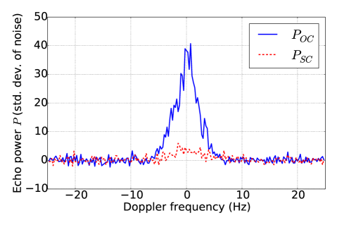
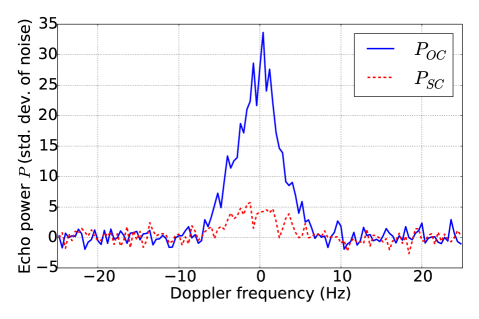
Figure 1.— Echo spectra of 1566 Icarus obtained at Arecibo on 2015 June 17 at 0.25 Hz resolution (top) and June 18 at 0.4 Hz resolution (bottom).

Table 3 Observed radar cross-sections ($\sigma$) and corresponding radar albedos ($\hat{\sigma}$) calculated on the basis of projected areas derived using our best-fit model. The Arecibo S-band $\sigma_{\rm OC,SC}$ values have uncertainties of $\sim 20\%$ due to uncertainties in the telescope gain and total power transmitted. Most of these absolute calibration errors cancel out when computing $\mu_{\rm C}$, for which we estimate uncertainties of $\sim 10\%$. One of us (SPN) calculated the Goldstone X-band $\sigma_{\rm OC,SC}$ and $\mu_{\rm C}$ values. The Goldstone $\sigma_{\rm OC,SC}$ values have uncertainties of $35\%$ due to uncertainties in telescope pointing and other calibration errors, whereas the $\mu_{\rm C}$ uncertainty is $\sim 30\%$. Latitude (lat) and longitude (lon) indicate the location of the sub-radar point, given in body-centric coordinates at the midpoint of the observation arc, with a prime meridian defined by the body’s long axis. The range of sub-radar point longitudes sampled over the duration of these observations, i.e., the rotational smear, is listed in the last column.

Date (UTC)	$\sigma_{\rm OC}$ (km2)	$\sigma_{\rm SC}$ (km2)	$\sigma_{\rm T}$ (km2)	$\mu_{\rm C}$	$\hat{\sigma}_{\rm T}$	Band	lat (deg)	lon (deg)	rot. smear (deg)
2015 Jun 13 23:40-23:58	0.1151	0.0494	0.1645	0.429	0.111	X	-40.5	258	48
2015 Jun 14 23:22-23:43	0.0599	0.0192	0.0791	0.320	0.051	X	-44.3	94	55
2015 Jun 16 23:33-01:45	0.0361	0.0115	0.0476	0.318	0.031	X	-41.3	191	348
2015 Jun 17 23:37-23:56	0.0364	0.0054	0.0418	0.149	0.028	S	-33.5	81	50
2015 Jun 18 23:23-23:36	0.0218	0.0042	0.0260	0.194	0.018	S	-25.4	267	34
2015 Jun 20 00:27-00:48	0.0201	0.0051	0.0252	0.256	0.018	S	-18.5	246	55
2015 Jun 21 00:45-01:04	0.0224	0.0031	0.0255	0.137	0.018	S	-13.5	357	50

IV.2. Bandwidth

The observed bandwidth, as measured from the CW data, reached a minimum on the second day of observations, which is consistent with the sub-radar latitude reaching an extremum on that date (Table 4) if the object is approximately spheroidal.

The predicted limb-to-limb bandwidth — which can be calculated from the expression

$$B_{LL}=\frac{4\pi D\cos{\delta}}{\lambda P},$$ (15)

where $P$ is the object’s rotational period, $\delta$ is the latitude of the sub-radar point, and $\lambda$ is the wavelength of the transmitted signal — does not appear to agree with observations. As we will discuss in detail in Section V, this object’s high specularity means that under certain observing conditions, the echo signal may contain very little power from surface regions with high incidence angles ($\theta_{inc}\gtrsim 45^{\text{$\circ$}}$), a fact already alluded to by Pettengill et al. (1969) and Goldstein (1969). As a result, the calculated limb-to-limb bandwidth does not correspond to the observed bandwidth, but the bandwidth measured at a level 1-standard-deviation above the noise does correspond to the bandwidth calculated from the shape model at the same signal strength.

Table 4A comparison of the observed bandwidths at 1-standard-deviation above the noise ($B_{>1,O}$), to that predicted by our best-fit model ($B_{>1,P}$). We attribute the discrepancy between the observed $B_{>1,O}$ and the predicted limb-to-limb bandwidth ($B_{LL}$) to the highly specular surface of 1566 Icarus, which, at low SNR, prevents the observer from receiving sufficient signal from high-incidence-angle regions. On the other hand, the $B_{>1,P}$ as predicted by the model matches the observed $B_{>1,O}$, with the exception of June 16. Bandwidth uncertainty was calculated as three times the frequency bin size. All Goldstone bandwidths have been converted into S-band Hz for ease of comparison.

	Observed	Predicted
Date (UTC)	$B_{>1,O}$ (Hz)	$B_{LL}$ (Hz)	$B_{>1,P}$ (Hz)
2015 Jun 13 23:40-23:58	10.4$\pm 1.7$	12.7	9.5
2015 Jun 14 23:22-23:43	7.8$\pm 0.4$	11.9	8.5
2015 Jun 16 23:33-01:45	12.8$\pm 0.4$	14.2	10.2
2015 Jun 17 23:37-23:56	11.8$\pm 0.8$	16.5	12.0
2015 Jun 18 23:23-23:36	13.3$\pm 1.2$	18.1	12.8
2015 Jun 20 00:27-00:48	14.2$\pm 0.8$	19.0	14.0
2015 Jun 21 00:45-01:04	14.5$\pm 4.5$	19.4	15.0

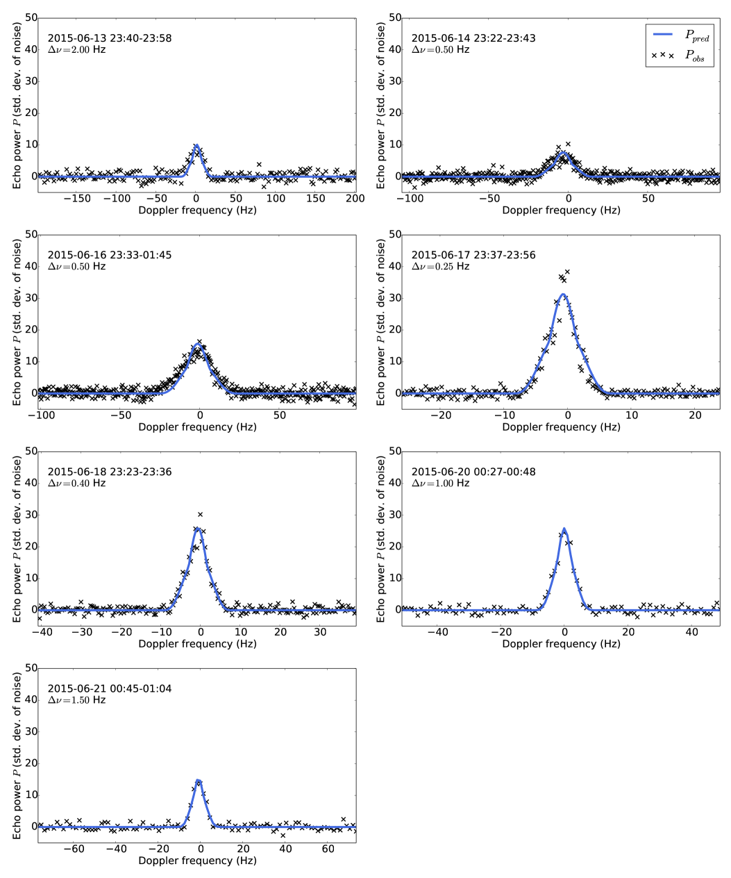
Figure 2.— Continuous-wave observations of 1566 Icarus on each day of observation. The first three sets of data were taken from Goldstone in the X-band, while the remaining four sets were taken at Arecibo in the S-band. Each set represents the summed observed powers from the corresponding day, compared to the summed predicted powers from our best-fit model. $\Delta\nu$ is the frequency resolution.

IV.3. Shape and spin pole determination

In Figure 3, we report solutions for the spin pole orientations that satisfy $\Delta\chi_{i}\leq\frac{1}{3}$ (Section III.1.2). After determining these solutions, we ran a clustering analysis based on the nearest-neighbor algorithm (Altman, 1992) to group solutions with spatially correlated spin pole positions. Figure 3 shows cluster membership with coloring. The mean three-dimensional Cartesian position of these clusters, projected onto the celestial sphere, are indicated with black crosses, and the 1- and 2-standard-deviation uncertainty regions in cluster mean position are indicated with dashed circles. Note that projection effects make these regions appear non-circular.

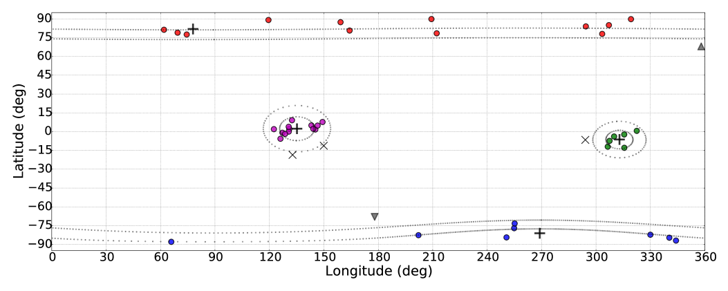
Figure 3.— Results of our search for Icarus’ spin axis orientation, in the ecliptic frame of J2000. We fit ellipsoids to the data with trial values of the spin axis orientation that were evenly distributed across the celestial sphere (Deserno, 2004) with an initial spacing of $15^{\text{$\circ$}}$. The spin pole location was allowed to float during these fits. Solutions with $\Delta\chi<\frac{1}{3}$ (Section III.1.2) were plotted as circles and colored according to cluster membership. Black crosses indicate a cluster’s mean position, whereas dotted lines show the 1- and 2-standard-deviation uncertainty region in mean cluster position. Black x’s indicate solutions that did not fall within any cluster with more than one member. Triangles show the location of the orbital poles.

Table 5 shows the two possible pairs of spin pole positions, labeled by their color (as seen in Figure 3). Each pair’s member clusters (the purple and green clusters, and the red and blue clusters) are approximate antipodes of their partner.

The associated ellipsoid axis diameters and scattering parameters (Section III.1.1) are also listed in Table 5. The uncertainty given for each parameter was calculated as the standard deviation in said parameter among members of the corresponding cluster. Because the members of each cluster are not strictly independent samples, these standard deviations may be underestimates of true uncertainties, and do not account for potential systematic errors.

Table 5Possible spin poles (ecliptic coordinates) and corresponding size and roughness values. Our adopted solution (Section V) is shown in bold, and represents a moderately flattened spheroid.

Cluster color	Spin pole		Roughness	Ellipsoid axis diameters			Equiv. diameter
	$\lambda$	$\beta$	$C$	$2a$ (km)	$2b$ (km)	$2c$ (km)	$D_{\rm eq}$ (km)
Purple	$135^{\text{$\circ$}}\pm 10^{\text{$\circ$}}$	$\;\;\;\;\;4^{\text{$\circ$}}\pm 10^{\text{$\circ$}}$	$12.9\pm 2.1$	$1.49\pm.15$	$1.53\pm.16$	$1.18\pm.13$	$1.39\pm 10\%$
Green	$313^{\text{$\circ$}}\pm 10^{\text{$\circ$}}$	$\>\;-6^{\text{$\circ$}}\pm 10^{\text{$\circ$}}$	$13.9\pm 0.7$	$1.64\pm.12$	$1.59\pm.12$	$1.18\pm.27$	$1.45\pm 13\%$
Red	$78^{\text{$\circ$}}\pm 10^{\text{$\circ$}}$	$\>\;\;82^{\text{$\circ$}}\pm 10^{\text{$\circ$}}$	$13.3\pm 2.0$	$1.65\pm.19$	$1.64\pm.19$	$1.38\pm.20$	$1.55\pm 13\%$
Blue	$\mathbf{270^{\text{$\circ$}}\pm 10^{\text{$\circ$}}}$	$\mathbf{-81^{\text{$\circ$}}\pm 10^{\text{$\circ$}}}$	$\mathbf{13.8\pm 1.4}$	$\mathbf{1.61\pm.15}$	$\mathbf{1.60\pm.17}$	$\mathbf{1.17\pm.39}$	$\mathbf{1.44\pm 18\%}$

The parameters listed in Table 5 show the specularity parameter $C$ (Equation 1) for the two pairs of spin pole solutions. All solutions are consistent with a Hagfors $C$ value of $13$. The Hagfors formalism assumes that the surface roughness has been smoothed with a wavelength-scale filter. In this formalism, the $C$ value corresponds to the root-mean-square slope ($S_{0}$) of a gently undulating surface at scales greater than the wavelength. From the expression

$$S_{0}=\frac{1}{\sqrt{C}},$$ (16)

we find that the surface of Icarus has RMS slopes of $\sim$$16^{\text{$\circ$}}$. For comparison,  Evans & Hagfors (1968) found $S_{0}$ for the lunar maria of $10.2^{\text{$\circ$}}$ and $14.8^{\text{$\circ$}}$ at wavelengths of $68$ cm and $3.6$ cm, respectively.

Figure 4 shows a series of delay-Doppler images obtained on the first day of Arecibo observations, the corresponding model images, and the residuals, while Figure 2 shows the observed Doppler spectra compared to those predicted by our adopted model. The simulated observations for this set of figures were generated from the average shape, spin pole, and scattering parameters of our adopted solution (Table 5, blue cluster).

As we will discuss in Section V, this cluster’s spin pole is our preferred solution because it is consistent with historical radar measurements and because of the sign of Icarus’ semi-major axis drift.

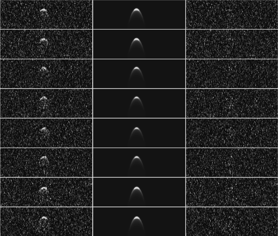
Figure 4.— Delay-Doppler images of 1566 Icarus, showing (a) the observed data, (b) simulated images from the best-fit ellipsoid model, and (c) the residual images. The delay-Doppler observations of 1566 Icarus were taken from Arecibo Observatory on June 17. These data have a range resolution of $0.2\,\mu$s, corresponding to 30 m, with four samples per baud (i.e., each pixel represents 7.5 m), and reduced with a frequency resolution of $0.30$ Hz. Each image includes $15$ looks, or independent realizations. Images are separated by $\sim$2 minutes. Within each image, range increases from top to bottom and frequency increases from left to right.

IV.4. Astrometry and orbit refinement

Our shape modeling allowed us to estimate the round-trip light times between Arecibo’s reference position and the center of mass of Icarus with a fractional precision of $\sim 10^{-8}$. We used the blue cluster shape parameters for the purpose of computing radar astrometry (Table 6).

Despite a 60+ year arc of optical observations, the inclusion of the 2015 radar astrometry reduced uncertainties on orbital parameters by a factor of $\sim$3 (Table 7).

Table 6 Arecibo radar astrometry. Round-trip light time measurements between Arecibo’s reference position and the center of mass of 1566 Icarus at the receive times listed. Estimates of the COM positions are based on fits of our best-fit shape model to the radar images.

Time (UTC)	RTT ($\mu$s)	1-$\sigma$ uncertainty ($\mu$s)
2015 Jun 18 00:02:00	58591220.06	0.4
2015 Jun 18 00:58:00	58866141.40	0.4
2015 Jun 18 23:41:00	67308377.46	1.0
2015 Jun 19 01:37:00	68163275.58	1.0
2015 Jun 20 00:58:00	79708409.31	2.0
2015 Jun 20 01:33:00	80022300.66	2.0

Table 7Orbital elements and improvements in their formal uncertainties after inclusion of the 2015 radar astrometry. The elements are semi-major axis $a$, eccentricity $e$, inclination $i$, longitude of the ascending node $\Omega$, argument of pericenter $\omega$, and mean anomaly $M$. These orbital elements are valid at the epoch 2015 June 12 00:00:00 UT with our nominal Yarkovsky drift solution (Section IV.5).

Parameter	Value	Uncertainty		Improvement factor
		Without 2015 radar data	With 2015 radar data
$a$ (au)	1.077926624685	6.5e-11	2.6e-11	2.5
$e$	0.826967321289	3.0e-08	6.9e-09	4.3
$i$ (deg)	22.828097364019	6.9e-06	2.5e-06	2.8
$\Omega$ (deg)	88.020929001348	1.6e-06	6.5e-07	2.5
$\omega$ (deg)	31.363864782557	3.4e-06	1.2e-06	2.8
$M$ (deg)	34.015936514108	1.7e-06	4.3e-07	4.0

IV.5. Yarkovsky drift

We calculated the $\hat{\alpha}$ value for Icarus’ orbit ($e=0.83$) of $\hat{\alpha}=3.16$ (Equation 8). We then identified the best-fit efficiency factor $\xi$ (Section III.4.1). Assuming a density of $\rho=2.7\text{ g}\text{ cm}^{-3}$ appropriate for Q-type asteroids (DeMeo et al., 2014) and our adopted effective diameter of $D=1.44\text{ km}$, the best-fit efficiency factor is $\xi=(4.1\pm 0.4)\%$.

The best-fit $\xi$ value corresponds to a semi-major axis drift rate of $\left\langle{da/dt}\right\rangle=(-4.62\pm 0.48)\times 10^{-4}$ au/My. This lies within one standard deviation of the value found by Nugent et al. (2012) of $\left\langle{da/dt}\right\rangle=(-3.2\pm 2.0)\times 10^{-4}$ au/My. Farnocchia et al. (2013) found a drift rate of $\left\langle{da/dt}\right\rangle=(-0.86\pm 1.8)\times 10^{-4}$ au/My. Neither of these previous results incorporated the 2015 radar astrometry, nor the more than 300 optical observations taken of 1566 Icarus since 2012.

The $p$-value (Section III.4.3) for a Yarkovsky drift model with $\left\langle{da/dt}\right\rangle=(-4.62\pm 0.48)\times 10^{-4}$ au/My and 2312 degrees of freedom is less than $10^{-10}$, leading to a confident rejection of the null hypothesis (Section III.4.3), which we interpret as a Yarkovsky detection.

In addition to conducting an analysis of variance (Table 8), we performed a variety of analyses to test the rigor of our Yarkovsky result. A description of these tests can be found in Appendix D.

Table 8 Yarkovsky measurement results for 1566 Icarus. The observational arc for these measurements was 1949–2015. The radar astrometry includes both Arecibo and Goldstone measurements from 2015. $N_{\text{opt}}$ and $N_{\text{rad}}$ indicate the number of optical (after outlier rejection) and radar measurements, respectively. $F$ indicates the F-score, which serves as a measure of significance for the necessity of a non-gravitational force component in the dynamical model (Section III.4.3). An F-score of 70 or above corresponds to a $p$-value of less than $10^{-15}$, or a detection at the $\geq 8\sigma$ level. The rows labeled MPC indicate analysis done with the full MPC data, with basic outlier rejection (which discarded 80 optical observations), and observational weighting calculated using the methods described in Farnocchia et al. (2015). The rows labeled “Screened” indicate analysis done with a smaller data set from which astrometry deemed suspect on the basis of a gravity-only model was eliminated (Jon Giorgini, pers. comm.). A full description of the data and methods used can be found in Appendix D.

Data set used	$N_{\text{opt}}$	$N_{\text{rad}}$	$\left\langle{da/dt}\right\rangle$	$F$
MPC	1148	23	$-4.6\pm 0.5$	250
	1148	-	$-4.9\pm 0.5$	264
Screened	931	23	$-4.0\pm 0.9$	139
	931	-	$-3.8\pm 1.1$	107
Screened (JLM)	931	-	$-3.6\pm 1.0$	98

We note that while our analysis of the thermal acceleration acting on Icarus assumed a spin pole aligned with the orbital pole (Section III.4.1), our final $\left\langle{da/dt}\right\rangle$ value is insensitive to this assumption. We performed numerical estimates (Figure 5) of the magnitude of the Yarkovsky effect for the four possible spin pole orientations (Section IV.3). The drift was calculated as the change in position between the best-fit Yarkovksy model and the best-fit model with no Yarkovksy effect. The $\left\langle{da/dt}\right\rangle$ value shown was calculated as the slope of a linear fit through these differences. All spin pole orientations gave consistent semi-major axis drifts. These drift rates are also consistent with the rate of $(-4.62\pm 0.48)\times 10^{-4}$ au/My, determined semi-analytically using equation (8).

We plan on using our MONTE-based orbit determination software to measure the orbital perturbations affecting other NEOs in Icarus-like orbits (Margot & Giorgini, 2010). These measurements can in turn be used to put constraints on the $\beta$ parameter in the post-Newtonian parametrization of general relativity (GR) and possibly the oblateness of the Sun. The GR and Yarkovsky perturbations are essentially orthogonal because Yarkovsky drift primarily affects the semi-major axis, whereas GR does not affect the semi-major axis but instead causes a precession of the perihelion. The cleanest separation between these perturbations will be obtained by solving for the orbits of multiple asteroids simultaneously (Margot & Giorgini, 2010).

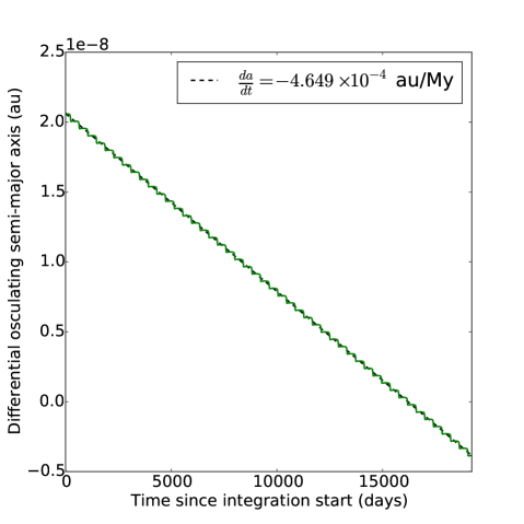
Figure 5.— The difference in semi-major axis between a $\xi=0$ Yarkovsky model and the best-fit $\xi$ value for a Yarkovsky model with spin pole located at ecliptic coordinate $\lambda=270^{\text{$\circ$}}$, $\beta=-81^{\text{$\circ$}}$, (the blue cluster). The differential semi-major axis is plotted over the time interval 1963–2015. The $\left\langle{da/dt}\right\rangle$ has been numerically estimated with a linear fit through these data. The estimated drift in semi-major axis is consistent with the result obtained when assuming a spin pole that is parallel to the orbital pole, albeit with a different value of the adjustable parameter $\xi$ (Section IV.5).

V. Discussion

V.1. Spin pole

Table 9 A comparison of measured bandwidths from previous radar observations of 1566 Icarus and bandwidths predicted for a variety of spin pole estimates. Antipodal pairs of spin poles yield bandwidths that are identical within the margin of observing error, and thus only one of each pair is shown. Table elements with an asterisk indicate a direct match between that spin pole’s bandwidth prediction and the corresponding bandwidth as reported by the authors. Bold-faced table elements indicate a match between that spin pole’s bandwidth prediction and the estimated limb-to-limb bandwidth $B_{LL}$. The $B_{LL}$ was estimated by adjusting for the decrease in apparent observed bandwidth caused by Icarus’ highly specular surface, which results in an approximate halving of the observed bandwidth as compared to the nominal limb-to-limb bandwidth for very low SNR observations. The estimated $B_{LL}$ also accounts for the fact that some authors reported the half-max bandwidth, rather than zero-crossing bandwidth. All bandwidth measurements and predictions have been converted to the Arecibo S-band frequency of 2380 MHz for ease of comparison. For observational details, see Appendix B.

Observer	Pettengill et al.		Goldstein	Mahapatra et al.	This work
Year	1968			1996	2015
Date	June 13	June 14–15	June 15–16	June 8–10	June 14	June 18	June 21
Reported by authors	${19.0}$	${4.0}$	${7.0}$	9.8	${10.4\pm 1.7}$	${11.8\pm 0.8}$	${14.5\pm 4.5}$
Estimated $B_{LL}$	37.6	12.4	17.5	19.6	12.7	16.5	19.4
This work, green (predicted)	*17.4	18.5	19.4	*12.1	14.2	16.6	19.6
This work, blue (predicted)	6.9	12.0	16.3	19.8	13.4	17.0	19.9
Gehrels et al. 1970 (predicted)	*19.9	20.0	18.9	20.0	17.7	16.3	7.8
De Angelis 1995 (predicted)	*20.1	19.3	17.5	19.1	19.5	12.9	3.4

As noted in Section IV, analysis of our radar data yields four possible sets of spin pole orientations for Icarus, and given their low $\Delta\chi$ values, these solutions are statistically indistinguishable from each other. Icarus’ spin pole has also been measured in the past from lightcurve data, which gave three possible spin poles. Lightcurve observations of Icarus between 1968 June 14 and June 21 were analyzed by Gehrels et al. (1970) and re-analyzed by De Angelis (1995). Gehrels et al. (1970) reported a spin axis orientation of $\beta=0^{\text{$\circ$}}\pm 3^{\text{$\circ$}}$, $\lambda=223^{\text{$\circ$}}\pm 3^{\text{$\circ$}}\text{ or }49^{\text{$\circ$}}\pm 3^{\text{$\circ$}}$, whereas De Angelis (1995) found $\beta=5^{\text{$\circ$}}\pm 5^{\text{$\circ$}}$, $\lambda=214^{\text{$\circ$}}\pm 5^{\text{$\circ$}}$. These lightcurve-derived spin poles are not consistent with our 2015 radar data, which leaves two possibilities – either the lightcurve-derived spin poles are incorrect, or Icarus’ spin pole has changed at some point since the 1968 apparition. We can determine which of these two possibilities is more likely by analyzing historical radar measurements of this object.

Table 9 lists Icarus’ reported bandwidths from the three radar apparitions that garnered CW measurements – namely 1968 (Pettengill et al., 1969; Goldstein, 1969), 1996 (Mahapatra et al., 1999), and 2015 (this work) – along with the bandwidths that would have been measured at the corresponding dates, if Icarus’ spin pole orientation were constant. We generated predictions for four possible spin poles – $\lambda=313^{\text{$\circ$}}\pm 10^{\text{$\circ$}},\beta=-6^{\text{$\circ$}}\pm 10^{\text{$\circ$}}$ (the green cluster), $\lambda=270^{\text{$\circ$}}\pm 10^{\text{$\circ$}},\beta=-81^{\text{$\circ$}}\pm 10^{\text{$\circ$}}$ (the blue cluster), $\beta=0^{\text{$\circ$}}\pm 3^{\text{$\circ$}},\lambda=49^{\text{$\circ$}}\pm 3^{\text{$\circ$}}$ (Gehrels et al., 1970), and $\beta=5^{\text{$\circ$}}\pm 5^{\text{$\circ$}},\lambda=214^{\text{$\circ$}}\pm 5^{\text{$\circ$}}$ (De Angelis, 1995) – and compared the predicted measurements for these poles to the reported values. A direct comparison suggests that no spin pole is consistent with measurements from more than one apparition. However, this interpretation is slightly misleading, as there were a variety of types of bandwidths reported in these articles. Pettengill et al. (1969) and  Goldstein (1969) reported bandwidths at full-width half-max (FWHM), while Mahapatra et al. (1999) reported their best estimate of the limb-to-limb bandwidth (Appendix B). In this work, we reported the measured bandwidth at one standard deviation above the noise ($B_{>1}$), as well as the limb-to-limb bandwidth calculated from our shape models. Therefore, to facilitate comparisons of these bandwidths, we have attempted to convert the historical measurements to limb-to-limb bandwidths by estimating the signal’s zero-crossing point, as well as adjusting for the decrease in apparent bandwidth caused by Icarus’ highly specular surface (Section IV.2). When comparing the predicted limb-to-limb bandwidths with these measured limb-to-limb bandwidths, we find that our red/blue cluster spin poles is consistent with all previous CW measurements of Icarus, save the first spectrum obtained by Pettengill et al. (1969) on 1968 June 13. However this measurement had a particularly low SNR, and was considered potentially problematic by the observers. Therefore, if we discard the first radar observation and assume that the lightcurve-derived spin poles are incorrect, we can find a principal axis rotation state (aligned with either the red or blue cluster solutions) that is consistent with the historical data. Furthermore, the slowly contracting orbit (Section IV.5) is indicative of a spin pole anti-aligned with the orbital pole. This suggests that, if Icarus is a principal axis rotator, it is likely to be a retrograde spinner, and thus aligned with the blue cluster solution at ecliptic coordinates

$$\lambda=270^{\text{$\circ$}}\pm 10^{\text{$\circ$}},$$

$$\beta=-81^{\text{$\circ$}}\pm 10^{\text{$\circ$}}.$$

However, if the lightcurve-derived spin poles are correct, then the spin axis orientation of Icarus would have had to have changed since the 1968 apparition. A difference in spin orientation may be caused by non-principal axis (NPA) rotation or the effect of torques due to anisotropic mass loss. Mass loss may occur due to thermal fracturing. NPA rotation may remain undetected in lightcurve or radar data if one of the fundamental periods is long compared to the span of observations in any given apparition or if the object is approximately spheroidal. NPA rotation requires a mechanism to excite the spin state on a time scale shorter than the NPA damping time scale. The Burns & Safronov (1973) time scale for damping to principal axis rotation assuming silicate rock ($\mu Q$ = 5 $\times 10^{12}$ Nm^-2, $\rho=2.71\text{ g}\text{ cm}^{-3}$) is $\sim$25 million years, during which Icarus experiences close planetary encounters that may excite its spin. However, if the material properties are closer to those reported by Scheirich et al. (2015) ($\mu Q$ = 1.3 $\times 10^{7}$ Nm^-2), NPA rotation would require an excitation in the past 100 years, which we consider unlikely.

Three arguments favor the principal axis rotation solution: (1) the lightcurve-derived spin poles predict bandwidths that are inconsistent with observations (Table 9), (2) the bandwidths predicted by the blue cluster spin pole solutions can match observations over three separate apparitions, (3) damping to principal axis rotation would likely occur on short time scales. This conclusion suggests that interpreting the evolution of lightcurve amplitudes may not be sufficient in determining spin pole orientations accurately. Other considerations, such as knowledge of albedo variations and inhomogeneous scattering behavior, may be necessary to properly interpret lightcurve data.

V.2. Cross-section and size

Using the results of our analysis, we have found that 1566 Icarus’ radar scattering behavior is consistent with a Hagfors specularity constant of $C=13$. This level of specularity is unusual for NEOs (Appendix C), and helps to explain the lower-than-expected image quality. Diffusely-scattering surfaces can reflect power from high incidence angles – therefore, surface elements with normal vectors not aligned with the observer’s line of sight can still contribute to the return signal. The surface elements of specular objects, on the other hand, reflect most of their incident power away from the observer unless they lie close to the sub-radar point (for ellipsoidal objects). The result is a very sharp drop-off in SNR for incidence angles greater than $\sim$$20^{\text{$\circ$}}$. This effect can be seen in Figure 4.

Furthermore, the small amount of echo power returning from regions with high incidence angles ($\theta_{inc}\gtrsim 45^{\text{$\circ$}}$) helps to resolve the difference between Icarus’ observed bandwidth and the limb-to-limb bandwidth calculated from the object’s shape and spin pole orientation (Table 4). The most highly red- and blue- shifted signals are reflected from these high-incidence regions, and the large attenuation of these signals reduces the span of the measured bandwidth. This effect may also explain a discrepancy noticed by Mahapatra et al. (1999), who measured Icarus’ bandwidth during its previous radar apparition nearly two decades ago, and pointed out that the measured bandwidth corresponds to a diameter around half of the value found radiometrically by Harris (1998).

The results presented within this work suggest Icarus’ surface and sub-surface properties are unusual amongst the known population of NEOs. The radar albedo $\hat{\sigma}_{T}$ (defined as the radar cross-section divided by the object’s geometric cross-section) for an object with a diameter of $\sim$$1.44$ km and a measured radar cross-section of $0.03\text{ km}^{2}$ is less than 2% (see Table 3), which we believe to be the lowest radar albedo ever measured (e.g., Magri et al., 1999, 2001, 2007a).

The radar albedo for a specular reflector provides an approximation to the Fresnel reflectivity, which is related to the dielectric constant (Evans & Hagfors, 1968). Our radar albedo measurement yields the surprising low dielectric constant of 1.8. Most non-volcanic rocks have dielectric constants above 5, unless they are in a powdered form with high porosity (Campbell & Ulrichs, 1969), in which case their dielectric constants are about 2. Our measurements suggest that Icarus may have a low surface density or, equivalently, a high surface porosity.

Furthermore, a radar specularity of $C=13$ is unusually high compared to most radar-imaged NEOs. This high specularity and low radar albedo suggest an unusual surface structure. Due to its highly eccentric orbit ($e=0.82$) and low semi-major axis ($a=1.08$ au), Icarus approaches within $0.19$ au of the Sun. At that distance, the equilibrium sub-solar point temperature is expected to lie between $600$ K and $900$ K.  Jewitt & Li (2010) found that at temperatures within this range, certain mineral compounds undergo extensive structural changes, possibly through the mechanism of thermal fatigue (Delbo et al., 2014). It is possible that a combination of cratering history, spin evolution, and repeated close approaches to the sun have modified the surface of Icarus in such a way as to substantially lower its radar albedo.

Finally, we point out that the equivalent diameter determined herein adds to the list of conflicting sizes estimates for Icarus in the literature. Using various thermal models, Harris (1998) found a diameter of anywhere between $0.88$ km and $1.27$ km. Mainzer et al. (2012) determined a diameter of $1.36\pm 0.43$ km using NEOWISE data at $3.4\mu$m, $4.6\mu$m, and $12\mu$m, and the Near-Earth Asteroid Model (NEATM) (Harris, 1998). Following their 1999 CW measurements of Icarus, Mahapatra et al. (1999) calculated a diameter between $0.6-0.8$ km, assuming the spin pole reported by De Angelis (1995). Finally, a diameter can be calculated from the expression (Fowler & Chillemi, 1992)

$$D=\frac{10^{-0.2H}1329}{\sqrt{p_{V}}},$$ (17)

which, coupled with the measured H-magnitude of $16.3$ (Harris, 1998) and geometric albedo $p_{V}$ of 0.14 (Thomas et al., 2011), yields a diameter of $1.95$ km. More recent lightcurve measurements obtained at large phase angles yield $H=15.5$ (Warner, 2015), which corresponds to a diameter of $2.80$ km. We found an equivalent diameter of 1.44 km with 18% uncertainties.

VI. Conclusions

In this work, we analyzed Arecibo and Goldstone radar observations of 1566 Icarus to estimate its size, shape, scattering properties, orbital parameters, and Yarkovsky drift. These results suggest that this object has unusual surface properties, and resolves long-standing questions about the object’s size.

We presented the first use of our orbit-determination software and demonstrated its ability to generate accurate radar ephemerides and to determine the magnitude of subtle accelerations such as the Yarkovsky effect.

Appendix A A. Yarkovsky acceleration

For an object with diameter $D$, at distance from the Sun at time $t$ of $r_{t}$, the energy absorbed per second is

$$\dot{E}=\frac{L_{\odot}}{4\pi r_{t}^{2}}\;\pi\left(\frac{D}{2}\right)^{2},$$

assuming perfect absorption.

The acceleration $\ddot{r}$ is equal to the photon momentum absorbed, $\dot{p_{\gamma}}$, over the mass of the object, $m$.

$$\ddot{r} =\frac{\dot{p_{\gamma}}}{m}$$

$$=\frac{\dot{E}/c}{m}$$

$$=\frac{L_{\odot}}{4\pi r_{t}^{2}}\;\pi\left(\frac{D}{2}\right)^{2}\;\frac{1}{c}\;\frac{1}{m}.$$

Expressing the object mass in terms of density, $\rho$, and $D$, yields

$$\ddot{r} =\frac{L_{\odot}}{4\pi r_{t}^{2}}\;\pi\left(\frac{D}{2}\right)^{2}\;\frac{1}{c}\;\frac{1}{\frac{4}{3}\pi\left(\frac{D}{2}\right)^{3}\rho}$$

$$=\frac{3}{8\pi}\;\frac{L_{\odot}}{c}\;\frac{1}{r_{t}^{2}}\;\frac{1}{D\rho}.$$

This acceleration is applied in the positive radial direction (in heliocentric coordinates).

$$\ddot{\vec{r}}=\frac{3}{8\pi}\;\frac{1}{D\rho}\;\frac{L_{\odot}}{c}\;\frac{1}{r_{t}^{2}}\;\hat{r}$$

Because it is purely radial, this acceleration will not cause a measurable change in the orbit.

However, the absorbed photons will eventually be re-radiated, and induce an acceleration upon emission as well. Since the object is rotating about some spin axis $\hat{p}$, this secondary acceleration will not (necessarily) occur along a radial direction. Furthermore, given that all the absorbed photons must eventually be re-radiated, we can express the magnitude of this secondary acceleration in the same manner as its radial counterpart. Here we define a phase lag, $\phi$, to describe at what rotational phase (relative to the sub-solar longitude) the majority of the photons are re-emitted, and an efficiency factor, $\xi$, which is tied to the effective acceleration if one assumes that all photons are re-emitted with phase lag $\phi$. $X_{\hat{p}}(\phi)$ is the rotation matrix of angle $\phi$ about $\hat{p}$.

$$\ddot{\vec{r}}=\xi\;\frac{3}{8\pi}\;\frac{1}{D\rho}\;\frac{L_{\odot}}{c}\;\frac{X_{\hat{p}}(\phi)\vec{r_{t}}}{||\vec{r_{t}}||^{3}}.$$

The Yarkovsky effect is caused by this non-radial secondary acceleration.

Appendix B B. Historical data concerning 1566 Icarus’ spin pole orientation

For the purpose of facilitating bandwidth comparisons, we normalize all bandwidths to the Arecibo S-band frequency of 2380 MHz and label the corresponding unit S-Hz. Except where otherwise noted, the bandwidths discussed here are relayed as they were reported in the corresponding articles – i.e., without any corrections applied for specularity. We also note the distinction between reported half-power bandwidths and zero-crossing bandwidths.

B.1. Pettengill et al. 1968 radar observations

The radar detection of Icarus by Pettengill et al. (1969) on 1968 June 13 marked the first detection of an asteroid with radar. These observations were conducted at the Haystack Observatory at a frequency of 7840 MHz. A second set of observations took place on 1968 June 15. Pettengill et al. (1969) observed half-power Doppler extents of 70 Hz on June 13 and 13 Hz on June 15. Because both sets of observations spanned multiple rotations of Icarus, the change in bandwidth cannot be attributed to the shape of the object.

The bandwidth reported on June 13 is over-estimated, for two reasons. First, the authors reported a drift of their data-taking ephemeris by 8 Hz over the data-taking period, indicating that the echo was at most 62 Hz. Second, the authors applied a variety of smoothing windows (8, 16, 32, and 64 Hz) and reported only the spectrum with the maximum signal-to-noise ratio, which they obtained with the 64 Hz smoothing window. Because the convolution operation broadened the echo, we estimate that the original, intrinsic echo was between 32 and 62 Hz.

Thus, the June 13 Pettengill et al. (1969) half-power bandwidth correspond to a value between 9.7 S-Hz and 19 S-Hz, and the June 15 bandwidth corresponds to 4.0 S-Hz.

B.2. Goldstein 1968 radar observations

Goldstein (1969) detected Icarus between 1968 June 14 and 16 with a bistatic configuration at Goldstone. The frequency was 2388 MHz and the reported half-power bandwidth for observations between June 15 04:30 UT and June 16 10:00 UT is about 7 Hz (or 7 S-Hz).

B.3. Gehrels et al. 1968 lightcurve observations

Lightcurve observations of Icarus between 1968 June 14 and June 21 were analyzed by Gehrels et al. (1970) and re-analyzed by De Angelis (1995). Gehrels et al. (1970) reported a spin axis orientation of $\beta=0^{\text{$\circ$}}\pm 3^{\text{$\circ$}}$, $\lambda=223^{\text{$\circ$}}\pm 3^{\text{$\circ$}}\text{ or }49^{\text{$\circ$}}\pm 3^{\text{$\circ$}}$, whereas De Angelis (1995) found $\beta=5^{\text{$\circ$}}\pm 5^{\text{$\circ$}}$, $\lambda=214^{\text{$\circ$}}\pm 5^{\text{$\circ$}}$. These spin poles do not appear to be consistent with most of the radar CW bandwidths observed during the 1968, 1996, or 2015 apparitions (Table 9).

B.4. Mahapatra et al. 1996 radar observations

Mahapatra et al. (1999) used Goldstone and observed a zero-crossing Doppler bandwidth of 35 Hz at 8510 MHz. Because they used a 10 Hz smoothing window, the intrinsic bandwidth could be 35–45 Hz, or a value between 9.8 and 12.6 S-Hz.

Appendix C C. Attempts to fit a lower specularity

The specularity reported in this work for 1566 Icarus is unusually high. When originally fitting the shape and scattering properties for this object, we initially forced a lower specularity on our models. After many such attempts, we came to the conclusion that a diffusely-scattering surface did not match the data we observed.

Figure 6 demonstrates what an attempted fit to Icarus’ CW spectra and delay-Doppler images looks like, when the specularity is fixed to a lower value of $C=2$, and a ‘cos’ scattering law is utilized. This scattering behavior can be defined with respect to the differential radar cross section per surface element area (Section III.1.1), via

$$\frac{d\sigma}{dA}=R(C+1)\cos^{2C}{\theta}.$$ (C1)

These fits are the result of allowing all other model parameters (ellipsoid axis ratios, signal scaling parameters, etc.) to float, and performing a full fit on the same dataset used for the results reported in this article. The best-fit model has an equivalent diameter of $1.05$ km and, as the figure demonstrates, results in a poor fit to the data. Note in particular that while the bounds of the model spectrum is approximately equal to the bounds of the data spectrum, the shape of the spectra do not match. In addition, the signal in the delay-Doppler image does not drop off fast enough as range from the observer increases. The fast drop-off noted in the data necessitates a specular model. Such a model can be realized with either a two-component ‘cos’ scattering law or a ‘hagfors’ scattering law.

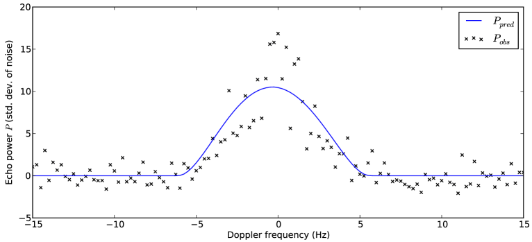
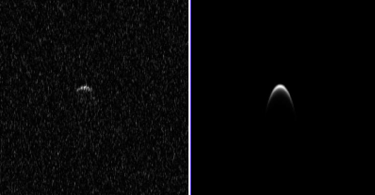
Figure 6.— A result of a global fit to CW spectra and delay-Doppler images of 1566 Icarus, with the specularity constant $C$ fixed to $2.0$. Shown is an example comparison between the observed data and best-fit model spectrum for data taken on June 17, (top), as well as a comparison between a best-fit model delay-Doppler image (bottom right) and the corresponding observed image (bottom left), also taken on June 17. The fit shown does not match the data, and suggests that a higher specularity model is needed.

Appendix D D. Additional evidence of Yarkovsky detection

We performed a variety of analyses to test the rigor of our Yarkovsky result (Section IV.5).

D.1. Screening test

We re-ran our Yarkovsky analysis with an independently curated set of optical and radar astrometry (Jon Giorgini, pers. comm.). This data set has been screened for potential outliers and faulty measurements using a gravity-only model, with around 20% of the original astrometric data being discarded. Our analysis of these data (931 optical astrometric points and 23 radar astrometric points from 1949 to 2015) yielded a drift in semi-major axis of $\left\langle{da/dt}\right\rangle=-4.0\pm 0.9\times 10^{-4}$ au/My when including both radar and optical astrometry and $\left\langle{da/dt}\right\rangle=-3.8\pm 1.1\times 10^{-4}$ au/My when including optical astrometry only (Table 8).

As a further verification, one of us (JLM) used the software he developed in previous work (Nugent et al., 2012) with this independently screened data set and found $\left\langle{da/dt}\right\rangle=(-3.6\pm 1.0)\times 10^{-4}$ au/My (Table 8).

D.2. Prediction test

One way to analyze the accuracy of a Yarkovsky result is to check its predictive power when compared to a gravity-only dynamical model. Instead of collecting additional astrometry, which is not straightforward, we can simulate a prediction by re-analyzing a subset of the data before some fiducial point in time, $t_{f}$, and then checking how the resulting trajectory fares at predicting observations that were taken after $t_{f}$.

The first range measurement of Icarus was obtained from Goldstone on June 14, 2015 (Table 2). We therefore chose 2015-June-13 23:50 UT as $t_{f}$. We fit a Yarkovsky model to the data taken before $t_{f}$ (936 optical observations and 11 radar observations, from which 55 optical observations were discarded as outliers), and found a semi-major axis drift rate of $\left\langle{da/dt}\right\rangle=(-3.7\pm 0.7)\times 10^{-4}$ au/My. This fit yielded a goodness-of-fit of $\chi^{2}=634$. We also fit a gravity-only model to the same set of data, which resulted in a goodness-of-fit of $\chi^{2}=662$. We then compared how well these best-fit trajectories could predict the first Icarus range measurement on June 14, 2015. The best-fit Yarkovsky model residual for this prediction was 97 km, while the best-fit gravity-only model residual was 267 km. This demonstrates that the Yarkovsky model more accurately predicted a future measurement than the gravity-only model.

D.3. Incorporation test

Another test of rigor is an incorporation test. After performing the prediction test described above, we then added the first Doppler and range measurements of 2015 and fit both a gravity-only model and a Yarkovsky model once again. No additional outlier rejection was allowed. With these new Doppler and range measurements, the best-fit semi-major axis drift rate for the Yarkovsky model is $\left\langle{da/dt}\right\rangle=(-4.7\pm 0.5)\times 10^{-4}$ au/My. The goodness-of-fit for the Yarkovsky model is $\chi^{2}=638$, or a $<1$% increase as compared to the Yarkovsky fit prior to including the new radar measurements. The best-fit gravity-only model yielded a goodness-of-fit of $\chi^{2}=719$, or a 9% increase as compared to the gravity-only fit prior to including the new radar measurements. These results suggest that incorporating the first Icarus radar measurements into a gravity-only model results in a general degradation in the quality of the fit to optical observations. However, these same radar measurements can be included in a Yarkovsky model with no appreciable effect on the goodness-of-fit.

D.4. Combined test

Finally, we re-ran both the prediction test and the incorporation test described above on the curated data set. The best-fit Yarkovsky model fit to data taken before $t_{f}$ yielded a drift in semi-major axis of $\left\langle{da/dt}\right\rangle=(-3.53\pm 1.11)\times 10^{-4}$ au/My, and a goodness-of-fit of $\chi^{2}=172$, while the gravity-only model had a goodness-of-fit of $\chi^{2}=182$. The Yarkovsky model predicted the first Goldstone range measurement with a residual of 43 km, while the gravity-only model predicted residual for that data point was 128 km. For the incorporation test, we again added the first Goldstone Doppler and range measurements to the data set. For the Yarkovsky model, the best-fit drift in semi-major axis was $\left\langle{da/dt}\right\rangle=(-3.95\pm 0.97)\times 10^{-4}$ au/My, with a goodness-of-fit of $\chi^{2}=173$, or an increase of $<1$% as compared to the Yarkovsky fit prior to adding the new radar measurements. The best-fit gravity-only model had a goodness-of-fit of $\chi^{2}=189$, or a $4$% increase as compared to the gravity-only model fit prior to adding the new radar measurements. Note that these fits were performed on a data set for which outlier rejection had been performed assuming a gravity-only model — even so, a gravity-only model still required a marked decrease in fit quality in order to incorporate the first radar measurements, while the Yarkovsky model saw no appreciable change in goodness-of-fit.

D.5. Summary

The tests that we performed are summarized in Table 10 and Table 11, and confirm the robustness of the Yarkovsky detection.

Table 10 The residuals of the first range measurement obtained of 1566 Icarus when using a Yarkovsky model and a gravity-only model, and when fitting these models only to data taken before the first radar measurements of 2015 (i.e., the prediction test).

	Residual (km)
Data set	Yarkovsky model	Gravity-only model
MPC	97	267
Screened	43	128

Table 11 The goodness-of-fit ($\chi^{2}$) for a Yarkovsky model and a gravity-only model when fit to only data taken before the first radar measurements of 2015 (i.e., before $t_{f}=$ 2015-June-13 23:50:00 UT), and how $\chi^{2}$ changes when the first Doppler and range measurements are incorporated into the fit (i.e., the incorporation test).

MPC data set
	Yarkovsky model	Gravity-only model
All data prior to $t_{f}$	634	661
All data prior to $t_{f}$ + 1 range, 1 Doppler	638	719
Fractional increase in $\chi^{2}$	$<1$%	9%
Screened data set
	Yarkovsky model	Gravity-only model
All data prior to $t_{f}$	172	182
All data prior to $t_{f}$ + 1 range, 1 Doppler	173	189
Fractional increase in $\chi^{2}$	$<1$%	4%

References

- Altman (1992) Altman, N. S. 1992, The American Statistician, 46, 175
- Bierman (1977) Bierman, G. J. 1977, ”Factorization Methods for Discrete Sequential Estimation” (Dover)
- Burns (1976) Burns, J. A. 1976, American Journal of Physics, 44, 944
- Burns & Safronov (1973) Burns, J. A., & Safronov, V. S. 1973, MNRAS, 165, 403
- Campbell & Ulrichs (1969) Campbell, M. J., & Ulrichs, J. 1969, J. Geophys. Res., 74, 5867
- De Angelis (1995) De Angelis, G. 1995, Planet. Space Sci., 43, 649
- Delbo et al. (2014) Delbo, M., Libourel, G., Wilkerson, J., et al. 2014, Nature, 508, 233
- DeMeo et al. (2014) DeMeo, F. E., Binzel, R. P., & Lockhart, M. 2014, Icarus, 227, 112
- Deserno (2004) Deserno, M. 2004, How to generate equidistributed points on the surface of a sphere, https://www.cmu.edu/biolphys/deserno/pdf/sphere_equi.pdf
- Evans & Hagfors (1968) Evans, J. V., & Hagfors, T., eds. 1968, Radar Astronomy (New York: McGraw-Hill)
- Evans et al. (2016) Evans, S., Taber, W., Drain, T., et al. 2016, in The 6th International Conference on Astrodynamics Tools and Techniques (ICATT), International Conference on Astrodynamics Tools and Techniques, Darmstadt, Germany
- Farnocchia et al. (2015) Farnocchia, D., Chesley, S., Chamberlin, A., & Tholen, D. 2015, Icarus, 245, 94
- Farnocchia et al. (2013) Farnocchia, D., Chesley, S. R., Vokrouhlický, D., et al. 2013, Icarus, 224, 1
- Folkner et al. (2014) Folkner, W. M., Williams, J. G., Boggs, D. H., Park, R. S., & Kuchynka, P. 2014, Interplanetary Network Progress Report, 196, 1
- Fowler & Chillemi (1992) Fowler, J. W., & Chillemi, J. R. 1992, The IRAS Minor Planet Survey, 17
- Gehrels et al. (1970) Gehrels, T., Roemer, E., Taylor, R. C., & Zellner, B. H. 1970, AJ, 75, 186
- Giorgini et al. (2002) Giorgini, J. D., Ostro, S. J., Benner, L. A. M., et al. 2002, Science, 296, 132
- Goldstein (1969) Goldstein, R. M. 1969, Icarus, 10, 430
- Greenberg & Margot (2015) Greenberg, A. H., & Margot, J.-L. 2015, AJ, 150, 114
- Hagfors (1964) Hagfors, T. 1964, J. Geophys. Res., 69, 3779
- Harris (1998) Harris, A. W. 1998, Icarus, 131, 291
- Hudson & Ostro (1994) Hudson, R. S., & Ostro, S. J. 1994, Science, 263, 940
- Jewitt & Li (2010) Jewitt, D., & Li, J. 2010, AJ, 140, 1519
- Kalman (1960) Kalman, R. E. 1960, Transactions of the ASME–Journal of Basic Engineering, 82, 35
- Magri et al. (2001) Magri, C., Consolmagno, G. J., Ostro, S. J., Benner, L. A. M., & Beeney, B. R. 2001, Meteoritics and Planetary Science, 36, 1697
- Magri et al. (2007a) Magri, C., Nolan, M. C., Ostro, S. J., & Giorgini, J. D. 2007a, Icarus, 186, 126
- Magri et al. (2007b) Magri, C., Ostro, S. J., Scheeres, D. J., et al. 2007b, Icarus, 186, 152
- Magri et al. (1999) Magri, C., Ostro, S., Rosema, K., et al. 1999, Icarus, 140, 379
- Mahapatra et al. (1999) Mahapatra, P. R., Ostro, S. J., Benner, L. A. M., et al. 1999, Planet. Space Sci., 47, 987
- Mainzer et al. (2012) Mainzer, A., Grav, T., Masiero, J., et al. 2012, ApJ, 760, L12
- Mandel (1964) Mandel, J. 1964, The Statistical Analysis of Experimental Data (Dover Publications)
- Margot & Giorgini (2010) Margot, J. L., & Giorgini, J. D. 2010, in IAU Symposium, Vol. 261, IAU Symposium, ed. S. A. Klioner, P. K. Seidelmann, & M. H. Soffel, 183–188
- Minor Planet Center (2015) Minor Planet Center. 2015, Minor Planet database, http://minorplanetcenter.net/db_search
- Nugent et al. (2012) Nugent, C. R., Margot, J. L., Chesley, S. R., & Vokrouhlický, D. 2012, Astronomical Journal, 144, 60
- Ostro (1993) Ostro, S. J. 1993, Reviews of Modern Physics, 65, 1235
- Peterson (1976) Peterson, C. A. 1976, PhD thesis, Massachusetts Institute of Technology.
- Pettengill et al. (1969) Pettengill, G. H., Shapiro, I. I., Ash, M. E., et al. 1969, Icarus, 10, 432
- Press et al. (1992) Press, W. H., Teukolsky, S. A., Vetterling, W. T., & Flannery, B. P. 1992, Numerical Recipes in C (2nd Ed.): The Art of Scientific Computing (New York, NY, USA: Cambridge University Press)
- Rubincam (2000) Rubincam, D. P. 2000, Icarus, 148, 2
- Scheirich et al. (2015) Scheirich, P., Pravec, P., Jacobson, S. A., et al. 2015, Icarus, 245, 56
- Thomas et al. (2011) Thomas, C. A., Trilling, D. E., Emery, J. P., et al. 2011, AJ, 142, 85
- Verma & Margot (2016) Verma, A. K., & Margot, J. L. 2016, JGR
- Vokrouhlický & Farinella (1998) Vokrouhlický, D., & Farinella, P. 1998, AJ, 116, 2032
- Vokrouhlický et al. (2000) Vokrouhlický, D., Milani, A., & Chesley, S. R. 2000, Icarus, 148, 118
- Warner (2015) Warner, B. D. 2015, Minor Planet Bulletin, Vol. 42, http://www.minorplanet.info/MPB/MPB_424.pdf