Reductions of Binary Trees and Lattice Paths
induced by the Register Function

Abstract.

The register function (or Horton-Strahler number) of a binary tree is a well-known combinatorial parameter. We study a reduction procedure for binary trees which offers a new interpretation for the register function as the maximal number of reductions that can be applied to a given tree. In particular, the precise asymptotic behavior of the number of certain substructures (“branches”) that occur when reducing a tree repeatedly is determined.

In the same manner we introduce a reduction for simple two-dimensional lattice paths from which a complexity measure similar to the register function can be derived. We analyze this quantity, as well as the (cumulative) size of an (iteratively) reduced lattice path asymptotically.

1. Introduction

The aim of this paper is to investigate local substructures that appear within discrete objects after reducing according to, in some sense, intrinsic rules. In particular, there are two reductions we focus on: a reduction for binary trees, as well as a reduction for simple two-dimensional lattice paths.

In order to give a summary of our results we will briefly sketch both reductions and explain the nature of the local structures emerging when applying the reduction repeatedly.

On a general note, we made heavy use of the open-source mathematics software system SageMath [1] in order to perform the computationally intensive parts of the asymptotic analysis for all of the parameters investigated in this paper. Files containing these computations as well as instructions on how to run them with SageMath can be found at https://benjamin-hackl.at/publications/register-reduction/.

1.1. Binary Trees

Binary trees are either a leaf or a root together with a left and a right subtree which are binary trees. This recursive definition can be written as a symbolic equation ($\square$ and mark leaves and inner nodes, respectively):

By using the symbolic method (cf. [10, Part A]), this equation can be translated into a functional equation for the generating function counting binary trees with respect to their size (i.e. the number of inner nodes). The corresponding functional equation is given by

$$B(z)=1+zB(z)^{2},$$

which leads to the well-known expansion

$$B(z)=\frac{1-\sqrt{1-4z}}{2z}=\sum_{n\geq 0}\frac{1}{n+1}\binom{2n}{n}z^{n}.$$

This means that the number of binary trees with $n$ inner nodes is given by the $n$th Catalan number $C_{n}=\frac{1}{n+1}\binom{2n}{n}$.

By simple algebraic manipulations, it is easy to verify that the generating function $B(z)$ satisfies the identity

$$B(z)=1+\frac{z}{1-2z}B\Big{(}\frac{z^{2}}{(1-2z)^{2}}\Big{)}.$$

However, as we will see in Section 2, we can justify this identity from a combinatorial point of view as well, and the most important part of this combinatorial interpretation is a reduction procedure for binary trees.

Essentially, this procedure first removes all leaves from the tree and then “repairs” the resulting object by collapsing chains of nodes with only one child into one node. More details on this reduction are provided in Section 2.

With the help of this reduction we can assign labels to all nodes in a given tree by tracking how many iterated tree reductions it takes until the node is deleted. Note that collapsing some nodes into one node does not count as deleting the node. In Section 2 we prove that these labels are intimately linked with a very well-known and well-studied branching complexity measure of binary trees: the register function.

The local structures we are interested in also become visible after labeling a tree as described above: the so-called $r$-branches of a binary tree are the connected subgraphs of nodes with label $r$. The number of these $r$-branches in a random tree of size $n$ is modeled by the random variable $X_{n;r}\colon\mathscr{B}_{n}\to\mathbb{N}_{0}$, where $\mathscr{B}_{n}$ is the set of all binary trees of size $n$. A proper definition as well as results on $r$-branches can be found in Section 2.2.

In the context of binary tree reductions we are interested in precise analyses of the random variables $X_{n;r}$ as well as $X_{n}:=\sum_{r\geq 0}X_{n;r}$, which models the total number of branches in a random tree of size $n$. This quantity is investigated closely in Section 2.3.

Table 1 gives an overview of the results of our investigation. The results for the register function are well-known, which is why we refer to external literature instead. Additionally, Theorem 2 proves asymptotic normality for the number of $r$-branches $X_{n;r}$.

	Register function	$r$-branches ($X_{n;r}$)	branches total ($X_{n}$)
range	[9, Sec. 1.1, Sec 2]	Proposition 2.5	Proposition 2.7
explicit formula	[9, Theorem 1]	Proposition 2.6	Proposition 2.8
asymptotic formula	[9, Theorem 3]	Theorem 1	Theorem 3

Table 1. Results: binary trees

1.2. Lattice Paths

Let $\mathscr{L}$ be the combinatorial class of simple two-dimensional lattice paths, i.e., the set of all nonempty sequences over $\{\mathnormal{\uparrow},\mathnormal{\rightarrow},\mathnormal{\downarrow},\mathnormal{\leftarrow}\}$. It is easy to see that the corresponding generating function is

$$L(z)=\frac{4z}{1-4z}.$$

Similarly to before, it is easy to check by algebraic manipulation that $L(z)$ satisfies the functional equation

$$L(z)=4L\Big{(}\frac{z^{2}}{(1-2z)^{2}}\Big{)}+4z.$$

However, as in the case of binary trees, we will see in Section 3 that the combinatorial interpretation of this equation is much more fruitful and gives rise to a reduction procedure for lattice paths.

In this case it takes a bit more to fully describe the reduction. The core idea is to reduce a given path by collapsing an entire horizontal-vertical segment (i.e. a path segment that consists of a sequence of horizontal movements followed by a sequence of vertical movements) into a single step.

The first parameter of interest in this context is the reduction degree of a random path of length $n$, which is the number of repeated reductions that it takes until the entire path is reduced to a single step. We will model this parameter with the random variable $D_{n}\colon\mathscr{L}_{n}\to\mathbb{N}_{0}$, where $\mathscr{L}_{n}$ consists of all simple two-dimensional lattice paths of length $n$.

As an analogue to the number of $r$-branches in a given binary tree we consider the length of the $r$th fringe, i.e., the $r$th reduction of a given lattice path. This quantity is modeled by the random variable $X_{n;r}^{L}\colon\mathscr{L}\to\mathbb{N}_{0}$.

By summation of the length of the $r$th fringe for $r\geq 0$ we obtain the total fringe size $X_{n}^{L}:=\sum_{r\geq 0}X_{n;r}^{L}$. In some sense, the total fringe size measures the complexity of horizontal-vertical direction changes of a given lattice path. Both, the $r$th fringe size as well as the total fringe size are analyzed in Section 3.2.

Table 2 gives an overview of the results of our investigation.

	Reduction degree ($D_{n}$)	$r$-fringes ($X_{n;r}^{L}$)	total fringe size ($X_{n}^{L}$)
range	Proposition 3.5	Proposition 3.7	Proposition 3.9
explicit formula	Corollary 3.4	Proposition 3.8	Corollary 3.10
asymptotic formula	Theorem 4	Theorem 5	Theorem 6

Table 2. Results: lattice paths

2. Tree Reductions and the Register Function

2.1. Motivation and Preliminaries

As mentioned in the introduction, we want to find a combinatorial proof of the following proposition.

Proposition 2.1.

The generating function counting binary trees by the number of inner nodes, $B(z)=\frac{1-\sqrt{1-4z}}{2z}$, satisfies the identity

$$B(z)=1+\frac{z}{1-2z}B\Big{(}\frac{z^{2}}{(1-2z)^{2}}\Big{)}.$$ (1)

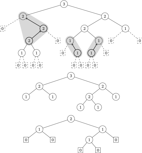
Figure 1. Illustration of the tree reduction $\Phi$: in the first tree, the leaves are deleted (dashed nodes) and nodes with exactly one child are merged (gray overlay). The second tree shows the result of these operations. Finally, in the last tree all nodes without children are marked as leaves.

Proof.

We consider the following reduction of a binary tree $t$, which we write as $\Phi(t)$:

First, all leaves of $t$ are erased. Then, if a node has only one child, these two nodes are merged; this operation will be repeated as long as there are such nodes. The leaves of the reduced tree are precisely the nodes without children.

This operation was introduced in [32]. The various steps of the reduction are depicted in Figure 1. The numbers attached to the nodes will be explained later.

Note that $\Phi(\square)$ is undefined, so this is a partial function. Of course, many different trees are mapped to the same binary tree. However, they can all be obtained from a given reduced tree by the following operations:

All leaves and all internal nodes in the tree are replaced by chains of internal nodes. In such a chain, there has to be at least one leaf attached to every internal node; the symbolic equation for chains is

Obviously, these substitutions do not only restore the (previously deleted) leaves, but can also “unmerge” previously merged nodes. Thus, all trees that reduce to some tree $t^{\prime}$ can be reconstructed from $t^{\prime}$.

From the symbolic equation of chains above, we find that the generating function $C(z)$ counting chains with respect to their size (i.e. number of internal nodes) satisfies the equation $C(z)=z+2zC(z)$ and thus, we obtain

$$C(z)=\frac{z}{1-2z}.$$

Finally, if $F(z)$ is a generating function counting some family of binary trees, then the bivariate generating function $vF(zv)$ counts the same family with respect to size (variable $z$) and number of leaves (variable $v$). This is a direct consequence of the fact that binary trees with $n$ inner nodes have $n+1$ leaves.

Therefore, replacing all nodes of a binary tree with chains corresponds to the substitutions $v\mapsto\frac{z}{1-2z}$ and $z\mapsto\frac{z}{1-2z}$ in the language of generating functions. Therefore, all binary trees that can be reconstructed from a reduced version of itself are counted by

$$\frac{z}{1-2z}B\Big{(}\frac{z^{2}}{(1-2z)^{2}}\Big{)}.$$

By all these considerations, (1) can be interpreted combinatorially as the following statement: a binary tree is either just $\square$, or it can be reconstructed from another binary tree where all nodes are replaced by chains. ∎

Remark.

Note that (1) can be used to find a very simple proof for a well-known identity for Catalan numbers:

Comparing the coefficients of $z^{n+1}$, (1) leads to

$$C_{n+1} =[z^{n+1}]\sum_{k\geq 0}C_{k}\frac{z^{2k+1}}{(1-2z)^{2k+1}}=\sum_{k\geq 0}C_{k}[z^{n-2k}]\sum_{j\geq 0}2^{j}\binom{2k+j}{j}z^{j}$$

$$=\sum_{0\leq k\leq n/2}C_{k}2^{n-2k}\binom{n}{2k},$$

which is known as Touchard’s identity [23, 26].

With this interpretation in mind, (1) can also be seen as a recursive process to generate binary trees by repeated substitution of chains. This process can be modeled by the generating functions

$$B_{0}(z)=1,\quad B_{r}(z)=1+\frac{z}{1-2z}B_{r-1}\Big{(}\frac{z^{2}}{(1-2z)^{2}}\Big{)},\quad r\geq 1.$$ (2)

By construction, $B_{r}(z)$ is the generating function of all binary trees that can be constructed from $\square$ with up to $r$ expansions—or, equivalently—all binary trees that can be reduced to $\square$ by applying $\Phi$ up to $r$ times.

Expanding the first few functions gives

$$B_{1}(z) =1+z+2{z}^{2}+4{z}^{3}+8{z}^{4}+16{z}^{5}+32{z}^{6}+64{z}^{7}+128{z}^{8}+256{z}^{9}+512{z}^{10}+\cdots,$$

$$B_{2}(z) =1+z+2{z}^{2}+5{z}^{3}+14{z}^{4}+42{z}^{5}+132{z}^{6}+428{z}^{7}+1416{z}^{8}+4744{z}^{9}+\cdots,$$

$$B_{3}(z) =1+z+2{z}^{2}+5{z}^{3}+14{z}^{4}+42{z}^{5}+132{z}^{6}+429{z}^{7}+1430{z}^{8}+4862{z}^{9}+\cdots.$$

As it turns out, these generating functions are inherently linked with the register function (also known as the Horton-Strahler number) of binary trees. In order to understand this connection, we introduce the register function and prove a simple property regarding the tree reduction $\Phi$.

The register function is recursively defined: for the binary tree consisting of only a leaf we have $\operatorname{Reg}(\square)=0$, and if a binary tree $t$ has subtrees $t_{1}$ and $t_{2}$, then the register function is defined to be

$$\operatorname{Reg}(t)=\begin{cases}\max\{\operatorname{Reg}(t_{1}),\operatorname{Reg}(t_{2})\}&\text{ for }\operatorname{Reg}(t_{1})\neq\operatorname{Reg}(t_{2}),\\ \operatorname{Reg}(t_{1})+1&\text{ otherwise.}\end{cases}$$

In particular, the numbers attached to the nodes in Figure 1 represent the values of the register function of the subtree rooted at the respective node.

Historically, the idea of the register function originated (as the Horton-Strahler numbers) in [13, 25] in the study of the complexity of river networks. However, the very same concept also occurs within a computer science context: arithmetic expressions with binary operators can be expressed as a binary tree with data in the leaves and operators in the internal nodes. Then, the register function of this binary expression tree corresponds to the minimal number of registers needed to evaluate the expression.

There are several publications in which the register function and related concepts are investigated in great detail, for example Flajolet, Raoult, and Vuillemin [9], Kemp [15], Flajolet and Prodinger [8], Nebel [18], Drmota and Prodinger [4], and Viennot [27]. For a detailed survey on the register function and related topics see [22].

We continue by observing that the tree reduction $\Phi$ is a very natural operation regarding the register function:

Proposition 2.2.

Let $t$ be a binary tree with $\operatorname{Reg}(t)=r\geq 1$. Then $\Phi(t)$ is well-defined and the register function of the reduced tree is $\operatorname{Reg}(\Phi(t))=r-1$.

Proof.

First, observe that all trees with at least one internal node have a node with two leaves attached. Therefore, this node has register function $1$—and thus, only $\square$ has register function $0$. Consequently, if we have $\operatorname{Reg}(t)\geq 1$, $t$ cannot be $\square$, meaning that $\Phi(t)$ is well-defined.

Now take an arbitrary binary tree $t$ with at least one internal node and assume that we have $\operatorname{Reg}(\Phi(t))=r$. As described above, the tree $t$ can be reconstructed from $\Phi(t)$ by replacing all nodes (i.e. leaves and internal nodes) by chains of internal nodes.

When replacing internal nodes with chains of internal nodes, nothing changes for the register function: the value is just propagated up along the chain. However, if all leaves are replaced by chains, the register function of all subtrees that are rooted at a internal node increases by $1$, resulting in $\operatorname{Reg}(t)=r+1$. This proves the proposition. ∎

As an immediate consequence of Proposition 2.2 we find that $\Phi$ can be applied $r$ times repeatedly to some binary tree $t$ if and only if $\operatorname{Reg}(t)\geq r$ holds. In particular, we obtain

$$\Phi^{r}(t)=\square\quad\iff\quad\operatorname{Reg}(t)=r.$$ (3)

With (3), the link between the generating functions $B_{r}(z)$ from above and the register function becomes clear: $B_{r}(z)$ is exactly the generating function of binary trees with register function $\leq r$.

In order to analyze these recursively defined generating functions an explicit representation is convenient. As it turns out, the substitution $z=\frac{u}{(1+u)^{2}}=:Z(u)$ is a helpful tool in this context.

Proposition 2.3.

Consider the complex functions

$$Z(u) =\frac{u}{(1+u)^{2}} \text{for }u\in\mathbb{C}\setminus\{-1\},$$

$$U(z) =\frac{1-\sqrt{1-4z}}{2z}-1 \text{for }z\in\mathbb{C},$$

where the principal branch of the square root function is chosen as usual, i.e., as a holomorphic function on $\mathbb{C}\setminus\mathbb{R}_{\leq 0}$ such that $\sqrt{1}=1$. Then the following properties hold:

1. Let $\mathscr{Z}=\mathbb{C}\setminus[1/4,\infty)$ and $\mathscr{U}=\{u\in\mathbb{C}\mid|u|<1\}$. Then $U\colon\mathscr{Z}\to\mathscr{U}$ and $Z\colon\mathscr{U}\to\mathscr{Z}$ are bijective holomorphic functions which are inverses of each other.

2. Let $\overline{\mathscr{U}}=\mathscr{U}\cup\{\exp(-t\pi i)\mid 0\leq t<1\}$. Then $U\colon\mathbb{C}\setminus\{-1\}\to\overline{\mathscr{U}}$ is bijective with inverse $Z$.

3. The relations

   $$Z^{\prime}(u)=\frac{1-u}{(1+u)^{3}}\quad\text{ and }\quad\frac{Z(u)}{1-2Z(u)}=\frac{u}{1+u^{2}}$$

   hold for $u\in\mathbb{C}\setminus\{-1\}$

4. For the function $\sigma\colon\mathbb{C}\setminus\{\frac{1}{2}\}\to\mathbb{C}$ with $\sigma(z)=\frac{z^{2}}{(1-2z)^{2}}$, the diagram

   commutes, i.e. we have $\sigma\circ Z=Z\circ(u\mapsto u^{2})$.

5. Let $\alpha\in\mathbb{C}\setminus\{0,-1\}$, $u\in\mathbb{C}\setminus\{\alpha,1/\alpha\}$ and $z=Z(u)$. Then

   $$\frac{u}{(u-\alpha)(u-\frac{1}{\alpha})}=-\frac{zZ(\alpha)}{z-Z(\alpha)}.$$

   For $\alpha=-1$ we find $\frac{u}{(1+u)^{2}}=Z(u)=z$.

Proof.

1. We first note that $Z$ is well-defined and holomorphic on $\mathscr{U}$ with $Z^{\prime}(u)\neq 0$ for all $u\in\mathscr{U}$. If $|u|=1$, then

   $$Z(u)=\frac{1}{u+\frac{1}{u}+2}=\frac{1}{2+2\operatorname{Re}u}.$$

   Thus, the image of the unit circle without $u=-1$ is the interval $[1/4,\infty)$.

   For every $z\in\mathbb{C}\setminus\{0\}$, $z=Z(u)$ is equivalent to

   $$u^{2}+u\Big{(}2-\frac{1}{z}\Big{)}+1=0$$ (4)

   which has two not necessarily distinct solutions $u_{1}$, $u_{2}\in\mathbb{C}$ with $u_{1}u_{2}=1$. W.l.o.g., $|u_{1}|\leq|u_{2}|$. Thus either $u_{1}\in\mathscr{U}$ and $|u_{2}|>1$ or $|u_{1}|=|u_{2}|=1$. In the latter case, we have $z\in[1/4,\infty)$. For $z=0$, $z=Z(u)$ is equivalent to $u=0$. This implies that $Z\colon\mathscr{U}\to\mathscr{Z}$ is bijective.

   Furthermore, $Z\colon\mathscr{U}\to\mathscr{Z}$ has a holomorphic inverse $Z^{-1}$ defined on the simply connected region $\mathscr{Z}$. Solving (4) explicitly yields

   $$u=\frac{1\pm\sqrt{1-4z}}{2z}-1.$$

   In a neighborhood of zero, we must have $Z^{-1}(z)=U(z)$, because

   $$\frac{1+\sqrt{1-4z}}{2z}-1$$

   has a pole at $z=0$. Altogether this proves that $U$ is the inverse of $Z$.

2. For $z\in[1/4,\infty)$, we know that $U(z)$ is on the unit circle. It is easily checked that $\operatorname{Im}U(z)=-\sqrt{\lvert 1-4z\rvert}/(2z)$ for these $z$, thus $\operatorname{Im}U(z)\in\overline{\mathscr{U}}$.

3. The two relations follow directly from the definition of $Z$.

4. This can be shown by straightforward computation: we obtain

   $$\sigma(Z(u))=\Big{(}\frac{Z(u)}{1-2Z(u)}\Big{)}^{2}=\Big{(}\frac{u}{1+u^{2}}\Big{)}^{2}=Z(u^{2}),$$

   where (c) is used.

5. By writing (4) as

   $$u+\frac{1}{u}=\frac{1}{z}-2,$$

   we have

   $$\frac{u}{(u-\alpha)(u-\frac{1}{\alpha})} =-\frac{\alpha}{(u-\alpha)(\frac{1}{u}-\alpha)}=-\frac{\alpha}{1-\alpha(u+\frac{1}{u})+\alpha^{2}}$$

   $$=-\frac{\alpha}{(\alpha+1)^{2}-\frac{\alpha}{z}}=-\frac{zZ(\alpha)}{z-Z(\alpha)}.$$

   ∎

In a nutshell, the fact that $\sigma\circ Z=Z\circ(u\mapsto u^{2})$ means that applying $\sigma$ in the “$z$-world” corresponds to squaring in the “$u$-world”. As we will see in a moment, this is very useful for expressing recursively defined generating functions like the one encountered above explicitly.

Proposition 2.4.

Let $F_{0}$, $D$, and $E$ be complex functions that are analytic in a neighborhood of $0$. Then the recursively defined functions

$$F_{r}(z)=D(z)+E(z)F_{r-1}(\sigma(z)),\quad r\geq 1$$ (5)

can be written explicitly by means of the substitution $z=\frac{u}{(1+u)^{2}}$ as

$$F_{r}(z)=\sum_{j=0}^{r-1}D\bigg{(}\frac{u^{2^{j}}}{(1+u^{2^{j}})^{2}}\bigg{)}\prod_{k=0}^{j-1}E\bigg{(}\frac{u^{2^{k}}}{(1+u^{2^{k}})^{2}}\bigg{)}+F_{0}\bigg{(}\frac{u^{2^{r}}}{(1+u^{2^{r}})^{2}}\bigg{)}\prod_{k=0}^{r-1}E\bigg{(}\frac{u^{2^{k}}}{(1+u^{2^{k}})^{2}}\bigg{)}.$$ (6)

Proof.

Let $j\in\mathbb{N}$. Observe that by repeated application of Property (d) of Proposition 2.3 we can write

$$\frac{u^{2^{j}}}{(1+u^{2^{j}})^{2}}=Z(u^{2^{j}})=\sigma(Z(u^{2^{j-1}}))=\cdots=\sigma^{j}(Z(u))=\sigma^{j}(z),$$

where $\sigma^{j}(z)$ denotes the $j$-fold application of $\sigma$ to $z$. This lets us write (6) as

$$F_{r}(z)=\sum_{j=0}^{r-1}D(\sigma^{j}(z))\prod_{k=0}^{j-1}E(\sigma^{k}(z))+F_{0}(\sigma^{r}(z))\prod_{k=0}^{r-1}E(\sigma^{k}(z)).$$

This expression follows from (5) by induction over $r$. ∎

With Proposition 2.4 we have an appropriate tool for analyzing $B_{r}(z)$, the generating function enumerating binary trees with register function $\leq r$. With $D(z)=1$, $E(z)=\frac{z}{1-2z}$, and Property (c) of Proposition 2.3 the recurrence in (2) yields

$$B_{r}(z)=\frac{1-u^{2}}{u}\sum_{j=0}^{r}\frac{u^{2^{j}}}{1-u^{2^{j+1}}}.$$ (7)

Note that at this point, we can determine the generating function $B_{r}^{=}(z)$ counting binary trees with register function equal to $r$ with respect to their size as

$$B_{r}^{=}(z)=B_{r}(z)-B_{r-1}(z)=\frac{1-u^{2}}{u}\frac{u^{2^{r}}}{1-u^{2^{r+1}}}.$$ (8)

This explicit representation of $B_{r}^{=}(z)$ could be used to determine the asymptotic behavior of the register function. However, as these properties are well-known (cf. [9]), we will continue in a different direction by studying the number of so-called $r$-branches—where we will also encounter the generating function $B_{r}^{=}(z)$ again.

2.2. $r$-branches

The register function associates a value to each node (internal nodes as well as leaves), and the value at the root is the value of the register function of the tree. An $r$-branch is a maximal chain of nodes labeled $r$. This must be a chain, since the merging of two such chains would already result in the higher value $r+1$. The nodes of the tree are partitioned into such chains, from $r=0,1,\ldots$. Figure 2 illustrates this situation for a tree of size $13$.

The goal of this section is the study of the parameter “number of $r$-branches”, in particular, the average number of them, assuming that all binary trees of size $n$ are equally likely.

Formally, we investigate this parameter via the family of random variables $(X_{n;r})_{\begin{subarray}{c}n\geq 0\\ r\geq 0\end{subarray}}$ where $X_{n;r}\colon\mathscr{B}_{n}\to\mathbb{N}_{0}$ counts the number of $r$-branches in binary trees of size $n$.

Figure 2. Binary tree with colored $r$-branches

This parameter was the main object of the paper [32], and some partial results were given that we are now going to extend. In contrast to this paper, our approach relies heavily on generating functions which, besides allowing us to verify the results in a relatively straightforward way, also enables us to extract explicit formulæ for the expectation (and, in principle, also for higher moments).

A parameter that was not investigated in [32] is the total number of $r$-branches, for any $r$, i.e., the sum over $r\geq 0$. Here, asymptotics are trickier, and the basic approach from [32] cannot be applied. However, in this paper we use the Mellin transform, combined with singularity analysis of generating functions, a multi-layer approach that also allowed one of us several years ago to solve a problem by Yekutieli and Mandelbrot, cf. [20]. The origins of singularity analysis can be found in [7], and for a detailed survey see [10].

For reasons of comparisons, let us mention that the value of register function in [32] are one higher than here, and that $n$ generally refers there to the number of leaves, not nodes as here.

According to our previous considerations, after $r$ iterations of $\Phi$, the $r$-branches become leaves (or, equivalently, $0$-branches).

We begin our detailed analysis of the random variables enumerating $r$-branches by studying sharp bounds for this parameter.

Proposition 2.5.

Let $n$, $r\in\mathbb{N}_{0}$. If $r=0$, then $X_{n;0}$ is a deterministic quantity with $X_{n;0}=n+1$. For $r>0$, the bound

$$\llbracket n>0\text{ and }r=1\rrbracket\leq X_{n;r}\leq\Big{\lfloor}\frac{n+1}{2^{r}}\Big{\rfloor}$$

holds and is sharp.

Proof.

First, recall that $r$-branches are nothing else than leaves in the $r$-fold reduced tree. Thus, $X_{n;0}$ counts the number of leaves in a binary tree with $n$ inner nodes—and it is a well-known fact that binary trees with $n$ inner nodes always have $n+1$ leaves.

For the lower bound we observe that in every tree with at least one inner node, there is a node to which two leaves are attached. This node is part of a (possibly larger) $1$-branch. Therefore, $1$ is a lower bound for $X_{n;1}$ where $n>0$. Chains are an example for arbitrarily large binary trees where the lower bounds $1$ and $0$ are attained for $r=1$ and $r>1$, respectively.

As there are finitely many binary trees of size $n$, there is a tree $t$ for which $X_{n;r}$ attains its maximum value $M\in\mathbb{N}_{0}$, meaning that the $r$-fold reduced tree $\Phi^{r}(t)$ has $M$ leaves. In order to obtain an estimate between $M$ and $n$ we expand the reduced tree $r$-times by successively replacing leaves by cherries, which are chains of size one. By doing so, the number of leaves doubles after every iteration, which means that our new tree has $M\cdot 2^{r}$ leaves—or, equivalently, $M\cdot 2^{r}-1$ inner nodes. Because $t$ cannot be smaller than the tree we have just constructed, the inequality $M\cdot 2^{r}-1\leq n$ has to hold. This proves the upper bound in the statement above.

In order to show that the upper bound is sharp as well, we consider the family of binary trees $(B_{m})_{m\geq 1}$, where $B_{m}$ denotes the unique almost complete binary tree with $m$ leaves, which is constructed by adding the nodes layer-to-layer from left to right.

(a) $B_{6}$

(b) $B_{3}$

Figure 3. Almost complete binary trees

For these trees, we can prove that $\Phi(B_{m})=B_{\lfloor m/2\rfloor}$: in case $m$ is even, reducing the tree is equivalent to replacing all cherries on the lower levels by leaves, effectively halving the number of leaves. If $m=2k+1$ is odd, there is a node whose left and right child is an inner node and a leaf, respectively. In particular, the subtree in question looks like $B_{3}$ illustrated in Figure 3(b). When reducing this tree, the left child has to be merged with its parent. This shows that in total, $\Phi(B_{2k+1})$ has $k$ leaves.

By applying $\Phi(B_{m})=B_{\lfloor m/2\rfloor}$ iteratively, and by

$$\Big{\lfloor}\frac{m}{2^{r}}\Big{\rfloor}=\bigg{\lfloor}\frac{1}{2}\Big{\lfloor}\frac{m}{2^{r-1}}\Big{\rfloor}\bigg{\rfloor}$$

we see that $B_{n+1}$, which is a binary tree of size $n$, attains the upper bound for the number of $r$-branches. ∎

Next we analyze the asymptotic behavior of the expectation and variance of $X_{n;r}$.

Theorem 1.

Let $r\in\mathbb{N}_{0}$ be fixed. The expected number $\mathbb{E}X_{n;r}$ of $r$-branches in binary trees of size $n$ and the corresponding variance $\mathbb{V}X_{n;r}$ have the asymptotic expansions

$$\mathbb{E}X_{n;r} =\frac{n}{4^{r}}+\frac{1}{6}\Big{(}1+\frac{5}{4^{r}}\Big{)}+\frac{1}{20n}\Big{(}4^{r}-\frac{1}{4^{r}}\Big{)}+\frac{1}{12n^{2}}\Big{(}\frac{5\cdot 16^{r}}{21}-\frac{7\cdot 4^{r}}{10}+\frac{97}{210\cdot 4^{r}}\Big{)}+O(n^{-3}),$$ (9)

$$\mathbb{V}X_{n;r} =\frac{4^{r}-1}{3\cdot 16^{r}}n-\frac{2\cdot 16^{r}-25\cdot 4^{r}+23}{90\cdot 16^{r}}-\frac{13\cdot 64^{r}-14\cdot 16^{r}+7\cdot 4^{r}-6}{420\cdot 16^{r}n}+O(n^{-2}).$$ (10)

Remark.

The main terms (without error terms) of the asymptotic expansions for the expectation and the variance of the number of $r$-branches have already been determined in [17].

Proof.

We begin our asymptotic analysis by constructing the generating function of the total number of leaves in all trees of size $n$. First, observe that the bivariate generating function allowing us to count the leaves of the binary trees is $vB(zv)$. Hence, the generating function counting the total number of leaves among all trees of size $n$ is given by

$$\frac{\partial}{\partial v}vB(zv)\Big{|}_{v=1}=\frac{1}{\sqrt{1-4z}}=\frac{1+u}{1-u}.$$

Following the same recursive procedure as described in the proof of Proposition 2.1 and replacing all nodes of a given tree by chains, the leaves become $1$-branches. Generally speaking, expanding a tree lets the $r$-branches become $(r+1)$-branches. In particular, this means that after $r$ iterations of the tree expansion, the leaves have become $r$-branches.

With this in mind, we want to construct the generating function $F_{r}^{(1)}(z)$ that enumerates the sum of the number of $r$-branches over all trees with the same size, which is marked by $z$. As $0$-branches are leaves, the expression determined above is precisely $F_{0}^{(1)}(z)$. Applying the tree expansion operator $r$-times to $F_{0}^{(1)}(z)$ yields $F_{r}^{(1)}(z)$. This is justified by the argument

$$F_{r}^{(1)}(z)=\sum_{t\in\mathscr{B}}\#(r\text{-branches of }t)z^{|t|} =\sum_{t^{\prime}\in\mathscr{B}}\sum_{\begin{subarray}{c}t\in\mathscr{B}\\ \Phi(t)=t^{\prime}\end{subarray}}\#(r\text{-branches of }t)z^{|t|}$$

$$=\sum_{t^{\prime}\in\mathscr{B}}\#((r-1)\text{-branches of }t^{\prime})\sum_{\begin{subarray}{c}t\in\mathscr{B}\\ \Phi(t)=t^{\prime}\end{subarray}}z^{|t|}$$

$$=\frac{z}{1-2z}F_{r-1}^{(1)}\Big{(}\frac{z^{2}}{(1-2z)^{2}}\Big{)},$$

where $|t|$ denotes the size of a tree $t\in\mathscr{B}$.

Altogether, we obtain the recursion

$$F_{0}^{(1)}(z)=\frac{1}{\sqrt{1-4z}},\quad F_{r}^{(1)}(z)=\frac{z}{1-2z}F_{r-1}^{(1)}\Big{(}\frac{z^{2}}{(1-2z)^{2}}\Big{)},\quad r\geq 1.$$

By construction, dividing the $n$th coefficient of $F_{r}^{(1)}(z)$ by $C_{n}$ yields

$$\mathbb{E}X_{n;r}=\frac{1}{C_{n}}[z^{n}]F_{r}^{(1)}(z),$$

which is the expected number of $r$-branches in a random tree of size $n$.

In order to analyze $F_{r}^{(1)}(z)$ we rewrite it using Proposition 2.4 and the fact that $D(z)=0$ and $E(z)=\frac{z}{1-2z}$. Thus, we obtain

$$F_{r}^{(1)}(z)=\frac{1-u^{2}}{u}\frac{u^{2^{r}}}{(1-u^{2^{r}})^{2}}.$$ (11)

The generating function $F_{r}^{(1)}(z)$ has a singularity at $z=1/4$, so we have to locally expand the function in terms of $\sqrt{1-4z}$ such that the methods of singularity analysis can be applied.

Expansion yields

$$F_{r}^{(1)}(z)=\frac{1}{{4}^{r}\sqrt{1-4z}}+\frac{1}{3}({4}^{-r}-1)\sqrt{1-4z}+\frac{1}{15}({4}^{1-r}-5+{4}^{r})({1-4z})^{3/2}+O((1-4z)^{5/2}).$$

Singularity analysis [10, Chapter VI] guarantees that one can read off coefficients in this expansion:

$$[z^{n}]F_{r}^{(1)}(z)=\frac{4^{n}}{\sqrt{\pi}}\bigg{(}\frac{1}{4^{r}\sqrt{n}}+\frac{1}{6n^{3/2}}\Big{(}1-\frac{7}{4^{r+1}}\Big{)}+\frac{1}{n^{5/2}}\Big{(}\frac{4^{r}}{20}-\frac{3}{16}+\frac{93}{640\cdot 4^{r}}\Big{)}+O(n^{-7/2})\bigg{)}.$$

The asymptotics of $C_{n}$ are straightforward, especially for a computer. By performing singularity analysis on the generating function $B(z)$ we obtain

$$C_{n}=\frac{4^{n}}{\sqrt{\pi}}\bigg{(}\frac{1}{n^{3/2}}-\frac{9}{8n^{5/2}}+\frac{145}{128n^{7/2}}+O(n^{-9/2})\bigg{)}.$$

Division of the two expansions yields (9). In principle, any number of terms would be available.

We also determine the variance by virtually the same approach. In this case we determine the variance using the second factorial moment. Let $F_{r}^{(2)}(z)$ be the generating function of the unnormalized second factorial moment of the number of $r$-branches, i.e.,

$$F_{r}^{(2)}(z)=\sum_{n\geq 0}C_{n}\mathbb{E}\big{(}X_{n;r}(X_{n;r}-1)\big{)}z^{n}.$$

By analogous argumentation as before we know that $F_{0}^{(2)}(z)$ can be obtained by differentiating the bivariate generating function $vB(vz)$ two times with respect to $v$ and setting $v=1$. This gives

$$\frac{\partial^{2}}{\partial v^{2}}vB(zv)\Big{|}_{v=1}=\frac{2z}{(1-4z)^{3/2}}=\frac{2u(1+u)}{(1-u)^{3}}.$$

Furthermore, we know that the recurrence

$$F_{0}^{(2)}(z)=\frac{2z}{(1-4z)^{3/2}},\quad F_{r}^{(2)}(z)=\frac{z}{1-2z}F_{r-1}^{(2)}\Big{(}\frac{z^{2}}{(1-2z)^{2}}\Big{)}$$

has to hold. Again, with the help of Proposition 2.4, we find

$$F_{r}^{(2)}(z)=2\frac{1-u^{2}}{u}\frac{u^{2^{r+1}}}{(1-u^{2^{r}})^{4}},$$

which can be locally expanded to

$$F_{r}^{(2)}(z)=\frac{1}{2\cdot 16^{r}(1-4z)^{3/2}}-\frac{1+2\cdot{4}^{r}}{6\cdot 16^{r}\sqrt{1-4z}}\\ -\frac{1+10\cdot 4^{r}-11\cdot 16^{r}}{90\cdot 16^{r}}\sqrt{1-4z}+O((1-4z)^{3/2}).$$

After determining the asymptotic contribution of these coefficients by means of singularity analysis and dividing the result by the asymptotic expansion of the Catalan numbers, we arrive at an expansion for the second factorial moment:

$$\mathbb{E}X_{n;r}(X_{n;r}-1)=\frac{1}{C_{n}}[z^{n}]F_{r}^{(2)}(z)=\frac{n^{2}}{16^{r}}+\frac{4-4^{r}}{3\cdot 16^{r}}n+\frac{61-50\cdot 4^{r}-11\cdot 16^{r}}{180\cdot 16^{r}}+O(n^{-1}).$$

By an elementary property of the second factorial moment, the variance can be computed by means of $\mathbb{V}X_{n;r}=\mathbb{E}X_{n;r}(X_{n;r}-1)+\mathbb{E}X_{n;r}-(\mathbb{E}X_{n;r})^{2}$. Doing so yields (10) and thus, concludes the proof. ∎

Of course, the expected number of $r$-branches can also be computed explicitly by using Cauchy’s integral formula. This yields the following result:

Proposition 2.6.

The expected number $\mathbb{E}X_{n;r}$ of $r$-branches in binary trees of size $n$ is given by the explicit formula

$$\mathbb{E}X_{n;r}=\frac{n+1}{\binom{2n}{n}}\sum_{\lambda\geq 1}\lambda\bigg{[}\binom{2n}{n+1-\lambda 2^{r}}-2\binom{2n}{n-\lambda 2^{r}}+\binom{2n}{n-1-\lambda 2^{r}}\bigg{]}.$$ (12)

Proof.

Note that all of the following integration contours are small closed curves that wind around the origin once; the substitution does not change that. Applying Cauchy’s integral formula and using the substitution $z=\frac{u}{(1+u)^{2}}$ we obtain

$$[z^{n}]F_{r}^{(1)}(z) =\frac{1}{2\pi i}\oint\frac{1-u^{2}}{u}\frac{u^{2^{r}}}{(1-u^{2^{r}})^{2}}\frac{dz}{z^{n+1}}$$

$$=\frac{1}{2\pi i}\oint\frac{1-u^{2}}{u}\frac{u^{2^{r}}}{(1-u^{2^{r}})^{2}}\frac{(1-u)(1+u)^{2n+2}}{(1+u)^{3}}\frac{du}{u^{n+1}}$$

$$=\frac{1}{2\pi i}\oint\frac{(1-u)^{2}(1+u)^{2n}}{u^{n+2}}\bigg{(}\sum_{\lambda\geq 0}\lambda u^{\lambda 2^{r}}\bigg{)}du,$$

where we used

$$\frac{x}{(1-x)^{2}}=\sum_{\lambda\geq 0}\lambda x^{\lambda}.$$ (13)

Then, interchanging summation and integration and applying Cauchy’s integral formula once again yields

$$[z^{n}]F_{r}^{(1)}(z)=\sum_{\lambda\geq 1}\lambda[u^{n+1-\lambda 2^{r}}](1-u)^{2}(1+u)^{2n},$$

which, after extracting the coefficient and dividing by $C_{n}=\frac{1}{n+1}\binom{2n}{n}$, proves the statement. ∎

We are also interested in the limiting distribution of $X_{n;r}$ for fixed $r\in\mathbb{N}_{0}$ and $n\to\infty$. Note that as $X_{n;0}=n+1$ is a deterministic quantity, we focus on the case that $r\geq 1$.

Theorem 2.

Let $r\in\mathbb{N}$ be fixed. Then $X_{n;r}$, the random variable modeling the number of $r$-branches in a binary tree of size $n$, is asymptotically normally distributed for $n\to\infty$. In particular, for $x\in\mathbb{R}$ we have

$$\mathbb{P}\Big{(}\frac{X_{n;r}-\mathbb{E}X_{n;r}}{\sqrt{\mathbb{V}X_{n;r}\,}}\leq x\Big{)}=\frac{1}{\sqrt{2\pi}}\int_{-\infty}^{x}e^{-t^{2}/2}~{}dt+O(n^{-1/2}).$$

Remark.

For the special case of $1$-branches, i.e., $r=1$, a central limit theorem has been proved in [29]. Additionally, numerical evidence for the validity of a general central limit theorem like the one we obtained above has been provided in [31].

Proof of Theorem 2.

The central idea behind this proof is that $X_{n;r}$ can be interpreted as an additive tree parameter, meaning that the parameter can be evaluated as the sum of the parameters corresponding to the subtrees rooted at the children of the root of the original tree and an additional so-called toll function.

In our case, it is straightforward to see that the number of $r$-branches in a binary tree of size $n$ can be computed as the sum of the number of $r$-branches in the left and right subtree. Only in the case where both subtrees have register function $r-1$, the root itself is an $r$-branch that is not accounted for in the subtrees.

Hence, the random variable $X_{n;r}$ satisfies the distributional recurrence relation

$$X_{n;r}=X_{I_{n};r}+X_{n-1-I_{n};r}^{*}+T_{n;r},$$

where $X_{n;r}^{*}$ is an independent copy of $X_{n;r}$, $I_{n;r}$ is a random variable modeling the size of the left subtree with

$$\mathbb{P}(I_{n}=j)=\frac{C_{j}C_{n-1-j}}{C_{n}}\qquad\text{where }j\in\{0,1,\ldots,n-1\},$$

and where $T_{n;r}$ is a toll function depending on $X_{n;r}$ satisfying

$$T_{n;r}=\begin{cases}1&\text{if the register function of both rooted subtrees is }r-1,\\ 0&\text{otherwise.}\end{cases}$$

Asymptotic normality of $X_{n;r}$ can now be obtained by showing that the expectation of the toll function decays exponentially, according to [28].

In order to show that this condition is satisfied we consider $B_{r}^{=}(z)$, the generating function for binary trees with register function equal to $r$. By (8) we have

$$B_{r}^{=}(z)=\frac{1-u^{2}}{u}\frac{u^{2^{r}}}{1-u^{2^{r+1}}}.$$

By means of Property (e) in Proposition 2.3 we can write

$$B_{r}^{=}(z)=\frac{(u-1)(u+1)u^{2^{r}-1}}{\prod_{0\leq k<2^{r+1}}(u-\omega_{k})}=-\frac{z^{2^{r}-1}\prod_{0<k<2^{r}}Z(\omega_{k})}{\prod_{0<k<2^{r}}(z-Z(\omega_{k}))},$$

where $\omega_{k}:=\exp(2\pi ik/2^{r+1})$. In particular, this proves that $B_{r}^{=}(z)$ is a rational function. As we have $Z(\omega_{k})=\frac{1}{2+2\cos(\pi k/2^{r})}$, the dominant singularity of $B_{r}^{=}(z)$ can uniquely be identified as $Z(\omega_{1})=\frac{1}{2+2\cos(\pi/2^{r})}>1/4$, which proves that the ratio of trees with register function $r$ among all binary trees of size $n$ decays exponentially.

The exponential decay of the expected value of the toll function $T_{n;r}$ now follows from the fact that $\mathbb{E}T_{n;r}$ equals the ratio of the trees whose children both have register function $r-1$ among all trees of size $n$. These trees form a subset of those counted by $B_{r}^{=}(z)$, which means that their ratio has to decay exponentially as well.

The asymptotic normality of $X_{n;r}$ now follows from [28, Theorem 2.1]. All that remains to show is that the speed of convergence is $O(n^{-1/2})$. In order to do so, we observe that the proof for asymptotic normality in Wagner’s theorem basically relies on [3, Theorem 2.23], which uses a formulation of Hwang’s Quasi-Power Theorem without quantification of the speed of convergence (cf. [3, Theorem 2.22]). By replacing this argument with a quantified version (cf. [14] or [12] for a generalization to higher dimensions) of the Quasi-Power Theorem, we find that the speed of convergence in Wagner’s result—and therefore, in our result as well—is $O(n^{-1/2})$. ∎

2.3. The total number of branches

So far, we were dealing with fixed $r$, and the number of $r$-branches in trees of size $n$, for large $n$. Now we consider the total number of such branches, i.e., the sum over $r\geq 0$, which was not considered in [32]. Formally, this corresponds to the analysis of the random variable $X_{n}\colon\mathscr{B}_{n}\to\mathbb{N}_{0}$ where

$$X_{n}:=\sum_{r\geq 0}X_{n;r}.$$

By definition, $X_{n}$ enumerates the total number of branches in binary trees of size $n$.

With the help of the bounds for the number of $r$-branches obtained in Proposition 2.5 we can characterize the range of $X_{n}$ as well.

Proposition 2.7.

Let $n\in\mathbb{N}_{0}$ and let $w_{2}(n)$ denote the binary weight, i.e. the number of non-zero digits in the binary expansion of $n$. Then the bound

$$n+1+\llbracket n>0\rrbracket\leq X_{n}\leq 2n+2-w_{2}(n+1)\leq 2n+1$$

holds for the random variable $X_{n}$ and is sharp.

Remark.

The sharp upper bound $2n+2-w_{2}(n+1)$ is enumerated by sequence A005187, shifted by one, in [19].

Proof.

We begin by observing that for fixed $n\in\mathbb{N}$, the random variable $X_{n;r}$ vanishes for sufficiently large $r$. As the bounds from Proposition 2.5 are sharp, we are allowed to sum up the inequalities in order to obtain

$$n+1+\llbracket n>0\rrbracket\leq\sum_{r\geq 0}X_{n;r}\leq\sum_{r\geq 0}\Big{\lfloor}\frac{n+1}{2^{r}}\Big{\rfloor}.$$

This immediately proves the lower bound from the statement.

In order to prove the upper bound we investigate the sum $\sum_{r\geq 0}\lfloor m/2^{r}\rfloor$ for $m\in\mathbb{N}$. Consider the binary digit expansion of $m$, denoted by $(x_{k}\dots x_{1}x_{0})_{2}$. In this context, the sum can be written as

$$\sum_{r=0}^{k}(x_{k}\dots x_{r+1}x_{r})_{2} =\sum_{r=0}^{k}x_{r}(1+2+4+\dots+2^{r})=\sum_{r=0}^{k}x_{r}(2^{r+1}-1)$$

$$=2\cdot(x_{k}\dots x_{1}x_{0})_{2}-\sum_{r=0}^{k}x_{r}=2m-w_{2}(m).$$

By setting $m=n+1$ we see that the upper bound holds as well. The fact that $2n+2-w_{2}(n+1)\leq 2n+1$ is a direct consequence of $w_{2}(n+1)\geq 1$ for all $n\in\mathbb{N}_{0}$.

It is easy to see that the bounds are sharp for $n=0$. For $n>0$, the lower bound is attained by any chain of size $n$: they consist of $n+1$ leaves (which are $0$-branches) and exactly one additional $1$-branch which connects all the leaves. The upper bound is attained by the family of almost complete binary trees constructed in the proof of Proposition 2.5, which follows from the fact that $X_{n;r}$ attains its maximum in the tree $B_{n+1}$, which does not depend on the value of $r$. ∎

First, to get an explicit formula, the results from Proposition 2.6 can be summed.

Corollary 2.8.

The expected number of branches in binary trees of size $n$ is given by the explicit formula

$$\mathbb{E}X_{n}=\frac{n+1}{\binom{2n}{n}}\sum_{k=1}^{n+1}(2-2^{-v_{2}(k)})k\bigg{[}\binom{2n}{n+1-k}-2\binom{2n}{n-k}+\binom{2n}{n-1-k}\bigg{]},$$

where $v_{2}(k)$ is the dyadic valuation of $k$, i.e., the highest exponent $\nu$ such that $2^{\nu}$ divides $k$.

Proof.

To simplify the double summation, we consider

$$\psi(k):=\sum_{\begin{subarray}{c}\lambda\geq 0,\,r\geq 0:\\ \lambda 2^{r}=k\end{subarray}}\lambda.$$

This sum can be simplified to some degree. We write $k=2^{v_{2}(k)}(2j+1)$, such that we have

$$\psi(k)=\sum_{r=0}^{v_{2}(k)}2^{v_{2}(k)-r}(2j+1)=(2^{v_{2}(k)+1}-1)(2j+1)=(2-2^{-v_{2}(k)})k,$$

which proves the result. ∎

While it is absolutely possible to work out the asymptotic growth from this explicit formula, at it was done in earlier papers [9, 15], we choose a faster method, like in [8]. It works on the level of generating functions and uses the Mellin transform together with singularity analysis of generating functions [10, 21].

The following theorem describes the asymptotic behavior for the expected number of branches in a binary tree.

Theorem 3.

The expected value of the total number of branches in a random binary tree of size $n$ admits the asymptotic expansion

$$\mathbb{E}X_{n}=\frac{4n}{3}+\frac{1}{6}\log_{4}n-\frac{2\zeta^{\prime}(-1)}{\log 2}-\frac{\gamma}{12\log 2}-\frac{1}{6\log 2}+\frac{43}{36}+\delta(\log_{4}n)+O\Big{(}\frac{\log n}{n}\Big{)},$$

where

$$\delta(x):=\frac{1}{\log 2}\sum_{k\neq 0}\Gamma\Big{(}\frac{\chi_{k}}{2}\Big{)}\zeta(\chi_{k}-1)(\chi_{k}-1)e^{2\pi ikx}$$

is a $1$-periodic function of mean zero, given by its Fourier series expansion with $\chi_{k}=\frac{2\pi ik}{\log 2}$.

Remark.

Note that the value of the derivative of the zeta function is given by $\zeta^{\prime}(-1)=-\frac{1}{12}-\log A\approx-0.1654211437$, where $A$ is the Glaisher-Kinkelin constant (cf. [5, Section 2.15]).

Figure 4. Partial Fourier series (20 summands) compared with the empirical values of the function $\delta$ from Theorem 3

Remark.

The occurrence of the periodic fluctuation $\delta$ where the argument is logarithmic in $n$ is actually not surprising: while this phenomenon is already very common in the context of the register function, fluctuations appear very often in the asymptotic analysis of sums.

Proof.

By using (11) and (13), the generating function of interest can be written as

$$F(z)=\sum_{r\geq 0}F_{r}^{(1)}(z)=\sum_{r\geq 0}\frac{1-u^{2}}{u}\frac{u^{2^{r}}}{(1-u^{2^{r}})^{2}}=\frac{1-u^{2}}{u}\sum_{r,\lambda\geq 0}\lambda u^{\lambda 2^{r}}.$$

To find the asymptotic behavior of the sum, we set $u=e^{-t}$, consider the function

$$f(t):=\sum_{r,\lambda\geq 0}\lambda e^{-t\lambda 2^{r}},$$

and compute its Mellin transform

$$f^{*}(s)=\sum_{r,\lambda\geq 0}\lambda^{1-s}2^{-rs}\Gamma(s)=\Gamma(s)\zeta(s-1)\frac{1}{1-2^{-s}}.$$

The fundamental strip of $f^{*}(s)$ is $\langle 2,\infty\rangle$. Then, by the inversion formula for the Mellin transform we obtain

$$f(t)=\frac{1}{2\pi i}\int_{5-i\infty}^{5+i\infty}\Gamma(s)\zeta(s-1)\frac{1}{1-2^{-s}}t^{-s}~{}ds,$$ (14)

which is valid for real, positive $t\to 0$, which gives an expansion for $u\to 1^{-}$, or, equivalently $z\to(1/4)^{-}$. In order to use this representation of $f(t)$ for our purposes (i.e. in order to apply singularity analysis), we need to have analyticity in a larger region (cf. [7]), e.g. in a complex punctured neighborhood of $1/4$ with $\lvert\arg(z-1/4)\rvert>2\pi/5$. In particular, the expansion

$$t=-\log(U(z))=2\sqrt{1-4z}+\frac{2}{3}(1-4z)^{3/2}+O((1-4z)^{5/2})$$ (15)

implies

$$\lvert\arg t\rvert=\frac{1}{2}\lvert\arg(1-4z)\rvert+o(1),$$

such that we have the bound $\lvert\arg t\rvert<2\pi/5$ for $t\to 0$, given that the restriction on the argument in the $z$-world is satisfied.

Then, given that $\operatorname{Re}(s)=5$ or $\operatorname{Re}(s)=-3$ holds we find that we have the estimate

$$\lvert f^{*}(s)t^{-s}\rvert=O\Big{(}\lvert\operatorname{Im}(s)\rvert^{5}\lvert t\rvert^{-\operatorname{Re}(s)}\exp\Big{(}-\frac{\pi}{10}\lvert\operatorname{Im}(s)\rvert\Big{)}\Big{)}$$ (16)

for the integrand in (14). The very same estimate also holds for $-3\leq\operatorname{Re}(s)\leq 5$ where $\operatorname{Im}(s)=\frac{2\pi i}{\log 2}\big{(}k+\frac{1}{2}\big{)}$ and $k\in\mathbb{Z}$ tends towards $\infty$ or $-\infty$. This is a consequence of the behavior of $\Gamma(s)$ as given in [2, 5.11.3], estimates for $\zeta(s)$ as given in [30, 13.51], and the fact that $\frac{1}{1-2^{-s}}$ is bounded for $s$ in the given ranges.

Together with the identity theorem for analytic functions (cf. [8] for a similar argumentation) this means that the inverse Mellin transform remains valid for complex $z$ in a neighborhood of $1/4$ with $\lvert\arg(1-4z)\rvert>2\pi/5$, which justifies the following approach.

We can evaluate (14) by shifting the line of integration from $\operatorname{Re}(s)=5$ to $\operatorname{Re}(s)=-3$ and collecting the residues of the poles we cross. This yields

$$f(t)=\sum_{p\in P}\operatorname{Res}_{s=p}(f^{*}(s)t^{-s})+\frac{1}{2\pi i}\int_{-3-i\infty}^{-3+i\infty}f^{*}(s)t^{-s}~{}ds,$$

where $P=\{-2,0,2\}\cup\{\chi_{k}\mid k\in\mathbb{Z}\setminus\{0\}\}$ and $\chi_{k}:=\frac{2\pi ik}{\log 2}$. Multiplying this representation of $f(t)$ with $\frac{1-u^{2}}{u}$ and expanding everything locally for $z\to 1/4$ yields a singular expansion from which coefficient growth can be extracted by means of singularity analysis.

For the error term we use the estimate above and find

$$\frac{1}{2\pi i}\int_{-3-i\infty}^{-3+i\infty}f^{*}(s)t^{-s}~{}ds=O(|t|^{3}).$$

However, for the sake of simplicity we want to use the contribution of the residue collected from the pole at $s=-2$ as the error term. We immediately find

$$\operatorname{Res}_{s=-2}(f^{*}(s)t^{-s})=O(\lvert t\rvert^{2}).$$

We compute the remaining singularities explicitly with the help of SageMath [1] and obtain

$$f(t) =\sum_{p\in P\setminus\{-2\}}\operatorname{Res}_{s=p}(f^{*}(s)t^{-s})+O(\lvert t\rvert^{2})$$

$$=\Big{(}\frac{4}{3t^{2}}+\frac{\log t}{12\log 2}+\frac{\zeta^{\prime}(-1)}{\log 2}+\frac{\gamma}{12\log 2}-\frac{1}{24}\Big{)}+\sum_{k\neq 0}\frac{\Gamma(\chi_{k})\zeta(\chi_{k}-1)}{\log 2}t^{-\chi_{k}}+O(\lvert t\rvert^{2}),$$

where we used the Laurent expansion for the gamma function at $s=0$ (cf. [24, 43:6:1]) and the fact that $\zeta(-1)=-1/12$ (cf. [2, 25.6.3]). When translating this expansion in terms of $t\to 0$ to an expansion in terms of $z\to 1/4$, we have to be particularly careful with respect to the sum of the residues at $s=\chi_{k}$ as we have to check that the sum of the errors is still controllable.

We do so by considering the expansion

$$t^{-\chi_{k}}=(1-4z)^{-\chi_{k}/2}\big{(}1+O(1-4z)\big{)}^{-\chi_{k}/2}.$$

With the well-known inequality

$$\lvert\exp(z)-1\rvert\leq\lvert z\rvert\exp{\lvert z\rvert}$$

we find

$$\lvert(1+O(1-4z))^{-\chi_{k}/2}-1\rvert =\Big{\lvert}\exp\Big{(}-\frac{\chi_{k}}{2}\log(1+O(1-4z))\Big{)}-1\Big{\rvert}$$

$$\leq\Big{\lvert}\frac{\chi_{k}}{2}\Big{\rvert}\lvert\log(1+O(1-4z))\rvert\exp\Big{(}\frac{2\pi}{\log 2}\lvert k\rvert\lvert\log(1+O(1-4z))\rvert\Big{)}$$

$$=\Big{\lvert}\frac{\chi_{k}}{2}\Big{\rvert}O(1-4z)\exp\Big{(}\frac{2\pi}{\log 2}\lvert k\rvert O(1-4z)\Big{)}.$$ (17)

This proves that the errors we sum up are of order $O(\lvert k\rvert(1-4z)\exp(\lvert k\rvert O(1-4z)))$. Thus, if $z$ is chosen sufficiently close to $1/4$, this exponential growth is slow enough to vanish within the exponential decay established in (16).

Finally, by considering

$$\frac{1-u^{2}}{u}=4\sqrt{1-4z}+4(1-4z)^{3/2}+O((1-4z)^{5/2})$$

we find that

$$F(z)=\frac{4}{3\sqrt{1-4z}}+\bigg{(}\frac{\gamma}{3\log 2}+\frac{4\zeta^{\prime}(-1)}{\log 2}+\frac{11}{18}+\frac{\log(1-4z)}{6\log 2}\bigg{)}\sqrt{1-4z}\\ +\frac{4}{\log 2}\sum_{k\neq 0}\Gamma(\chi_{k})\zeta(\chi_{k}-1)(1-4z)^{1/2-\chi_{k}/2}+O((1-4z)^{3/2}\log(1-4z)).$$

Applying singularity analysis, normalizing the result by $C_{n}$ and rewriting the coefficients of the contributions from the poles at $\chi_{k}$ via the duplication formula for the Gamma function (cf. [2, 5.5.5]) then proves the asymptotic expansion for $\mathbb{E}X_{n}$. ∎

While this multi-layer approach enabled us to analyze the expected value of the number of branches in binary trees of size $n$, the same strategy fails for computing the variance. This is because the random variables modeling the number of $r$-branches are correlated for different values of $r$—and thus, the sum of the variances (which we compute by our approach) differs from the variance of the sum.

This concludes our study of the number of branches per binary tree. In the next section, we analyze a quantity that has similar properties as the register function, but is defined on simple two-dimensional lattice paths.

3. Reduction of Lattice Paths

3.1. Iterative Reductions and an Analogue to the Register Function

Recall that the register function describes the number of reductions of a binary tree required in order to reduce the tree to a leaf. By defining a similar process for simple two-dimensional lattice paths, a function that plays a similar role as the register function is obtained.

Simple two-dimensional lattice paths are sequences of the symbols $\{\mathnormal{\uparrow},\mathnormal{\rightarrow},\mathnormal{\downarrow},\mathnormal{\leftarrow}\}$. It is easy to see that the generating function counting these paths (without the path of length $0$) is

$$L(z)=\frac{4z}{1-4z}=4z+16z^{2}+64z^{3}+256z^{4}+1024z^{5}+\cdots.$$

Proposition 3.1.

The generating function $L(z)=\frac{4z}{1-4z}$ satisfies the functional equation

$$L(z)=4L\Big{(}\frac{z^{2}}{(1-2z)^{2}}\Big{)}+4z.$$ (18)

Remark.

It is easy to verify this result by means of substitution and expansion. However, we want to give a combinatorial proof—this approach also motivates the definition of a recursive generation process for lattice paths, similar to the process for binary trees from above.

Figure 5. Repeated application of the reduction $\Phi_{L}$ on a path with reduction degree 2

Proof.

We show that the right-hand side of (18) counts simple two-dimensional lattice paths (excluding the path of length $0$) as well. In order to do so, we introduce a reduction of lattice paths denoted by $\Phi_{L}$, that works on a given path $\ell$ with length $\geq 2$ as follows:

First, if $\ell$ starts vertically (i.e. with $\mathnormal{\uparrow}$ or $\mathnormal{\downarrow}$), rotate the entire path clockwise such that it starts horizontally.

Second, if the (possibly rotated) path ends horizontally, rotate the very last step (which has to be $\mathnormal{\rightarrow}$ or $\mathnormal{\leftarrow}$) once again clockwise.

Now, the path can be reduced by collapsing each pair of horizontal-vertical path segments into a path of length 1 as follows:

• If a segment starts with $\mathnormal{\rightarrow}$ and the first vertical step is $\mathnormal{\uparrow}$, replace it by $\nearrow$,

• if a segment starts with $\mathnormal{\rightarrow}$ and the first vertical step is $\mathnormal{\downarrow}$, replace it by $\searrow$,

• if a segment starts with $\mathnormal{\leftarrow}$ and the first vertical step is $\mathnormal{\downarrow}$, replace it by $\swarrow$,

• and if a segment starts with $\mathnormal{\leftarrow}$ and the first vertical step is $\mathnormal{\uparrow}$, replace it by $\nwarrow$.

Finally, rotate the obtained path with the diagonal steps by $45^{\circ}$ clockwise such that $\nearrow$ becomes $\mathnormal{\rightarrow}$ and so on. The resulting path is the reduction $\Phi_{L}(\ell)$. This process is visualized in Figure 5.

As it is the case with the reduction $\Phi$ of binary trees, $\Phi_{L}$ is a partial function as well: $\Phi_{L}(s)$ is undefined for $s\in\{\mathnormal{\uparrow},\mathnormal{\rightarrow},\mathnormal{\downarrow},\mathnormal{\leftarrow}\}$. Furthermore, a reduced path can be expanded (although not uniquely) to its original path again by rotating a given path to the left such that it is given in diagonal steps, reading the replacements from above from right to left, and then optionally rotating the very last step and/or the entire path to the left again.

We find that the generating function for lattice paths consisting of sequences of horizontal-vertical segments is given by $L\big{(}\frac{z^{2}}{(1-2z)^{2}}\big{)}$. In order to see this, consider the expansion of a path of length 1, for example

$$\mathnormal{\rightarrow}\quad\Longrightarrow\quad\nearrow\quad\Longrightarrow\quad\mathnormal{\rightarrow}(\mathnormal{\rightarrow}+\mathnormal{\leftarrow})^{*}\mathnormal{\uparrow}(\mathnormal{\uparrow}+\mathnormal{\downarrow})^{*},$$

where the regular expression describes a sequence of horizontal steps starting with $\mathnormal{\rightarrow}$, followed by a sequence of vertical steps starting with $\mathnormal{\uparrow}$. As path length is marked by $z$, the expansion above translates to the substitution

$$z\mapsto\frac{z^{2}}{(1-2z)^{2}}.$$

As all four expansion variants lead to the same variable substitution, $L\big{(}\frac{z^{2}}{(1-2z)^{2}}\big{)}$ precisely enumerates all lattice paths consisting of sequences of horizontal-vertical segments.

The factor $4$ in (18) is explained by the four path variants obtained by either rotating just the last step and/or the entire path.

Putting all of this together, (18) can be interpreted combinatorially as the following statement: a simple two-dimensional lattice path is either a simple step, or can be obtained by expanding another simple two-dimensional lattice path. This proves the proposition. ∎

The process described in the proof of Proposition 3.1 allows us to assign a unique number to each lattice path:

Definition.

Let $\ell$ be a simple two-dimensional lattice path consisting of at least one step. We define the reduction degree of $\ell$, denoted as $\operatorname{rdeg}(\ell)$ as

$$\operatorname{rdeg}(\ell)=n\quad\iff\quad\Phi_{L}^{n}(\ell)\in\{\mathnormal{\uparrow},\mathnormal{\rightarrow},\mathnormal{\downarrow},\mathnormal{\leftarrow}\}.$$

Remark.

The parallels between the reduction degree and the register function are obvious: both count the number of times some given mathematical object can be reduced according to some rules until an atomic form of the respective object is obtained. Therefore, both functions describe, in some sense, the complexity of a given structure.

In the remainder of this section we want to derive some asymptotic results for the reduction degree, namely the expected degree of a lattice path of given length as well as the corresponding variance.

Analogously to our strategy for (1), we want to interpret (18) as a recursive generation process as well and therefore set

$$L_{0}(z)=4z,\quad L_{r}(z)=4L_{r-1}\Big{(}\frac{z^{2}}{(1-2z)^{2}}\Big{)}+4z,\quad r\geq 1.$$

This yields the functions

$$L_{1}(z) =4z+16z^{2}+64z^{3}+192z^{4}+512z^{5}+1280z^{6}+3072z^{7}+7168z^{8}+\cdots,$$

$$L_{2}(z) =4z+16z^{2}+64z^{3}+256z^{4}+1024z^{5}+4096z^{6}+16384z^{7}+65280z^{8}+\cdots,$$

$$L_{3}(z) =4z+16z^{2}+64z^{3}+256z^{4}+1024z^{5}+4096z^{6}+16384z^{7}+65536z^{8}+\cdots.$$

Due to the construction, the function $L_{r}(z)$ is the generating functions of those lattice paths with reduction degree $\leq r$.

By using Proposition 2.4 with $D(z)=4z$ and $E(z)=4$, the generating functions $L_{r}(z)$ can be written explicitly in terms of $u$ as

$$L_{r}(z)=\sum_{j=0}^{r}4^{j+1}\frac{u^{2^{j}}}{(1+u^{2^{j}})^{2}}.$$

The generating function $L_{r}^{=}(z)$ of lattice paths with reduction degree equal to $r$ can then be found by considering the difference $L_{r}(z)-L_{r-1}(z)$, or, alternatively, by dropping the summand $4z$ in the recursion above. Both approaches lead to

$$L_{r}^{=}(z)=4^{r+1}\frac{u^{2^{r}}}{(1+u^{2^{r}})^{2}}.$$ (19)

The coefficients of this function can be extracted explicitly by applying Cauchy’s integral formula.

Proposition 3.2.

The number of two-dimensional simple lattice paths of length $n$ that have reduction degree $r$ is given by

$$[z^{n}]L_{r}^{=}(z)=4^{r+1}\sum_{\lambda\geq 0}\lambda(-1)^{\lambda-1}\bigg{[}\binom{2n-1}{n-\lambda 2^{r}}-\binom{2n-1}{n-\lambda 2^{r}-1}\bigg{]}.$$

Proof.

The proof is straightforward and uses the same approach as the proof of Proposition 2.6. ∎

In fact, by studying the substitution $z=Z(u)$ closely, the asymptotic behavior of the coefficients of $L_{r}^{=}(z)$ can be extracted as well.

Proposition 3.3.

Let $r\geq 1$ be fixed. Then $L_{r}^{=}(z)$ is a rational function in $z$ with poles at

$$z_{k}=\frac{1}{4\cos^{2}(\pi k2^{-r-1})}$$

with singular expansions

$$L_{r}^{=}(z)=\frac{4\tan^{2}\big{(}\frac{k\pi}{2^{r+1}}\big{)}}{\Big{(}1-\frac{z}{z_{k}}\Big{)}^{2}}-\frac{4\sin^{2}\big{(}\frac{k\pi}{2^{r+1}}\big{)}+2}{\cos^{2}\big{(}\frac{k\pi}{2^{r+1}}\big{)}}\frac{1}{1-\frac{z}{z_{k}}}+O(1),\qquad z\to z_{k},$$

for $1\leq k<2^{r}$, $k$ odd.

Proof.

First note that all of the following estimates are not uniform w.r.t. $r$, meaning that the constant in the $O$-term depends heavily on $r$.

From (19) and Proposition 2.3(e), it is immediately clear that $L_{r}^{=}(z)$ is a rational function in $z$ with poles at $Z(\omega)$ where $\omega$ runs through the $2^{r}$th roots of $-1$. By symmetry, we restrict ourselves to $\omega$ with $\operatorname{Im}\omega\leq 0$.

We now fix such an $\omega=\exp(-k\pi i2^{-r})$ for some $1\leq k<2^{r}$, $k$ odd. By expansion around $\omega$, we get

$$\frac{4^{r+1}u^{2^{r}}}{(1+u^{2^{r}})^{2}}=-\frac{4\omega^{2}}{(u-\omega)^{2}}-\frac{4\omega}{u-\omega}+O(1)\quad\text{ for }u\to\omega.$$

We know that $L_{r}^{=}(z)$ has a pole of order $2$ at $z_{k}=Z(\omega)$, implying that expanding $L_{r}^{=}(z)$ for $z\to z_{k}$ yields an expansion of the form

$$L_{r}^{=}(z)=\frac{A}{\Big{(}1-\frac{z}{z_{k}}\Big{)}^{2}}+\frac{B}{1-\frac{z}{z_{k}}}+O(1)\quad\text{ for }z\to z_{k}$$

where $A$ and $B$ are some constants depending on $k$ and $r$. With the help of Cauchy’s integral formula, the substitution $u=U(z)$, and the expansion from above we can determine the constants $A$ and $B$ and find

$$L_{r}^{=}(z)=\frac{-4(\omega-1)^{2}}{(\omega+1)^{2}}\frac{1}{\Big{(}1-\frac{z}{z_{k}}\Big{)}^{2}}+\frac{4(\omega^{2}-4\omega+1)}{(\omega+1)^{2}}\frac{1}{1-\frac{z}{z_{k}}}+O(1)\quad\text{ for }z\to z_{k}.$$

Rewriting all complex exponentials in terms of trigonometric functions then yields the result. ∎

With the help of this characterization of the poles of $L_{r}^{=}$ the asymptotic behavior of the number of lattice paths with reduction degree equal to $r$ can be obtained.

Corollary 3.4.

Let $r\geq 1$ be fixed. The number of lattice paths with reduction degree equal to $r$ admits the asymptotic expansion

$$[z^{n}]L_{r}^{=}(z)=(4\cos^{2}(\pi 2^{-r-1}))^{n}\Big{(}4\tan^{2}(\pi 2^{-r-1})n-\frac{2}{\cos^{2}(\pi 2^{-r-1})}\Big{)}\\ +O\Big{(}(4\cos^{2}(3\pi 2^{-r-1}))^{n}n\Big{)},$$ (20)

where the constant in the $O$-term depends on $r$.

Proof.

We use the notation of Proposition 3.3. By means of singularity analysis and by considering that $L_{r}^{=}$ is a rational function, we find that the pole at $z_{k}$ (for odd $k$) yields a contribution of (up to simplification)

$$z_{k}^{-n}\Big{(}4\tan^{2}(k\pi 2^{-r-1})(n+1)-\frac{4\sin^{2}(k\pi 2^{-r-1})+2}{\cos^{2}(k\pi 2^{-r-1})}\Big{)}\\ =z_{k}^{-n}\Big{(}4\tan^{2}(k\pi 2^{-r-1})n-\frac{2}{\cos^{2}(k\pi 2^{-r-1})}\Big{)}$$

for sufficiently large $n$. ∎

We turn to the investigation of the expected reduction degree. Let $\mathscr{L}_{n}$ denote the set of simple two-dimensional lattice paths of size $n$. Consider the family of random variables $D_{n}\colon\mathscr{L}_{n}\to\mathbb{N}_{0}$ modeling the reduction degree of the lattice paths of length $n$ under the assumption that all paths are equally likely.

Similar to the investigations we have conducted for the random variables in Sections 2.2 and 2.3, we want to characterize the range of the reduction degree for lattice paths of given length $n$ as well.

Proposition 3.5.

Let $n\in\mathbb{N}$. Then the reduction degree for any simple two-dimensional lattice path of length $n$ satisfies

$$\llbracket n>1\rrbracket\leq D_{n}\leq\lfloor\log_{2}n\rfloor,$$

and these bounds are sharp.

Proof.

First, observe that for $n=1$, we only have the atomic steps $\{\mathnormal{\uparrow},\mathnormal{\rightarrow},\mathnormal{\downarrow},\mathnormal{\leftarrow}\}$, and all of them have reduction degree $0$, which the lower and upper bound given above agree upon.

For $n>1$ we find that, e.g., the path $(\mathnormal{\rightarrow})^{n}$ has reduction degree $1$. In combination with the fact that there are no paths of length greater than $1$ with reduction degree $0$, this establishes the lower bound and proves that it is sharp.

In order to prove the upper bound, we consider $M$ to be the maximal reduction degree among all lattice paths of length $n$, i.e. the corresponding path can be obtained from one of the steps (of length $1$) by expanding the path $M$ times.

The shortest possible path after $M$ expansions can be obtained by replacing every step of the path iteratively by a segment of length $2$, meaning that the length doubles after every expansion. Thus, a minimally expanded path has length $2^{M}$.

As the minimally expanded path has to be at most equally long as the original path, the inequality $2^{M}\leq n$ and therefore $M\leq\lfloor\log_{2}n\rfloor$ holds, which proves the upper bound.

In order to construct a path of length $n$ with reduction degree equal to $\lfloor\log_{2}n\rfloor$, we consider the binary digit expansion $(x_{k}\ldots x_{1}x_{0})_{2}$ of $n$. Reading this expansion from left to right, starting at $x_{k-1}$, we construct the path as follows: we start with $\mathnormal{\rightarrow}$, if the current digit is $0$ then we expand the path minimally, and otherwise we expand all but the last step of the path minimally; the last step is expanded by replacing it by a corresponding segment of length $3$ (i.e. one additional step is added in contrast to minimal expansion). The digit $x_{k}=1$ is not relevant for this construction, thus it is ignored.

It is easy to see that the length of the resulting path is $n$, as our construction corresponds to the “double-and-add”-strategy used to determine the value of the binary expansion. Furthermore, for each of the digits in $x_{k-1}\ldots x_{1}x_{0}$ we have expanded our path once, which produces a path with reduction degree $k$. Finally, from the binary expansion it is easy to see that $k=\lfloor\log_{2}n\rfloor$ holds, which proves that for all $n\in\mathbb{N}$, the upper bound above is attained for some lattice path of length $n$. ∎

The following results are immediate consequences of Proposition 3.2.

Corollary 3.6.

The probability that a lattice path of length $n$ has reduction degree $r$ is given by the explicit formula

$$\mathbb{P}(D_{n}=r)=\frac{[z^{n}]L_{r}^{=}(z)}{4^{n}}=4^{r+1-n}\sum_{\lambda\geq 0}\lambda(-1)^{\lambda-1}\bigg{[}\binom{2n-1}{n-\lambda 2^{r}}-\binom{2n-1}{n-\lambda 2^{r}-1}\bigg{]},$$

and the expected reduction degree for paths of length $n$ is given by

$$\mathbb{E}D_{n}=\sum_{k\geq 1}8k(2^{v_{2}(k)}-1)\bigg{[}\binom{2n-1}{n-k}-\binom{2n-1}{n-k-1}\bigg{]}.$$ (21)

Proof.

Analogously to our approach in Section 2.3, the double sum

$$\mathbb{E}D_{n}=\sum_{r,\lambda\geq 0}4^{r+1-n}r(-1)^{\lambda-1}\lambda\bigg{[}\binom{2n-1}{n-\lambda 2^{r}}-\binom{2n-1}{n-\lambda 2^{r}-1}\bigg{]}$$

can be simplified by considering

$$\psi(k):=4\sum_{\begin{subarray}{c}\lambda,r\geq 0\\ \lambda 2^{r}=k\end{subarray}}4^{r}r(-1)^{\lambda-1}\lambda.$$

We find

$$\psi(k) =4k\bigg{(}2^{v_{2}(k)}v_{2}(k)-\sum_{r=0}^{v_{2}(k)-1}r2^{r}\bigg{)}=8k(2^{v_{2}(k)}-1),$$

which proves (21). ∎

Remark.

The formula for $\mathbb{P}(D_{n}=r)$ is very similar to the results for the classical register function obtained by Flajolet (cf. [6]). It is likely that applying the techniques that were used in [16] could be used to determine expansions for arbitrary moments.

The following theorem characterizes the asymptotic behavior of the expected reduction degree and the corresponding variance.

Theorem 4.

The expected reduction degree of simple two-dimensional lattice paths of length $n$ admits the asymptotic expansion

$$\mathbb{E}D_{n}=\log_{4}n+\frac{\gamma+2-3\log 2}{2\log 2}+\delta_{1}(\log_{4}n)+O(n^{-1}),$$ (22)

and for the corresponding variance we have

$$\mathbb{V}D_{n}=\frac{\pi^{2}-24\log^{2}\pi-48\zeta^{\prime\prime}(0)-24}{24\log^{2}2}-\frac{2\log\pi}{\log 2}-\frac{11}{12}+\delta_{2}(\log_{4}n)\\ -\frac{\gamma+2-3\log 2}{\log 2}\delta_{1}(\log_{4}n)-\delta_{1}^{2}(\log_{4}n)+O\Big{(}\frac{\log n}{n}\Big{)}$$ (23)

where $\delta_{1}(x)$ and $\delta_{2}(x)$ are $1$-periodic fluctuations of mean zero which are defined as

$$\delta_{1}(x)=\log 2\sum_{k\neq 0}c_{k}e^{2k\pi ix}$$ (24)

and

$$\delta_{2}(x)=\sum_{k\neq 0}\Big{(}d_{k}-c_{k}\psi\Big{(}1+\frac{\chi_{k}}{2}\Big{)}\Big{)}e^{2k\pi ix}$$ (25)

with $\chi_{k}=\frac{2\pi ik}{\log 2}$ and constants

$$c_{k}=\frac{2}{\sqrt{\pi}\,\log^{2}2}\Gamma\Big{(}\frac{3+\chi_{k}}{2}\Big{)}\zeta(1+\chi_{k})$$

and

$$d_{k}=\frac{4}{\sqrt{\pi}\,\log^{2}2}\Gamma\Big{(}\frac{3+\chi_{k}}{2}\Big{)}\big{(}\psi(2+\chi_{k})\zeta(1+\chi_{k})+\zeta^{\prime}(1+\chi_{k})\big{)}-3c_{k}\log 2.$$

Proof.

In order to analyze the expected value $\mathbb{E}D_{n}$ asymptotically, we study the corresponding generating function $G^{(1)}(z)=\sum_{r\geq 0}rL_{r}^{=}(z)$, for which we have $\mathbb{E}D_{n}=\frac{1}{4^{n}}[z^{n}]G^{(1)}(z)$, with an approach that is similar to the one in Theorem 3.

With the substitution $u=e^{-t}$, we find

$$G^{(1)}(z)=\sum_{r\geq 1}r4^{r+1}\frac{u^{2^{r}}}{(1+u^{2^{r}})^{2}}=\sum_{r,\lambda\geq 1}r4^{r+1}(-1)^{\lambda-1}\lambda e^{-t\lambda 2^{r}},$$

where we used (13). Thus, the Mellin transform $g^{(1)}(s)=\mathscr{M}(G^{(1)})(s)$ of $G^{(1)}$ (which is a function in $t$) is given by

$$g^{(1)}(s) =\sum_{r,\lambda\geq 1}r4^{r+1}(-1)^{\lambda-1}\lambda^{1-s}2^{-rs}\Gamma(s)=4\bigg{(}\sum_{r\geq 1}r2^{(2-s)r}\bigg{)}\bigg{(}\sum_{\lambda\geq 1}(-1)^{\lambda-1}\lambda^{1-s}\bigg{)}\Gamma(s)$$

$$=4\frac{2^{2-s}}{(1-2^{2-s})^{2}}(1-2^{2-s})\zeta(s-1)\Gamma(s)=4\Gamma(s)\zeta(s-1)\frac{2^{2-s}}{1-2^{2-s}},$$

which is analytic for $\operatorname{Re}(s)>2$. Observe that $g^{(1)}(s)$ has a pole of order two at $s=2$, simple poles at $s=2+\chi_{k}$ for $k\in\mathbb{Z}\setminus\{0\}$ and further simple poles at $s\in-2\mathbb{N}_{0}$.

As the fundamental strip of $g^{(1)}(s)$ is given by $\langle 2,\infty\rangle$, the Mellin inversion formula yields

$$G^{(1)}(z)=\frac{1}{2\pi i}\int_{5-i\infty}^{5+i\infty}g^{(1)}(s)t^{-s}~{}ds,$$

and we compute this integral by shifting the line of integration to $\operatorname{Re}(s)=-3$.

Note that analogously to the argumentation in the proof of Theorem 3, the Mellin inversion formula above is also valid for complex $z$ in a punctured neighborhood of $1/4$ where $\lvert\arg(4z-1)\rvert>2\pi/5$, which allows us to apply singularity analysis.

We compute the contributions of the singularities with the help of SageMath [1]. With an analogous estimation as in the proof of Theorem 3 we find that the integral (after the shift) contributes an error of $O(\lvert t\rvert^{3})$. Again, for the sake of simplicity we take the contribution of the residue at $-2$ as the error term:

$$\operatorname{Res}_{s=-2}(g^{(1)}(s)t^{-s})=O(t^{2}).$$

Thus, with $P=\{-2,0,2\}\cup\{\chi_{k}\mid k\in\mathbb{Z}\setminus\{0\}\}$ we find

$$\sum_{p\in P}\operatorname{Res}_{s=p}(g^{(1)}(s)t^{-s})=-\frac{4}{\log 2}t^{-2}\log t+\Big{(}\frac{4}{\log 2}-2\Big{)}t^{-2}\\ +\frac{4}{9}+\frac{4}{\log 2}\sum_{k\neq 0}\Gamma(2+\chi_{k})\zeta(1+\chi_{k})t^{-2-\chi_{k}}+O(t^{2}).$$

Substituting back, controlling the error analogously to (2.3), applying singularity analysis, normalizing by $4^{n}$, and rewriting the coefficients of the terms of growth $n^{\chi_{k}/2}$ with the duplication formula for the gamma function (cf. [2, 5.5.5]) then proves (22) and (24).

For the analysis of the variance we turn our attention to the second moments, $\mathbb{E}D_{n}^{2}$. The related generating function is given by

$$G^{(2)}(z)=\sum_{r\geq 0}r^{2}L_{r}^{=}(z)=\sum_{r,\lambda\geq 0}r^{2}4^{r+1}(-1)^{\lambda-1}\lambda e^{-t\lambda 2^{r}}.$$

It is easy to check that the corresponding Mellin transform $g^{(2)}(s)$ is

$$g^{(2)}(s)=4\Gamma(s)\zeta(s-1)\frac{(1+2^{2-s})2^{2-s}}{(1-2^{2-s})^{2}},$$

with a pole of order $3$ at $s=2$, and poles of order two at $s=2+\chi_{k}$ for $k\in\mathbb{Z}\setminus\{0\}$, as well as simple poles at $s\in-2\mathbb{N}_{0}$. Analogously to above, the inversion formula is also valid for complex $z$ in a punctured neighborhood around $1/4$ with $\lvert\arg(1-4z)\rvert>2\pi/5$. We shift the line of integration to $\operatorname{Re}(s)=-3$, which yields an error term of

$$\frac{1}{2\pi i}\int_{-3-i\infty}^{-3+i\infty}g^{(2)}(s)t^{-s}~{}ds=O(|t|^{3}),$$

and collect residues.

We find that $\operatorname{Res}_{s=0}(g^{(2)}(s)t^{-s})$ does not yield a contribution in terms of $z$. The pole at $s=-2$ is the leftmost pole we shift the line of integration over. For the sake of simplicity, we use the contribution of the residue at this pole as the error term, which we find to be

$$\operatorname{Res}_{s=-2}(g^{(2)}(s)t^{-s})=O(|t|^{2}).$$

Furthermore, the pole at $s=2$ yields a residue of

$$\operatorname{Res}_{s=2}(g^{(2)}(s)t^{-s})=\frac{4}{\log^{2}2}t^{-2}\log^{2}t+\Big{(}\frac{4}{\log 2}-\frac{8}{\log^{2}2}\Big{)}t^{-2}\log t\\ +\Big{(}\frac{\pi^{2}-12\log^{2}\pi-24\zeta^{\prime\prime}(0)}{3\log^{2}2}-\frac{8\log\pi+4}{\log 2}-\frac{8}{3}\Big{)}t^{-2}$$

which translates into a local expansion of

$$\frac{1}{4\log^{2}2}\frac{\log^{2}(1-4z)}{1-4z}+\Big{(}\frac{3}{2\log 2}-\frac{1}{\log^{2}2}\Big{)}\frac{\log(1-4z)}{1-4z}\\ +\Big{(}\frac{\pi^{2}-12\log^{2}\pi-24\zeta^{\prime\prime}(0)}{12\log^{2}2}-\frac{2\log\pi+3}{\log 2}+\frac{4}{3}\Big{)}\frac{1}{1-4z}\\ +O(\log^{2}(1-4z)),$$

and, after applying singularity analysis and dividing by $4^{n}$, into an asymptotic contribution of

$$\log_{4}^{2}n+\frac{\gamma+2-3\log 2}{\log 2}\log_{4}n+\frac{6\gamma^{2}+\pi^{2}-24\log^{2}\pi+24\gamma-48\zeta^{\prime\prime}(0)}{24\log^{2}2}\\ -\frac{3\gamma+4\log\pi+6}{2\log 2}+\frac{4}{3}+O(n^{-1}\log n).$$

Observe that the logarithmic terms in this expansion cancel against the square of the expansion for $\mathbb{E}D_{n}$ as given in (22)—which is a common phenomenon.

Next we determine the contribution of the remaining poles. Locally expanding the sum of the corresponding residues in terms of $z\to 1/4$ and controlling the resulting error analogously to (2.3) yields

$$\sum_{k\neq 0}\operatorname{Res}_{s=2+\chi_{k}}(g^{(1)}(s)t^{-s})=\sum_{k\neq 0}\Big{(}-\log(1-4z)(1-4z)^{-1-\chi_{k}/2}\Gamma(1+\chi_{k}/2)c_{k}\\ +(1-4z)^{-1-\chi_{k}/2}\Gamma(1+\chi_{k}/2)d_{k}\Big{)}+O(\log(1-4z))$$

where the coefficients $c_{k}$ and $d_{k}$ are defined as in the theorem. Note that all estimates still work out as the product of the gamma and the digamma function decays exponentially and the derivative of the zeta function grows at most polynomially, which is easy to see by considering the derivative by means of Cauchy’s integral formula.

Singularity analysis and dividing by $4^{n}$ then yields an asymptotic contribution of

$$2\delta_{1}(\log_{4}n)\log_{4}n+\delta_{2}(\log_{4}n)$$

with $\delta_{1}$ and $\delta_{2}$ from (24) and (25), respectively.

Putting everything together we find

$$\mathbb{E}D_{n}^{2}=\log_{4}^{2}n+\frac{\gamma+2-3\log 2}{\log 2}\log_{4}n+2\delta_{1}(\log_{4}n)\log_{4}n\\ +\frac{6\gamma^{2}+\pi^{2}-24\log^{2}\pi+24\gamma-48\zeta^{\prime\prime}(0)}{24\log^{2}2}\\ -\frac{3\gamma+4\log\pi+6}{2\log 2}+\frac{4}{3}+\delta_{2}(\log_{4}n)+O\Big{(}\frac{\log n}{n}\Big{)}.$$

With this result, we are able to find an expansion of the variance $\mathbb{V}D_{n}$ by considering the difference $\mathbb{E}D_{n}^{2}-(\mathbb{E}D_{n})^{2}$, which yields the expansion given in (23). ∎

3.2. Fringes

We define the $r$th fringe of a given lattice path $\ell$ of length $\geq 1$ to be $\Phi_{L}^{r}(\ell)$, i.e. the $r$th fringe is given by the $r$th reduction of the path. In particular, if $\ell$ can be reduced $r$ times, we call the length of $\Phi_{L}^{r}(\ell)$ the size of the $r$th fringe. Otherwise, we say that this size is $0$. We model the size of the $r$th fringe with the random variable $X_{n;r}^{L}\colon\mathscr{L}_{n}\to\mathbb{N}_{0}$.

The $r$th fringes of positive size can then be enumerated by the bivariate generating function

$$H_{r}(z,v)=\sum_{\begin{subarray}{c}\ell\text{ path}\\ \operatorname{rdeg}(\ell)\geq r\end{subarray}}v^{\lvert\Phi_{L}^{r}(\ell)\rvert}z^{\lvert\ell\rvert}$$

where $\lvert\ell\rvert$ denotes the length of a lattice path.

Deriving a recursion for these generating functions is pretty straightforward: first, observe that for $r=0$, the exponent of $v$ always coincides with the exponent of $z$ as $\Phi_{L}^{0}(\ell)=\ell$ for all lattice paths $\ell$ of length $\geq 1$. Thus

$$H_{0}(z,v)=L(zv)=\frac{4zv}{1-4zv},$$

where $L(z)$ is the generating function counting all paths of length $\geq 1$.

The recursion itself follows from the fact that $r$th fringes of a path $\ell$ are $(r-1)$th fringes of its reduction $\Phi_{L}(\ell)$. Thus, by the same argument that was used in the proof of Proposition 3.1, we have

$$H_{r}(z,v)=4H_{r-1}\Bigl{(}\Bigl{(}\frac{z}{1-2z}\Bigr{)}^{2},v\Bigr{)}.$$ (26)

In this recursion the second parameter, $v$, does not change. This justifies the application of Proposition 2.4 in order to rewrite $H_{r}(z,v)$ by means of the substitution $z=Z(u)$. We obtain

$$H_{r}(z,v)=\frac{4^{r+1}\frac{u^{2^{r}}}{(1+u^{2^{r}})^{2}}v}{1-\frac{4u^{2^{r}}}{(1+u^{2^{r}})^{2}}v}=\frac{4^{r+1}u^{2^{r}}v}{(1+u^{2^{r}})^{2}-4u^{2^{r}}v}.$$

The generating function $H_{r}(z,v)$ can now be used to derive the asymptotic behavior of the expectation $\mathbb{E}X_{n;r}^{L}$ and the variance $\mathbb{V}X_{n;r}^{L}$ of the size of the $r$th fringe, where all paths of length $n$ arise with the same probability.

The first few of those generating functions are

$$H_{0}(z,v) =4vz+16v^{2}z^{2}+64v^{3}z^{3}+256v^{4}z^{4}+1024v^{5}z^{5}+4096v^{6}z^{6}$$

$$\qquad+16384v^{7}z^{7}+65536v^{8}z^{8}+262144v^{9}z^{9}+O(z^{10}),$$

$$H_{1}(z,v) =16vz^{2}+64vz^{3}+(64v^{2}+192v)z^{4}+(512v^{2}+512v)z^{5}$$

$$\qquad+(256v^{3}+2560v^{2}+1280v)z^{6}+(3072v^{3}+10240v^{2}+3072v)z^{7}$$

$$\qquad+(1024v^{4}+21504v^{3}+35840v^{2}+7168v)z^{8}$$

$$\qquad+(16384v^{4}+114688v^{3}+114688v^{2}+16384v)z^{9}+O(z^{10}),$$

$$H_{2}(z,v) =64vz^{4}+512vz^{5}+2816vz^{6}+13312vz^{7}+(256v^{2}+58112v)z^{8}$$

$$\qquad+(4096v^{2}+241664v)z^{9}+O(z^{10}),$$

$$H_{3}(z,v) =256vz^{8}+4096vz^{9}+O(z^{10}).$$

In order to get a better understanding of the behavior of fringe sizes, we investigate the minimum and maximum value of the random variable $X_{n;r}^{L}$ modeling the size of the $r$th fringe of a random lattice path of length $n$.

Proposition 3.7.

Let $n$, $r\in\mathbb{N}_{0}$. If $r=0$, then $X_{n;0}^{L}$ is a deterministic quantity with $X_{n;0}^{L}=n$. For $r>0$, the bound

$$\llbracket n>0\text{ and }r=1\rrbracket\leq X_{n;r}^{L}\leq\Big{\lfloor}\frac{n}{2^{r}}\Big{\rfloor}$$

holds and is sharp.

Proof.

The proof follows the same idea as the proof of Proposition 2.5. In particular, the concept of “minimal expansion” of binary trees corresponds to expanding single steps into segments of length $2$. Furthermore, an appropriate family of lattice paths can be constructed from the steps $\{\mathnormal{\uparrow},\mathnormal{\rightarrow},\mathnormal{\downarrow},\mathnormal{\leftarrow}\}$ by iteratively expanding the path either minimally, or expanding the first step into a segment of length $3$ and the rest minimally. ∎

Theorem 5.

Let $r\in\mathbb{N}_{0}$ be fixed. The expectation and variance of the size of the $r$th fringe of a random path of length $n$ have the asymptotic expansions

$$\mathbb{E}X_{n;r}^{L}=\frac{n}{4^{r}}+\frac{1-4^{-r}}{3}+O(n^{3}\theta_{r}^{-n})$$ (27)

and

$$\mathbb{V}X_{n;r}^{L}=\frac{4^{r}-1}{3\cdot 16^{r}}n+\frac{-2\cdot 16^{r}-5\cdot 4^{r}+7}{45\cdot 16^{r}}+O(n^{5}\theta_{r}^{-n}),$$ (28)

where $\theta_{r}=\frac{4}{2+2\cos(2\pi/2^{r})}>1$. If additionally $r>0$, then for the random variables $X_{n;r}^{L}$ modeling the $r$th fringe size of lattice paths of length $n$ we have

$$\mathbb{P}\bigg{(}\frac{X_{n;r}^{L}-\mathbb{E}X_{n;r}^{L}}{\sqrt{\mathbb{V}X_{n;r}^{L}}}\leq x\bigg{)}=\frac{1}{\sqrt{2\pi}}\int_{-\infty}^{x}e^{-w^{2}/2}~{}dw+O(n^{-1/2}),$$

i.e. the random variables $X_{n;r}^{L}$ are asymptotically normally distributed.

Proof.

The generating function $H_{r}(z,v)$ only sums over all lattice paths with reduction degree $\geq r$. In a first step we show that the number of excluded paths is exponentially small when compared with the number of all paths.

In order to do so, we consider the generating function

$$H_{r}(z,1)=\frac{4^{r+1}u^{2^{r}}}{(1-u^{2^{r}})^{2}}.$$

From (26) we know that $H_{r}(z,1)$ is a meromorphic function, i.e. all its singularities are poles and no square-root singularities can occur. In the $u$-world the singularities can be expressed as the $2^{r}$th roots of unity. From the proof of Proposition 2.3 we also know that on the unit circle,

$$Z(u)=\frac{1}{2+2\operatorname{Re}u}$$

holds, such that with Property (e) of Proposition 2.3 we know that the dominant singularity (in terms of $z=Z(u)$) is a simple pole at $z=Z(1)=1/4$, and the next singularity is a pole of order two at

$$\frac{\theta_{r}}{4}:=Z(e^{-2\pi i/2^{r}})=\frac{1}{2+2\cos(2\pi/2^{r})},$$

which translates into a contribution of $O(n4^{n}\theta_{r}^{-n})$.

Together with the local expansion

$$H_{r}(z,1)=\frac{1}{1-4z}+O(1)$$

for $z\to 1/4$, and with the fact that $H_{r}(z,1)$ is meromorphic, we find that

$$[z^{n}]H_{r}(z,1)=4^{n}+O(n(2+2\cos(2\pi/2^{r}))^{n}),$$ (29)

as claimed. For determining the moments, fringes of size $0$ do not yield a contribution (as they are weighted with $0$), such that we can use the generating function $H_{r}(z,v)$.

It is easy to see that $\mathbb{E}X_{n;r}^{L}$ can be obtained by dividing the coefficient of $z^{n}$ in $\big{(}\frac{\partial H_{r}}{\partial v}(z,v)\big{)}\big{|}_{v=1}$ by the normalization factor. In particular, we find

$$\Big{(}\frac{\partial H_{r}}{\partial v}(z,v)\Big{)}\Big{|}_{v=1}=4^{r+1}u^{2^{r}}\frac{(1+u^{2^{r}})^{2}}{(1-u^{2^{r}})^{4}}=\frac{4^{-r}}{(1-4z)^{2}}+\frac{1-4^{1-r}}{3(1-4z)}+O(1).$$

Applying singularity analysis to this meromorphic function and dividing by $4^{n}$ yields (27).

For the variance we compute asymptotic expansions for the second moment by considering the generating function

$$\Big{(}\frac{\partial^{2}H_{r}}{\partial v^{2}}(z,v)+\frac{\partial H_{r}}{\partial v}(z,v)\Big{)}\Big{|}_{v=1}=\frac{2\cdot 16^{-r}}{(1-4z)^{3}}+\frac{4^{-r}-4\cdot 16^{-r}}{(1-4z)^{2}}+\frac{1-20\cdot 4^{-r}+34\cdot 16^{-r}}{15(1-4z)}+O(1).$$

In this case, singularity analysis and normalization leads to a contribution of

$$\frac{n^{2}}{16^{r}}+\frac{4^{r}-1}{16^{r}}n+\frac{16^{r}-5\cdot 4^{r}+4}{15\cdot 16^{r}}+O(n^{5}\theta_{r})^{-n}$$

for the second moment. Subtracting $(\mathbb{E}X_{n;r}^{L})^{2}$ from this expansion results in (28).

For the limiting distribution we restrict our model to lattice paths admitting $r$ reductions and study the corresponding random variable $\tilde{X}_{n;r}^{L}$. By (29) this induces an exponentially small error in the sense that

$$\mathbb{P}(\tilde{X}_{n;r}^{L}\in A)=\mathbb{P}(X_{n;r}^{L}\in A)\big{(}1+O(\theta_{r}^{-n})\big{)}$$

for all $A\subseteq\mathbb{N}_{0}$.

By singularity perturbation of meromorphic functions (cf. [10, Theorem IX.9]) we immediately find that $\tilde{X}_{n;r}^{L}$ is asymptotically normally distributed—and as a direct consequence of the exponentially small error observed above, $X_{n;r}^{L}$ is asymptotically normally distributed as well. ∎

As we have the generating function $H_{r}(z,v)$ in an explicit form, the expected value can also be extracted explicitly by means of Cauchy’s integral formula.

Proposition 3.8.

For given $r\in\mathbb{N}_{0}$, the expected size of the $r$th fringe $\mathbb{E}X_{n;r}^{L}$ of a random path of length $n$ is given by the explicit formula

$$\mathbb{E}X_{n;r}^{L}=4^{r+1-n}\sum_{\lambda\geq 1}\frac{2\lambda^{3}+\lambda}{3}\bigg{[}\binom{2n-1}{n-2^{r}\lambda}-\binom{2n-1}{n-2^{r}\lambda-1}\bigg{]}.$$

Proof.

Applying Cauchy’s integral formula to

$$\mathbb{E}X_{n;r}^{L}=4^{-n}[z^{n}]\Big{(}\frac{\partial H_{r}}{\partial v}(z,v)\Big{)}\Big{|}_{v=1}$$

yields

$$\mathbb{E}X_{n;r}^{L} =4^{-n}[z^{n}]4^{r+1}u^{2^{r}}\frac{(1+u^{2^{r}})^{2}}{(1-u^{2^{r}})^{4}}=\frac{4^{r+1-n}}{2\pi i}\oint u^{2^{r}}\frac{(1+u^{2^{r}})^{2}}{(1-u^{2^{r}})^{4}}\frac{dz}{z^{n+1}}$$

$$=\frac{4^{r+1-n}}{2\pi i}\oint u^{2^{r}}\frac{(1+u^{2^{r}})^{2}}{(1-u^{2^{r}})^{4}}\frac{(1-u)(1+u)^{2n+2}}{(1+u)^{3}}\frac{du}{u^{n+1}}$$

$$=4^{r+1-n}[u^{n}](1-u)(1+u)^{2n-1}u^{2^{r}}\frac{(1+u^{2^{r}})^{2}}{(1-u^{2^{r}})^{4}}$$

$$=4^{r+1-n}\sum_{\lambda\geq 1}\frac{2\lambda^{3}+\lambda}{3}[u^{n}](1-u)(1+u)^{2n-1}u^{2^{r}\lambda},$$

where the last step is justified by

$$x\frac{(1+x)^{2}}{(1-x)^{4}}=\sum_{\lambda\geq 1}\frac{2\lambda^{3}+\lambda}{3}x^{\lambda}.$$ (30)

The statement of the theorem then follows by extracting the coefficients by means of the binomial theorem. ∎

Analogously to our investigations concerning branches in binary trees, we also study the behavior of the overall fringe size, i.e. the sum over the size of the $r$th fringes for $r\geq 0$. Like the reduction degree, this parameter can also be interpreted as a complexity measure for lattice paths. We will model this quantity with the random variable $X_{n}^{L}:=\sum_{r\geq 0}X_{n;r}^{L}$.

A first observation regarding the behavior of $X_{n}^{L}$ can be followed directly from Proposition 3.7.

Proposition 3.9.

Let $n\in\mathbb{N}_{0}$ and let $w_{2}(n)$ denote the binary weight, i.e. the number of non-zero digits in the binary expansion of $n$. Then the bound

$$n+\llbracket n>1\rrbracket\leq X_{n}^{L}\leq 2n-w_{2}(n)\leq 2n-1$$

holds and is sharp.

Proof.

Analogously to the proof of Proposition 2.7. ∎

Furthermore, summing the explicit expressions for $\mathbb{E}X_{n;r}^{L}$ obtained in Proposition 3.8 yields an explicit formula for $\mathbb{E}X_{n}^{L}$, the expected fringe size for lattice paths of length $n$.

Corollary 3.10.

The expected fringe size $\mathbb{E}X_{n}^{L}$ of a random path of length $n$ can be computed as

$$\mathbb{E}X_{n}^{L}=\frac{1}{12\cdot 4^{n}}\sum_{k=1}^{n}\big{(}2k^{3}(2-2^{-v_{2}(k)})+k(2^{v_{2}(k)+1}-1)\big{)}\bigg{[}\binom{2n-1}{n-k}-\binom{2n-1}{n-k-1}\bigg{]}.$$

Proof.

Analogously to the proof of Corollary 2.8. ∎

The following theorem quantifies the asymptotic behavior of $\mathbb{E}X_{n}^{L}$.

Theorem 6.

Asymptotically, the behavior of the expected fringe size $\mathbb{E}X_{n}^{L}$ for a random path of length $n$ is given by

$$\mathbb{E}X_{n}^{L}=\frac{4}{3}n+\frac{1}{3}\log_{4}n+\frac{5+3\gamma-11\log 2}{18\log 2}+\delta(\log_{4}n)+O\Big{(}\frac{\log n}{n}\Big{)},$$ (31)

where $\delta(x)$ is a $1$-periodic fluctuation of mean zero with Fourier series expansion

$$\delta(x)=\frac{2}{3\sqrt{\pi}\log 2}\sum_{k\neq 0}\Gamma\Big{(}\frac{3+\chi_{k}}{2}\Big{)}\bigl{(}2\zeta(\chi_{k}-1)+\zeta(\chi_{k}+1)\bigr{)}e^{2k\pi ix}.$$

Figure 6. Partial Fourier series (20 summands) compared with the empirical values of the function $\delta$ from Theorem 6

Proof.

We follow the strategy from the proof of Theorem 3. First of all, observe that with the substitution $u=e^{-t}$,

$$H^{(1)}(z):=\sum_{r\geq 0}\Big{(}\frac{\partial H_{r}}{\partial v}(z,v)\Big{)}\Big{|}_{v=1}=\sum_{r\geq 0}4^{r+1}u^{2^{r}}\frac{(1+u^{2^{r}})^{2}}{(1-u^{2^{r}})^{4}}=\frac{4}{3}\sum_{\begin{subarray}{c}r\geq 0,\\ \lambda\geq 1\end{subarray}}4^{r}(2\lambda^{3}+\lambda)e^{-t\lambda 2^{r}},$$

where we used (30). The Mellin transform $h^{(1)}(s):=\mathscr{M}(H^{(1)})(s)$ is then easily determined, we find

$$h^{(1)}(s) =\frac{4}{3}\sum_{\begin{subarray}{c}r\geq 0,\\ \lambda\geq 1\end{subarray}}4^{r}(2\lambda^{3}+\lambda)\lambda^{-s}2^{-rs}\Gamma(s)=\frac{4}{3}\Gamma(s)\sum_{r\geq 0}(2^{2-s})^{r}\sum_{\lambda\geq 1}(2\lambda^{3-s}+\lambda^{1-s})$$

$$=\frac{4}{3}\Gamma(s)\frac{2\zeta(s-3)+\zeta(s-1)}{1-2^{2-s}},$$

a function that is analytic for $\operatorname{Re}(s)>4$. Thus, by the Mellin inversion formula, we have

$$H^{(1)}(z)=\frac{1}{2\pi i}\int_{5-i\infty}^{5+i\infty}h^{(1)}(s)t^{-s}\,ds,$$

again valid in a punctured complex neighborhood of $1/4$ with $\lvert\arg(4z-1)\rvert>2\pi/5$.

With an analogous justification as in the proof of Theorem 3 and the proof of Theorem 4 we shift the line of integration to the line $\operatorname{Re}(s)=-3$ and take the contribution from the residue at $-2$ as the error term (which gives an expansion error of $O(1-4z)$). Analogously to the previous theorems, the remaining integral is absorbed by this error term.

By shifting the line of integration we cross a simple pole at $s=4$, a pole of order two at $s=2$, infinitely many simple poles at $s=2+\chi_{k}$, $k\in\mathbb{Z}\setminus\{0\}$, and a simple pole in $s=0$.

With $P=\{-2,0,2,4\}\cup\{2+\chi_{k}\mid k\in\mathbb{Z}\setminus\{0\}\}$ we find that

$$\sum_{p\in P}\operatorname{Res}_{s=p}(h^{(1)}(s)t^{-s})=\frac{64}{3}t^{-4}+\Big{(}\frac{2}{3}+\frac{10}{9\log 2}\Big{)}t^{-2}-\frac{4\log t}{3\log 2}t^{-2}+\frac{4}{135}\\ +\frac{4}{3\log 2}\sum_{k\neq 0}\Gamma(2+\chi_{k})(2\zeta(-1+\chi_{k})+\zeta(1+\chi_{k}))t^{-2-\chi_{k}}+O(t^{2}).$$

Local expansion in terms of $z\to 1/4$ and controlling the error of the translation of the residues along the vertical line $\operatorname{Re}s=2$ analogously to (2.3) then results in

$$\frac{4}{3(1-4z)^{2}}-\frac{\log(1-4z)}{6(1-4z)\log 2}+\Big{(}\frac{5}{18\log 2}-\frac{35}{18}\Big{)}\frac{1}{1-4z}\\ +\frac{1}{3\log 2}\sum_{k\neq 0}\Gamma(2+\chi_{k})(2\zeta(-1+\chi_{k})+\zeta(1+\chi_{k}))(1-4z)^{-1-\chi_{k}/2}+O(\log(1-4z)),$$

from which the statement of the theorem follows after extracting the coefficient growth of this expansion by means of singularity analysis, dividing by $4^{n}$, and applying the duplication formula for the gamma function. ∎

Acknowledgment

We thank Michael Fuchs for a hint regarding the central limit theorem for additive tree parameters.

References

- [1] The SageMath Developers, SageMath Mathematics Software (Version 7.4), 2016, http://www.sagemath.org.
- [2] NIST Digital library of mathematical functions, http://dlmf.nist.gov/, Release 1.0.13 of 2016-09-16, 2016, Frank W. J. Olver, Adri B. Olde Daalhuis, Daniel W. Lozier, Barry I. Schneider, Ronald F. Boisvert, Charles W. Clark, Bruce R. Miller and Bonita V. Saunders, eds.
- [3] Michael Drmota, Random trees, SpringerWienNewYork, 2009.
- [4] Michael Drmota and Helmut Prodinger, The register function for -ary trees, ACM Trans. Algorithms 2 (2006), no. 3, 318–334.
- [5] Steven R. Finch, Mathematical constants, Encyclopedia of Mathematics and its Applications, vol. 94, Cambridge University Press, Cambridge, 2003.
- [6] Philippe Flajolet, Analyse d’algorithmes de manipulation d’arbres et de fichiers, Cahiers du Bureau Universitaire de Recherche Op rationnelle 34/35 (1981), 1–209.
- [7] Philippe Flajolet and Andrew Odlyzko, Singularity analysis of generating functions, SIAM J. Discrete Math. 3 (1990), 216–240.
- [8] Philippe Flajolet and Helmut Prodinger, Register allocation for unary-binary trees, SIAM J. Comput. 15 (1986), no. 3, 629–640.
- [9] Philippe Flajolet, Jean-Claude Raoult, and Jean Vuillemin, The number of registers required for evaluating arithmetic expressions, Theoret. Comput. Sci. 9 (1979), no. 1, 99–125.
- [10] Philippe Flajolet and Robert Sedgewick, Analytic combinatorics, Cambridge University Press, Cambridge, 2009.
- [11] Benjamin Hackl, Clemens Heuberger, and Helmut Prodinger, The register function and reductions of binary trees and lattice paths, Proceedings of the 27th International Conference on Probabilistic, Combinatorial and Asymptotic Methods for the Analysis of Algorithms, 2016.
- [12] Clemens Heuberger and Sara Kropf, Higher dimensional quasi-power theorem and Berry–Esseen inequality, arXiv:1609.09599 [math.PR], 2016.
- [13] Robert E. Horton, Erosioned development of systems and their drainage basins, Geol. Soc. Am. Bull. 56 (1945), 275–370.
- [14] Hsien-Kuei Hwang, On convergence rates in the central limit theorems for combinatorial structures, European J. Combin. 19 (1998), 329–343.
- [15] Rainer Kemp, The average number of registers needed to evaluate a binary tree optimally, Acta Inform. 11 (1978/79), no. 4, 363–372.
- [16] Guy Louchard and Helmut Prodinger, The register function for lattice paths, Fifth Colloquium on Mathematics and Computer Science, Discrete Math. Theor. Comput. Sci. Proc., AI, 2008, pp. 135–148.
- [17] John W. Moon, On Horton’s law for random channel networks, Ann. Discrete Math. 8 (1980), 117–121, Combinatorics 79 (Proc. Colloq., Univ. Montréal, Montreal, Que., 1979), Part I.
- [18] Markus E. Nebel, A unified approach to the analysis of Horton-Strahler parameters of binary tree structures, Random Structures Algorithms 21 (2002), no. 3–4, 252–277, Random structures and algorithms (Poznan, 2001).
- [19] The On-Line Encyclopedia of Integer Sequences, http://oeis.org, 2016.
- [20] Helmut Prodinger, On a problem of Yekutieli and Mandelbrot about the bifurcation ratio of binary trees, Theoret. Comput. Sci. 181 (1997), no. 1, 181–194.
- [21] Helmut Prodinger, Analytic methods, Handbook of Enumerative Combinatorics (Miklós Bóna, ed.), CRC Press Series on Discrete Mathematics and its Applications, Chapman & Hall/CRC, Boca Raton, FL, 2015, pp. 173–252.
- [22] by same author, Introduction to Philippe Flajolet’s work on the register function and related topics, Philippe Flajolet’s Collected Papers (Mark Daniel Ward, ed.), vol. V, to appear.
- [23] Louis W. Shapiro, A short proof of an identity of Touchard’s concerning Catalan numbers, J. Combinatorial Theory Ser. A 20 (1976), no. 3, 375–376.
- [24] Jerome Spanier and Keith Oldham, An Atlas of Functions, Taylor & Francis/Hemisphere, Bristol, PA, USA, 1987.
- [25] Arthur N. Strahler, Hypsomic analysis of erosional topography, Geol. Soc. Am. Bull. 63 (1952), 1117–1142.
- [26] Jacques Touchard, Sur certaines équations fonctionnelles, Proc. Internat. Math. Congress, vol. I (1928), 1924, pp. 465–472.
- [27] Xavier Gérard Viennot, A Strahler bijection between Dyck paths and planar trees, Discrete Math. 246 (2002), no. 1–3, 317–329, Formal Power Series and Algebraic Combinatorics 1999.
- [28] Stephan Wagner, Central limit theorems for additive tree parameters with small toll functions, Combin. Probab. Comput. 24 (2015), 329–353.
- [29] Stanley Xi Wang and Edward C. Waymire, A large deviation rate and central limit theorem for Horton ratios, SIAM J. Discrete Math. 4 (1991), no. 4, 575–588.
- [30] Edmund T. Whittaker and George N. Watson, A course of modern analysis, Cambridge University Press, Cambridge, 1996, Reprint of the fourth (1927) edition.
- [31] Ken Yamamoto and Yoshihiro Yamazaki, Central limit theorem for the bifurcation ratio of a random binary tree, J. Phys. A 42 (2009), no. 41, 415002.
- [32] Ken Yamamoto and Yoshihiro Yamazaki, Topological self-similarity on the random binary-tree model, J. Stat. Phys. 139 (2010), no. 1, 62–71.