Poisson Cluster Process Based Analysis of HetNets with Correlated User and Base Station Locations

Abstract

This paper develops a new approach to the modeling and analysis of heterogeneous cellular networks (HetNets) that accurately incorporates coupling across the locations of users and base stations, which exists due to the deployment of small cell base stations (SBSs) at the places of high user density (termed user hotspots in this paper). Modeling the locations of the geographical centers of user hotspots as a homogeneous Poisson Point Process (PPP), we assume that the users and SBSs are clustered around each user hotspot center independently with two different distributions. The macrocell base station (BS) locations are modeled by an independent PPP. This model is consistent with the user and SBS configurations considered by 3GPP. Using this model, we study the performance of a typical user in terms of coverage probability and throughput for two association policies: i) Policy 1, under which a typical user is served by the open-access BS that provides maximum averaged received power, and ii) Policy 2, under which the typical user is served by the small cell tier if the maximum averaged received power from the open-access SBSs is greater than a certain power threshold; and macro tier otherwise. A key intermediate step in our analysis is the derivation of distance distributions from a typical user to the open-access and closed-access interfering SBSs. Our analysis demonstrates that as the number of SBSs reusing the same resource block increases, coverage probability decreases whereas throughput increases. Therefore, contrary to the usual assumption of orthogonal channelization, it is reasonable to assign the same resource block to multiple SBSs in a given cluster as long as the coverage probability remains acceptable. This approach to HetNet modeling and analysis significantly generalizes the state-of-the-art approaches that are based on modeling the locations of BSs and users by independent PPPs.

I Introduction

Current cellular networks are undergoing a significant transformation from coverage-driven deployment of macrocells to a more user-centric capacity-driven deployment of several types of low-power BSs, collectively called small cells, usually at the locations of high user density (termed user hotspots in this paper) [2, 3]. The resulting network architecture consisting of one or more small cell tiers overlaid on the macrocellular tier is referred to as a HetNet [4, 5, 6, 7]. The increasing irregularity in the BS locations has led to an increased interest in the use of random spatial models along with tools from stochastic geometry and point process theory for their accurate modeling and tractable analysis; see [8, 9, 10, 11] for detailed surveys on this topic. The most popular approach in this line of work is to model the locations of different classes of BSs as independent PPPs and perform analysis for a typical user assumed to be located independently of the BS locations. This model was first proposed in [12, 13] for downlink analysis of HetNets, and has been extended to many scenarios of interest in the literature, see [8, 9, 10] and the references therein. Despite the success of this approach for the modeling and analysis of coverage-centric deployments and conventional single tier macrocellular network [14], this is not quite accurate for modeling user-centric deployments, where the SBSs may be deployed at the user hotspots [2]. In such cases, it is important to accurately capture non-uniformity as well as coupling across the locations of the users and SBSs. Developing a comprehensive framework to facilitate the analysis of such setups is the main focus of this paper.

I-A Related Work

The stochastic geometry-based modeling and analysis of HetNets has taken two main directions in the literature. The first and more popular one is to focus on the coverage-centric analysis of HetNets, in which the user locations are assumed to be independent of the BS locations [8, 9, 10, 11, 15]. As noted above already, the locations of the different classes of BSs are modeled as independent PPPs. This approach has been extensively used for the analysis of key performance metrics such as coverage/outage probability [12, 16, 17, 18, 19, 20, 21, 22], rate coverage [23, 24, 25, 26], average rate [27], and network throughput [28]. In addition, this approach enables the analytic treatment of numerous different aspects of both conventional single-tier networks as well as HetNets. For example, self-powered HetNets where SBSs are powered by a self-contained energy harvesting module were modeled and analyzed in [29]. The downlink coverage and error probability analyses of multiple input multiple output (MIMO) HetNets, where BSs are equipped with multiple antennas were performed in [25, 30, 31, 32, 33]. The joint-transmission cooperation in HetNets was analyzed in [19, 20, 21, 34]. Since this line of work is fairly well-known by now, we refer the interested readers to [8, 9, 10, 11] for more extensive surveys as well as a more pedagogical treatment of this general research direction.

The second direction focuses on developing tractable models to study user-centric capacity-driven small cell deployments, where SBSs are deployed at the areas of high user density. Due to the technical challenges involved in incorporating this coupling across the locations of the users and SBSs, the contributions in this direction are much sparser than above. One key exception is the generative model proposed in [35], where the BS point process is conditionally thinned in order to push the reference user closer to its serving BS, thus introducing coupling between the locations of BSs and users. While this model captures the clustering nature of users in the hotspots, it is restricted to single-tier networks and generalization to HetNets is not straightforward. Building on our recent contributions in developing analytical tools for Poisson cluster process (and Binomial point process) [36, 37, 38, 39], we recently addressed this shortcoming and generalized the analysis of non-uniform user distribution to HetNets by modeling the locations of users as a Poisson cluster process, where the correlation between user and BS locations is captured by placing BSs at the cluster centers [40, 41]. Although the models proposed in [35, 40, 41, 43, 42] accurately characterize the coupling between the user and BS locations, the assumption of modeling small cell locations with a PPP is not quite accurate in the case of user-centric deployments. This is because some user hotspots are by nature large, which necessitates the need to deploy multiple SBSs to cover that area, thus introducing clustering in their locations. Similarly, subscriber-owned SBSs, such as femtocells, are deployed on the scale of one per household/business, which naturally increases their density within residential and commercial complexes. Due to this clustering, Poisson cluster process becomes preferred choice for modeling SBS locations in user hotspots [44, 45]. While the effect of BS clustering has been studied in [46, 47, 48, 49, 50, 51, 52, 53], none of these works provide exact analytic characterization of interference and key performance metrics for these networks. More importantly, the coupling between user and BS locations, which is the key in user-centric capacity-driven deployments, has not been truly captured in these works. For instance, the locations of users are assumed to be independent of BS point process in [47]. On the other extreme, the users are assumed to be located at a fixed distance from its serving BS in [51, 52, 53]. In this paper, we address this shortcoming by developing a new model for user-centric capacity-driven deployments that is realistic as well as tractable. The ability of the proposed analytical model to incorporate coupling across the locations of users and BSs bridges the gap between the spatial models used by the industry (especially for user hotspots), e.g., 3GPP [2], in their simulators, and the ones used by the stochastic geometry community (see above for the detailed discussion) for the performance analysis of HetNets. As discussed next, the main novelty is the use of Poisson cluster process for modeling both the users and the SBSs.

I-B Contributions and Outcomes

Tractable model for user-centric capacity-driven deployment of HetNets

We develop a realistic analytic framework to study the performance of user-centric small cell deployments. In particular, we consider a two-tier HetNet, comprising of a tier of small cells overlaid on a macro tier, where macro BSs are distributed as an independent PPP. To capture the coupling between the locations of SBSs and users, we model the geographical centers of user hotspots as an independent PPP around which the SBSs and users form clusters with two independent general distributions. In this setup, the candidate serving BS in each open-access tier is the one that is nearest to the typical user. From the set of candidate serving BSs, the serving BS is chosen based on two association policies: i) Policy 1, where the serving BS is the one that provides the maximum average received power to the typical user, and ii) Policy 2, where the typical user is served by small cell tier if the maximum average received power from open-access SBSs is greater than a certain power threshold; and macro BS otherwise.

Coverage probability and throughput analysis

We derive exact expressions for coverage probability of a typical user and throughput of the whole network under the two association policies described above. A key intermediate step in the analysis is the derivation of distance distributions from the typical user to its serving BS, open-access interfering SBSs, and closed-access interfering SBSs for the two association policies. Building on the tools developed for PCPs in [36], we prove that the distances from open-access interfering SBSs conditioned on the location of the serving BS and the typical user are independently and identically distributed (i.i.d.). Using this i.i.d. property, the Laplace transform of interference distribution is obtained, which then enables the derivation of the coverage probability and throughput results.

System design insights

Our analysis leads to several useful design insights. First, it reveals that more aggressive frequency reuse within a given cluster (more SBSs reusing the same resource blocks in a given cluster) has a conflicting effect on the coverage and throughput: throughput increases and coverage decreases. This observation shows that more SBSs can reuse the same resource blocks in a given cluster as long as the coverage probability is acceptable. Thus, the strictly orthogonal resource allocation strategy that allocates each resource block to at most one SBS in a given cluster (e.g., see [47]) may not be efficient in terms of throughput for this setup. Second, our analysis reveals that there exists an optimal power threshold that maximizes the coverage probability of a typical user under association Policy 2.

II System Model

We consider a two-tier heterogeneous cellular network consisting of macrocell and small cell BSs, where SBSs and users are clustered around geographical centers of user hotspots, as shown in Fig. 1(c). This model is inspired by the fact that several SBSs may be required to be deployed in each user hotspot (hereafter referred to as cluster) in order to handle mobile data traffic generated in that user hotspot [2]. The analysis is performed for a typical user, which is the user chosen uniformly at random from amongst all users in the network. Throughout this paper, the cluster in which the typical user is located will be referred to as the representative cluster. For this setup, we assume that the typical user is allowed to connect to any macro BS in the whole network and any SBS located within the representative cluster. Other SBSs (the ones located outside the representative cluster) simply act as interferers for the typical user. This setup is inspired by the situations in which SBSs are enterprise owned BSs intended to serve only the authorized users (who have permission to connect to that network). Therefore, we will refer to the macro BSs and the SBSs within the representative cluster as open access BSs (with respect to the typical user) and the rest of the SBSs as closed access BSs. Note that while our model is, in principle, extendible to completely open access $K$-tier heterogeneous cellular networks, we limit our discussion to this two-tier setup for the simplicity of both notation and exposition.

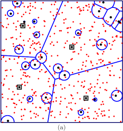
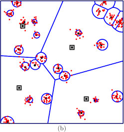
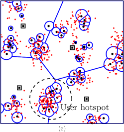
Figure 1: (a) Coverage-centric deployments where users are uniformly and independently distributed (our original $K$-tier HetNet model [12]), (b) user-centric deployment where users are clustered around SBSs (recent enhancement to the $K$-tier model [41]), and (c) user-centric deployment where users and SBSs are clustered around geographical centers of user hotspots (this paper). Black squares, black dots, and small red dots denote the locations of macro BSs, SBSs, and users, respectively.

II-A Spatial Setup and Key Assumptions

We model the locations of macro BSs as an independent homogeneous PPP $\{{\bf z}_{\rm m}\}\equiv\Phi_{\rm m}$ with density $\lambda_{\rm m}$. In order to capture the coupling between the locations of SBSs and users in hotspots, we model the locations of SBSs and users as two Poisson cluster processes with the same parent point process, where the later models the geographical centers of user hotspots. It should be noted that in reality user distribution is a superposition of homogeneous and non-homogeneous distributions. For instance, pedestrians and users in transit are more likely to be uniformly distributed in the network and hence homogeneous PPP is perhaps a better choice for the analysis of such users. On the other hand, users in hotspots exhibit clustering behavior for which Poisson cluster process is a more appropriate model than a homogeneous PPP [41]. The framework provided in this paper can be extended to the case of mixed user distribution consisting of both homogeneous and non-homogeneous user distributions without much effort. Besides, the analysis of homogeneous user distributions in such setups is well known [12, 8, 9, 10], which is the reason we chose to focus on the more challenging case of non-homogeneous user distributions in which the user and SBS locations are coupled.

Poisson cluster process can be formally defined as a union of offspring points which are independent of each other, and identically distributed around parent points [54, 55]. Modeling the locations of parent point process (i.e., cluster centers) as a homogeneous PPP $\{{\bf x}\}\equiv\Psi_{\rm p}$ with density $\lambda_{\rm p}$,

1. the set of users within a cluster centered at ${\bf x}\in\Psi_{\rm p}$ is denoted by $\{{\bf y}_{\rm u}\}\equiv{\cal N}^{\bf x}_{\rm u}$ (with ${\bf y}_{\rm u}\in\mathbb{R}^{2}$), where each set contains a sequence of i.i.d. elements conditional on $\mathbf{x}$ (denoting locations), and the PDF of each element is $f_{{\bf Y}_{\rm u}}({\bf y}_{\rm u})$, and

2. the set of SBSs within a cluster centered at ${\bf x}\in\Psi_{\rm p}$ is denoted by $\{{\bf y}_{\rm s}\}\equiv{\cal N}^{\bf x}_{\rm s}$ (with ${\bf y}_{\rm s}\in\mathbb{R}^{2}$), where each set contains a sequence of i.i.d. elements conditional on $\mathbf{x}$, and the PDF of each element is $f_{{\bf Y}_{\rm s}}({\bf y}_{\rm s})$.

The locations of SBSs ${\cal N}^{\bf x}_{\rm s}$ and users ${\cal N}^{\bf x}_{\rm u}$ conditioned on ${\bf x}\in\Psi_{\rm p}$ are independent. For this setup, after characterizing all theoretical results in terms of general distributions $f_{{\bf Y}_{\rm s}}({\bf y}_{\rm s})$ and $f_{{\bf Y}_{\rm u}}({\bf y}_{\rm u})$, we specialize the results to Thomas cluster process [56] in which the points are distributed around cluster centers according to an independent Gaussian distribution:

$$f_{{\bf Y}_{\ell}}({\bf y}_{\ell})=\frac{1}{2\pi\sigma_{\ell}^{2}}\exp\left(-\frac{\|{\bf y}_{\ell}\|^{2}}{2\sigma_{\ell}^{2}}\right),\>\text{where}\>{\ell}\in\{{\rm s},{\rm u}\}.$$ (1)

From the set of SBSs located in the cluster centered at ${\bf x}\in\Psi_{\rm p}$, we assume that the subset of ${\cal B}^{\bf x}_{\rm s}\subseteq{{\cal N}^{\bf x}_{\rm s}}$ reuse the same resource block. This subset will be henceforth referred to as a set of simultaneously active SBSs, where the number of simultaneously active SBSs $|{\cal B}^{\bf x}_{\rm s}|$ is assumed to have a Poisson distribution with mean $\bar{n}_{\rm as}$. Denote by ${{\bf x}_{0}}\in\Psi_{\rm p}$ the location of the center of representative cluster. In order to simplify the order statistics arguments that will be used in the selection of candidate serving BSs in the cluster located at ${\bf x}\in\Psi_{\rm p}$, we assume that the total number of SBSs (i.e., $|{{\cal N}^{{\bf x}_{0}}_{\rm s}}|$) in the representative cluster is fixed and equal to $n_{{\rm s}_{0}}$, where ${\cal B}^{{\bf x}_{0}}_{\rm s}\subseteq{\cal N}^{{\bf x}_{0}}_{\rm s}$ represents the set of simultaneously active SBSs in the representative cluster. Note that $|{\cal B}_{\rm s}^{{\bf x}_{0}}|$ is truncated Poisson random variable with maximum value being $n_{{\rm s}_{0}}$, and the serving SBS will be chosen from amongst SBS in ${\cal N}_{\rm s}^{{\bf x}_{0}}$. The pictorial representation of our setup along with the system models used in the prior work are presented in Fig. 1.

II-B Propagation Model

We assume that all links to the typical user suffer from a standard power-law path-loss with exponent $\alpha>2$, and Rayleigh fading. Thus the received power at the typical user (located at the origin) from the $j^{th}$ tier BS (where $j\in\{{\rm s},{\rm m}\}$) located at ${\bf z}_{j}$ is:

$$P_{\rm r}=P_{j}h_{j}\|{\bf z}_{j}\|^{-\alpha};\quad j\in\{{\rm s},{\rm m}\},$$ (2)

where $\|\cdot\|^{-\alpha}$ models power-law path-loss, $h_{j}$ is exponential random variable with unit mean independent of all other random variables, and $P_{j}$ is transmit power, which is assumed to be constant for the BSs in tier $j\in\{{\rm s},{\rm m}\}$. Note that index ‘${\rm m}$’ and ‘${\rm s}$’ refer to macro tier and small cell tier, respectively. Denote by $\{{\bf z}_{\rm s}={\bf x}_{0}+{{\bf y}_{\rm s}};{{\bf y}_{\rm s}}\in{\cal N}^{{\bf x}_{0}}_{\rm s}\}\equiv\Phi_{\rm s}$ the locations of open-access SBSs. The candidate serving BS location from $\Phi_{j}$ is:

$${{\bf z}^{*}_{j}}=\operatorname{arg~{}max}_{{{\bf z}_{j}}\in\Phi_{j}}P_{j}\|{\bf z}_{j}\|^{-\alpha},$$ (3)

where ${{\bf z}^{*}_{j}}$ is the location of the nearest open-access BS of the $j^{th}$ tier (i.e., $\Phi_{j}$) to the typical user. In order to select the serving BS from amongst the set of candidate serving BSs, we consider two association policies. In Policy 1, the goal is to maximize coverage probability and hence the reference signal received power (RSRP), which is the average received power of all open-access BSs measured by a typical user, are compered and the user is served by the BSs which provides maximum average received power. In Policy 2, the goal is to balance the load across the network, and hence user is served by small cell tier if maximum RSRP from open access SBSs is greater than specific power threshold; and macro tier otherwise. More details on these two association policies will be provided in the next Section.

II-B1 $\mathtt{SIR}$ at a typical user served by macrocell

Assuming that the typical user is served by the macro BS located at ${\bf z}^{*}$, the total interference seen at the typical user originates from three sources: (i) interference caused by macro BSs (except the serving BS) defined as: ${\cal I}_{\rm mm}=\sum_{{\bf z}_{\rm m}\in\Phi_{\rm m}\setminus{{\bf z}^{*}}}P_{\rm m}h_{\rm m}\|{\bf z}_{\rm m}\|^{-\alpha}$, (ii) intra-cluster interference caused by simultaneously active open-access SBSs inside the representative cluster (i.e., typical user’s cluster), which is defined as: ${\cal I}_{\rm sm}^{\rm intra}=\sum_{{\bf y}_{\rm s}\in{\cal B}_{\rm s}^{{\bf x}_{0}}}P_{\rm s}h_{\rm s}\|{\bf x}_{0}+{\bf y}_{\rm s}\|^{-\alpha}$, and (iii) inter-cluster interference caused by simultaneously active closed-access SBSs outside the representative cluster defined as: ${\cal I}_{\rm sm}^{\rm inter}=\sum_{{\bf x}\in\Psi_{\rm p}\setminus{\bf x}_{0}}\sum_{{\bf y}_{\rm s}\in{\cal B}_{\rm s}^{{\bf x}}}\\ P_{\rm s}h_{\rm s}\|{\bf x}+{\bf y}_{\rm s}\|^{-\alpha}$. The $\mathtt{SIR}$ at the typical user conditioned on the serving BS being macrocell is:

$${\tt SIR}_{\rm m}=\frac{P_{\rm m}h_{\rm m}\|{\bf z}^{*}\|^{-\alpha}}{{\cal I}_{\rm mm}+{\cal I}_{\rm sm}^{\rm intra}+{\cal I}_{\rm sm}^{\rm inter}}.$$ (4)

II-B2 $\mathtt{SIR}$ at a typical user served by small cell

Assuming that a typical user is served by the SBS located at ${\bf z}^{*}={\bf x}_{0}+{\bf y}_{0}$, the contribution of the total interference seen at the typical user can be partitioned into three sources: (i) interference from macro BSs defined as: ${\cal I}_{\rm ms}=\sum_{{\bf z}_{\rm m}\in\Phi_{\rm m}}P_{\rm m}h_{\rm m}\|{\bf z}_{\rm m}\|^{-\alpha}$, (ii) interference from simultaneously active open-access SBSs (except the serving BS) inside the representative cluster defined as: ${{\cal I}_{\rm ss}^{\rm intra}=\sum_{{\bf y}_{\rm s}\in{\cal B}_{\rm s}^{{\bf x}_{0}}\setminus{{\bf y}_{0}}}P_{\rm s}h_{\rm s}\|{\bf x}_{0}+{\bf y}_{\rm s}\|^{-\alpha}}$, and (iii) interference from simultaneously active closed-access SBSs outside the representative cluster defined as: ${\cal I}_{\rm ss}^{\rm inter}=\sum_{{\bf x}\in{\Psi_{\rm p}}\setminus{\bf x}_{0}}\sum_{{\bf y}_{\rm s}\in{\cal B}_{\rm s}^{{\bf x}}}P_{\rm s}h_{\rm s}\|{\bf x}+{\bf y}_{\rm s}\|^{-\alpha}$. Therefore, the $\mathtt{SIR}$ at the typical user served by the small cell is:

$${\tt SIR}_{\rm s}=\frac{P_{\rm s}h_{\rm s}\|{\bf z}^{*}\|^{-\alpha}}{{\cal I}_{\rm ms}+{\cal I}_{\rm ss}^{\rm intra}+{\cal I}_{\rm ss}^{\rm inter}}.$$ (5)

TABLE I: Summary of notation

Notation	Description
$\Phi_{\rm m};\ \lambda_{\rm m}$	Independent PPP modeling the locations of macro BSs; density of $\Phi_{\rm m}$
$\Psi_{\rm p};\ \lambda_{\rm p}$	Independent PPP modeling the locations of parent points (cluster centers); density of $\Psi_{\rm p}$
${\cal N}^{{\bf x}}_{\rm s};\ {\cal N}^{{\bf x}}_{\rm u}$	Set of SBSs in a cluster centered at ${\bf x}\in\Psi_{\rm p}$; Set of users in a cluster centered at ${\bf x}\in\Psi_{\rm p}$
${\cal B}^{{\bf x}}_{\rm s}\subseteq{\cal N}^{{\bf x}}_{\rm s};\bar{n}_{\rm as}$	Set of simultaneously active SBSs in a cluster centered at ${\bf x}\in\Psi_{\rm p}$ with mean $\bar{n}_{\rm as}$
$\sigma_{\rm s}^{2}$ ($\sigma_{\rm u}^{2}$)	Scattering variance of the SBS (user) locations around each cluster center
$P_{j}$; $h_{j}$; $\alpha$; $\beta$	Transmit power; channel power gain under Rayleigh fading; path loss exponent; target $\mathtt{SIR}$
${\cal A}_{j}^{\rm P1}$ $({\cal A}_{j}^{\rm P2})$	Association probability under association Policy 1 (Policy 2), where $j\in\{{\rm s},{\rm m}\}$
${\tt P}^{\rm P1}_{{\rm c}_{j}}$ $({\tt P}^{\rm P2}_{{\rm c}_{j}})$	Coverage probability of a typical user served by tier $j\in\{{\rm s},{\rm m}\}$ under association Policy 1 (Policy 2)
${\tt P}^{\rm P1}_{{\rm c}_{\rm T}}$ $({\tt P}^{\rm P2}_{{\rm c}_{\rm T}})$	Total coverage probability under association Policy 1 (Policy 2)
${\cal T}^{\rm P1}$ $({\cal T}^{\rm P2})$	Throughput under association Policy 1 (Policy 2)

III Serving and Interfering Distances

This is the first main technical section of the paper, where we derive the association probability of a typical user to macro BSs and SBSs. We then characterize the distributions of distances from serving and interfering macro BSs and SBSs to a typical user. These distance distributions will be used to characterize the coverage probability of a typical user, and throughput of the whole network in the next section. We now begin by providing relevant distance distributions.

III-A Relevant distance distributions

Let us denote the distances from a typical user to its nearest open-access SBS and macro BS by $R_{\rm s}$ and ${R_{\rm m}}$, respectively. In order to calculate the association probability and the serving distance distribution, it is important to first characterize the density functions of $R_{\rm m}$ and $R_{\rm s}$. The PDF and CDF of the distance from a typical user to its nearest macro BS, i.e., $R_{\rm m}$, can be easily obtained by using null probability of a homogeneous PPP as [57]:

$$\text{PDF:}\quad f_{R_{\rm m}}(r_{\rm m})=2\pi\lambda_{\rm m}r_{\rm m}\exp(-\pi\lambda_{\rm m}r_{\rm m}^{2})\quad \text{ CDF:}\quad F_{R_{\rm m}}(r_{\rm m})=1-\exp(-\pi\lambda_{\rm m}r_{\rm m}^{2}).$$ (6)

However, characterizing the density function of distance from a typical user to its nearest open-access SBS, i.e., the nearest SBS to the typical user from representative cluster, is more challenging. To derive the density function of $R_{\rm s}$, it is useful to define the sequence of distances from the typical user to the SBSs located within the representative cluster as ${\cal D}^{{\bf x}_{0}}_{\rm s}=\{{u:u=\|{\bf x}_{0}+{\bf y}_{\rm s}\|},\forall{\bf y}_{\rm s}\in{\cal N}^{{\bf x}_{0}}_{\rm s}\}$. Note that the elements in ${\cal D}^{{\bf x}_{0}}_{\rm s}$ are correlated due to the common factor ${\bf x}_{0}$. But this correlation can be handled by conditioning on the location of representative cluster center ${\bf x}_{0}$ because the SBS locations are i.i.d. around the cluster center by assumption. The conditional PDF of any (arbitrary) element in the set ${\cal D}^{{\bf x}_{0}}_{\rm s}$ is characterized next.

Lemma 1.

The distances in the set ${\cal D}^{{\bf x}_{0}}_{\rm s}$ conditioned on the distance of the typical user to the cluster center, i.e., $V_{0}=\|{\bf x}_{0}\|$, are i.i.d., where the CDF of each element for a given $V_{0}=\nu_{0}$ is:

$$F_{U}(u|\nu_{0})=\int_{z_{1}=-u}^{z_{1}=u}\int_{z_{2}=-\sqrt{u^{2}-z_{1}^{2}}}^{z_{2}=\sqrt{u^{2}-z_{1}^{2}}}f_{{\bf Y}_{\rm s}}(z_{1}-\nu_{0},z_{2}){\rm d}{z_{2}}{\rm d}z_{1},$$ (7)

and the conditional PDF of $U$ is:

$$f_{U}(u|\nu_{0})=\int_{-u}^{u}\frac{u}{\sqrt{u^{2}-z_{1}^{2}}}\Big{[}f_{{\bf Y}_{\rm s}}\Big{(}z_{1}-\nu_{0},\sqrt{u^{2}-z_{1}^{2}}\Big{)}+f_{{\bf Y}_{\rm s}}\Big{(}z_{1}-\nu_{0},-\sqrt{u^{2}-z_{1}^{2}}\Big{)}\Big{]}{\rm d}z_{1},$$ (8)

where the PDF of $V_{0}$ is given by

$$f_{V_{0}}(\nu_{0})=\int_{-\nu_{0}}^{\nu_{0}}\frac{\nu_{0}}{\sqrt{\nu_{0}^{2}-x_{1}^{2}}}\Big{[}f_{{\bf Y}_{\rm u}}\Big{(}x_{1},\sqrt{v_{0}^{2}-x_{1}^{2}}\Big{)}+f_{{\bf Y}_{\rm u}}\Big{(}x_{1},-\sqrt{v_{0}^{2}-x_{1}^{2}}\Big{)}\Big{]}{\rm d}x_{1}.$$ (9)

Proof:

See Appendix -A. ∎

The density functions of distances presented in Lemma 1 are specialized to the case of Thomas cluster process in the next Corollary.

Corollary 1.

For the special case of Thomas cluster process, the distances in the set ${\cal D}^{{\bf x}_{0}}_{\rm s}$ are conditionally i.i.d., with CDF

$$F_{U}(u|\nu_{0})=1-Q_{1}\Big{(}\frac{\nu_{0}}{\sigma_{\rm s}},\frac{u}{\sigma_{\rm s}}\Big{)},\quad u>0,$$ (10)

where $Q_{1}(a,b)$ is the Marcum Q-function defined as $Q_{1}(a,b)=\int_{b}^{\infty}te^{-\frac{t^{2}+a^{2}}{2}}I_{0}(at){\rm d}t$, and the PDF of each element is:

$$f_{U}(u|\nu_{0})=\frac{u}{\sigma_{\rm s}^{2}}\exp\left(-\frac{u^{2}+\nu_{0}^{2}}{2\sigma_{\rm s}^{2}}\right)I_{0}\left(\frac{u\nu_{0}}{\sigma_{\rm s}^{2}}\right),\quad u>0,$$ (11)

where $I_{0}(\cdot)$ is the modified Bessel function of the first kind with order zero. The PDF of $V_{0}$ is:

$$f_{V_{0}}(\nu_{0})=\frac{\nu_{0}}{\sigma_{\rm u}^{2}}\exp\left(-\frac{\nu_{0}^{2}}{2\sigma_{\rm u}^{2}}\right),\quad\nu_{0}>0.$$ (12)

Proof:

For the special case of Thomas cluster process, the PDF of ${\bf Y}_{\rm s}$ with realization ${\bf y}_{\rm s}=(y_{\rm s_{1}},y_{\rm s_{2}})$ can be expressed as:

$$f_{{\bf Y}_{s}}(y_{\rm s_{1}},y_{\rm s_{2}})=\frac{1}{2\pi\sigma_{\rm s}^{2}}\exp\left(-\frac{{y_{\rm s_{1}}^{2}+y_{\rm s_{2}}^{2}}}{2\sigma_{\rm s}^{2}}\right).$$

Substituting $f_{{\bf Y}_{s}}(\cdot)$ into (8) and letting $z_{1}=u\cos{\theta}$, we get Rician distribution as:

$$f_{U}(u|\nu_{0})=\frac{u}{\sigma_{\rm s}^{2}}\exp(-\frac{u^{2}+\nu_{0}^{2}}{2\sigma_{\rm s}^{2}})\underbrace{\int_{-\pi/2}^{\pi_{2}}\frac{1}{2\pi}\exp(\frac{u\nu_{0}\cos\theta}{\sigma_{\rm s}^{2}})}_{I_{0}(\frac{u\nu_{0}}{\sigma_{\rm s}^{2}})}{\rm d}\theta,$$

where $F_{U}(u|\nu_{0})=1-\int_{u}^{\infty}f_{U}(u|\nu_{0}){\rm d}u$. Similarly, the PDF of $V_{0}$ can be obtained by substituting (1) in (9), where $V_{0}$ has a Rayleigh distribution with scale parameter $\sigma_{\rm u}$. ∎

The conditional i.i.d. property of distances in the set ${\cal D}^{{\bf x}_{0}}_{\rm s}$ enables us to characterize the distance from the typical user to its nearest open-access SBS located within the representative cluster. This result is presented in the next Lemma.

Lemma 2.

Conditioned on the distance of the typical user to its cluster center, i.e. $V_{0}$, the CDF of distance from the typical user to its nearest open-access SBS, i.e., $R_{\rm s}$, for a given $V_{0}=\nu_{0}$ is:

$$F_{R_{\rm s}}(r_{\rm s}|\nu_{0})=1-(1-F_{U}(r_{\rm s}|\nu_{0}))^{n_{{\rm s}_{0}}},$$ (13)

and the conditional PDF of $R_{\rm s}$ for a given $\nu_{0}$ is:

$$f_{R_{\rm s}}(r_{\rm s}|\nu_{0})=n_{{\rm s}_{0}}(1-F_{U}(r_{\rm s}|\nu_{0}))^{n_{{\rm s}_{0}}-1}f_{U}(r_{\rm s}|\nu_{0}),$$ (14)

where $F_{U}(\cdot|\nu_{0})$ and $f_{U}(\cdot|\nu_{0})$ are given by (7) and (8), respectively.

Proof:

Conditioned on the distance of the typical user to its cluster center, the elements in ${\cal D}^{{\bf x}_{0}}_{\rm s}$ are i.i.d. with PDF $f_{U}(\cdot|\nu_{0})$. Thus the result simply follows from the PDF of the minimum element of the i.i.d. sequence of random variables [58, eqn. (3)]. ∎

These distance distributions are the keys to the derivation of the metrics of interest.

III-B Association policies

As discussed above, the candidate serving BS in each open-access tier (i.e., all macro BSs and SBSs located within the representative cluster) is the one nearest to the user. Recall that the distances from a typical user to its nearest open-access small cell and macro BSs were denoted by $R_{\rm s}$ and ${R_{\rm m}}$, respectively. In order to select the serving BS from amongst the candidate serving BSs, we consider the following two association policies.

III-B1 Association Policy 1

The serving BS is chosen from amongst the candidate serving BSs according to maximum received-power averaged over small-scale fading. As noted earlier, this association policy maximizes coverage probability of a typical user. The association event to macro BSs and SBSs can be formally defined as follows.

• A typical user is associated to a macrocell if $\operatorname{arg~{}max}_{j\in\{{\rm s},{\rm m}\}}P_{j}R_{j}^{-\alpha}={\rm m}$. The association event to macrocell is denoted by $S_{\rm m}^{\rm P1}$, where ${\bf 1}_{S_{\rm m}^{\rm P1}}={\bf 1}(\operatorname{arg~{}max}_{j\in\{{\rm s},{\rm m}\}}P_{j}R_{j}^{-\alpha}={\rm m}).$

• A typical user is associated to a small cell if $\operatorname{arg~{}max}_{j\in\{{\rm s},{\rm m}\}}P_{j}R_{j}^{-\alpha}={\rm s}$. The association event to the small cell is denoted by $S_{\rm s}^{\rm P1}$, where ${\bf 1}_{S_{\rm s}^{\rm P1}}={\bf 1}(\operatorname{arg~{}max}_{j\in\{{\rm s},{\rm m}\}}P_{j}R_{j}^{-\alpha}={\rm s}).$

Now, the density functions of distances $f_{R_{\rm s}}(\cdot|\nu_{0})$ and $f_{R_{\rm m}}(\cdot)$ obtained in the previous subsection are used to characterize the association probabilities to macro and small cells in the next Lemma.

Lemma 3 (Association probability for Policy 1).

The association probability of a typical user located at distance $\nu_{0}$ from its cluster center to the macrocell tier is:

$${\cal A}_{\rm m}^{\rm P1}(\nu_{0})=\int_{0}^{\infty}\big{[}1-F_{R_{\rm s}}\big{(}\xi_{\rm sm}r_{\rm m}|\nu_{0}\big{)}\big{]}f_{R_{\rm m}}(r_{\rm m}){\rm d}r_{\rm m},$$ (15)

with $\xi_{\rm sm}=\big{(}\frac{P_{\rm s}}{P_{\rm m}}\big{)}^{1/\alpha}$, and the association probability to the small cell tier is:

$${\cal A}_{\rm s}^{\rm P1}(\nu_{0})=1-{\cal A}_{\rm m}^{\rm P1}(\nu_{0}),$$ (16)

where $f_{R_{\rm m}}(\cdot)$ and $F_{R_{\rm s}}(\cdot|\nu_{0})$ are given by (6) and (13), respectively.

Proof:

See Appendix -B. ∎

The serving distance is simply the distance from the typical user to its nearest BS from associated tier. Denote by $X^{\rm P1}_{j}$ the serving distance to tier $j\in\{{\rm m},{\rm s}\}$. The density function of $X^{\rm P1}_{j}$ is characterized in the next Lemma.

Lemma 4 (Serving distance distribution under association Policy 1).

For a typical user located at distance $\nu_{0}$ from its cluster center, the PDF of serving distance $X_{\rm m}^{\rm P1}$ conditioned on the association to macrocell, i.e., event $S_{\rm m}^{\rm P1}$, is:

$$f_{X_{\rm m}^{\rm P1}}(x_{\rm m}|\nu_{0})=\frac{1}{{\cal A}^{\rm P1}_{\rm m}(\nu_{0})}(1-F_{R_{\rm s}}(\xi_{\rm sm}x_{\rm m}|\nu_{0}))f_{R_{\rm m}}(x_{\rm m}),\text{ and}$$ (17)

the PDF of $X_{\rm s}^{\rm P1}$ conditioned on the association to small cell, i.e., event $S_{\rm s}^{\rm P1}$, is:

$$f_{X_{\rm s}^{\rm P1}}(x_{\rm s}|\nu_{0})=\frac{1}{{\cal A}^{\rm P1}_{\rm s}(\nu_{0})}(1-F_{R_{\rm m}}(\xi_{\rm ms}x_{\rm s}))f_{R_{\rm s}}(x_{\rm s}|\nu_{0}),$$ (18)

where $\xi_{\rm sm}=\big{(}\frac{P_{\rm s}}{P_{\rm m}}\big{)}^{1/\alpha}$ and $\xi_{\rm ms}=\big{(}\frac{P_{\rm m}}{P_{\rm s}}\big{)}^{1/\alpha}$. The density functions of distances $f_{R_{\rm m}}(\cdot)$, $f_{R_{\rm s}}(\cdot|\nu_{0})$, and $F_{R_{\rm s}}(\cdot|\nu_{0})$ are given by (6), (14), and (13), respectively.

Proof:

See Appendix -C. ∎

From association Policy 1, it can be deduced that there are no open-access BSs within distance $\xi_{\rm ms}x_{\rm s}$ ($\xi_{\rm sm}x_{\rm m}$) of the typical user when this user is served by small cell (macrocell) BS. This can be interpreted as an exclusion zone with radius $\xi_{\rm ms}x_{\rm s}$ or $\xi_{\rm sm}x_{\rm m}$ depending upon the choice of serving BS, which is centered at the location of the typical user. The effect of exclusion zone on the interference caused by macro BSs (distributed according to a homogeneous PPP $\Phi_{\rm m}$) can be easily handled using the fact that the distribution of the PPP conditioned on the location of a point of PPP (here serving BS) is the same as that of the original PPP [56]. However, characterizing the effect of exclusion zone on the distribution of distances from clustered open-access interfering SBSs to the typical user is more challenging. We define the set ${\cal F}^{\rm P1}_{\rm s}({\cal F}^{\rm P1}_{\rm m})$ to represent the sequence of distances from open access interfering SBSs (which by assumption belong to the representative cluster centered at ${\bf x}_{0}$) to the typical user conditioned on the serving BS belonging to small cell (macrocell), such that the elements of $W^{\rm P1}_{\rm s}\in{\cal F}^{\rm P1}_{\rm s}$ and $W^{\rm P1}_{\rm m}\in{\cal F}^{\rm P1}_{\rm m}$ are greater than $\xi_{\rm ms}x_{\rm s}$ and $\xi_{\rm sm}x_{\rm m}$, respectively. In the next Lemma, we deal with the conditional i.i.d. property of the elements of ${\cal F}^{\rm P1}_{\rm s}$ and ${\cal F}^{\rm P1}_{\rm m}$, and their distributions.

Lemma 5 (Policy 1: distribution of distances from open-access interfering SBSs).

Under association Policy 1, the elements of ${\cal F}^{\rm P1}_{\rm m}\ ({\cal F}^{\rm P1}_{\rm s})$ conditioned on $V_{0}$ and $X^{\rm P1}_{\rm m}(X^{\rm P1}_{\rm s})$ are i.i.d., where the PDF of each element $W^{\rm P1}_{\rm m}\in{\cal F}^{\rm P1}_{\rm m}$ for a given $V_{0}=\nu_{0}$ and $X^{\rm P1}_{\rm m}=x_{\rm m}$ is:

$$f_{W^{\rm P1}_{\rm m}}(w_{\rm m}|\nu_{0},x_{\rm m})=\frac{f_{U}(w_{\rm m}|\nu_{0})}{1-F_{U}(\xi_{\rm sm}x_{\rm m}|\nu_{0})},$$ (19)

and the conditional PDF of each element $W^{\rm P1}_{\rm s}\in{\cal F}^{\rm P1}_{\rm s}$ is:

$$f_{W^{\rm P1}_{\rm s}}(w_{\rm s}|\nu_{0},x_{\rm s})=\frac{f_{U}(w_{\rm s}|\nu_{0})}{1-F_{U}(x_{\rm s}|\nu_{0})},$$ (20)

where $F_{U}(\cdot|\nu_{0})$ and $f_{U}(\cdot|\nu_{0})$ are given by (7) and (8), respectively.

Proof:

See Appendix -D. ∎

III-B2 Association Policy 2

In addition to maximum RSRP-based association policy discussed above, it is often times desirable to define simple canonical association policies to balance load across the network, which we do next. For this purpose, the association event to the SBS and macro BS is defined as follows.

• A typical user is associated to the small cell if $P_{\rm s}{R_{\rm s}}^{-\alpha}\geq P_{0}$. The association event to the small cell is denoted by $S_{\rm s}^{\rm P2}$, where ${\bf 1}_{S_{\rm s}^{\rm P2}}={\bf 1}({R_{\rm s}}\leq D)$ and $D\equiv\Big{(}\frac{P_{\rm 0}}{P_{\rm s}}\Big{)}^{-1/\alpha}$.

• A typical user is associated to the macrocell if $P_{\rm s}{R_{\rm s}}^{-\alpha}\leq P_{0}$. The association event to the macrocell is denoted by $S_{\rm m}^{\rm P2}$, where ${\bf 1}_{S_{\rm m}^{\rm P2}}={\bf 1}({R_{\rm s}}\geq D).$

Here $P_{0}$ denotes the SBS power threshold. In contrast to the association Policy 1, which is a function of the distances from both the nearest macro and small cell BSs to a typical user, the association Policy 2 is only a function of the distance of a typical user to its nearest open-access SBS, which lends relatively more tractability to the analysis. This simple policy allows us to balance load across macro and small cells by tuning the value of $P_{0}$. The exact impact of $P_{0}$ on the coverage probability will be studied in the later sections. According to the definition of $S_{\rm s}^{\rm P2}$, the conditional association probability to the small cell tier for a given $V_{0}=\nu_{0}$ is:

$${\cal A}_{\rm s}^{\rm P2}(\nu_{0})=\mathbb{E}_{R_{\rm s}}[{\bf 1}(R_{\rm s}<D)|\nu_{0}]=\mathbb{P}(R_{\rm s}<D|\nu_{0})=F_{R_{\rm s}}(D|\nu_{0}),$$ (21)

and the association probability to the macrocell tier is:

$${\cal A}^{\rm P2}_{\rm m}(\nu_{0})=1-{\cal A}_{\rm s}^{\rm P2}(\nu_{0}).$$ (22)

Using the macro and small cell association probabilities, the density function of serving distance is derived in the next Lemma.

Lemma 6 (Serving distance PDF for association Policy 2).

The PDF of serving distance $X^{\rm P2}_{\rm s}$ when the typical user located at distance $\nu_{0}$ from its own cluster center is served by a small cell is:

$$f_{X^{\rm P2}_{\rm s}}(x_{\rm s}|\nu_{0})=\frac{f_{R_{\rm s}}(x_{\rm s}|\nu_{0})}{{\cal A}^{\rm P2}_{\rm s}(\nu_{0})},\quad 0\leq x_{\rm s}\leq D,$$ (23)

and the PDF of serving serving distance $X^{\rm P2}_{\rm s}$ when the typical user is served by a macrocell is:

$$f_{X^{\rm P2}_{\rm m}}(x_{\rm m})={f_{R_{\rm m}}(x_{\rm m})},\quad x_{\rm m}\geq 0,$$ (24)

where ${f_{R_{\rm m}}(\cdot)}$, $f_{R_{\rm s}}(\cdot|\nu_{0})$ and ${{\cal A}^{\rm P2}_{\rm s}(\nu_{0})}$ are given by (6), (14), and (21), respectively.

Proof:

For the typical user located at distance $\nu_{0}$ from its own cluster center, $f_{X^{\rm P2}_{\rm s}}(x_{\rm s}|\nu_{0})$ is the PDF of distance from the typical user to its nearest open-access SBS conditioned on the association to small cell tier $S_{\rm s}^{\rm P2}$, which is equal to $f_{R_{\rm s}}(x_{\rm s}|S^{\rm P2}_{\rm s},\nu_{0})$. However, the association to the macrocell is independent of the distance from the typical user to its nearest macro BS. Thus the PDF of serving distance when the typical user is served by macrocell is simply the PDF of distance to its nearest macro BS. ∎

As has already been discussed earlier, the locations of open-access interfering BSs depend upon the association event. From association Policy 2, it can be deduced that if a typical user is served by small cell (macrocell), the closest open-access interfering SBS must be at distance greater than $x_{\rm s}$ ($D\equiv\Big{(}\frac{P_{\rm 0}}{P_{\rm s}}\Big{)}^{-1/\alpha}$) from the typical user. Denote by ${\cal F}^{\rm P2}_{\rm s}$ (${\cal F}^{\rm P2}_{\rm m}$) the sequence of distances from intra-cluster interfering SBSs to the typical user served by small cell (macrocell). The distributions of the elements of ${\cal F}^{\rm P2}_{\rm s}$ and ${\cal F}^{\rm P2}_{\rm m}$ are given in the next Lemma.

Lemma 7 (Association Policy 2: distribution of distances from open-access interfering SBSs).

The elements in the sequence of distances from open-access interfering SBSs to the typical user served by macrocell, i.e., ${\cal F}^{\rm P2}_{\rm m}$, conditioned on $V_{0}$ are i.i.d., where the PDF of each element $W^{\rm P2}_{\rm m}\in{\cal F}^{\rm P2}_{\rm m}$ is:

$$f_{W^{\rm P2}_{\rm m}}(w_{\rm m}|\nu_{0})=\frac{f_{U}(w_{\rm m}|\nu_{0})}{1-F_{U}(D|\nu_{0})},$$ (25)

and the elements in the sequence of distances from open-access interfering SBSs to the typical user served by small cell, i.e., ${\cal F}^{\rm P2}_{\rm s}$, are conditionally i.i.d., where the PDF of each element $W^{\rm P2}_{\rm s}\in{\cal F}^{\rm P2}_{\rm m}$ for given $V_{0}=\nu_{0}$ and $X^{\rm P2}_{\rm s}=x_{\rm s}$ is:

$$f_{W^{\rm P2}_{\rm s}}(w_{\rm s}|\nu_{0},x_{\rm s})=\frac{f_{U}(w_{\rm s}|\nu_{0})}{1-F_{U}(x_{\rm s}|\nu_{0})},$$ (26)

where $F_{U}(\cdot|\nu_{0})$ and $f_{U}(\cdot|\nu_{0})$ are given by (7) and (8), respectively.

Proof:

The proof follows on the same lines as that of Lemma 5, and is hence skipped. ∎

The locations of closed-access interfering SBSs are independent of association policy. Thus the distribution of distances from the typical user to the closed-access SBSs (also called inter-cluster interfering SBSs) is the same for association policies 1 and 2. This distribution is presented next.

Lemma 8 (Distribution of distances from closed-access interfering SBSs).

Denote by ${\cal D}^{\bf x}_{\rm s}=\{t_{\rm s}:t_{\rm s}=\|{\bf x}+{\bf y}_{\rm s}\|,\forall\ {\bf y}_{\rm s}\in{\cal N}^{\bf x}_{\rm s}\}$ the sequence of distances from the typical user to inter-cluster interfering SBSs within the cluster centered at ${\bf x}\in\Psi_{\rm p}$. For a given $v=\|{\bf x}\|$, the elements of ${\cal D}^{\bf x}_{\rm s}$ are i.i.d., with PDF

$$f_{T_{\rm s}}(t_{\rm s}|\nu)=\int_{-t_{\rm s}}^{t_{\rm s}}\frac{t_{\rm s}}{\sqrt{t_{\rm s}^{2}-z^{2}}}\Big{[}f_{{\bf Y}_{\rm s}}\big{(}z-\nu,\sqrt{t_{\rm s}^{2}-z^{2}}\big{)}+f_{{\bf Y}_{\rm s}}\big{(}z-\nu,-\sqrt{t_{\rm s}^{2}-z^{2}}\big{)}\Big{]}{\rm d}z,\ t_{\rm s}>0.$$ (27)

Proof:

The elements of the sequence ${\cal N}^{\bf x}_{\rm s}$, i.e., relative locations of the SBSs to the cluster centered at ${\bf x}\in{\Psi}_{\rm p}$, are i.i.d. by assumption. Hence, for a given $\nu=\|{\bf x}\|$, the elements of the sequence ${\cal D}^{\bf x}_{\rm s}$ are i.i.d. The derivation of $f_{T_{\rm s}}(\cdot|\nu)$ follows on the same lines as that of $f_{U}(\cdot|\nu_{0})$ given by (8), and hence is skipped. ∎

Remark 1 (Thomas cluster process).

For the special case of Thomas cluster process, the elements in the sequence of distances from closed-access interfering SBSs to the typical user are i.i.d., where the PDF of each element is:

$$f_{T_{\rm s}}(t_{\rm s}|\nu)=\frac{t_{\rm s}}{\sigma_{\rm s}^{2}}\exp\left(-\frac{t_{\rm s}^{2}+\nu^{2}}{2\sigma_{\rm s}^{2}}\right)I_{0}\left(\frac{t_{\rm s}\nu}{\sigma_{\rm s}^{2}}\right),\quad t_{\rm s}>0,$$ (28)

which is Rician. The proof is exactly the same as that of Corollary 1. It should be noted that all the results can be specialized to Thomas cluster process by substituting $F_{U}(\cdot|\nu_{0})$, $f_{U}(\cdot|\nu_{0})$, $f_{V_{0}}(\cdot)$, and $f_{T_{\rm s}}(\cdot|\nu)$ with the expressions given by (10), (11), (12), and (28), respectively.

IV Coverage Probability and Throughput Analysis

This is the second main technical section of this paper, where we use the distance distributions and association probabilities derived in the previous section to characterize network performance in terms of coverage probability of a typical user and throughput of the whole network.

IV-A Coverage probability

The coverage probability can be formally defined as the probability that $\mathtt{SIR}$ experienced by a typical user is greater than the desired threshold for successful demodulation and decoding. Mathematically, it is $\mathtt{P_{c}}=\mathbb{E}[{\bf 1}(\mathtt{SIR}>\beta)]=\mathbb{P}(\mathtt{SIR}>\beta)$, where $\beta$ is the target $\mathtt{SIR}$ threshold. We specialize this definition to the two association policies in this subsection. We begin our discussion with association Policy 1.

IV-A1 Association Policy 1

As evident in the sequel, the Laplace transform of (the PDF of) interference is the key intermediate result for the coverage probability analysis. Thus we first focus on the derivation of the Laplace transform of interference distribution. As has already been described earlier, the contribution of the total interference seen at a typical user can be partitioned into three sources: i) interference caused by open-access SBSs, ii) interference caused by closed-access SBSs, and iii) interference caused by macro BSs. We now use the distance distributions presented in Lemma 5 to characterize the Laplace transform of interference originating from the open-access SBSs (intra-cluster interferers) in the next Lemma.

Lemma 9.

Under association Policy 1, the conditional Laplace transform of interference distribution caused by open-access SBSs at a typical user served by macrocell, ${{\cal I}^{\rm intra}_{\rm sm}}$, for a given $X^{\rm P1}_{\rm m}=x_{\rm m}$ and $V_{0}=\nu_{0}$ is:

$${\cal L}^{\rm P1}_{{\cal I}^{\rm intra}_{\rm sm}}(s|\nu_{0},x_{\rm m})=\sum_{\ell=0}^{n_{\rm s_{0}}}\left(\int_{\xi_{\rm sm}x_{\rm m}}^{\infty}\frac{1}{1+sP_{\rm s}w_{\rm m}^{-\alpha}}f_{W^{\rm P1}_{\rm m}}(w_{\rm m}|\nu_{0},x_{\rm m}){\rm d}w_{\rm m}\right)^{\ell}\frac{\bar{n}_{\rm as}^{\ell}e^{-\bar{n}_{\rm as}}}{\ell!\sum_{k=0}^{n_{\rm s_{0}}}\frac{{\bar{n}_{\rm as}}^{k}e^{-\bar{n}_{\rm as}}}{k!}},$$ (29)

and the Laplace transform of interference distribution caused by open-access SBSs at a typical user served by small cell, ${{\cal I}^{\rm intra}_{\rm ss}}$, is:

$${\cal L}^{\rm P1}_{{\cal I}^{\rm intra}_{\rm ss}}(s|\nu_{0},x_{\rm s})=\sum_{\ell=1}^{n_{\rm s_{0}}}\left(\int_{x_{\rm s}}^{\infty}\frac{1}{1+sP_{\rm s}w_{\rm s}^{-\alpha}}f_{W^{\rm P1}_{\rm s}}(w_{\rm s}|\nu_{0},x_{\rm s}){\rm d}w_{\rm s}\right)^{\ell-1}\frac{{\bar{n}_{\rm as}}^{\ell-1}e^{-\bar{n}_{\rm as}}}{(\ell-1)!\sum_{k=1}^{n_{\rm s_{0}}}\frac{{\bar{n}_{\rm as}}^{k-1}e^{-\bar{n}_{\rm as}}}{(k-1)!}},$$ (30)

where $f_{W^{\rm P1}_{\rm m}}(\cdot|\nu_{0},x_{\rm m})$ and $f_{W^{\rm P1}_{\rm s}}(\cdot|\nu_{0},x_{\rm s})$ are given by Lemma 5.

Proof:

See Appendix -E. ∎

Recall that the total number of SBSs in the representative cluster was assumed to be known a priori and equal to $n_{\rm s_{0}}$. This assumption was made to simplify order statistics argument used in the derivation of the PDF of serving distance, but it constrains the maximum number of interfering SBSs in the representative cluster, which complicates the numerical evaluation of the exact coverage probability (will be presented in Theorem 1) due to the summation involved in the expressions given by Lemma 9. However, these expressions can be simplified under the assumption of $\bar{n}_{\rm as}\ll n_{{\rm s}_{0}}$, and the simplified expressions are presented in the next Corollary.

Corollary 2.

For $\bar{n}_{\rm as}\ll n_{{\rm s}_{0}}$, the Laplace transform of interference given by (29) reduces to

$${\cal L}^{\rm P1}_{{\cal I}^{\rm intra}_{\rm sm}}(s|\nu_{0},x_{\rm m})=\exp\Big{(}\bar{n}_{\rm as}\int_{\xi_{\rm sm}x_{\rm m}}^{\infty}\frac{1}{1+\frac{w_{\rm m}^{\alpha}}{sP_{\rm s}}}f_{W^{\rm P1}_{\rm m}}(w_{\rm m}|\nu_{0},x_{\rm m}){\rm d}w_{\rm m}\Big{)},$$ (31)

and the Laplace transform of interference given by (30) reduces to

$${\cal L}^{\rm P1}_{{\cal I}^{\rm intra}_{\rm ss}}(s|\nu_{0},x_{\rm s})=\exp\Big{(}\bar{n}_{\rm as}\int_{x_{\rm s}}^{\infty}\frac{1}{1+\frac{w_{\rm s}^{\alpha}}{sP_{\rm s}}}f_{W^{\rm P1}_{\rm s}}(w_{\rm s}|\nu_{0},x_{\rm s}){\rm d}w_{\rm s}\Big{)}.$$ (32)

For numerical evaluation, we will use the simpler expression presented in Corollary 2 instead of Lemma 9. In the numerical results section, we will notice that the simplified expressions given by Corollary 2 can be treated as a proxy of the exact expression for a wide range of cases.

Using the PDF of distance derived in Lemma 8, we can derive the Laplace transform of interference distribution caused by closed-access interfering SBSs to the typical user (inter-cluster interference), which is stated in the next Lemma.

Lemma 10.

The Laplace transform of interference distribution from closed-access interfering SBSs to the typical user is:

$${\cal L}_{{\cal I}^{\rm inter}_{{\rm s}j}}(s)=\exp\Big{(}-2\pi\lambda_{\rm p}\int_{0}^{\infty}\Big{(}1-\exp\Big{(}-\bar{n}_{\rm as}\int_{0}^{\infty}\frac{sP_{\rm s}{t_{\rm s}}^{-\alpha}}{1+sP_{\rm s}{t_{\rm s}}^{-\alpha}}f_{T_{\rm s}}(t_{\rm s}|\nu){\rm d}t_{\rm s}\Big{)}\Big{)}\nu{\rm d}\nu\Big{)},$$ (33)

where index $\ j\in\{m,s\}$ denotes the tier of the serving BS, and $f_{T_{\rm s}}(\cdot|\nu)$ is given by (27).

Proof:

See Appendix -F. ∎

After dealing with the interference from all open and closed-access SBSs, we now focus on the Laplace transform of interference caused by macro BSs.

Lemma 11.

The Laplace transform of interference from macro BSs (except the serving BS) at the typical user is:

$${\cal L}_{{\cal I}_{{\rm m}j}}^{\rm P1}(s)=\exp\Big{(}-2\pi\lambda_{m}\int_{\xi_{{\rm m}j}x_{j}}^{\infty}\frac{sP_{\rm m}u^{-\alpha}}{1+sP_{\rm m}u^{-\alpha}}u{\rm d}u\Big{)},$$ (34)

where index $j\in\{{\rm m},{\rm s}\}$ denotes the choice of the serving BS.

Proof:

The proof follows from that of [17, Theorem 1] with a minor modification. ∎

These Laplace transforms of interference distributions are used to evaluate the coverage probability in the next Theorem.

Theorem 1 (Coverage probability under association Policy 1).

Coverage probability of a typical user served by the $j^{th}$ tier is ${\tt P}^{\rm P1}_{{\rm c}_{j}}=\mathbb{E}[{\bf 1}\{\mathtt{SIR}_{j}>\beta\},{\bf 1}_{S_{j}^{\rm P1}}]=$

$$\int_{0}^{\infty}\int_{0}^{\infty}{\cal A}^{\rm P1}_{j}(\nu_{0}){\cal L}^{\rm P1}_{{\cal I}^{\rm intra}_{{\rm s}j}}\Big{(}\beta\frac{{x_{j}}^{\alpha}}{P_{j}}|\nu_{0},x_{j}\Big{)}{\cal L}_{{\cal I}^{\rm inter}_{{\rm s}j}}\Big{(}\beta\frac{{x_{j}}^{\alpha}}{P_{j}}\Big{)}{\cal L}^{\rm P1}_{{\cal I}_{{\rm m}j}}\Big{(}\beta\frac{{x_{j}}^{\alpha}}{P_{j}}\Big{)}f_{X^{\rm P1}_{j}}(x_{j}|\nu_{0})f_{V_{0}}{(\nu_{0})}{\rm d}x_{j}{\rm d}\nu_{0},$$ (35)

where $j\in\{{\rm m},{\rm s}\}$. Using ${\tt P}^{\rm P1}_{{\rm c}_{j}}$, the total coverage probability is:

$${\tt P}^{\rm P1}_{{\rm c}_{\rm T}}={\tt P}^{\rm P1}_{{\rm c}_{\rm m}}+{\tt P}^{\rm P1}_{{\rm c}_{\rm s}},$$ (36)

where $f_{V_{0}}{(\cdot)}$, ${\cal A}^{\rm P1}_{j}(\cdot)$, $f_{X^{\rm P1}_{j}}(\cdot|\nu_{0})$, ${\cal L}^{\rm P1}_{{\cal I}^{\rm intra}_{{\rm s}j}}(\cdot|\nu_{0},x_{j})$, ${\cal L}_{{\cal I}^{\rm inter}_{{\rm s}j}}(\cdot)$, and ${\cal L}^{\rm P1}_{{\cal I}_{{\rm m}j}}(\cdot)$ are given by Lemmas 1, 3, 4, 5, 10, and 11, respectively.

Proof:

The coverage probability of a typical user served by the $j^{th}$ tier is:

$${\tt P}^{\rm P1}_{{\rm c}_{j}} =\mathbb{E}\Big{[}{\bf 1}\Big{\{}h_{j}\geq\beta\frac{({X_{j}}^{\rm P1})^{\alpha}}{P_{j}}({\cal I}_{{\rm m}j}+{\cal I}_{{\rm s}j}^{\rm intra}+{\cal I}_{{\rm s}j}^{\rm inter})\Big{\}},{\bf 1}_{S_{j}^{\rm P1}}\Big{]}$$

$$\stackrel{{\scriptstyle}}{{=}}\mathbb{E}\Big{[}\mathbb{P}\Big{(}h_{j}\geq\beta\frac{({X_{j}}^{\rm P1})^{\alpha}}{P_{j}}({\cal I}_{{\rm m}j}+{\cal I}_{{\rm s}j}^{\rm intra}+{\cal I}_{{\rm s}j}^{\rm inter})\Big{|}S_{j}^{\rm P1},V_{0}\Big{)}\mathbb{P}\Big{(}S_{j}^{\rm P1}|V_{0}\Big{)}\Big{]}$$

$$\stackrel{{\scriptstyle(a)}}{{=}}\mathbb{E}\Big{[}\mathbb{E}\Big{[}\exp\Big{(}\beta\frac{({X_{j}}^{\rm P1})^{\alpha}}{P_{j}}({\cal I}_{{\rm m}j}+{\cal I}_{{\rm s}j}^{\rm intra}+{\cal I}_{{\rm s}j}^{\rm inter})\Big{)}\Big{|}S_{j}^{\rm P1},V_{0}\Big{]}{\cal A}^{\rm P1}_{j}(V_{0})\Big{]},$$

where $(a)$ follows from Rayleigh fading assumption, i.e., $h_{j}\sim\exp(1)$ and association probability definition. The final expression of ${\tt P}^{\rm P1}_{{\rm c}_{j}}$ given by (35) is obtained by using the definition of Laplace transform along with independence of open-access (intra-cluster), closed-access (inter-cluster) SBSs, and macro BSs interference powers, followed by de-conditioning over $X^{\rm P1}_{j}$ given $V_{0}=\nu_{0}$, followed by de-conditioning over $V_{0}$. Now using ${\tt P}^{\rm P1}_{{\rm c}_{j}}$, the total coverage probability is obtained by applying the law of total probability. ∎

IV-A2 Association Policy 2

We extend the coverage probability analysis to the case where the serving BS is chosen according to association Policy 2. Similar to the previous subsection, we begin by deriving the Laplace transform of interference distribution. Using the PDF of distance derived in Lemma 7, the Laplace transform of interference caused by open-access interfering SBSs is characterized in the next Lemma.

Lemma 12.

Under association Policy 2, the Laplace transform of interference caused by open-access SBSs at a typical user served by macrocell, ${{\cal I}^{\rm intra}_{\rm sm}}$, conditioned on $V_{0}$ is:

$${\cal L}^{\rm P2}_{{\cal I}^{\rm intra}_{\rm sm}}(s|\nu_{0})=\sum_{\ell=0}^{n_{\rm s_{0}}}\left(\int_{D}^{\infty}\frac{1}{1+sP_{\rm s}w_{\rm m}^{-\alpha}}f_{W^{\rm P2}_{\rm m}}(w_{\rm m}|\nu_{0}){\rm d}w_{\rm m}\right)^{\ell}\frac{\bar{n}_{\rm as}^{\ell}e^{-\bar{n}_{\rm as}}}{\ell!\sum_{k=0}^{n_{\rm s_{0}}}\frac{{\bar{n}_{\rm as}}^{k}e^{-\bar{n}_{\rm as}}}{k!}},$$ (37)

which for $\bar{n}_{\rm as}\ll n_{{\rm s}_{0}}$ simplifies to

$${\cal L}^{\rm P2}_{{\cal I}^{\rm intra}_{\rm sm}}(s|\nu_{0})=\exp\Big{(}\bar{n}_{\rm as}\int_{D}^{\infty}\frac{1}{1+\frac{w_{\rm m}^{\alpha}}{sP_{\rm s}}}f_{W^{\rm P2}_{\rm m}}(w_{\rm m}|\nu_{0}){\rm d}w_{\rm m}\Big{)},$$ (38)

where $f_{W^{\rm P2}_{\rm m}}(\cdot|\nu_{0})$ is given by (25). The Laplace transform of interference caused by open-access SBSs at a typical small cell user is the same for the two association policies. Thus we have ${\cal L}^{\rm P2}_{{\cal I}^{\rm intra}_{\rm ss}}(s|\nu_{0},x_{\rm s})={\cal L}^{\rm P1}_{{\cal I}^{\rm intra}_{\rm ss}}(s|\nu_{0},x_{\rm s})$, where ${\cal L}^{\rm P1}_{{\cal I}^{\rm intra}_{\rm ss}}(\cdot)$ is given by (30).

Proof:

The proof follows on the same lines as that of Lemma 9, where the nearest open-access SBS is located at distance greater than $D$ to the typical user served by macrocell. ∎

As noted above, the interference caused by closed-access SBSs is independent of association policy, and hence its Laplace transform is the same for the two association policies. Now we are left with the derivation of the Laplace transform of interference caused by macro BSs, which is presented in the next Lemma.

Lemma 13.

The Laplace transform of interference from macro BSs at a typical user served by small cell is:

$${\cal L}^{\rm P2}_{{\cal I}_{{\rm ms}}}(s)=\exp\Bigg{(}-\pi\lambda_{\rm m}\frac{(sP_{\rm m})^{\frac{2}{\alpha}}}{{\rm sinc}(\frac{2}{\alpha})}\Bigg{)},$$ (39)

and the Laplace transform of interference from macro BSs (except serving) at a typical user served by macrocell is the same for the two association policies. Thus we have ${\cal L}^{\rm P2}_{{\cal I}_{{\rm mm}}}(s)={\cal L}^{\rm P1}_{{\cal I}_{{\rm mm}}}(s)$, where ${\cal L}^{\rm P1}_{{\cal I}_{{\rm mm}}}(\cdot)$ is given by (34).

Proof:

The proof follows on the same lines as that of Lemma 11. The main difference is that association Policy 2 imposes no constraint on the location of interfering macro BSs to the typical user served by the small cell. Thus we have

$${\cal L}^{\rm P2}_{{\cal I}_{{\rm ms}}}(s)=\exp\Big{(}-2\pi\lambda_{m}\int_{0}^{\infty}\frac{sP_{\rm m}u^{-\alpha}}{1+sP_{\rm m}u^{-\alpha}}u{\rm d}u\Big{)},$$

where the final expression is obtained by using [59, (3.241)]. ∎

Using these Lemmas, we now derive the coverage probability of a typical user for association Policy 2. The proof follows on the same lines as that of Theorem 1.

Theorem 2 (Coverage probability under association Policy 2).

The coverage probability of a typical user served by small cell is: ${\tt P}^{\rm P2}_{{\rm c}_{\rm s}}=\mathbb{E}[{\bf 1}\{\mathtt{SIR}_{\rm s}>\beta\},{\bf 1}_{S_{\rm s}^{\rm P2}}]=$

$$\int_{0}^{\infty}\int_{0}^{D}{\cal A}^{\rm P2}_{\rm s}(\nu_{0}){\cal L}^{\rm P2}_{{\cal I}^{\rm intra}_{{\rm ss}}}(\beta\frac{{x_{\rm s}}^{\alpha}}{P_{\rm s}}|\nu_{0},x_{\rm s}){\cal L}_{{\cal I}^{\rm inter}_{{\rm ss}}}(\beta\frac{{x_{\rm s}}^{\alpha}}{P_{\rm s}}){\cal L}^{\rm P2}_{{\cal I}_{{\rm ms}}}(\beta\frac{{x_{\rm s}}^{\alpha}}{P_{\rm s}})f_{X^{\rm P2}_{\rm s}}(x_{\rm s}|\nu_{0})f_{V_{0}}{(\nu_{0})}{\rm d}x_{\rm s}{\rm d}\nu_{0},$$ (40)

and the coverage probability of a typical user served by macrocell is:

$${\tt P}^{\rm P2}_{{\rm c}_{\rm m}}=\mathbb{E}[{\bf 1}\{\mathtt{SIR}_{\rm m}>\beta\},{\bf 1}_{S_{\rm m}^{\rm P2}}] =\int_{0}^{\infty}\int_{0}^{\infty}{\cal A}^{\rm P2}_{\rm m}(\nu_{0}){\cal L}^{\rm P2}_{{\cal I}^{\rm intra}_{\rm sm}}(\beta\frac{{x_{\rm m}}^{\alpha}}{P_{\rm m}}|\nu_{0}){\cal L}_{{\cal I}^{\rm inter}_{{\rm sm}}}(\beta\frac{{x_{\rm m}}^{\alpha}}{P_{\rm m}})$$

$$\times{\cal L}^{\rm P2}_{{\cal I}_{{\rm mm}}}(\beta\frac{{x_{\rm m}}^{\alpha}}{P_{\rm m}})f_{X^{\rm P2}_{\rm m}}(x_{\rm m})f_{V_{0}}{(\nu_{0})}{\rm d}x_{\rm m}{\rm d}\nu_{0},$$ (41)

using which the total coverage probability is:

$${\tt P}^{\rm P2}_{{\rm c}_{\rm T}}={\tt P}^{\rm P2}_{{\rm c}_{\rm m}}+{\tt P}^{\rm P2}_{{\rm c}_{\rm s}},$$ (42)

where $f_{V_{0}}{(\cdot)}$, $f_{X^{\rm P2}_{j}}(\cdot)$, ${\cal L}^{\rm P2}_{{\cal I}^{\rm intra}_{{\rm sj}}}(\cdot)$, ${\cal L}_{{\cal I}^{\rm inter}_{{\rm sj}}}(\cdot)$, and ${\cal L}^{\rm P2}_{{\cal I}_{{\rm mj}}}(\cdot)$ are given by Lemmas 1, 6, 12, 10, and 13, respectively.

Remark 2 (Optimal SBS power threshold $P_{0}$).

Decreasing SBS power threshold has a conflicting effect on the association to macrocell and small cell: association probability to macrocell decreases whereas association probability to small cell increases. In the Numerical Results Section, we concretely demonstrate that there exists an optimal SBS power threshold $P_{0}$ (or equivalently distance threshold $D$) that maximizes the total coverage probability. Similarly, optimal $P_{0}$ can also be determined to balance load across macro and small cells so as to maximize the overall rate coverage probability. Further investigation on the rate coverage and load balancing is left as a promising future direction.

Using these coverage probability results, we characterize throughput in the next subsection.

IV-B Throughput

In order to study the tradeoff between aggressive frequency reuse and resulting interference, we use the following notion of the network throughput [28]:

$${\cal T}=\lambda\log_{2}(1+\beta)\mathtt{P_{c}},$$ (43)

where $\lambda$ is the number of simultaneously active transmitters per unit area. This metric roughly characterizes the average number of bits successfully transmitted per unit area. This definition is specialized to our setup in the next Proposition.

Proposition 1.

Using the result of Theorem 1, the throughput of association Policy 1 is:

$${\cal T}^{\rm P1}=(\lambda_{\rm m}{\tt P}^{\rm P1}_{{\rm c}_{\rm m}}+\lambda_{\rm p}\bar{n}_{\rm as}{\tt P}^{\rm P1}_{{\rm c}_{\rm s}})\log_{2}(1+\beta),$$ (44)

and using the result of Theorem 2, the throughput of association Policy 2 is:

$${\cal T}^{\rm P2}=(\lambda_{\rm m}{\tt P}^{\rm P2}_{{\rm c}_{\rm m}}+\lambda_{\rm p}\bar{n}_{\rm as}{\tt P}^{\rm P2}_{{\rm c}_{\rm s}})\log_{2}(1+\beta).$$ (45)

Remark 3 (Number of simultaneously active SBSs within a cluster).

Increasing the number of simultaneously active SBSs boosts the spectral efficiency by more aggressive frequency reuse, whilst it leads to higher interference power. While it is straightforward to conclude from the analytical results that the coverage probability always decreases with the number of simultaneously active SBSs, we will demonstrate in the next section that the throughput increases with the number of simultaneously active SBSs in the regime of interest. This in turn implies that the usual assumption of strictly orthogonal channelization per cluster, i.e., only one simultaneously active SBSs per cluster (e.g., see [47]), should be revisited.

V Results and Discussion

V-A Verification of results

In this section, we verify the accuracy of the analysis by comparing the analytical results with Monte Carlo simulations. For this comparison, the macro BS locations are distributed as an independent PPP with density $\lambda_{\rm m}=1$ km^-2, and the geographical centers of user hotspots (i.e., cluster centers) are distributed as an independent PPP with density $\lambda_{\rm p}=10$ km^-2 around which users and SBSs are assumed to be normally distributed with variances $\sigma_{\rm u}^{2}$ and $\sigma_{\rm s}^{2}$, respectively. For this setup, we set the path-loss exponent, $\alpha$ as 4, the $\mathtt{SIR}$ threshold as 0 dB, power ratio $P_{\rm m}=10^{3}P_{\rm s}$, $P_{\rm s}=23$ dBm, and study the coverage probability for the two association policies. As discussed in Section IV, the summation involved in the exact expression of Laplace transform of intra-cluster interference complicates the numerical evaluation of Theorems 1 and 2. Thus we use simpler expressions of Laplace transform of intra-cluster interference derived under the assumption $\bar{n}_{\rm as}\ll n_{{\rm s}_{0}}$ presented in Corollary 2 and Lemma 12 for numerical evaluation of Theorems 1 and 2. As evident from Figs. 3 and 3, the simpler expressions can be treated as proxies for the exact ones for wide range of parameters. Considering $n_{{\rm s}_{0}}=10$, the analytical plots exhibit perfect match with simulation even for relatively large values of $\bar{n}_{\rm as}$. Comparing Figs 3 and 3, we also note that the coverage probability for association Policy 1 is higher than that of Policy 2.

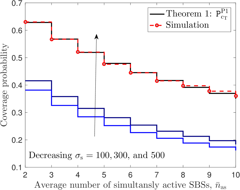
Figure 2: Coverage probability as a function of average number of simultaneously active SBSs for different value of $\sigma_{\rm s}$ under association Policy 1 ($n_{{\rm s}_{0}}=10$ and $\sigma_{\rm s}=\sigma_{\rm u}$)

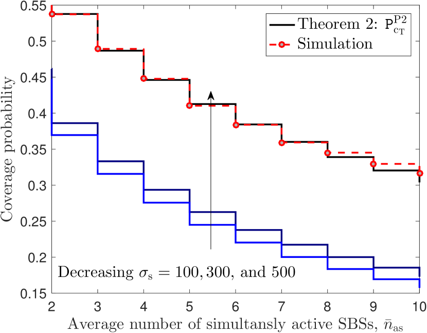
Figure 3: Coverage probability as a function of average number of simultaneously active SBSs for different value of $\sigma_{\rm s}$ under association Policy 2 ($n_{{\rm s}_{0}}=10$ and $\sigma_{\rm s}=\sigma_{\rm u}$)

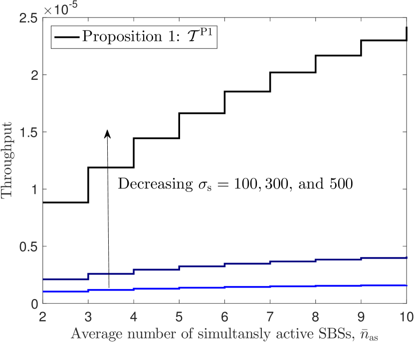
Figure 4: Throughput as a function of average number of simultaneously active SBSs for different value of $\sigma_{\rm s}$ under association Policy 1 ($n_{{\rm s}_{0}}=10$ and $\sigma_{\rm s}=\sigma_{\rm u}$)

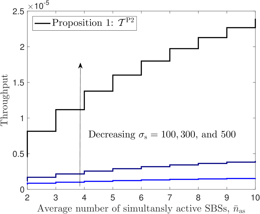
Figure 5: Throughput as a function of average number of simultaneously active SBSs for different value of $\sigma_{\rm s}$ under association Policy 2 ($n_{{\rm s}_{0}}=10$ and $\sigma_{\rm s}=\sigma_{\rm u}$)

V-B Number of simultaneously active SBSs

The coverage probabilities as a function of average number of simultaneously active SBSs, $\bar{n}_{\rm as}$, are presented in Figs. 3 and 3 for association policies 1 and 2. Our analysis concretely demonstrates that the coverage probability always decreases when more SBSs per cluster reuse the same spectrum. This is because having more simultaneously active SBSs results in more interference. However, there is a classical trade-off between frequency reuse and resulting interference. To study this trade-off, we plot throughput as a function of $\bar{n}_{\rm as}$ in Figs. 5 and 5. Interestingly in the considered range, throughput increases with the average number of simultaneously active SBSs per cluster. This means that more and more SBSs can be simultaneously activated as long as the coverage probability remains acceptable. From this observation, it can also be deduced that strictly orthogonal channelization (at most one SBS is allowed to use a given time-frequency resource element/block per cluster) is not spectrally efficient.

V-C Impact of SBS standard deviation

For association Policy 1, the coverage probability as a function of scattering standard deviation of SBSs, $\sigma_{\rm s}$, is plotted in Fig. 7. The plot shows that $\sigma_{\rm s}$ has a conflicting effect on ${\tt P}_{{\rm c}_{\rm m}}^{\rm P1}$ and ${\tt P}_{{\rm c}_{\rm s}}^{\rm P1}$: ${\tt P}_{{\rm c}_{\rm m}}^{\rm P1}$ increases and ${\tt P}_{{\rm c}_{\rm s}}^{\rm P1}$ decreases. The intuition behind this observation is that by increasing $\sigma_{\rm s}$ the association to macrocell increases while association to small cell decreases. In Fig. 7, we plot average association probability as a function of $\sigma_{\rm s}$ to exhibit this trend. From Fig. 9, a similar observation can be made for association Policy 2, where ${\tt P}_{{\rm c}_{\rm m}}^{\rm P2}$ increases and ${\tt P}_{{\rm c}_{\rm s}}^{\rm P2}$ decreases as scattering standard deviation of SBSs increases.

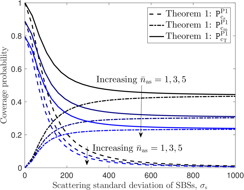
Figure 6: Coverage probability as a function of standard deviation $\sigma_{\rm s}$ for different value of $\bar{n}_{\rm as}$ ($n_{{\rm s}_{0}}=10$ and $\sigma_{\rm s}=\sigma_{\rm u}$)

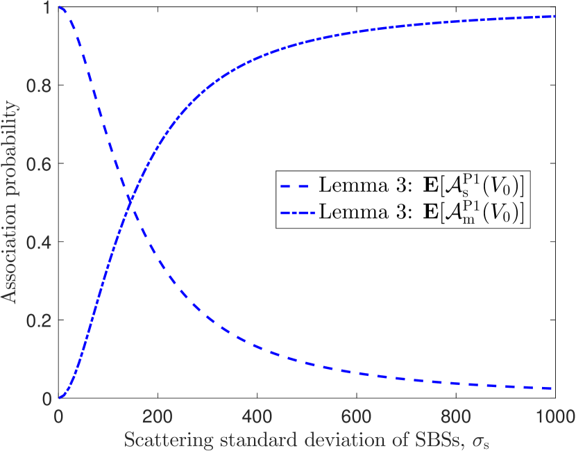
Figure 7: Association probability as a function of standard deviation $\sigma_{\rm s}$ ($n_{{\rm s}_{0}}=10$ and $\sigma_{\rm s}=\sigma_{\rm u}$)

V-D Optimal distance threshold

As evident from Figs. 9 and 9, there exists an optimal SBS power threshold (or equivalently distance threshold $D\equiv\big{(}\frac{P_{\rm 0}}{P_{\rm s}}\big{)}^{-1/\alpha}$) that maximizes the total coverage probability. The existence of the optimal value can be intuitively justified by the conflicting effect of the power threshold on the association to macrocell and small cell, as discussed in Remark 3. From Fig. 9, we can observe that the optimal distance threshold decreases with the increase of average number of simultaneously active SBSs per cluster. This is because although both ${\tt P}_{{\rm c}_{\rm s}}^{\rm P2}$ and ${\tt P}_{{\rm c}_{\rm m}}^{\rm P2}$ decrease with the increase of $\bar{n}_{\rm as}$, the former decreases at a slightly higher rate. Thus it is desirable to associate less users to SBSs. Interestingly, we notice that the optimal distance threshold for different values of $\sigma_{\rm s}$ does not change in the setup considered in Fig. 9.

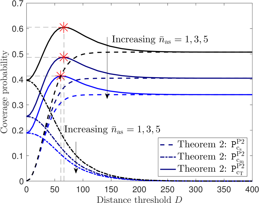
Figure 8: Coverage probability as a function of  $D\equiv\Big{(}\frac{P_{\rm 0}}{P_{\rm s}}\Big{)}^{-1/\alpha}$ for different value of $\bar{n}_{\rm as}$ ($n_{{\rm s}_{0}}=10$ and $\sigma_{\rm s}=\sigma_{\rm u}$)

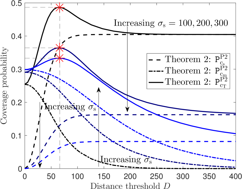
Figure 9: Coverage probability as a function of $D\equiv\Big{(}\frac{P_{\rm 0}}{P_{\rm s}}\Big{)}^{-1/\alpha}$ for different value of $\sigma_{\rm s}$ ($n_{{\rm s}_{0}}=10$ and $\sigma_{\rm s}=\sigma_{\rm u}$).

VI Concluding Remarks

We developed a comprehensive framework for the performance analysis of HetNets with user-centric capacity-driven small cell deployments. Unlike the prior art on the spatial modeling of HetNets where users and SBSs are usually modeled by independent homogeneous PPPs, we introduced a tractable approach to incorporate coupling in the locations of the users and SBSs in HetNets, which bridges the gap between the simulation models used by industry (especially for the user hotspots), such as by 3GPP [2], and the ones used thus far by the stochastic geometry community. In particular, we assumed that the geographical centers of user hotspots are distributed according to a homogeneous PPP around which users and SBSs are located with two general distributions. This approach not only models the aforementioned coupling, but also captures the non-homogeneous nature of user distributions [2]. For this setup, we derived the coverage probability of a typical user and throughput of the whole network for two received power-based association policies. Our setup is general and applicable to any distributions of the relative locations of the users and SBSs with respect to the cluster center. A key intermediate step is the derivation of a new set of distance distributions, which enabled the accurate analysis of user-centric small cell deployments. For numerical evaluation, we considered the special case of Thomas cluster process, which led to several design insights. The most important one is that the throughput increases with the increase of the number of SBSs per cluster reusing the same resource block in the considered setup. Therefore, the usual assumption of strictly orthogonal channelization per cluster should be revisited for efficient design, planning, and dimensioning of the system. The proposed approach has numerous extensions. From modeling perspective, it is desirable to develop a unified analytical model to encompass different spatial configurations considered by 3GPP for modeling BS and user locations in HetNets [60]. Further, it is desirable to choose point process models that simultaneously capture the spatial separation between the macro BSs and SBSs as well as the clustering nature of the SBSs [61]. From analysis perspective, it is important to extend the results to more general channel models, such as $\kappa-\mu$ shadowed fading channels [62], and correlated shadowing. From application perspective, the results can be extended to the analysis of cache enabled network to study metrics like total hit probability and caching throughput; see [63, 48]. Finally, this framework can be extended to the analysis of other key performance metrics such as ergodic spectral efficiency [64] and bit error rate.

-A Proof of Lemma 1

Let us denote the location of SBS chosen uniformly at random in the representative cluster by ${\bf z}_{0}={\bf x}_{0}+{\bf y}_{\rm s}\in\mathbb{R}^{2}$, where ${\bf z}_{0}=(z_{1},z_{2})$ and ${\bf x}_{0}=(\nu_{0},0)$. The conditional CDF of distance $U$ with realization $u=\sqrt{z_{1}^{2}+z_{2}^{2}}\in\mathbb{R}_{+}$ is:

$$F_{U}(u|{\bf x}_{0})=F_{U}(u|\nu_{0}) =\int\int_{\sqrt{z_{1}^{2}+z_{2}^{2}}\leq u}f_{{\bf Y}_{\rm s}}\big{(}z_{1}-\nu_{0},z_{2}\big{)}{\rm d}z_{2}{\rm d}z_{1}$$

$$=\int_{z_{1}=-u}^{z_{1}=u}\int_{z_{2}=-\sqrt{u^{2}-z_{1}^{2}}}^{z_{2}=\sqrt{u^{2}-z_{1}^{2}}}f_{{\bf Y}_{\rm s}}\big{(}z_{1}-\nu_{0},z_{2}\big{)}{\rm d}z_{2}{\rm d}z_{1},$$

where the PDF of $U$ is obtained by using Leibniz’s rule for differentiation [65]. Now recall that the typical user is located at the origin, and users are distributed around cluster center with PDF $f_{{\bf Y}_{\rm u}}({\bf y_{u}})$. Thus, the relative location of the cluster center with respect to the typical user, i.e ${\rm x}_{0}$, has the same distribution as that of ${\bf Y}_{\rm u}$. The PDF of $V_{0}=\|{\bf Y}_{u}\|$ can be derived by using the same argument applied in the derivation of $f_{U}(.)$.

-B Proof of Lemma 3

The conditional association probability to the macro-tier for a given value of $\nu_{0}$ is:

$${\cal A}_{\rm m}^{\rm P1}(\nu_{0}) =\mathbb{E}_{R_{\rm m}}[{\bf 1}\{P_{\rm m}R_{\rm m}^{-\alpha}>P_{\rm s}R_{\rm s}^{-\alpha}\}|\nu_{0}]=\int_{0}^{\infty}\mathbb{P}\Big{[}R_{\rm s}>\big{(}\frac{P_{\rm s}}{P_{\rm m}}\big{)}^{1/\alpha}r_{\rm m}|\nu_{0}\Big{]}f_{R_{\rm m}}(r_{\rm m}){\rm d}r_{\rm m},$$

$$=\int_{0}^{\infty}\Big{[}1-F_{R_{\rm s}}\big{(}\big{(}\frac{P_{\rm s}}{P_{\rm m}}\big{)}^{1/\alpha}r_{\rm m}|\nu_{0}\big{)}\Big{]}f_{R_{\rm m}}(r_{\rm m}){\rm d}r_{\rm m},$$

using which the association probability to the small cell tier is ${\cal A}^{\rm P1}_{\rm s}(\nu_{0})=1-{\cal A}^{\rm P1}_{\rm m}(\nu_{0}).$

-C Proof of Lemma 4

For a given typical user located at distance $\nu_{0}$ from its cluster center, the event $X_{\rm m}^{\rm P1}>x_{\rm m}$ is equivalent to that of $R_{\rm m}>x_{\rm m}$ when the typical user connects to the macro BS, i.e., event $S_{{\rm m}}^{\rm P1}$. Thus, the conditional CCDF of $X_{\rm m}^{\rm P1}$ can be derived as:

$$\mathbb{P}({X_{\rm m}^{\rm P1}>x_{\rm m}}|\nu_{0}) =\mathbb{P}(R_{\rm m}>x_{\rm m}|S_{{\rm m}}^{\rm P1},\nu_{0})=\frac{\mathbb{P}[R_{\rm m}>x_{\rm m},S_{{\rm m}}^{\rm P1}|\nu_{0}]}{\mathbb{P}[S_{{\rm m}}^{\rm P1}|\nu_{0}]}$$ (46)

$$=\frac{1}{{\cal A}_{\rm m}^{\rm P1}(\nu_{0})}\int_{x_{\rm m}}^{\infty}\mathbb{P}(R_{\rm s}>\xi_{\rm sm}\>r_{\rm m}|\nu_{0})f_{R_{\rm m}}(r_{\rm m}){\rm d}{r_{\rm m}},$$ (47)

and hence the PDF of $X_{\rm m}^{\rm P1}$ is:

$$f_{X_{\rm m}^{\rm P1}}(x_{\rm m}|\nu_{0})=\frac{{\rm d}}{{\rm d}x_{\rm m}}(1-\mathbb{P}(X_{\rm m}^{\rm P1}>x_{\rm m}|\nu_{0}))=\frac{1}{{\cal A}_{\rm m}^{\rm P1}(\nu_{0})}(1-F_{R_{\rm s}}(\xi_{\rm sm}x_{\rm m}|\nu_{0}))f_{R_{\rm m}}(x_{\rm m}).$$ (48)

The derivation of $f_{X_{\rm s}^{\rm P1}}(\cdot|\nu_{0})$ follows on the same lines as that of $f_{X_{\rm m}^{\rm P1}}(\cdot|\nu_{0})$, and is hence skipped.

-D Proof of Lemma 5

Denote by $\{U_{j}\}_{j=1}^{n_{{\rm s}_{0}}}$ the sequence of distances from open access SBSs to the typical user. From association Policy 1, it can be deduced that there are no open-access BSs within distance $\xi_{\rm sm}x_{\rm m}$ of the typical user when this user is served by the macro BS. Thus, the sequence of distances from interfering open-access SBSs to the typical user can be defined as ${\cal F}^{\rm P1}_{\rm m}\equiv\{W^{\rm P1}_{{\rm m},j}:W^{\rm P1}_{{\rm m},j}=U_{j},U_{j}>\xi_{\rm sm}x_{\rm m}\}$. The conditional joint density function of the elements in ${\cal F}^{\rm P1}_{\rm m}$ is:

$$\mathbb{P}(W^{\rm P1}_{{\rm m},1}<w_{{\rm m},1},...,W^{\rm P1}_{{\rm m},n_{{\rm s}_{0}}}<w_{{\rm m},n_{{\rm s}_{0}}}|V_{0}=\nu_{0})$$

$$= \mathbb{P}(U_{1}<w_{{\rm m},1},...,U_{n_{{\rm s}_{0}}}<w_{{\rm m},n_{{\rm s}_{0}}}|U_{1}>\xi_{\rm sm}x_{\rm m},...,U_{n_{\rm s}}>\xi_{\rm sm}x_{\rm m},V_{0}=\nu_{0})$$

$$= \left\{\begin{array}[]{cc}\frac{\mathbb{P}(U_{1}<w_{{\rm m},1},...,U_{n_{{\rm s}_{0}}}<w_{{\rm m},n_{{\rm s}_{0}}}|V_{0}=\nu_{0})}{\mathbb{P}(U_{1}>\xi_{\rm sm}x_{\rm m},...,U_{n_{\rm s}}>\xi_{\rm sm}x_{\rm m}|V_{0}=\nu_{0})},&w_{{\rm m},j}\geq\xi_{\rm sm}x_{\rm m}\\ 0,&0\leq w_{{\rm m},j}<\xi_{\rm sm}x_{\rm m}\end{array}\right.,\quad j=\{1,2,...,n_{{\rm s}_{0}}\}$$

$$\stackrel{{\scriptstyle(a)}}{{=}} \left\{\begin{array}[]{cc}\prod_{j=1}^{n_{{\rm s}_{0}}}\frac{F_{U_{j}}(w_{{\rm m},j}|\nu_{0})}{1-F_{U_{j}}(\xi_{\rm sm}x_{\rm m}|\nu_{0})},&w_{{\rm m},j}\geq\xi_{\rm sm}x_{\rm m}\\ 0,&0\leq w_{{\rm m},j}<\xi_{\rm sm}x_{\rm m}\end{array}\right.,\quad j=\{1,2,...,n_{{\rm s}_{0}}\},$$

where $(a)$ follows from the fact that the elements in $\{U_{j}\}_{j=1}^{n_{{\rm s}_{0}}}$ are conditionally i.i.d. (see Lemma 1). The product of the same functional form in the joint CDF implies that the elements in ${\cal F}^{\rm P1}_{\rm m}$ are conditionally i.i.d. with CDF $F_{W^{\rm P1}_{{\rm m},j}}(w_{{\rm m},j}|\nu_{0},x_{\rm m})=\frac{F_{U_{j}}(w_{{\rm m},j}|\nu_{0})}{1-F_{U_{j}}(\xi_{\rm sm}x_{\rm m}|\nu_{0})}$. Using this result, the PDF of $W^{\rm P1}_{{\rm m},j}$ can be obtained by taking derivative of $F_{W^{\rm P1}_{{\rm m},j}}(w_{{\rm m},j}|\nu_{0},x_{\rm m})$ with respect to $w_{{\rm m},j}$. In the final result, index $j$ is dropped for notational simplicity. The derivation of $f_{W^{\rm P1}_{{\rm s}}}(\cdot|\nu_{0},x_{\rm s})$ follows on the same lines as that of ${W^{\rm P1}_{{\rm m}}}$, and is hence skipped.

-E Proof of Lemma 9

The Laplace transform of intra-cluster interference distribution at a typical user served by macrocell conditioned on $V_{0}$ and $X^{\rm P1}_{\rm m}$ is:

$${\cal L}_{{\cal I}_{\rm sm}^{\rm intra}}(s|\nu_{0},x_{\rm m})\stackrel{{\scriptstyle(a)}}{{=}}\mathbb{E}\Big{[}\exp\Big{(}-s\sum_{{\bf y}_{\rm s}\in{\cal B}_{\rm s}^{{\bf x}_{0}}}P_{\rm s}h_{\rm s}\|{\bf x}_{0}+{\bf y}_{\rm s}\|^{-\alpha}\Big{)}\Big{]}\stackrel{{\scriptstyle(b)}}{{=}}\mathbb{E}\Big{[}\prod_{{\bf y}_{\rm s}\in{\cal B}_{\rm s}^{{\bf x}_{0}}}\frac{1}{1+sP_{\rm s}\|{\bf x}_{0}+{\bf y}_{\rm s}\|^{-\alpha}}\Big{]},$$

where $(a)$ follows from the definition of Laplace transform and $(b)$ follows from the expectation over $h_{\rm s}\sim\exp(1)$. The final result follows from the change of variable $\|{\bf x}_{0}+{\bf y}_{\rm s}\|\rightarrow w_{\rm m}$, and converting from Cartesian to polar coordinates, followed by the fact that the elements of $\{W_{\rm m}\}$ are conditionally i.i.d., with PDF $f_{W^{\rm P1}_{\rm m}}(w_{\rm m}|\nu_{0},x_{\rm m})$ given by Lemma 5, followed by expectation over the number of simultaneously active SBSs within the representative cluster with PDF

$$\mathbb{P}(|{\cal B}_{\rm s}^{{\bf x}_{0}}|=\ell)=\frac{{\bar{n}_{\rm as}}^{\ell}e^{-\bar{n}_{\rm as}}}{\ell!\sum_{k=0}^{n_{\rm s_{0}}}\frac{{\bar{n}_{\rm as}}^{k}e^{-\bar{n}_{\rm as}}}{k!}},\quad 0\leq\ell\leq n_{{\rm s_{0}}},$$ (49)

where $|{\cal B}_{\rm s}^{{\bf x}_{0}}|$ is Poisson distributed conditioned on the total being less than $n_{\rm s_{0}}$. The derivation of ${\cal L}_{{\cal I}_{\rm ss}^{\rm intra}}(.|\nu_{0},x_{\rm s})$ follows on the same lines as that of ${\cal L}_{{\cal I}_{\rm sm}^{\rm intra}}(.|\nu_{0},x_{\rm m})$, where the serving SBS is removed from the set of possible interfering SBSs. The PDF of number of simultaneously active SBSs within the representative cluster $|{\cal B}_{\rm s}^{{\bf x}_{0}}|$ conditioned on having at least one active SBS (serving SBS) is:

$$\mathbb{P}(|{\cal B}_{\rm s}^{{\bf x}_{0}}|=\ell)=\frac{{\bar{n}_{\rm as}}^{\ell-1}e^{-\bar{n}_{\rm as}}}{(\ell-1)!\sum_{k=1}^{n_{\rm s_{0}}}\frac{{\bar{n}_{\rm as}}^{k-1}e^{-\bar{n}_{\rm as}}}{(k-1)!}},\quad 1\leq\ell\leq n_{{\rm s_{0}}},$$ (50)

which is truncated weighted Poisson distribution.

-F Proof of Lemma 10

Note that the Laplace transform of inter-cluster interference does not depend on the choice of the serving BS. Denoting by $j\in\{{\rm s},{\rm m}\}$ the index of the serving BS, the Laplace transform of inter-cluster interference ${\cal I}^{\rm inter}_{{\rm s}j}$ is ${\cal L}_{{\cal I}^{\rm inter}_{{\rm s}j}}(s)$

$$\stackrel{{\scriptstyle(a)}}{{=}}\mathbb{E}\Big{[}\exp\Big{(}-s\sum_{{\bf x}\in\Psi_{\rm p}\setminus{\bf x}_{0}}\sum_{{\bf y}_{\rm s}\in{\cal B}_{\rm s}^{{\bf x}}}P_{\rm s}h_{\rm s}\|{\bf x}+{\bf y}_{\rm s}\|^{-\alpha}\Big{)}\Big{]}$$

$$\stackrel{{\scriptstyle(b)}}{{=}}\mathbb{E}_{\Psi_{\rm p}}\prod_{{\bf x}\in\Psi_{\rm p}\setminus{\bf x}_{0}}\mathbb{E}_{{\cal B}_{\rm s}^{{\bf x}}}\prod_{{\bf y}_{\rm s}\in{\cal B}_{\rm s}^{{\bf x}}}\mathbb{E}_{h_{\rm s}}\exp\Big{(}-sP_{\rm s}h_{\rm s}\|{\bf x}+{\bf y}_{\rm s}\|^{-\alpha}\Big{)}$$

$$\stackrel{{\scriptstyle(c)}}{{=}}\mathbb{E}_{\Psi_{\rm p}}\prod_{{\bf x}\in\Psi_{\rm p}\setminus{\bf x}_{0}}\mathbb{E}_{{\cal B}_{\rm s}^{{\bf x}}}\prod_{{\bf y}_{\rm s}\in{\cal B}_{\rm s}^{{\bf x}}}\frac{1}{1+sP_{\rm s}\|{\bf x}+{\bf y}_{\rm s}\|^{-\alpha}}$$

$$\stackrel{{\scriptstyle(d)}}{{=}}\mathbb{E}_{\Psi_{\rm p}}\prod_{{\bf x}\in\Psi_{\rm p}\setminus{\bf x}_{0}}\exp\Big{(}-\bar{n}_{\rm as}\int_{0}^{\infty}\frac{sP_{\rm s}t_{\rm s}^{-\alpha}}{1+sP_{\rm s}t_{\rm s}^{-\alpha}}f_{T_{\rm s}}(t_{\rm s}|\nu){\rm d}{t_{\rm s}}\Big{)}$$

$$\stackrel{{\scriptstyle(e)}}{{=}}\exp\Big{(}-2\pi\lambda_{\rm p}\int_{0}^{\infty}\Big{(}1-\exp\Big{(}-\bar{n}_{\rm as}\int_{0}^{\infty}\frac{sP_{\rm s}t_{\rm s}^{-\alpha}}{1+sP_{\rm s}t_{\rm s}^{-\alpha}}f_{T_{\rm s}}(t_{\rm s}|\nu){\rm d}{t_{\rm s}}\Big{)}\Big{)}\nu{\rm d}{\nu}\Big{)},$$

where $(a)$ follows from definition of Laplace transform, $(b)$ follow from the assumption that fading gains across all interfering links are independent, $(c)$ follows from the expectation over $h_{\rm s}\sim\exp(1)$, $(d)$ follows from the change of variable $\|{\bf x}_{0}+{\bf y}_{\rm s}\|\rightarrow t_{\rm s}$, and converting from Cartesian to polar coordinates, followed by the fact that number of points per cluster are Poisson distributed, and $(e)$ follows from probability generating functional (PGFL) of PPP.

References

• [1] M. Afshang and H. S. Dhillon, “A new clustered HetNet model to accurately characterize user-centric small cell deployments,” in Proc. IEEE WCNC, Mar. 2016.
• [2] 3GPP TR 36.814, “Further advancements for E-UTRA physical layer aspects,” Tech. Rep., 2010.
• [3] 3GPP, “Consideration of UE Cluster Position and PeNB TX Power in Heterogeneous Deployment Configuration 4,” Discussion/ Decision R1-100477.
• [4] V. Chandrasekhar, J. G. Andrews, and A. Gatherer, “Femtocell networks: a survey,” IEEE Commun. Magazine, vol. 46, no. 9, pp. 59–67, Sep. 2008.
• [5] A. Damnjanovic, J. Montojo, Y. Wei, T. Ji, T. Luo, M. Vajapeyam, T. Yoo, O. Song, and D. Malladi, “A survey on 3GPP heterogeneous networks,” IEEE Wireless Commun. Magazine, vol. 18, no. 3, pp. 10–21, Jun. 2011.
• [6] J. G. Andrews, “Seven ways that HetNets are a cellular paradigm shift,” IEEE Commun. Magazine, vol. 51, no. 3, pp. 136–144, Mar. 2013.
• [7] M. Mirahsan, R. Schoenen, and H. Yanikomeroglu, “HetHetNets: Heterogeneous traffic distribution in heterogeneous wireless cellular networks,” IEEE Journal on Sel. Areas in Commun., vol. 33, no. 10, pp. 2252–2265, Oct. 2015.
• [8] S. Mukherjee, Analytical Modeling of Heterogeneous Cellular Networks.   Cambridge University Press, 2014.
• [9] H. Elsawy, E. Hossain, and M. Haenggi, “Stochastic geometry for modeling, analysis, and design of multi-tier and cognitive cellular wireless networks: A survey,” IEEE Commun. Surveys and Tutorials, vol. 15, no. 3, pp. 996–1019, 3th quarter 2013.
• [10] J. G. Andrews, A. K. Gupta, and H. S. Dhillon, “A primer on cellular network analysis using stochastic geometry,” arXiv preprint, 2016, available online: arxiv.org/abs/1604.03183.
• [11] H. ElSawy, A. Sultan-Salem, M. S. Alouini, and M. Z. Win, “Modeling and analysis of cellular networks using stochastic geometry: A tutorial,” IEEE Commun. Surveys and Tutorials, vol. 19, no. 1, pp. 167–203, Firstquarter 2017.
• [12] H. S. Dhillon, R. K. Ganti, F. Baccelli, and J. G. Andrews, “Modeling and analysis of $K$-tier downlink heterogeneous cellular networks,” IEEE Journal on Sel. Areas in Commun., vol. 30, no. 3, pp. 550–560, Apr. 2012.
• [13] H. S. Dhillon, R. K. Ganti, and J. G. Andrews, “A tractable framework for coverage and outage in heterogeneous cellular networks,” in Proc., Information Theory and Applications Workshop (ITA), Feb. 2011.
• [14] J. G. Andrews, F. Baccelli, and R. K. Ganti, “A tractable approach to coverage and rate in cellular networks,” IEEE Trans. on Commun., vol. 59, no. 11, pp. 3122–3134, Nov. 2011.
• [15] M. D. Renzo and W. Lu, “Stochastic geometry modeling and performance evaluation of MIMO cellular networks using the equivalent-in-distribution (EiD)-based approach,” IEEE Trans. on Commun., vol. 63, no. 3, pp. 977–996, Mar. 2015.
• [16] S. Mukherjee, “Distribution of downlink SINR in heterogeneous cellular networks,” IEEE Journal on Sel. Areas in Commun., vol. 30, no. 3, pp. 575–585, Apr. 2012.
• [17] H.-S. Jo, Y. J. Sang, P. Xia, and J. G. Andrews, “Heterogeneous cellular networks with flexible cell association: A comprehensive downlink SINR analysis,” IEEE Trans. on Wireless Commun., vol. 11, no. 10, pp. 3484–3495, Oct. 2012.
• [18] P. Madhusudhanan, J. G. Restrepo, Y. Liu, T. X. Brown, and K. R. Baker, “Downlink performance analysis for a generalized shotgun cellular system,” IEEE Trans. on Wireless Commun., vol. 13, no. 12, pp. 6684–6696, Dec. 2014.
• [19] R. Tanbourgi, S. Singh, J. G. Andrews, and F. K. Jondral, “A tractable model for noncoherent joint-transmission base station cooperation,” IEEE Trans. on Wireless Commun., vol. 13, no. 9, pp. 4959–4973, Sep. 2014.
• [20] G. Nigam, P. Minero, and M. Haenggi, “Coordinated multipoint joint transmission in heterogeneous networks,” IEEE Trans. on Commun., vol. 62, no. 11, pp. 4134–4146, Nov. 2014.
• [21] A. H. Sakr and E. Hossain, “Location-aware cross-tier coordinated multipoint transmission in two-tier cellular networks,” IEEE Trans. on Wireless Commun., vol. 13, no. 11, pp. 6311–6325, Nov. 2014.
• [22] R. W. Heath, M. Kountouris, and T. Bai, “Modeling heterogeneous network interference using Poisson point processes,” IEEE Trans. on Signal Processing, vol. 61, no. 16, pp. 4114–4126, Aug. 2013.
• [23] S. Singh, H. S. Dhillon, and J. G. Andrews, “Offloading in heterogeneous networks: Modeling, analysis, and design insights,” IEEE Trans. on Wireless Commun., vol. 12, no. 5, pp. 2484–2497, May. 2013.
• [24] H. S. Dhillon and J. G. Andrews, “Downlink rate distribution in heterogeneous cellular networks under generalized cell selection,” IEEE Wireless Commun. Letters, vol. 3, no. 1, pp. 42–45, Feb. 2014.
• [25] A. K. Gupta, H. S. Dhillon, S. Vishwanath, and J. G. Andrews, “Downlink multi-antenna heterogeneous cellular network with load balancing,” IEEE Trans. on Commun., vol. 62, no. 11, pp. 4052–4067, Nov. 2014.
• [26] Y. S. Soh, T. Q. S. Quek, M. Kountouris, and H. Shin, “Energy efficient heterogeneous cellular networks,” IEEE Journal on Sel. Areas in Commun., vol. 31, no. 5, pp. 840–850, May 2013.
• [27] M. D. Renzo, A. Guidotti, and G. E. Corazza, “Average rate of downlink heterogeneous cellular networks over generalized fading channels: A stochastic geometry approach,” IEEE Trans. on Commun., vol. 61, no. 7, pp. 3050–3071, Jul. 2013.
• [28] W. C. Cheung, T. Q. S. Quek, and M. Kountouris, “Throughput optimization, spectrum allocation, and access control in two-tier femtocell networks,” IEEE Journal on Sel. Areas in Commun., vol. 30, no. 3, pp. 561–574, Apr. 2012.
• [29] H. S. Dhillon, Y. Li, P. Nuggehalli, Z. Pi, and J. G. Andrews, “Fundamentals of heterogeneous cellular networks with energy harvesting,” IEEE Trans. on Wireless Commun., vol. 13, no. 5, pp. 2782–2797, May. 2014.
• [30] H. S. Dhillon, M. Kountouris, and J. G. Andrews, “Downlink MIMO HetNets: Modeling, ordering results and performance analysis,” IEEE Trans. on Wireless Commun., vol. 12, no. 10, pp. 5208–5222, Oct. 2013.
• [31] C. Li, J. Zhang, and K. B. Letaief, “Throughput and energy efficiency analysis of small cell networks with multi-antenna base stations,” IEEE Trans. on Wireless Commun., vol. 13, no. 5, pp. 2505–2517, May 2014.
• [32] C. Li, J. Zhang, J. G. Andrews, and K. B. Letaief, “Success probability and area spectral efficiency in multiuser MIMO HetNets,” IEEE Trans. on Commun., vol. 64, no. 4, pp. 1544–1556, Apr. 2016.
• [33] M. D. Renzo and P. Guan, “A mathematical framework to the computation of the error probability of downlink MIMO cellular networks by using stochastic geometry,” IEEE Trans. on Commun., vol. 62, no. 8, pp. 2860–2879, Aug. 2014.
• [34] F. Baccelli and A. Giovanidis, “A stochastic geometry framework for analyzing pairwise-cooperative cellular networks,” IEEE Trans. on Wireless Commun., vol. 14, no. 2, pp. 794–808, Feb. 2015.
• [35] H. S. Dhillon, R. K. Ganti, and J. G. Andrews, “Modeling non-uniform UE distributions in downlink cellular networks,” IEEE Wireless Commun. Letters, vol. 2, no. 3, pp. 339–342, Jun. 2013.
• [36] M. Afshang, H. S. Dhillon, and P. H. J. Chong, “Modeling and performance analysis of clustered device-to-device networks,” IEEE Trans. on Wireless Commun., vol. 15, no. 7, pp. 4957–4972, Jul. 2016.
• [37] ——, “Fundamentals of cluster-centric content placement in cache-enabled device-to-device networks,” IEEE Trans. on Commun., vol. 64, no. 6, pp. 2511–2526, Jun. 2016.
• [38] M. Afshang and H. S. Dhillon, “Fundamentals of modeling finite wireless networks using binomial point process,” IEEE Trans. on Wireless Commun., 2017, to appear.
• [39] M. Afshang, C. Saha, and H. S. Dhillon, “Nearest-neighbor and contact distance distributions for Thomas cluster process,” IEEE Wireless Commun. Letters, vol. 6, no. 1, pp. 130–133, Feb. 2017.
• [40] C. Saha and H. S. Dhillon, “Downlink coverage probability of $K$-tier HetNets with general non-uniformuser distributions,” in Proc., IEEE Intl. Conf. on Commun. (ICC), May 2016.
• [41] C. Saha, M. Afshang, and H. S. Dhillon, “Enriched $K$-tier HetNet model to enable the analysis of user-centric small cell deployments,” IEEE Trans. on Wireless Commun., vol. 16, no. 3, pp. 1593–1608, Mar. 2017.
• [42] H.Tabassum, E. Hossain, and M. J. Hossain, “Modeling and analysis of uplink non-orthogonal multiple access (NOMA) in large-scale cellular networks using Poisson cluster processes,” arXiv preprint, 2016, available online: arxiv.org/abs/1610.06995.
• [43] P. D. Mankar, G. Das, and S. S. Pathak, “Modeling and coverage analysis of BS-centric clustered users in a random wireless network,” IEEE Wireless Commun. Letters, vol. 5, no. 2, pp. 208–211, Apr. 2016.
• [44] J. G. Andrews, R. K. Ganti, M. Haenggi, N. Jindal, and S. Weber, “A primer on spatial modeling and analysis in wireless networks,” IEEE Commun. Magazine, vol. 48, no. 11, pp. 156–163, Nov. 2010.
• [45] C.-H. Lee, C.-Y. Shih, and Y.-S. Chen, “Stochastic geometry based models for modeling cellular networks in urban areas,” Wireless networks, vol. 19, no. 6, pp. 1063–1072, Oct 2013.
• [46] Y. Zhong and W. Zhang, “Multi-channel hybrid access femtocells: A stochastic geometric analysis,” IEEE Trans. on Commun., vol. 61, no. 7, pp. 3016–3026, Jul. 2013.
• [47] Y. J. Chun, M. O. Hasna, and A. Ghrayeb, “Modeling heterogeneous cellular networks interference using Poisson cluster processes,” IEEE Journal on Sel. Areas in Commun., vol. 33, no. 10, pp. 2182–2195, Oct. 2015.
• [48] E. Baştuğ, M. Bennis, M. Kountouris, and M. Debbah, “Edge caching for coverage and capacity-aided heterogeneous networks,” in Proc., IEEE International Symposium on Information Theory (ISIT), Jul. 2016.
• [49] Y. Wang and Q. Zhu, “Modeling and analysis of small cells based on clustered stochastic geometry,” IEEE Commun. Letters, 2016, to appear.
• [50] V. Suryaprakash, J. Møller, and G. Fettweis, “On the modeling and analysis of heterogeneous radio access networks using a Poisson cluster process,” IEEE Trans. on Wireless Commun., vol. 14, no. 2, pp. 1035–1047, Feb. 2015.
• [51] C. Chen, R. C. Elliott, and W. A. Krzymien, “Downlink coverage analysis of n-tier heterogeneous cellular networks based on clustered stochastic geometry,” in Proc., IEEE Asilomar, Nov. 2013, pp. 1577–1581.
• [52] P. D. Mankar, G. Das, and S. Pathak, “Coverage analysis of two-tier HetNets for co-channel, orthogonal, and partial spectrum sharing under fractional load conditions,” IEEE Trans. on Vehicular Technology, 2017, to appear.
• [53] N. Deng, W. Zhou, and M. Haenggi, “Heterogeneous cellular network models with dependence,” IEEE Journal on Sel. Areas in Commun., vol. 33, no. 10, pp. 2167–2181, Oct. 2015.
• [54] D. J. Daley and D. Vere-Jones, An Introduction to the Theory of Point Processes. Volume I: Elementary Theory and Methods, 2nd ed.   New York: Springer-Verlag, 2003.
• [55] R. K. Ganti and M. Haenggi, “Interference and outage in clustered wireless ad hoc networks,” IEEE Trans. on Info. Theory, vol. 55, no. 9, pp. 4067–4086, Sep. 2009.
• [56] M. Haenggi, Stochastic Geometry for Wireless Networks.   Cambridge University Press, 2012.
• [57] ——, “On distances in uniformly random networks,” IEEE Trans. on Info. Theory, vol. 51, no. 10, pp. 3584–3586, Oct. 2005.
• [58] H. A. David and H. N. Nagaraja, Order Statistics.   New York: John Wiley and Sons, 1970.
• [59] D. Zwillinger, Table of integrals, series, and products.   Elsevier, 2014.
• [60] C. Saha, M. Afshang, and H. S. Dhillon, “Poisson cluster process: Bridging the gap between PPP and 3GPP HetNet models,” in Proc., Information Theory and Applications Workshop (ITA), Feb. 2017.
• [61] M. Afshang and H. S. Dhillon, “Spatial modeling of device-to-device networks: Poisson cluster process meets Poisson hole process,” in Proc. Asilomar, Pacific Grove, CA, Nov. 2015.
• [62] Y. J. Chun, S. L. Cotton, H. S. Dhillon, F. J. Lopez-Martinez, J. F. Paris, and S. K. Yoo, “A comprehensive analysis of 5G heterogeneous cellular systems operating over $\kappa$-$\mu$ shadowed fading channels,” submitted to IEEE Trans. on Wireless Commun., Oct. 2016, available online: arxiv.org/abs/1609.09696.
• [63] M. Afshang and H. S. Dhillon, “Optimal geographic caching in finite wireless networks,” in Proc., IEEE SPAWC, Jul. 2016.
• [64] G. George, R. Mungara, A. Lozano, and M. Haenggi, “Ergodic spectral efficiency in MIMO cellular networks,” IEEE Trans. on Wireless Commun., 2017, to appear.
• [65] S. G. Samko, A. A. Kilbas, and O. I. Marichev, Fractional integrals and derivatives: Theory and Applications.   London: Gordon and Breach, 1993.