Dynamic conductivity of one-dimensional ion conductors. Impedance, Nyquist diagrams

Abstract

Dynamic conductivity of the one-dimensional ion conductor is investigated at different values of the interaction constant between particles and the modulating field. The consideration is based on the hard-core boson lattice model. Calculations are performed for finite one-dimensional cluster using the exact diagonalization method. Frequency dependence of the dynamic conductivity and behaviour of its static component (Drude weight) in the charge-density-wave (CDW) and superfluid (SF) phases are studied. Frequency dispersion of impedance and loss tangent is calculated; the Nyquist diagrams are built and analyzed.

Key words: ion conductor, hard-core boson model, Drude weight, dynamic conductivity, Nyquist diagrams

PACS: 75.10.Pq, 03.75.Lm, 66.30.Dn

Abstract

Дослiджено залежнiсть динамiчної провiдностi одновимiрного iонного провiдника в залежностi вiд величини взаємодiї мiж частинками i величини модулюючого поля. Розгляд базується на гратковiй моделi жорстких бозонiв. Розрахунки проведено методом точної дiагоналiзацiї для скiнченного одновимiрного кластера. Вивчається частотна залежнiсть динамiчної провiдностi i поведiнка її статичної складової (внеску Друде) в зарядовпорядкованiй фазi (CDW) i в фазi типу суперфлюїду (SF). Розраховано частотну дисперсiю iмпедансу i тангенса втрат; побудовано дiаграми Найквiста.

Ключовi слова: iонний провiдник, модель жорстких бозонiв, внесок Друде, динамiчна провiднiсть, дiаграми Найквiста

1 Introduction

Transport properties of one-dimensional systems are of great interest over many years [1, 2, 3, 4, 5, 6, 7, 8, 9]. One-dimensional objects have special features, and, in addition, the relevant models are investigated much easier than for higher dimensionalities and in many cases permit to obtain exact solutions. The resulting solutions frequently provide the understanding of conduction for 2d and 3d systems, but, at the same time, there exist purely one-dimensional complex problems. The systems with ionic conductivity are of special interest. Attention to these systems is paid due to ever-increasing possibilities of their practical applications as solid electrolytes in capacitors and batteries, in membranes of fuel cells [10], in electronics, in controlling and signalling devices for special purposes. Therefore, new compounds with high ionic conductivity were recently synthesized in order to find materials stable against chemical and mechanical action and possessing other specific properties. Just recently a new superionic crystal Li₁₀GeP₂S₁₂, the conductivity of which reaches 12 mΩ^-1 cm^-1 at room temperature and 0.41 mΩ^-1 cm^-1 at $-30^{\circ}$C, was synthesized [11]. The conductivity of ionic conductors is especially high when a number of ions is much smaller than the number of positions in a lattice, i.e., when there are vacancies. Therefore, a lot of free positions facilitate the ion hopping probability from one position to another. Charge transfer process in some superionics occurs along the chain (one-dimensional) structures. The proton conductor LiN₂H₅SO₄ [12], some superionic (superprotonic) conductors, in particular CsHSO₄ [13], coordination polymers such as iron oxalate dihydrate Fe(C₂O₄)$\,\cdot\,$2H₂O, nanotubes [14], etc. are the examples. One-dimensional system with Josephson junctions (one contact in width and several hundred tunnel contacts in length) are created [15]. In most cases, the quantum systems are studied at low temperatures, when the transport properties of a system are determined mainly by their ground state. Conductivity at high temperatures is less studied. In such a case one cannot restrict oneself to strictly defined elementary excitations (see for example [9]).

Lattice models are widely used for a theoretical description of ion and proton transport at the microscopic level. As a rule, the Bose-Hubbard model is used here at arbitrary occupation of local particle positions (see review [16]). There are also used the models based on Fermi statistics [17, 18, 19, 20, 21] or on the ‘‘mixed’’ Pauli statistics [1, 22, 23, 24, 25, 26, 27, 28, 29, 30, 31, 32, 33, 34, 35], where particles are of Bose nature, but they obey the Fermi rule as well. The lattice model of Pauli particles is similar to the Bose-Hubbard model in the hard-core approximation (provided that the occupation numbers are restricted, $n_{i}$ = $0,1$). When taking into account only the on-site interaction ($U$) of particles in the one-dimensional Bose-Hubbard model, the Mott insulator (MI) phase with the integer particle density was received. At intermediate concentrations, the superfluid (SF) type state [the phase with the infinitely large (divergent) boson correlation length and without the order parameter (see for example [7])] appears at $T=0$. Inclusion of the near-neighbors interaction ($V$) leads to charge-density-wave phase (CDW) with half-filling of ionic sites on the average. The Pauli (hard-core boson) lattice model also enables one to describe the transitions (which are the true ones only at $T=0$) between these phases, including the emergence of the SF-type state that can appear even in the absence of a direct interaction between particles [22, 23, 25].

In our previous work [24] in the hard-core boson approximation, the one-particle spectral density was calculated. The exact diagonalization method for finite one-dimensional lattice model with periodic boundary conditions was used. The conditions of existence of various phases of a system, depending on the values of interaction between particles $V$ and the modulating field strength $A$, were established by analyzing the character of spectral density; the phase diagrams were built [24]. The results agree with the known ones from the literature. In particular, the diagram of state for the case $V=0$ coincides with the exact diagram obtained analytically for the one-dimensional case, see for example [29] (the exact analytical solution can be obtained in this case by applying the Jordan-Wigner transformation, which makes it possible to pass from the Hamiltonian of hard-core bosons to the Hamiltonian of noninteracting spinless fermions). It was shown in [24] that at $T=0$, the repulsive short-range interaction between particles ($V>0$) results in the emergence of a gap in the energy spectrum in the limit of half-filling ($n=1/2$). A true CDW phase is realized here only at zero temperature. The gap in the CDW-phase spectrum grows if the magnitude of either the short-range interaction $V$ or the modulating field $A$ (which can be associated with an internal field that appears owing to the long-range interaction) increases. At $T\neq 0$, the gap gradually disappears with the temperature rise; the interphase boundaries on the ($T,\,\mu$) plane become smeared, and the corresponding phase transitions in this case reduce to the crossover transformations, i.e., they are not genuine phase transitions.

This work is devoted to the calculation of static and dynamic conductivity of one-dimensional ion conductor. The attention was mostly focused on the study of the static conductivity $\sigma(\omega=0)$ described by the so-called Drude weight $D$ [8, 36, 37, 3, 38, 39]. The value of $D$ usually serves as a criterion that determines the state of a system: superconducting (superfluid), metallic, or dielectric (insulator). For infinite systems $D=0$ in the case of insulator (the MI phase or CDW phase) and $D$ is finite in the case of a conducting state (SF phase). For 1d systems of finite length ($L$), the Drude weight $D$ goes exponentially to zero at $L\rightarrow\infty$ in an insulator state (the phase with a gap in spectrum), but remains finite in this limit in the conducting one (the gapless phase), [3, 38, 39]. The investigations of the frequency dependence of the dynamic part of conductivity $\sigma_{\text{reg}}(\omega)$ in the MI phase show that this quantity is equal to zero at low frequencies and becomes nonzero starting from some threshold value of $\omega$ [2, 39]. Contrary to that, in the SF phase, the $\sigma_{\text{reg}}(\omega)$ function increases with frequency according to the power law starting from the zero value at $\omega=0$ [6] and decreases exponentially at high frequencies. Besides that, the existence of peaks on the frequency dependence of $\sigma_{\text{reg}}(\omega)$ was noticeable. For 1d models with finite on-site repulsion $U$, the presence of three peaks was shown in [7]; the peaks are located in the frequency region $\hbar\omega\sim U$. The calculations, performed in the case of hard-core bosons for MI phase, revealed one (or two, depending on approximation) peak of $\sigma_{\text{reg}}(\omega)$ [40].

Our lattice model includes the ion transfer, the interaction between the neighboring ions, and the modulating field. By applying the exact diagonalization technique we determine the energy spectrum and matrix elements of the current density operator for the finite one-dimensional model of the ionic conductor. Based on the Kubo theory [41], we numerically calculate the static (Drude weight) and dynamic (frequency dependent) parts of conductivity. The main attention is paid to the investigation of the ion conductivity in the SF and CDW phases and to the study of the effect of the short-range interaction between particles as well as the modulating field (that effectively appears due to long-range interaction or due to the two-sublattice structure). Restricting ourselves to the $T=0$ case, we analyze the differences between the Drude weight values and frequency dispersion of conductivity in CDW and SF phases. In addition, the plots of impedance are presented and Nyquist diagrams are built. In our consideration, we restrict ourselves in this work to the case $T=0$.

2 Hamiltonian and its transformation

We consider the one-dimensional ion conductor as the chain of heavy immobile ionic groups and light ions that move along this chain occupying certain positions between the mentioned groups. The subsystem of light ions is described with the following Hamiltonian

$$\hat{H} = t\sum\limits_{i}(c_{i}^{+}c_{i+1}+c_{i+1}^{+}c_{i})+V\sum_{i}n_{i}n_{i+1}-\mu\sum_{i}n_{i}+A\sum_{i}(-1)^{i}n_{i}.$$ (2.1)

Here, the operators of creation and annihilation of particles ($c^{+}_{i,\alpha}$ and $c_{i,\alpha}$) obey the Pauli statistics. The model (2.1) is equivalent to the hard-core boson model. The model takes into account the nearest-neighbour ion transfer (with hopping parameter $t$), interaction between ions that occupy nearest-neighbouring positions (with corresponding parameter $V>0$) and modulating field (parameter $A$). The system is divided into two sublattices under the effect of the $A$ field, which simulates the long-range interactions between the particles, which contributes to the modulation of the spatial distribution of light ions in the so-called ordered phase (the existence of such phases at low temperatures is a characteristic feature of superionic conductors).

In order to calculate the energy spectrum of the one-dimensional ionic Pauli conductor we apply the exact diagonalization technique. For this purpose, let us consider a finite chain with periodic boundary conditions. For a chain with $N$ sites in the main region, we introduce the many-particle states

$$\mid n_{1}\,,n_{2}\,,\ldots,n_{N}\rangle.$$ (2.2)

The Hamiltonian matrix on the basis of these states is the matrix of the order $2^{N}\times 2^{N}$. This matrix is numerically diagonalized [24]. Such an operation corresponds to the transformation

$$U^{-1}HU=\widetilde{H}=\sum\limits_{p}E_{p}\widetilde{X}^{pp},$$ (2.3)

where $E_{p}$ are eigenvalues of the Hamiltonian, $\widetilde{X}^{pp}$ are Hubbard operators. The same transformation is applied to the operators of particle creation and annihilation at the $i$-th chain site

$$U^{-1}c_{i}U=\sum\limits_{p,q}A^{i}_{pq}\widetilde{X}^{pq},\qquad\quad U^{-1}c^{+}_{i}U=\sum\limits_{r,s}A^{i*}_{rs}\widetilde{X}^{rs}.$$ (2.4)

Herein below we shall express the current density and conductivity operators applying this representation. It should be marked that we used it in [24] to calculate the single-particle spectral density $\rho(\omega)=-2\mathop{\symoperators Im}\nolimits\langle\langle c|c^{+}\rangle\rangle$ for the model (2.1) and analyze its form in different phases of the system.

3 Dynamic conductivity. General relations

The dynamic conductivity of one-dimensional ion conductor can be calculated starting from the Kubo formula [41]

$$\sigma(\omega,T)=\int\limits_{-\infty}^{0}\mathrm{d}t\exp[\mathrm{i}(\omega-\mathrm{i}\varepsilon)t]\int\limits_{0}^{\beta}\mathrm{d}\lambda\langle\hat{I}(t-\mathrm{i}\,\hbar\lambda)\hat{I}(0)\rangle,$$ (3.1)

here, $\hat{I}$ is the current operator. We use the following expression for current density operator $\hat{j}$ (see for example [1, 7, 42])

$$\hat{j}(0)=\frac{\mathrm{i}}{\hbar}tqa\frac{1}{V_{0}}\sum\limits_{i}\left(c^{+}_{i}c_{i+1}-c^{+}_{i+1}c_{i}\right),$$ (3.2)

here, $q$ is the ion charge, $a$ is lattice constant, $\hat{I}=\hat{j}S$, where $S$ is the conductor cross-section, $V_{0}=SNa$. The current operator written on the transformed basis is of the form

$$\hat{I}(0)=\frac{\mathrm{i}}{\hbar}tq\frac{1}{N}\sum\limits_{i=1}^{N}\sum\limits_{k,l}\sum\limits_{m}\left[A^{i*}_{km}A^{i+1}_{kl}-A^{(i+1)*}_{km}A^{i}_{kl}\right]\widetilde{X}^{ml},$$ (3.3)

$$I(t)=\mathrm{e}^{\frac{\mathrm{i}}{\hbar}Ht}I(0)\mathrm{e}^{-\frac{\mathrm{i}}{\hbar}Ht}.$$ (3.4)

According to Kubo formula (3.1), we obtained the following expressions for the ion conductivity

$$\sigma(\omega)=\mathrm{i}\left(\frac{tq}{\hbar N}\right)^{2}\sum\limits_{i=1}^{N}\sum\limits_{j=1}^{N}\sum\limits_{k,l}\sum\limits_{m,n} \left[A^{i*}_{km}A^{i+1}_{kl}-A^{(i+1)*}_{km}A^{i}_{kl}\right]\left[A^{j*}_{nl}A^{j+1}_{nm}-A^{(j+1)*}_{nl}A^{j}_{nm}\right]$$

$$\times\frac{1}{Z}\frac{1}{E_{l}-E_{m}}\frac{\mathrm{e}^{-\beta E_{m}}-\mathrm{e}^{-\beta E_{l}}}{\omega-\frac{1}{\hbar}(E_{m}-E_{l})+\mathrm{i}\varepsilon}\,.$$ (3.5)

The real part of the dynamic conductivity exhibits a discrete structure that consists of many $\delta$-peaks in the case of finite size of a cluster. If the chain size (the number of sites $N$) increases, the $\delta$-peaks are located more densely and, at $N=\infty$, form a band structure. In our calculations, we confined ourselves to the case $N=10$. The small parameter $\Delta$ was also introduced to broaden the $\delta$-peaks according to Lorentz distribution

$$\delta(\omega)\rightarrow\frac{1}{\pi}\frac{\Delta}{\omega^{2}+\Delta^{2}}\,.$$ (3.6)

In what follows, we relate all energy parameters, including $\hbar\omega$, to the hopping constant $t$, which is taken as the energy unit. For convenience, we use the notation $\mu^{\prime}=\mu-V$.

The expression for the static conductivity can be obtained when in the formula (3.5) we put $E_{m}=E_{l}$, taking into account only the contribution of degenerate states.

Real part of the conductivity will possess in this case the component proportional to $\delta(\omega)$:

$$\mathop{\symoperators Re}\nolimits\sigma(\omega\rightarrow 0)=\frac{1}{Z}{\pi}\beta\left(\frac{tq}{\hbar N}\right)^{2}\sum\limits_{i=1}^{N}\sum\limits_{j=1}^{N}\sum\limits_{k,l}\sum\limits_{m,n} \left[A^{i*}_{km}A^{i+1}_{kl}-A^{(i+1)*}_{km}A^{i}_{kl}\right]\left[A^{j*}_{nl}A^{j+1}_{nm}-A^{(j+1)*}_{nl}A^{j}_{nm}\right]$$

$$\times\mathrm{e}^{-\beta E_{m}}\cdot\delta(\omega)\equiv D\cdot\delta(\omega).$$ (3.7)

Here, the summing over indices $l,m$ is performed only for $E_{m}=E_{l}$. As can be seen from the formula (3.7), Drude weight $D$ is different from zero at $T\neq 0$ if the degenerate states are present (at $T=0$ $D\neq 0$ when the ground state is degenerated).

4 Drude weight

We analyzed the energy spectrum obtained for different phases of our model. In all cases, the ground state is nondegenerate (that can be due to a finite size of the chain structure). Therefore, at $T=0$ according to formula (3.7), the static conductivity is equal to zero, $\sigma(\omega=0,T=0)=0$. The expression (3.7) is similar to the one for Drude weight $D^{\,\text{I}}$ obtained in the work [8]. However, as indicated in [8], the expression for $D^{\,\text{I}}$ does not describe the temperature dependence of the Drude weight at low temperatures. Based on the theory of linear response, an alternative expression for Drude weight was obtained in [8]

$$D^{\,\text{II}}(N,T)=\frac{\pi}{N}\Bigg{[}\langle-\hat{T}\rangle-\frac{2}{Z}\sum\limits_{m,n\atop E_{n}\neq E_{m}}\mathrm{e}^{-\beta E_{n}}\frac{\mid\langle m\mid j\mid n\rangle\mid^{2}}{E_{n}-E_{m}}\Bigg{]}.$$ (4.1)

At the summing over indices $n$, $m$, only the states with $E_{m}\neq E_{n}$ are taken into account. $\hat{T}$ is the operator of kinetic energy

$$\hat{T}=t\sum\limits_{i}\left(c_{i}^{+}c_{i+1}+c_{i+1}^{+}c_{i}\right).$$ (4.2)

In the derivation of relation (4.1), the $f$-sum rule (see for example [3, 2])

$$\int\limits_{-\infty}^{\infty}\mathop{\symoperators Re}\nolimits\sigma(\omega)\mathrm{d}\omega=\frac{\pi e^{2}}{d\hbar^{2}L^{d}}\langle-\hat{T}\rangle$$ (4.3)

was used. Here, $d$ is the dimensionality of the system, $L$ is the linear dimension. In a number of other works the coefficient at the average value of kinetic energy is often different. It is due to adoption of a system of units in which the constants $\hbar$, and $c$ are taken equal to unity ($\hbar=c=1$) and the lattice constant is taken as $a=1$ (see for example [42]).

Both quantities of $D^{\,\text{I}}$ and $D^{\,\text{II}}$ coincide in thermodynamic limit

$$D(T)=\lim\limits_{N\rightarrow\infty}D^{\,\text{I}}(N,T)=\lim\limits_{N\rightarrow\infty}D^{\,\text{II}}(N,T),$$ (4.4)

but they are non-equivalent for finite system [8]. In the paper [8] it was shown that the difference between $D^{\,\text{I}}$ and $D^{\,\text{II}}$ is negligibly small for finite system at high temperatures. At low temperatures, only $D^{\,\text{II}}$ exhibits the correct temperature dependence. Nevertheless, there are also some problems. In particular, when approximating $T\rightarrow 0$, the value $D^{\,\text{II}}$ for finite systems is often negative [8, 42].

As a whole, the real part of the conductivity can be written in the form

$$\mathop{\symoperators Re}\nolimits\sigma(\omega)=D\cdot\delta(\omega)+\mathop{\symoperators Re}\nolimits\sigma_{\text{reg}}(\omega),$$ (4.5)

where besides the Drude term, the regular part $\mathop{\symoperators Re}\nolimits\sigma_{\text{reg}}(\omega)$ is present.

Integrating the relation (4.5) over the frequency and using the formula (4.3), one can write the expression for the Drude weight in the form equivalent to $D^{\,\text{II}}$ (see for example [7])

$$D=\frac{\pi q^{2}}{\hbar^{2}N}\langle-\hat{T}\rangle-\int\limits_{-\infty}^{\infty}\mathop{\symoperators Re}\nolimits\sigma_{\text{reg}}(\omega)\mathrm{d}\omega.$$ (4.6)

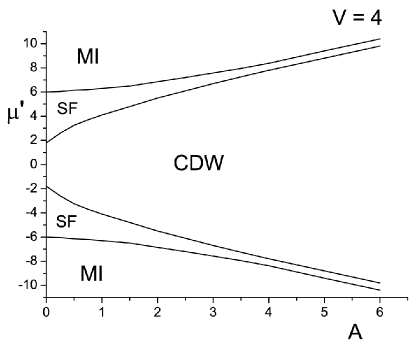
Figure 1: State diagram for a one-dimensional model of ionic conductor at $T=0$; $V=4$, $t=1$ [24].

We performed the numerical calculation of the Drude weight for our model of one-dimensional ionic conductor in different phases based on the formula (4.6). For the Mott insulator (MI) phase (see the phase diagrams [24] and, in particular, the diagram in figure 1) we have got $\langle\hat{T}\rangle=0$ and $\sigma(\omega)=0$ at $T=0$; therefore, $D=0$, exactly as one could expect. At half-filling in CDW phase, the system is also an insulator, so it is expected that in this phase the Drude weight should be also absent (static conductivity must be equal to zero, $D=0$); see for example [8, 42]. However, as follows from our calculations, the Drude weight remains finite ($D>0$) in the case of half-filled CDW phase, but is significantly smaller than in the superfluid (SF) phase. Apparently, this is due to the finite and small size of our one-dimensional cluster ($N=10$). In particular, at $V=4$, $\mu^{\prime}=0$, $A=5$ for CDW phase we have obtained $\frac{1}{N}\langle-\hat{T}\rangle=0.139$, $\int\mathop{\symoperators Re}\nolimits\sigma_{\text{reg}}(\omega)\mathrm{d}\omega=0.043$ and accordingly $D=0.096$. The gap in the CDW phase increases with the modulating field $A$ growth. This leads to the reduction of the calculated Drude weight. We also observe the vanishing of Drude weight for large values of $A$.

For SF phase, if $V=4$, $\mu^{\prime}=-5$ (see figure 1), we obtained $D=0.501$ $(A=0)$, and $D=0.416$ $(A=1)$. The large magnitudes of static conductivity $\sigma(0)$ in SF phase are also found for other values of parameters of the model. More results are shown in tables 1 and 2. Hereinafter, we present the conductivity in relative units omitting the multiplier $\pi q^{2}/\hbar^{2}$ and taking $t=1$. As it follows from the tables, the static conductivity $\sigma(0)$ in SF phase is determined mainly by the mean kinetic energy of ions, while in CDW phase both terms in $D$ should be equal in modulus and compensate each other.

Table 1: Static conductivity (Drude weight) of one-dimensional model of ionic conductor in SF phase ($V=4$, $\mu^{\prime}=-5$, $t=1$) at different values of the modulating field $A$.

$A$	$\frac{1}{N}\langle-\hat{T}\rangle$	$\int\mathop{\symoperators Re}\nolimits\sigma_{\text{reg}}(\omega)\mathrm{d}\omega$	$D$
0	0.501	0.0003	0.501
1	0.424	0.008	0.416

Table 2: Static conductivity (Drude weight) of one-dimensional model of ionic conductor in SF phase ($A=0$, $\mu^{\prime}=-1$, $t=1$) at different values of interaction constant $V$.

$V$	$\frac{1}{N}\langle-\hat{T}\rangle$	$\int\mathop{\symoperators Re}\nolimits\sigma_{\text{reg}}(\omega)\mathrm{d}\omega$	$D$
0	0.524	0	0.524
1	0.607	0.0004	0.607
2	0.588	0.001	0.587

In the absence of interaction between the ions ($V=0$), as well as the modulating field ($A=0$), the current operator commutes with the Hamiltonian and is the integral of motion. Then, $\sigma(\omega\neq 0)=0$ and Drude weight is determined only by the ion kinetic energy. In particular, we have obtained along the lines $V=0$, $A=0$ (see corresponding diagrams [24]): $D=\frac{1}{N}\langle-\hat{T}\rangle=0.524$ at $\mu^{\prime}=-1$, and $D=\frac{1}{N}\langle-\hat{T}\rangle=0.380$ at $\mu^{\prime}=-1.5$. This case corresponds to SF phase.

5 Dynamic part of conductivity

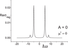
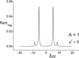
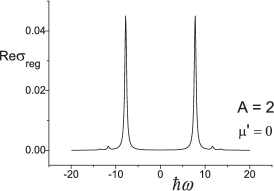
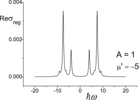
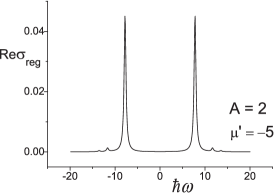
Figure 2: Frequency dependence of the real part of dynamic conductivity of one-dimensional model of the ion conductor at different values of a modulating field $A$ in CDW phase ($\mu^{\prime}=0$), and in SF phase ($\mu^{\prime}=-5$); $N=10$, $V=4$, $t=1$, $\Delta=0.25$.

Table 3: The positions of peaks of dynamic conductivity of one-dimensional model of the ion conductor in CDW phase at different values of the modulating field $A$ and fixed interaction constant $V$: $V=4$ (table on the left) and $V=0$ (table on the right); ($\mu^{\prime}=0$, $t=1$). Let us mention that dashes in certain places in the tables mean a lack of peaks.

$A$	$\hbar\omega_{1}$	$\hbar\omega_{2}$		$A$	$\hbar\omega_{1}$
0	4.92	8.12		0	–
1	5.4	8.6		1	2.36
2	7.8	11.72		2	4.2
3	9.96	–		3	6.12
4	11.96	–		4	8.12
5	14.04	–		5	10.12

Table 4: The positions of peaks of dynamic conductivity of one-dimensional model of the ion conductor in SF phase at different values of the modulating field $A$ and fixed interaction constant $V=4$; ($\mu^{\prime}=-5$, $t=1$).

$A$	$\hbar\omega_{1}$	$\hbar\omega_{2}$
0	5.16	8.36
0.5	3.64	7.0
1	3.96	7.48
1.2	4.2	7.72
2	7.8	11.72

Table 5: The positions of peaks of dynamic conductivity of one-dimensional model of the ion conductor in CDW and SF phases at different values of the interaction constant $V$ and at the absence of a modulating field ($A=0$, $t=1$): CDW phase at $\mu^{\prime}=0$ (the left table) and SF phase at $\mu^{\prime}=-1$ (the right table).

$V$	$\hbar\omega_{1}$	$\hbar\omega_{2}$
0	–	–
1	4.36	6.04
2	4.36	6.68
3	4.52	7.48
4	4.92	8.2
5	5.48	9.0
6	6.2	9.88

$V$	$\hbar\omega_{1}$	$\hbar\omega_{2}$
0	–	–
1	5.0	8.6
2	5.64	11.72
3	4.52	7.48
4	4.92	8.2

 

 

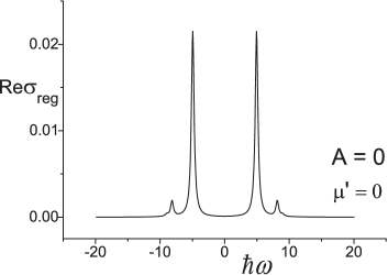
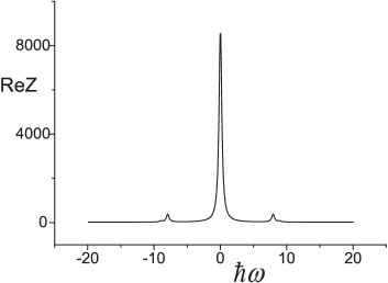
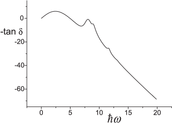
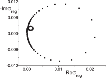
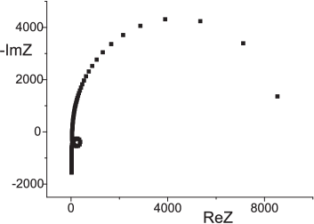
Figure 3: Frequency dependences of the real parts of dynamic conductivity $\mathop{\symoperators Re}\nolimits\sigma_{\text{reg}}$, impedance $\mathop{\symoperators Re}\nolimits Z$ and the loss tangent $\tan\delta$; Nyquist diagrams for CDW phase ($\mu^{\prime}=0$); $N=10$, $V=4$, $A=0$, $t=1$, $\Delta=0.25$.

Dynamic conductivity of one-dimensional ionic chain is calculated according to the formula (3.5). The obtained frequency dependence of the real part of the dynamic conductivity $\mathop{\symoperators Re}\nolimits\sigma_{\text{reg}}(\omega)$ of our one-dimensional model at $T=0$ is presented in figure 2. Here, as an example, the results are shown for the case $V=4$. Two maxima of conductivity (if we consider only positive frequencies $\omega$) are obtained. The diagram in figure 1 shows that the one-dimensional chain at $\mu^{\prime}=0$ is a dielectric in the charge density wave (CDW) state. In the absence of a modulating field ($A=0$), two maxima of conductivity are positioned at frequencies $\hbar\omega_{1}=4.92$, $\hbar\omega_{2}=8.12$. When the modulating field is included, the peak values increase becoming the largest at the field $A\approx 1$. At the further growth of a modulating field, the conductivity monotonously decreases and its two maxima shift to the region of higher frequencies (when $A>2$, one of the peaks practically disappears). In the superfluid phase, the peaks of conductivity are located in the nearly the same frequency region but are slightly displaced. However, their weights are significantly changed. While in CDW phase there is a higher peak at lower frequencies, in the SF phase, on the contrary, the opposite picture is observed. In addition, what is more important, the heights of the peaks are significantly less in the SF phase (up to two orders at $A=0$). When the modulating field is present in SF phase ($\mu^{\prime}=-5$), the heights of the peaks significantly increase, similarly to the case of CDW phase [at $A=2$ we are passing from SF phase to CDW phase (see figure 1) and obtain the conductivity peaks which are characteristic of CDW phase]. Tables 3 and 4 present the frequencies at which the peaks of dynamic conductivity are located: for $V=4$ and $V=0$, depending on the values of the modulating field $A$, and for $A=0$, depending on the values of the interaction $V$ (table 5). As can be seen from the tables, the increase of interaction $V$ constant and the increase of the modulating field $A$ lead to the shift of the peaks of the dynamic conductivity in the direction of higher frequencies. For example, in the case $V=0$ (table 3), we have only one peak of dynamic conductivity in CDW phase; a rough estimate shows the linear dependence of the peak position on the modulating field [$\hbar\omega_{1}(A)\approx 2A$]. In the case of SF phase, the behaviour of the peaks is more complicated (see table 4). Here, the inclusion of a modulating field initially leads to a shift of the peaks towards lower frequencies. At $A=2$ and $V=4$, we come from the SF phase to CDW phase and the peak position coincides with the relevant one for CDW phase (see table 3 and 4). The shift of the peaks affected by interaction $V$ is much weaker. For $A=0$ in CDW phase, it is approximately proportional to $V$ (see table 5). In particular, $\hbar\omega_{1}(V)$ is of the order of $V$, which is in accord with the previous results for conducting phases of 1d models [39] and reflects the similar microscopic nature of the peak appearance.

In figures 3, 4 we presented the calculated frequency dependences of $\mathop{\symoperators Re}\nolimits\sigma$, $\mathop{\symoperators Re}\nolimits Z$ and $\tan\delta$, as well as the Nyquist diagrams for impedance and conductivity in the case of CDW and SF phases. As it follows from the figures, there exists a direct correspondence between the peaks of conductivity and the ellipses or semiellipses in Nyquist plots. In phenomenological description, the existence of two ellipses can be interpreted as manifestation of two types of collective vibrations (‘‘oscillators’’) in the system, which exists due to the interaction between particles. In this connection it is worth mentioning that in the absence of interaction, there is no dynamical part of conductivity in one-dimensional case.

 

 

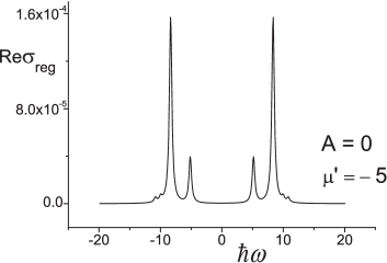
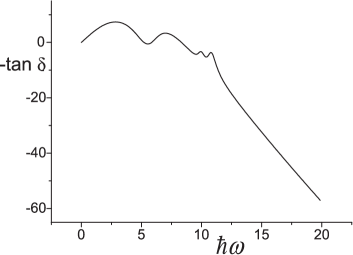
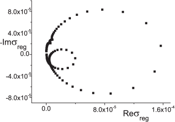
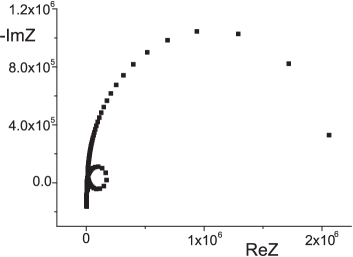
Figure 4: Frequency dependences of the real parts of dynamic conductivity $\mathop{\symoperators Re}\nolimits\sigma_{\text{reg}}$, impedance $\mathop{\symoperators Re}\nolimits Z$ and the loss tangent $\tan\delta$; Nyquist diagrams for SF phase ($\mu^{\prime}=-5$); $N=10$, $V=4$, $A=0$, $t=1$, $\Delta=0.25$.

6 Conclusions

In this paper, using the exact diagonalization method we calculate the energy spectrum and eigenfunctions of the finite one-dimensional model of the ionic conductor with periodic boundary conditions. On the basis of its eigen-states and with the help of Kubo formula we calculate the dynamic conductivity at different values of the interaction constant between particles and the strength of the modulating field. The consideration is performed within the hard-core boson approach (that corresponds to the Pauli statistics). Calculations are made for the case $T=0$.

Based on the results of the energy spectrum calculations [24], we expect that at the transition from CDW-type phase to the superfluid phase, the peaks of dynamic conductivity of the ion chain will shift to the region of lower frequencies. Indeed, in SF phase there are transitions at lower energies than in the CDW phase, but the selection rules for matrices $A^{i}_{pq}$ practically eliminate their contributions to conductivity. Similar results were also obtained by other authors (see for example [7]).

Frequency dependence of dynamic conductivity $\mathop{\symoperators Re}\nolimits\sigma_{\text{reg}}(\omega)$ remains qualitatively unchanged after the transition from CDW phase to SF phase. Only the heights of the maxima of conductivity are changed significantly. In particular, the heights of the peaks are in SF phase of the one order (at $A=1$), or even of the two orders (at $A=0$) less than those in CDW phase. The peaks of the dynamic conductivity in CDW phase shift in the direction of higher frequencies when the values of interaction between the ions $V$ and the modulating field $A$ increase. The effect of the modulating field is here much larger. The peak shift is directly proportional to the field $A$ at $V=0$. As can be seen from the Kubo formula, Drude weight [static conductivity $\mathop{\symoperators Re}\nolimits\sigma(\omega=0)$] is non-zero if there are degenerate states. At $T=0$, this is possible when the ground state is degenerate. We analyzed the energy spectrum obtained in different phases of the finite one-dimensional model of the ion conductor. In all cases, the ground state is nondegenerate (which can be due to finite size of the ion chain), and the Drude weight calculations based on the Kubo formula give the $D=0$ result. Therefore, to calculate the Drude weight we use an alternative way (based on the sum rule) that connects Drude weight with the frequency integrated regular part of conductivity and the average kinetic energy of the ions. In this case, our calculations of $D$ for the half-filled CDW phase still give a non-zero result (which is caused by a finite size of a system), but the obtained value of $D$ is significantly smaller than the one for SF phase [here, the two terms in (4.6) nearly compensate each other]. A significant reduction of the dynamic conductivity in SF phase (compared with CDW phase) leads to a considerable reduction of the second term of Drude weight [$\int\mathop{\symoperators Re}\nolimits\sigma_{\text{reg}}(\omega)\mathrm{d}\omega$] in SF phase and, therefore, the static conductivity in SF phase is mainly determined by the kinetic energy of ions $\frac{1}{N}\langle-\hat{T}\rangle$.

Besides the real part of conductivity, we have also calculated the impedance $Z(\omega)=1/\sigma(\omega)$ and loss tangent $\tan\delta=\mathop{\symoperators Im}\nolimits Z(\omega)/\mathop{\symoperators Re}\nolimits Z(\omega)$. Frequency behaviour of such quantities is important from the point of view of experimental study. In order to interpret the results of the measurements, the Nyquist diagrams (the $\mathop{\symoperators Im}\nolimits Z$ versus $\mathop{\symoperators Re}\nolimits Z$ plots) are usually used. In particular, an important feature of our diagrams is a significant difference in the frequency range of Nyquist plots for CDW and SF phases (up to two orders, as is seen from the presented figures). In practice, it can be used for identifying the state of the ion conducting system.

Ukrainian 0

Динамiчна провiднiсть одновимiрних iонних провiдникiв. Iмпеданс, дiаграми Найквiста

I.В. Стасюк, Р.Я. Стецiв

             
Iнститут фiзики конденсованих систем НАН України, вул. Свєнцiцького, 1, 79011 Львiв, Україна

References

- [1] Mahan G.D., Phys. Rev. B, 1976, 14, 780; doi:10.1103/PhysRevB.14.780.
- [2] Maldague F., Phys. Rev. B, 1977, 16, 2437; doi:10.1103/PhysRevB.16.2437.
- [3] Shastry B.S., Sutherland B., Phys. Rev. Lett., 1990, 65, 243; doi:10.1103/PhysRevLett.65.243.
- [4] Castella H., Zotos X., Prelovšek P., Phys. Rev. Lett., 1995, 74, 972; doi:10.1103/PhysRevLett.74.972.
- [5] Giamarchi T., Phys. Rev. B, 1992, 46, 342; doi:10.1103/PhysRevB.46.342.
- [6] Giamarchi T., Millis A.J., Phys. Rev. B, 1992, 46, 9325; doi:10.1103/PhysRevB.46.9325.
- [7] Kuhner T.D., White S.R., Monien H., Phys. Rev. B, 2000, 61, 12474; doi:10.1103/PhysRevB.61.12474.
-
[8]
Heidrich-Meisner F., Honecker A.,
Cabra D.C., Brenig W., Phys. Rev. B, 2003, 68,
134436;
doi:10.1103/PhysRevB.68.134436. - [9] Mukerjee S., Oganesyan V., Huse D., Phys. Rev. B, 2006, 73, 035113; doi:10.1103/PhysRevB.73.035113.
- [10] Kumar P.P., Yashonath S., J. Chem. Sci., 2006, 118, 135; doi:10.1007/BF02708775.
- [11] Kamaya N., Homma K., Yamakawa Yu., Hirayama M., Kanno R., Yonemura M., Kamiyama T., Kato Yu., Hama S., Kawamoto K., Mitsui A., Nat. Mater., 2011, 10, 682; doi:10.1038/nmat3066.
- [12] Pietraszko A., Goslar J., Hilczer W., Szczepanska L., J. Mol. Struct., 2004, 688, 5; doi:10.1016/j.molstruc.2003.07.013.
-
[13]
Lahajnar G., Blinc R., Dolinsek J.,
Arcon D., Slak J., Solid State Ionics, 1997, 97,
141;
doi:10.1016/S0167-2738(97)00084-2. -
[14]
Yamada M., Mingdeng W., Honma I.,
Haoshen Z., Electrochem. Commun., 2006, 8,
1549;
doi:10.1016/j.elecom.2006.07.020. - [15] Chow E., Delsing P., Haviland D.P., Phys. Rev. Lett., 1998, 81, 204; doi:10.1103/PhysRevLett.81.204.
- [16] Bloch I., Daliberd J., Zwerger W., Rev. Mod. Phys., 2008, 80, 885; doi:10.1103/RevModPhys.80.885.
- [17] Salejda W., Dzhavadov N.A., Phys. Status Solidi B, 1990, 158, 119; doi:10.1002/pssb.2221580111.
- [18] Stasyuk I.V., Pavlenko N., Hilczer B., Phase Transitions, 1997, 62, 135; doi:10.1080/01411599708220065.
- [19] Krasnogolovets V.V., Tomchuk P.M., Phys. Status Solidi B, 1985, 130, 807; doi:10.1002/pssb.2221300247.
- [20] Stasyuk I.V., Vorobyov O., Hilczer B., Solid State Ionics, 2001, 145, 211; doi:10.1016/S0167-2738(01)00960-2.
- [21] Stasyuk I.V., Vorobyov O., Phase Transitions, 2007, 80, 63; doi:10.1080/01411590701315443.
- [22] Stasyuk I.V., Dulepa I.R., Condens. Matter Phys., 2007, 10, 259; doi:10.5488/CMP.10.2.259.
- [23] Stasyuk I.V., Dulepa I.R., J. Phys. Stud., 2009, 13, 2701.
- [24] Stetsiv R.Ya., Stasyuk I.V., Vorobyov O., Ukr. J. Phys., 2014, 59, 515.
- [25] Micnas R., Ranninger J., Robaszkiewicz S., Rev. Mod. Phys., 1990, 62, 113; doi:10.1103/RevModPhys.62.113.
- [26] Micnas R., Robaszkiewicz S., Phys. Rev. B, 1992, 45, 9900; doi:10.1103/PhysRevB.45.9900.
- [27] Rigol M., Muramatsu A., Olshanii M., Phys. Rev. A, 2006, 74, 053616; doi:10.1103/PhysRevA.74.053616.
- [28] Hen I., Rigol M., Phys. Rev. B, 2009, 80, 134508; doi:10.1103/PhysRevB.80.134508.
- [29] Hen I., Iskin M., Rigol M., Phys. Rev. B, 2010, 81, 064503; doi:10.1103/PhysRevB.81.064503.
- [30] Batrouni G.G., Scalettar R.T., Phys. Rev. B, 1992, 46, 9051; doi:10.1103/PhysRevB.46.9051.
- [31] Batrouni G.G., Scalettar R.T., Phys. Rev. Lett., 2000, 84, 1599; doi:10.1103/PhysRevLett.84.1599.
-
[32]
Bernardet K., Batrouni G.G., Meunier J.L.,
Schmid G., Troyer M., Dorneich A., Phys. Rev. B, 2002,
65, 104519;
doi:10.1103/PhysRevB.65.104519. - [33] Bernardet K., Batrouni G.G., Troyer M., Phys. Rev. B, 2002, 66, 054520; doi:10.1103/PhysRevB.66.054520.
- [34] Schmid G., Todo S., Troyer M., Dorneich A., Phys. Rev. Lett., 2002, 88, 167208; doi:10.1103/PhysRevLett.88.167208.
- [35] Guo H.-M., Liang Y., Commun. Theor. Phys. (Beijing, China), 2008, 50, 1142.
- [36] Kampf A.P., Zimanyi G.T., Phys. Rev. B, 1993, 47, 279; doi:10.1103/PhysRevB.47.279.
- [37] Scalapino D.J., White S.R., Zhang S., Phys. Rev. B, 1993, 47, 7995; doi:10.1103/PhysRevB.47.7995.
- [38] Stafford C.A., Millis A.J., Shastry B.S., Phys. Rev. B, 1991, 43, 13660; doi:10.1103/PhysRevB.43.13660.
-
[39]
Fye R.M., Martins M.J., Scalapino D.J.,
Wagner J., Hanke W., Phys. Rev. B, 1991, 44, 6909;
doi:10.1103/PhysRevB.44.6909. - [40] Lindner N.H., Auerbach A., Phys. Rev. B, 2010, 81, 054512; doi:10.1103/PhysRevB.81.054512.
- [41] Kubo R., J. Phys. Soc. Jpn., 1957, 12, 570; doi:10.1143/JPSJ.12.570.
- [42] Scalapino D.J., White S.R., Zhang S.C., Phys. Rev. Lett., 1992, 68, 2830; doi:10.1103/PhysRevLett.68.2830.
Ukrainian \adddialect\l@ukrainian0 \l@ukrainian