Traveling wave solutions to Kawahara and related equations

Abstract

Traveling wave solutions to Kawahara equation (KE), transmission line (TL), and Korteweg-de Vries (KdV) equation are found by using an elliptic function method which is more general than the $\mathrm{tanh}$-method. The method works by assuming that a polynomial ansatz satisfies a Weierstrass equation, and has two advantages: first, it reduces the number of terms in the ansatz by an order of two, and second, it uses Weierstrass functions which satisfy an elliptic equation for the dependent variable instead of the hyperbolic tangent functions which only satisfy the Riccati equation with constant coefficients.

When the polynomial ansatz in the traveling wave variable is of first order, the equation reduces to the KdV equation with only a cubic dispersion term, while for the KE which includes a fifth order dispersion term the polynomial ansatz must necessary be of quadratic type.

By solving the elliptic equation with coefficients that depend on the boundary conditions, velocity of the traveling waves, nonlinear strength, and dispersion coefficients, in the case of KdV equation we find the well-known solitary waves (solitons) for zero boundary conditions, as well as wave-trains of cnoidal waves for nonzero boundary conditions. Both solutions are either compressive (bright) or rarefactive (dark), and either propagate to the left or right with arbitrary velocity.

In the case of KE with nonzero boundary conditions and zero cubic dispersion, we obtain cnoidal wave-trains which represent solutions to the TL equation. For KE with zero boundary conditions and all the dispersion terms present, we obtain again solitary waves, while for KE with all coefficients present and nonzero boundary condition, the solutions are written in terms of Weierstrass elliptic functions. For all cases of the KE we only find bright waves that are propagating to the right with velocity that is a function of both dispersion coefficients.

Keywords: Kawahara equation, KdV equation, transmission line equation, Jacobi and Weierstrass elliptic functions, elliptic function method.

I Introduction

In recent years many methods have been used to find analytic solutions to nonlinear partial differential equations (PDEs). Among the multitude of papers, we shall only refer to two sets of studies which will pertain to this work. The first class of papers are: truncation procedure in the Painlevé analysis Weiss in which authors define the Painlevé property that determines the Lax pairs of the Burgers, KdV, and the modified KdV equations; Hirota bilinear method Hirota where multiple collisions of $N$ solitons with varying amplitudes have been obtained for the KdV equation; the Prelle-Singer method Prelle where a system of differential equations has been shown to have an elementary integral expressible in terms of exponentials, logarithms and algebraic functions; the factorization method Rosu where traveling wave solutions of the standard and compound KdV-Burgers equations are found using factorizations; or the homogeneous balance method Wang where solitary wave solutions of two types of variant Boussinesq equations are obtained. Then, we can also enumerate the trial function method Kud6 where transformations of solutions obtained by the Weiss-Tabor-Carnevale method are used for investigation of Kuramoto-Sivashinsky equation; the nonlinear transformation method Otw where the authors constructed traveling wave solutions for nonlinear diffusion equations with polynomial nonlinearities; the well-known inverse scattering transform Newell ; Ablo and Bäcklund transformation Miura ; the first integral method Nizo where Nizovtseva uses a first integral method which gives singular and kink profiles for the Allen-Cahn hyperbolic equation.

The second class of papers mentioned here are: the simplest equation method Kud5 where Kudrsyashov uses the general solutions of simplest nonlinear differential equations and takes into consideration all possible singularities of Kuramoto- Sivashinsky equation, as well as the equation for description of nonlinear waves in a convective fluid; the $G^{\prime}/G$ expansion method Kud7 where it is shown to be equivalent to the $\tanh$-method first developed by Malfliet and Hereman Malf1 ; Malf2 ; Malf3 ; the automatic method of Parkes Parkes ; the method of $Q$ functions Kud1 ; Kud8 used on Fisher equation and on a seventh order ODE; the generalized Riccati equation method Yan where a new generalized transformation is applied to Whitham-Broer-Kaup (WBK) equation; the $\sinh$-$\cosh$-method Was where the author finds solitons, kinks, and periodic solutions of Benjamin-Bona-Mahony (BBM) equation; the modified $\tanh$-method Fan1 ; Fan2 where the author uses a modified by a parameter Riccati equation; the algebraic method where algorithms using sophisticated Mathematica programs are used to find closed-form solutions in terms of Jacobi elliptic functions Bald ; Her ; the $\mathrm{sech}$-method Ma to find solitons to a seventh order KdV equation. Then we also include the Jacobi elliptic function method Fan3 used on a double sine-Gordon, Hirota equation, and the coupled Schrödinger-KdV system; the work of Fu and Liu Fu ; Liu on Jacobi elliptic function expansion method; and Porubov Por1 ; Por2 ; Por3 on traveling periodic solutions of a pair of coupled nonlinear Schrödinger equations obtained in terms of Weierstrass elliptic $\wp$ functions.

More importantly, if for the former class of papers the methods yield restrictive solutions involving elementary functions which generate solitary waves, singular solutions as rational functions, periodic trigonometric solutions, kinks and fronts, the latter studies involve finding analytical solutions of evolution equations in terms of Jacobi, Weierstrass or elliptic theta functions.

Motivated by the work of the authors of the second class of papers, an elliptic function method, which is easier to implement and more general than the hyperbolic tangent method is applied to a nonlinear dispersive PDE known as Kawahara equation (KE) to find periodic solutions in terms of Weierstrass $\wp$ elliptic functions, Jacobi elliptic or hyperbolic functions. This equation takes the form

$$u_{t}+\kappa uu_{x}+\alpha u_{xxx}-\beta u_{xxxxx}=0,$$ (1)

and was investigated numerically in a study of magneto-acoustic waves in a cold collision-free plasma Kawa5 . The coefficients of this equations are: $\alpha,\beta$ - third and fifth order dispersive terms, $\kappa$ - the strength of the nonlinearity (wave steepening) and are real constants. We may assume that $\beta>0$, because by the transformations $u\rightarrow-u,$ $x\rightarrow-x,$ and $t\rightarrow-t,$ we obtain the same equation as (1) with the dispersive terms reversed in sign Kawa5 . Under certain circumstances, the third order dispersion coefficient $\alpha$ becomes very small, or even zero, so one should include the higher order dispersion $\beta$ which will balance the nonlinear effect $\kappa$ Kuka ; Has .

We can write Eq. (1) in Hamiltonian form Drazin

$$u_{t}=\frac{\partial}{\partial x}\left(\frac{\delta\mathcal{H}}{\delta u}\right),$$ (2)

where the Hamiltonian is

$$\mathcal{H}=-\frac{1}{6}\kappa u^{3}+\frac{1}{2}\alpha{u_{x}}^{2}+\frac{1}{2}\beta{u_{xx}}^{2}.$$ (3)

Using this Hamiltonian, KE (1) has the conserved energy density

$$\mathcal{I}=\int_{-\infty}^{\infty}\mathcal{H}dx.$$ (4)

By using the Fréchet derivative which corresponds to the Euler-Lagrange operator

$$\frac{\delta}{\delta u}=\frac{\partial}{\partial u}-\frac{d}{dx}\frac{\partial}{\partial u_{x}}+\frac{d^{2}}{dx^{2}}\frac{\partial}{\partial u_{xx}},$$ (5)

then Eq. (2) becomes KE (1).

By applying a traveling wave ansatz $u(\xi)=u(x-ct)$, with $c$ being the velocity of the unidirectional traveling wave in the $x$ direction at time $t$, yields a fifth order ordinary differential equation (ODE) in the traveling wave variable $\xi$

$$-cu_{\xi}+\kappa uu_{\xi}+\alpha u_{\xi\xi\xi}-\beta u_{\xi\xi\xi\xi\xi}=0.$$ (6)

By one integration this reduces to the fourth order ODE

$$-cu+\frac{\kappa}{2}u^{2}+\alpha u_{\xi\xi}-\beta u_{\xi\xi\xi\xi}=\mathcal{A}$$ (7)

with $\mathcal{A}$ an arbitrary integration constant which can be zero or not depending on the types of boundary conditions chosen. By multiplying by $u_{\xi}$ and integrating once we obtain a conserved quantity for Eq. (1) in the traveling wave variable $\xi$

$$\mathcal{C}=-2\mathcal{A}u-cu^{2}+\frac{\kappa}{3}u^{3}+\alpha{u_{\xi}}^{2}-\beta\left[2u_{\xi}u_{\xi\xi\xi}-(u_{\xi\xi})^{2}\right]\equiv const.$$ (8)

In his comment to Assas’ paper Assa10 , Kudryashov developed the solutions of KE using the tanh-method Kud3 ; Kud2 . This method was originally used by Malfliet and Hereman Malf1 ; Malf2 ; Malf3 and has the advantage of reducing nonlinear ODEs into systems of algebraic equations, that might be easier to solve. Kudryashov explained that Eq. (7) does not pass the Painlevé test, but nevertheless one can find solitary waves of higher order by writing the Laurent series expansion for a function $Y(\xi)$ which must include a pole of order four Kud1 ; Kud4 , where the function in the expansion solves the Riccati equation with constant coefficients

$$Y_{\xi}=\eta(1-Y^{2})$$ (9)

with solution $Y(\xi)=\mathrm{tanh}(\eta\xi)$. Therefore, if we assume solutions of the form

$$u(\xi)=\sum_{i=0}^{n}C_{i}Y^{i},$$ (10)

once the numbers of terms $n$ is determined using the balancing principle Nick , we can write the solutions of Eq. (7) in terms of the solutions of the Riccati equation (9). Since the hyperbolic tangent solution is a particular solution of the Riccati equation, and any other solution can be found using the transformation $Y=\mathrm{tanh}(\eta\xi)+\frac{1}{W}$, where $W$ satisfies a first order linear equation, then all the other solutions which are meromorphic to $u$ can be written using a new expansion in $W$ with the same number of terms. More than that, all forms of the general solution of the Riccati equation have the same Laurent series and they differ only by arbitrary constants Ere . Therefore, using different ODEs as generators of particular solutions, one can find a rich class of meromorphic solutions to evolution equations, which unite many approaches involving elementary functions. These methods are not restrictive to only parabolic equations ($d/dt\rightarrow-c~{}d/d\xi$), as they were also successfully implemented to find solutions to hyperbolic PDEs ($d^{2}/dt^{2}\rightarrow c^{2}~{}d^{2}/d{\xi}^{2}$) such as Boussinesq Wang and improved Boussinesq equation Kud2 ; Ablo , Klein-Gordon Zhang , and Allen-Cahn equation via the first integral method Nizo . Note that the elliptic function method will not work if the ODE contains both even and odd derivative terms, see Lemma V.1. in the Appendix, for the explanation.

In order to determine the number of terms in the expansion of the ansatz, we compute the second order derivative $d^{2}/d\xi^{2}$ for which the leading term is $\eta^{2}(1-Y^{2})^{2}~{}d^{2}/dY^{2}$, while for the fourth order derivative $d^{4}/d\xi^{4}$ the leading term is $\eta^{4}(1-Y^{2})^{4}~{}d^{4}/dY^{4}$. Thus, when we balance the nonlinear term with the higher order derivatives, we must distinguish between two different cases. When $\beta=0$ (KdV equation), we only need to balance $u_{\xi\xi}$ with $u^{2}$ which leads to $4+(n-2)=2n\Rightarrow n=2$. For the second case (KE), we balance $u_{\xi\xi\xi\xi}$ with $u^{2}$ which leads to $8+(n-4)=2n\Rightarrow n=4$. Therefore, the solutions for the KdV or KE must take the form

$$u(\xi) =A_{0}+A_{2}~{}\mathrm{tanh}^{2}(\eta\xi),\quad\quad\beta=0$$ (11)

$$u(\xi) =B_{0}+B_{2}~{}\mathrm{tanh}^{2}(\eta\xi)+B_{4}~{}\mathrm{tanh}^{4}(\eta\xi),\quad\quad\beta\neq 0$$

with the first and third order coefficients identically zero Kud2 .

Since KdV equation also possesses non elementary solutions in terms of Jacobi elliptic functions KdV which are not solutions of the Riccati equation (9), we extend the ansatz of the function $Y$ and we replace the Riccati equation by an elliptic equation, i.e., the function $Y$ in the new ansatz given by (10) satisfies

$${Y_{\xi}}^{2}=a_{0}+a_{1}Y+a_{2}Y^{2}+a_{3}Y^{3},\quad\quad a_{3}\neq 0.$$ (12)

This new ansatz has the advantage of extending the classes of solutions to include elliptic functions Fan3 ; Liu ; Kud5 , and as a special case when two of the roots of the cubic polynomial in $Y$ collide, the solitary waves can be recovered as a limit case of cnoidal waves Man2 ; Man3 . The constants $a_{i}$ which depend on the system parameters $\alpha,\beta,\kappa$, the speed $c$, and boundary conditions $\mathcal{A}$ respectively, can be found algebraically after the ansatz passes the balancing principle Nick , which will determine the number of terms $n$ in the expansion given by (10).

Using the new ansatz, and by balancing, we obtain $n+1=2n\Rightarrow n=1$ when $\beta=0$ and $n+2=2n\Rightarrow n=2$ when $\beta\neq 0$. Therefore, by replacing Riccati equation (9) with the elliptic equation (12), we reduce the numbers of terms in half in the expansion of Eq. (10) which is now only linear for KdV or quadratic for KE

$$u(\xi) =A_{0}+A_{1}Y,\quad\quad\beta=0$$ (13)

$$u(\xi) =B_{0}+B_{1}Y+B_{2}Y^{2},\quad\quad\beta\neq 0.$$

II Reduction to the KdV equation ($\beta=0$)

When $\beta=0$, Eq. (1) reduces to the KdV equation which describes the motion of small amplitude and large wavelength shallow waves in dispersive systems KdV

$$u_{t}+\kappa uu_{x}+\alpha u_{xxx}=0.$$ (14)

By using $\beta=0$ in Eq. (7), we obtain the second order ODE in $u$

$$-cu+\frac{\kappa}{2}u^{2}+\alpha u_{\xi\xi}=\mathcal{A}.$$ (15)

Without loss of generality we may assume that $A_{0}=0$, $A_{1}=1$ so that $u=Y$. To find the solutions of Eq. (15) using our procedure, we differentiate Eq. (12) to obtain higher derivatives of $Y$

$$Y_{\xi\xi} =\frac{1}{2}a_{1}+a_{2}Y+\frac{3}{2}a_{3}Y^{2}$$ (16)

$$Y_{\xi\xi\xi} =(a_{2}+3a_{3}Y)Y_{\xi}$$

$$Y_{\xi\xi\xi\xi} =3a_{0}a_{3}+\frac{1}{2}a_{1}a_{2}+\left(\frac{9}{2}a_{1}a_{3}+{a_{2}}^{2}\right)Y+\frac{15}{2}a_{2}a_{3}Y^{2}+\frac{15}{2}{a_{3}}^{2}Y^{3},$$

and by substituting them into Eq. (1) we obtain a cubic polynomial in $Y$

$$\sum_{i=0}^{3}s_{i}Y^{i}\equiv 0,$$ (17)

with coefficients $s_{i}$ given by the expressions

$$\begin{array}[]{l}s_{3}=-\frac{15}{2}{a_{3}}^{2}\beta\\ s_{2}=\frac{1}{2}\left[\kappa+3a_{3}(\alpha-5a_{2}\beta)\right]\\ s_{1}=-c+a_{2}\alpha-{a_{2}}^{2}\beta-\frac{9}{2}a_{1}a_{3}\beta\\ s_{0}=-\mathcal{A}-3a_{0}a_{3}\beta+\frac{a_{1}}{2}(\alpha-a_{2}\beta).\end{array}$$ (18)

Because all these coefficients must be zero, and since $a_{3}\neq 0$, from the first equation of the system (18), we immediately conclude that $\beta=0$, so the reduced constants become

$$\begin{array}[]{l}s_{2}=\frac{1}{2}\left(\kappa+3a_{3}\alpha\right)\\ s_{1}=-c+a_{2}\alpha\\ s_{0}=-\mathcal{A}+\frac{a_{1}}{2}\alpha.\end{array}$$ (19)

By solving simultaneously $s_{i}=0$ for the coefficients $a_{i}$, Eq. (12) becomes

$${Y_{\xi}}^{2}=a_{0}+\frac{2\mathcal{A}}{\alpha}Y+\frac{c}{\alpha}Y^{2}-\frac{\kappa}{3\alpha}Y^{3}\equiv q_{3}(Y),$$ (20)

where $a_{0}$ is an arbitrary constant. According to Eq. (8) the conserved quantity in $\xi$ for the KdV equation is

$$\mathcal{C}=-2\mathcal{A}Y-cY^{2}+\frac{\kappa}{3}Y^{3}+\alpha{Y_{\xi}}^{2},$$ (21)

and by comparing Eqs. (20) and (21) we identify $a_{0}=\frac{\mathcal{C}}{\alpha}$, so the arbitrary constant of the elliptic equation is proportional to the conserved quantity, and inverse proportional to the cubic dispersion. The elliptic solutions of Eq. (20) depend on the type of roots of the cubic polynomial $q_{3}(Y)$, which automatically leads to the following sub-cases:

i) One zero root of multiplicity two, and one simple root $Y_{0}=\frac{3c}{\kappa}$. This is achieved when we choose zero boundary conditions $\mathcal{A}=0$ together with $a_{0}=0$, i.e., the fluid is undisturbed at infinity ($Y,Y_{\xi},Y_{\xi\xi}\rightarrow 0$ as $|\xi|\rightarrow\infty$). By letting $\frac{\kappa}{3\alpha}=\frac{1}{\sigma}$ we factor Eq. (20) as

$${Y_{\xi}}^{2}=\frac{1}{\sigma}Y^{2}(Y_{0}-Y),$$ (22)

with solution the solitary wave KdV ; Rey

$$Y(\xi)=Y_{0}\mathrm{sech}^{2}\left[\frac{1}{2}\sqrt{\frac{Y_{0}}{\sigma}}(\xi-\xi_{0})\right]$$ (23)

which propagates with velocity proportional to amplitude $Y_{0}$, and width inverse proportional to the square root of $Y_{0}$.

Now we must discuss the sign of $\sigma$. First possibility is that $\sigma>0$ so $\kappa$ and $\alpha$ are of the same sign, and because $Y_{\xi}\in{\mathbb{R}}$ we must have $Y_{0}>0$ which means that $c$ is the same sign as $\alpha$ and $\kappa$. These waves travel to the right ($c>0$) in a positive strength ($\kappa>0$) and positive dispersive medium ($\alpha>0$), and to the left ($c<0$) in a negative strength ($\kappa>0$) negative dispersive medium ($\alpha<0$). In both cases their amplitude is always positive and they represent the positive (compressive/ bright) solitary waves. On the other hand, if $\sigma<0$ so that $\kappa$ and $\alpha$ are of opposite signs, then we must have $Y_{0}<0$. Therefore, these are waves that travel to the right ($c>0$) in a negative strength ($\kappa<0$) and positive dispersive medium ($\alpha>0$) medium, and to the left ($c<0$) in a positive strength ($\kappa>0$) and negative dispersive medium ($\alpha<0$). In both cases their amplitude is always negative and they represent the negative (rarefactive/ dark) solitary waves KdV ; Rey . For all other remaining combination of coefficients, the solitons become unbounded and solutions are unphysical, when the hyperbolic secant becomes periodic with poles aligned on the real $\xi$-axis. For the solitonic case, and regardless of the signs of the coefficients, for $\xi_{0}=0$ and $u=Y$ the solution is

$$u(x,t)=\frac{3c}{\kappa}\mathrm{sech}^{2}\left[\frac{1}{2}\sqrt{\frac{c}{\alpha}}(x-ct)\right]$$ (24)

If the velocity is fixed, the amplitude and width can be manipulated using the strength and dispersion coefficients. When $\kappa$ is big the amplitude is small, and when $\alpha$ is small the solitons are thin, while increasing the dispersion it increases their widths when solitons spread, see Fig. 1 for the values of $\alpha=1$, $\kappa=1$ and $\alpha=-5$, $\kappa=-5$ for bright solitons (top panel), and $\alpha=1$, $\kappa=-5$ and $\alpha=-5$, $\kappa=1$ for dark solitons (bottom panel).

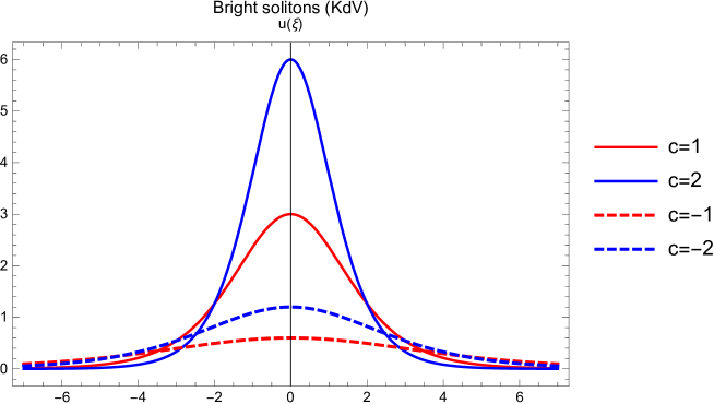
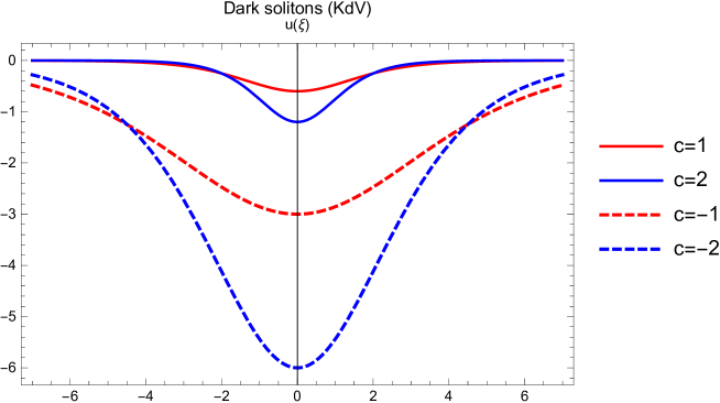
Figure 1: Bright solitons for the KdV Eq. (14) with zero boundary conditions $\mathcal{A}=0$ and $\alpha=1,~{}\kappa=1$ (continuous curves) when solitons propagate to the right, and $\alpha=-5,~{}\kappa=-5$ (dashed curves) when solitons propagate to the left (top panel). Dark solitons for the KdV Eq. (14) with zero boundary conditions $\mathcal{A}=0$ and $\alpha=1,~{}\kappa=-5$ (continuous curves) when solitons propagate to the right, and $\alpha=-5,~{}\kappa=1$ (dashed curves) when solitons propagate to the left (bottom panel).

ii) Now we drop the assumption that fluid must be undisturbed at infinity, so then we must have $Y_{\xi}=0$ for $Y=0$ which implies that only one root is zero. This corresponds to setting $a_{0}=0$, while the other two roots are real and distinct. Under these assumptions Eq.(20) can be factored as

$${Y_{\xi}}^{2}=\frac{1}{\sigma}~{}Y(Y_{2}-Y)(Y_{3}+Y),$$ (25)

where $Y_{2,3}$ satisfy

$$\begin{array}[]{l}Y_{2}=\frac{Y_{0}\pm\sqrt{\Omega}}{2}\\ Y_{3}=\frac{-Y_{0}\pm\sqrt{\Omega}}{2}.\end{array}$$ (26)

For real roots we require the discriminant $\Omega=\frac{9c^{2}+24\mathcal{A}\kappa}{\kappa^{2}}>0$, which restricts the values for $\mathcal{A}$ and $\kappa$ such that $\mathcal{A}\kappa>-\frac{3c^{2}}{8}$. The solution of Eq. (25) is

$$u(\xi)=Y_{2}~{}\mathrm{cn}^{2}\left[\frac{1}{2}\sqrt{\frac{1}{\sigma}(Y_{2}+Y_{3})}(\xi-\xi_{0});m\right],$$ (27)

which simplifies to

$$u(\xi)=\frac{Y_{0}\pm\sqrt{\Omega}}{2}\mathrm{cn}^{2}\left[\frac{1}{2}\sqrt{\pm\frac{\sqrt{\Omega}}{\sigma}}(\xi-\xi_{0});\sqrt{\frac{1}{2}\pm\frac{Y_{0}}{2\sqrt{\Omega}}}\right],$$ (28)

where $\mathrm{cn}(\theta;m)$ is the Jacobian elliptic function with modulus $m=\sqrt{\frac{Y_{2}}{Y_{2}+Y_{3}}}$. Using the values of the roots from system (26), and $\xi_{0}=0$ the solutions of the KdV equation (14) with nonzero boundary conditions are

$$u(x,t)=\begin{array}[]{lr}\frac{3c\pm\sqrt{9c^{2}+24\mathcal{A}\kappa}}{2\kappa}\mathrm{cn}^{2}\left[\frac{1}{2}\frac{\sqrt[4]{9c^{2}+24\mathcal{A}\kappa}}{\sqrt{\pm 3\alpha}}(x-ct);\sqrt{\frac{1}{2}\pm\frac{3c}{2\sqrt{9c^{2}+24\mathcal{A}\kappa}}}\right].\end{array}$$ (29)

If $\alpha,\kappa$ have same sign then $\sigma>0$, so $Y_{2}+Y_{3}=\sqrt{\Omega}>0$, and we obtain bright cnoidal waves which propagate to the right ($c>0$) or to the left ($c<0$), see Fig. 2 (top panel) for right waves with $\alpha=1$, $\kappa=2$, and left waves with $\alpha=-2$, $\kappa=-2$. Otherwise, when $\alpha,\kappa$ have opposite sign then $\sigma<0$, so $Y_{2}+Y_{3}=-\sqrt{\Omega}<0$, and we obtain dark cnoidal waves which also propagate to the right ($c>0$) or to the left ($c<0$), see Fig. 2 (bottom panel) for right waves with $\alpha=-1$, $\kappa=2$, and left waves with $\alpha=2$, $\kappa=-1$. These solutions represent trains of periodic cnoidal waves with shape and wavelength that depend on the amplitude of the waves. The wavelength is $\lambda=4\sqrt{\frac{\pm\sigma}{\sqrt{\Omega}}}K(m)$, where $K(m)$ is the complete elliptic integral of first kind given by $K(m)=\int_{0}^{\frac{\pi}{2}}\frac{d\theta}{\sqrt{1-m^{2}\sin^{2}\theta}}$.

Figure 2: Bright cnoidal waves for the KdV Eq. (14) with $\alpha=1,~{}\kappa=2,~{}\mathcal{A}=1$ (continuous curves) when the waves propagate to the right, and $\alpha=-2,~{}\kappa=-2~{}\mathcal{A}=-1$ (dashed curves) when the waves propagate to the left (top panel). Dark cnoidal waves for the KdV Eq. (14) with $\alpha=-1,~{}\kappa=2,~{}\mathcal{A}=1$ (continuous curves) when the waves propagate to the right, and $\alpha=2,~{}\kappa=-1,~{}\mathcal{A}=-1$ (dashed curves) when the waves propagate to the left (bottom panel).

When $\mathcal{A}\rightarrow 0$, and depending on the modulus $m$ we have two extreme cases. First, by choosing the negative branch of the sqare root $Y_{2}\rightarrow 0\Rightarrow m\rightarrow 0$, and $\mathrm{cn~{}\theta}\rightarrow\cos\theta$, thus cnoidal waves resemble more sinusoidal waves of unchanging shape discovered by Stokes, which in the theory of long waves constitutes a particular case of cnoidal form Sto ; KdV . Second, by choosing the positive branch of the square root $Y_{3}\rightarrow 0\Rightarrow m\rightarrow 1$, and $\mathrm{cn~{}\theta}\rightarrow\mathrm{sech}~{}\theta$, thus cnoidal waves loose their periodicity, and reduce to the solitary waves given by Eq. (24).

III Kawahara equation ($\beta\neq 0$)

By using the second equation of system (13) with $B_{0}=0$, $B_{1}=0$, $B_{2}=1$ and $u=Y^{2}$, the derivatives of $u$ become

$$\begin{array}[]{l}u_{\xi\xi}=2({Y_{\xi}}^{2}+YY_{\xi\xi})\\ u_{\xi\xi\xi}=2(3Y_{\xi}Y_{\xi\xi}+YY_{\xi\xi\xi})\\ u_{\xi\xi\xi\xi}=2[3(Y_{\xi\xi})^{2}+4Y_{\xi}Y_{\xi\xi\xi}+YY_{\xi\xi\xi\xi}].\end{array}$$ (30)

Using the derivatives of $Y$ from system (16) in system (30), the second and fourth order derivatives of $u$ as function of $Y$ become

$$u_{\xi\xi} =2a_{0}+3a_{1}Y+4a_{2}Y^{2}+5a_{3}Y^{3}$$ (31)

$$u_{\xi\xi\xi\xi} =\frac{3}{2}{a_{1}}^{2}+8a_{0}a_{2}+15(a_{1}a_{2}+2a_{0}a_{3})Y+2(8{a_{2}}^{2}+21a_{1}a_{3})Y^{2}$$

$$+65a_{2}a_{3}Y^{3}+\frac{105}{2}{a_{3}}^{2}Y^{4}.$$

By substituting these derivatives in Eq. (7) we obtain the quartic polynomial in $Y$

$$\sum_{i=0}^{4}r_{i}Y^{i}\equiv 0,$$ (32)

with coefficients given by

$$\begin{array}[]{l}r_{4}=\frac{1}{2}(\kappa-105{a_{3}}^{2}\beta)\\ r_{3}=5a_{3}(\alpha-13a_{2}\beta)\\ r_{2}=-c+4a_{2}\alpha-16{a_{2}}^{2}\beta-42a_{1}a_{3}\beta\\ r_{1}=-30a_{0}a_{3}\beta+3a_{1}(\alpha-5a_{2}\beta)\\ r_{0}=-\mathcal{A}-\frac{3}{2}{a_{1}}^{2}\beta+2a_{0}(\alpha-4a_{2}\beta).\end{array}$$ (33)

Since all coefficients $r_{i}=0$, by simultaneously solving the first four equations of system (33) we find

$$\begin{array}[]{l}a_{3}=\mp\sqrt{\frac{\kappa}{105\beta}}\\ a_{2}=\frac{\alpha}{13\beta}\\ a_{1}=\sqrt{\frac{5}{21\kappa\beta}}\frac{\mp 36\alpha^{2}\pm 169c\beta}{2\cdot 169\beta}\\ a_{0}=\frac{2\alpha(36\alpha^{2}-169c\beta)}{13^{3}\kappa\beta^{2}}.\end{array}$$ (34)

For real coefficients, and since $\beta>0$, we require that the wave steepening coefficient $\kappa>0$. By using these coefficients together with the last equation of system (33), we find the integration constant to be

$$\mathcal{A}=\frac{(36\alpha^{2}-169\beta c)(2^{2}\cdot 3^{3}\cdot 17~{}\alpha^{2}+5\cdot 169\beta c)}{2^{3}\cdot 7\cdot 13^{4}\kappa\beta^{2}}.$$ (35)

This shows that while for KdV equation the boundary $\mathcal{A}$ is arbitrary, for KE the boundary $\mathcal{A}$ is fixed by the system’s parameters $\alpha,\beta,\kappa$ and the speed $c$. This means that traveling waves for KE can change shape depending if the speed $c$ is chosen such a way that $\mathcal{A}$ is zero or not.

III.1 Transmission line equation

Now we analyze the special case of $\alpha=0$ which from system (34) leads to $a_{2}=a_{0}=0$ so that Eq. (1) includes a fifth order dispersion term only, and takes the form

$$u_{t}+\kappa uu_{x}-\beta u_{xxxxx}=0.$$ (36)

This equation describes pulses over a transmission line containing a large number of LC circuits, and it occurs by making use of mutual inductance between neighboring inductors. It was first studied by Hasimoto Has for shallow water waves near some critical value of surface tension, while Nagashima Naga1 performed experiments, and observed the solitary waves using an oscilloscope. Later, in a more general setting, it was also derived by Rosenau using a quasi-continuous formalism that included higher order discrete effects Ros1 ; Ros2 .

For $\alpha=0$ Eq. (7) becomes

$$-cu+\frac{\kappa}{2}u^{2}-\beta u_{\xi\xi\xi\xi}=\mathcal{A},$$ (37)

so Eq. (12) corresponds to

$${Y_{\xi}}^{2}=Y(a_{1}+a_{3}Y^{2}),$$ (38)

which is in fact a special case of Eq. (25) for a real root that has multiplicity two, $Y_{2}=Y_{3}$. The reduced coefficients obtained from system (34) are given by the expressions

$$\begin{array}[]{l}a_{3}=\mp\sqrt{\frac{\kappa}{105\beta}}\\ a_{1}=\pm\frac{c}{2}\sqrt{\frac{5}{21\kappa\beta}},\end{array}$$ (39)

and are used to factor Eq. (38) to obtain

$${Y_{\xi}}^{2}=-a_{3}Y({Y_{2}}^{2}-Y^{2}),$$ (40)

with ${Y_{2}}^{2}=-\frac{a_{1}}{a_{3}}=\frac{5c}{2\kappa}$. Since $a_{1},a_{3}$ have opposite signs, then ${Y_{2}}^{2}>0$, and because $a_{1},a_{3}\in{\mathbb{R}}\Rightarrow\kappa>0$, thus as before, the waves propagate only to the right ($c>0$). By integrating Eq. (40), and using formula (27) we obtain the special cnoidal wave of constant modulus

$$Y(\xi)=Y_{2}~{}\mathrm{cn}^{2}\left[\frac{\sqrt{2}}{2}\sqrt{-a_{3}Y_{2}}(\xi-\xi_{0});\frac{\sqrt{2}}{2}\right].$$ (41)

The wavelength of the waves is $\lambda=2\sqrt{2}K\left(\frac{\sqrt{2}}{2}\right)\sqrt[4]{\frac{42\beta}{c}}$, where $K\left(\frac{\sqrt{2}}{2}\right)=1.85407$, so the periodicity is only a function of the speed $c$ and dispersion $\beta$. Using the values of $Y_{2}$, $a_{3}$, $u=Y^{2}$ and $\xi_{0}=0$ the solution to the transmission line equation (36) with nonzero boundary condition is

$$u(x,t)=\frac{5c}{2\kappa}~{}\mathrm{cn}^{4}\left[\frac{\sqrt{2}}{2}\sqrt[4]{\frac{c}{42\beta}}~{}(x-ct);\frac{\sqrt{2}}{2}\right].$$ (42)

This solution was also obtained by Yamamoto Yama7 , Kano Kano4 and Kudryashov Kud2 , and represents a train of periodic waves with fixed modulus which tells that the shape is preserved as the pulse travels over the transmission line, see Fig. 3 for the values of $\beta=1,\kappa=2$.

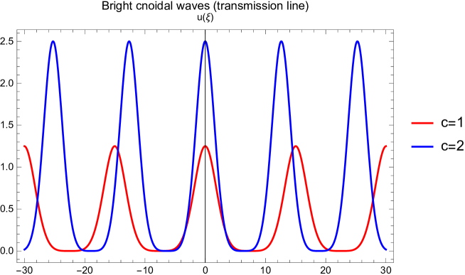
Figure 3: Bright cnoidal waves for the transmission line equation (36) with nonzero boundary conditions for $\alpha=0,\beta=1,\kappa=2$.

III.2 KE with zero boundary conditions

Traveling waves with zero boundary condition $\mathcal{A}=0$ yield waves which propagate with velocities $c=-\frac{2^{2}\cdot 3^{3}\cdot 17\alpha^{2}}{5\cdot 169\beta}<0$ or $c=\frac{36\alpha^{2}}{169\beta}>0$.

i) For left traveling waves, the modular discriminant obtained from the last equation of system (54) becomes $\Delta=-\frac{6\cdot 1523\alpha^{6}}{5^{4}\cdot 13^{6}\beta^{6}}<0$, so the polynomial $s_{3}(t)$ given by Eq. (53) has non real roots, and because is an unphysical case it will be omitted.

ii) For right traveling waves, the system (34) reduces to

$$\begin{array}[]{l}a_{3}=\mp\sqrt{\frac{\kappa}{105\beta}}\\ a_{2}=\frac{\alpha}{13\beta}\\ a_{1}=a_{0}=0\\ \end{array}$$ (43)

with corresponding elliptic equation

$${Y_{\xi}}^{2}=a_{3}Y^{2}\left(Y+\frac{a_{2}}{a_{3}}\right),$$ (44)

Letting $Y\rightarrow-\tilde{Y}$, and using solution (23) we obtain

$$Y(\xi)=-\tilde{Y}(\xi)=-\frac{a_{2}}{a_{3}}\mathrm{sech}^{2}\left[\frac{1}{2}\sqrt{a_{2}}(\xi-\xi_{0})\right].$$ (45)

Therefore, right traveling wave solution of the KE with zero boundary condition and $\xi_{0}=0$ reduces to

$$u(x,t)=\frac{105\alpha^{2}}{169\kappa\beta}\mathrm{sech}^{4}\left[\frac{1}{2}\sqrt{\frac{\alpha}{13\beta}}\left(x-\frac{36\alpha^{2}}{169\beta}t\right)\right].$$ (46)

Since $\beta>0\Rightarrow\alpha>0$, and since $a_{3}\in{\mathbb{R}}\Rightarrow\kappa>0$, and we obtain bright solitons which only propagate to the right. Let us rescale the solution according to the new variables

$$\gamma=4\sqrt{\frac{\kappa}{105\beta}},\delta=\frac{4\alpha}{13\beta}\Rightarrow c=\frac{9\beta}{4}\delta^{2},$$ (47)

so the solitons take the simpler form

$$u(x,t)=\left(\frac{\delta}{\gamma}\right)^{2}\mathrm{sech}^{4}\left[\frac{1}{4}\sqrt{\delta}\left(x-\frac{9}{4}\delta^{2}t\right)\right].$$ (48)

This solution written in the same manner was also derived by Yamamoto Yama7 , Yuan Yuan0 and Rosenau Ros2 using different approaches, and shows once again that the speed of the wave is proportional to the height and inverse proportional to the width, as it is the case of the KdV equation, with the difference that while for the KdV the solitons propagate with arbitrary velocity, for KE they translate with velocity that is fixed by both dispersion coefficients. In Fig. 4 we plot the solitary waves that propagate to the right for the values of $\alpha=2,\kappa=5$ for which $\gamma=\frac{4}{\sqrt{21\beta}}$ and $\delta=\frac{8}{13\beta}$. Fixing the velocities $c=1,2$ we obtain the values for the dispersion coefficient to be $\beta=\frac{144}{169},\frac{72}{169}$.

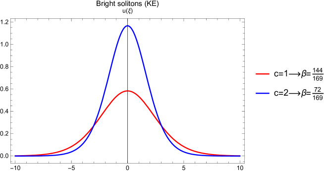
Figure 4: Bright solitons for the KE (1) with zero boundary conditions $\mathcal{A}=0$ and $\alpha=2,\kappa=5$. When $c=1,2$ then $\beta=\frac{144}{169},\frac{72}{169}.$

III.3 KE with nonzero boundary conditions

When all the coefficients from system (34) are nonzero, we solve Eq. (12) by reduction to the Weierstrass elliptic equation Manc

$$\wp_{\xi}^{2}=4\wp^{3}-g_{2}\wp-g_{3},$$ (49)

by the scale-shift linear transformation

$$Y(\xi)=\frac{4}{a_{3}}\wp(\xi-\xi_{0};g_{2},g_{3})-\frac{a_{2}}{3a_{3}}.$$ (50)

The invariants of the Weierstrass function are given by

$$\begin{array}[]{l}g_{2}=\frac{{a_{2}}^{2}-3a_{1}a_{3}}{12}=2({e_{1}}^{2}+{e_{2}}^{2}+{e_{3}}^{2})\\ g_{3}=\frac{3^{2}a_{1}a_{2}a_{3}-3^{3}a_{0}{a_{3}}^{2}-2{a_{2}}^{3}}{16\cdot 3^{3}}=4e_{1}e_{2}e_{3},\end{array}$$ (51)

and together with the modular discriminant

$$\Delta={g_{2}}^{3}-3^{3}{g_{3}}^{2}=16(e_{1}-e_{2})^{2}(e_{1}-e_{3})^{2}(e_{2}-e_{3})^{2}$$ (52)

are used to classify the solutions of Eq. (12). The constants $e_{i}$ are the roots of the cubic polynomial

$$s_{3}(t)=4t^{3}-g_{2}t-g_{3}=4(t-e_{1})(t-e_{2})(t-e_{3})=0,$$ (53)

and are related to the two periods $\omega_{1,2}$ of the $\wp$ function via the relations $e_{i}=\wp{\left(\frac{\omega_{i}}{2}\right)}$, and $\omega_{3}=-(\omega_{1}+\omega_{2})$. Using the constants from system (34) the invariants and discriminant are

$$\begin{array}[]{l}g_{2}=\frac{169\beta c-22\alpha^{2}}{2^{3}\cdot 3^{3}\cdot 13^{3}\beta^{2}}\\ g_{3}=\frac{\alpha(3\cdot 169\beta c-2^{7}\alpha^{2})}{2^{5}\cdot 3^{3}\cdot 5\cdot 13^{3}\beta^{3}}\\ \Delta=\frac{(169\beta c-36\alpha^{2})(2^{2}\cdot 3^{2}\cdot 47\cdot 101\alpha^{4}+2\cdot 5^{2}\cdot 13^{4}\beta^{2}c^{2}-3\cdot 11\cdot 13\cdot 139\alpha^{2}\beta c)}{2^{10}\cdot 3^{3}\cdot 5^{2}\cdot 7^{3}\cdot 13^{6}\beta^{6}}.\\ \end{array}$$ (54)

We now proceed to classify the solutions of Eq. (49) case-by-case Steg ; Nick .

Case (1).

We first consider the degenerate case of $\Delta=0\Rightarrow c=\frac{36\alpha^{2}}{169\beta}$ for which $s_{3}(t)$ has repeated root $e_{i}$ of multiplicity two. In this case the reduced invariants are

$$\begin{array}[]{l}g_{2}=\frac{\alpha^{2}}{2^{2}\cdot 3\cdot 169\beta^{2}}>0\\ g_{3}=-\frac{\alpha^{3}}{2^{3}\cdot 3^{3}\cdot 13^{3}\beta^{3}}.\\ \end{array}$$ (55)

Depending on the sign of $g_{3}$ we have the sub-cases:

i) $\alpha>0$. By letting $e_{1}=e_{2}=\hat{e}>0$ with $\hat{e}=\frac{\alpha}{2^{2}\cdot 3\cdot 13\beta}>0$ then $e_{3}=-2\hat{e}=-\frac{\alpha}{78\beta}<0$, hence

$$\begin{array}[]{l}g_{2}=12{\hat{e}}^{2}>0\\ g_{3}=-8{\hat{e}}^{3}<0\\ \end{array}$$ (56)

the Weierstrass $\wp$ function is simplified to

$$\wp(\xi;12{\hat{e}}^{2},-8{\hat{e}}^{3})=\hat{e}+3\hat{e}~{}\mathrm{csch}^{2}(\sqrt{3\hat{e}}\xi)$$ (57)

which becomes

$$\wp(\xi;g_{2},g_{3})=\frac{\alpha}{2^{2}\cdot 3\cdot 13\beta}\left[1+3~{}\mathrm{csch}^{2}\left(\frac{1}{2}\sqrt{\frac{\alpha}{13\beta}}\xi\right)\right].$$ (58)

ii) $\alpha<0$. By letting $e_{2}=e_{3}=-\tilde{e}<0$ with $\tilde{e}=-\frac{\alpha}{2^{2}\cdot 3\cdot 13\beta}>0$, then $e_{1}=2\tilde{e}=-\frac{\alpha}{78\beta}>0$, hence

$$\begin{array}[]{l}g_{2}=12{\tilde{e}}^{2}>0\\ g_{3}=8{\tilde{e}}^{3}>0\\ \end{array}$$ (59)

the Weierstrass $\wp$ function is simplified to

$$\wp(\xi;12{\tilde{e}}^{2},8{\tilde{e}}^{3})=-{\tilde{e}}+3{\tilde{e}}~{}\mathrm{csc}^{2}(\sqrt{3{\tilde{e}}}\xi)$$ (60)

which is

$$\wp(\xi;g_{2},g_{3})=\frac{\alpha}{156\beta}\left[1-3~{}\mathrm{csc}^{2}\left(\frac{1}{2}\sqrt{\frac{-\alpha}{13\beta}}\xi\right)\right].$$ (61)

Using the transformation (50) together with $u=Y^{2}$, the solutions are

$$u(x,t)=\left\{\begin{array}[]{lr}\frac{105\alpha^{2}}{169\kappa\beta}\mathrm{csc}^{4}\left[\frac{1}{2}\sqrt{\frac{-\alpha}{13\beta}}\left(x-\frac{36\alpha^{2}}{169\beta}t\right)\right]&\quad\quad;\alpha<0\\ \frac{105\alpha^{2}}{169\kappa\beta}\mathrm{csch}^{4}\left[\frac{1}{2}\sqrt{\frac{\alpha}{13\beta}}\left(x-\frac{36\alpha^{2}}{169\beta}t\right)\right]&\quad\quad;\alpha>0\end{array}\right.$$ (62)

Notice that these solutions are the second linearly independent set obtained from the reduction of the $\wp$ function corresponding exactly to the solutions of KE with zero boundary conditions of (46), since for $c=\frac{36\alpha^{2}}{169\beta}\Rightarrow\mathcal{A}=0$. Because these functions are unbounded, the traveling waves are unphysical so they will also be omitted.

Case (2).

If $\Delta\neq 0$ we find traveling waves with arbitrary velocity and we include two particular solutions which will fix the velocities of the traveling waves as functions of dispersion coefficients as follows: the equianharmonic ($g_{2}=0$), and lemniscatic case ($g_{3}=0$) respectively.

i) For general solution $g_{2}\neq 0$, $g_{3}\neq 0$ the waves travel with arbitrary velocity $c$ and the solutions may be reduced in a manner similar to the simplification for the lemniscatic case below.

ii) For the equianharmonic case $g_{2}=0\Rightarrow c=\frac{22\alpha^{2}}{169\beta}$, thus $g_{3}=-\frac{31\alpha^{3}}{2^{4}\cdot 3^{3}\cdot 5\cdot 13^{3}\beta^{3}}$, and discriminant is $\Delta=-27{g_{3}}^{2}<0$ with solution to Eq. (49) given by

$$\wp(\xi-\xi_{0};0,g_{3})=\wp\left(\xi-\xi_{0};0,-\frac{31\alpha^{3}}{2^{4}\cdot 3^{3}\cdot 5\cdot 13^{3}\beta^{3}}\right).$$ (63)

Since $\Delta<0$ then the polynomial $s_{3}(t)$ given by Eq. (53) has non real roots, and this case will be omitted being unphysical as well. Using the transformation (50) together with $u=Y^{2}$, the general and equianharmonic solutions are

$$u(x,t)=\left\{\begin{array}[]{lr}\frac{35}{3\cdot 13^{2}\kappa\beta}\left[\alpha-2^{2}\cdot 3\cdot 13\beta\wp\left(x-ct;\frac{13^{2}c\beta-22\alpha^{2}}{2^{3}\cdot 3^{3}\cdot 13^{3}\beta^{2}},\frac{\alpha(3\cdot 13^{2}\beta c-2^{5}7\alpha^{2})}{2^{5}\cdot 3^{3}\cdot 5\cdot 13^{3}\beta^{3}}\right)\right]^{2}\\ \frac{35}{3\cdot 13^{2}\kappa\beta}\left[\alpha-2^{2}\cdot 3\cdot 13\beta\wp\left(x-\frac{22\alpha^{2}}{13^{2}\beta}t;0,-\frac{31\alpha^{3}}{2^{4}\cdot 3^{3}\cdot 5\cdot 13\beta^{3}}\right)\right]^{2}.\end{array}\right.$$ (64)

iii) For the lemniscatic case $g_{3}=0\Rightarrow c=\frac{2^{7}\alpha^{2}}{3\cdot 169\beta}$, thus $g_{2}=\frac{31\alpha^{2}}{2^{2}\cdot 3^{2}\cdot 7\cdot 169\beta^{2}}>0$, and discriminant is $\Delta={g_{2}}^{3}>0$, with solution to Eq. (49) given by

$$\wp(\xi-\xi_{0};g_{2},0)=\wp\left(\xi-\xi_{0};\frac{31\alpha^{2}}{2^{2}\cdot 3^{2}\cdot 7\cdot 13^{2}\beta^{2}},0\right).$$ (65)

In this case the roots of $s_{3}(t)$ are real and are given by $e_{3}=-\frac{\sqrt{g_{2}}}{2}$, $e_{2}=0$, $e_{1}=\frac{\sqrt{g_{2}}}{2}$. Although the Weierstrass unbounded function given by (65) has poles aligned on the real axis of the $\xi-\xi_{0}$ complex plane, we can choose $\xi_{0}$ in such a way to shift these poles a half of period above the real axis, so that the elliptic function simplifies using the formula Kano4 ; Whitt

$$\wp(\xi;g_{2},0)=e_{3}+(e_{2}-e_{3})\mathrm{sn}^{2}[\sqrt{e_{1}-e_{3}}(\xi-\xi_{0}^{\prime}{});m]$$ (66)

with elliptic modulus $m=\sqrt{\frac{e_{2}-e_{3}}{e_{1}-e_{3}}}.$ Using the values of the roots together with $\xi_{0}^{\prime}{}=0$ we obtain

$$\wp(\xi;g_{2},0)=-\frac{\sqrt{g_{2}}}{2}\mathrm{cn}^{2}\left[\sqrt[4]{g_{2}}\xi;\frac{\sqrt{2}}{2}\right],$$ (67)

thus, the solutions for the lemniscatic case are reduced using the transformation (50) to cnoidal waves, and they become

$$u(x,t)=\begin{array}[]{lr}\frac{5\alpha^{2}}{3\cdot 7\cdot 13^{2}\kappa\beta}\left\{7+\sqrt{7\cdot 31}\mathrm{cn}^{2}\left[\sqrt[4]{\frac{31}{7}}\sqrt{\frac{\alpha}{78\beta}}\left(x-\frac{2^{7}\alpha^{2}}{3\cdot 13^{2}\beta}t\right);\frac{\sqrt{2}}{2}\right]\right\}^{2}\end{array}$$ (68)

In Fig. 5 we present cnoidal wave-trains for the lemniscatic case with nonzero boundary conditions, and coefficients $\alpha=1,\kappa=1$. Fixing the velocities to $c=1,2$ the fifth order dispersion coefficient is $\beta=\frac{128}{507},\frac{64}{507}$.

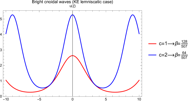
Figure 5: Bright cnoidal waves for the KE (1) with nonzero boundary conditions for $\alpha=1,\kappa=1$. When $c=1,2$ then $\beta=\frac{128}{507},\frac{64}{507}.$

IV Conclusion

In this paper we applied the generalized elliptic function method to find traveling wave solutions to Kawahara, transmission line, and Korteweg-de Vries equations, which has the advantage of finding solutions to nonlinear evolution equations as polynomial combinations of elliptic functions. Depending on the boundary conditions, these solutions can be reduced, if necessary, to the hyperbolic, periodic, or Jacobian elliptic functions.

By assuming a polynomial ansatz that satisfies an elliptic equation, in the case of KdV equation, we find the well-known solitary waves, as well as wave-trains of cnoidal waves which are either compressive or rarefactive that propagate in both directions with arbitrary velocity.

In the case of KE the traveling wave solutions are written in terms of Weierstrass elliptic functions which can be reduced to the hyperbolic (for zero boundary conditions) or Jacobi elliptic functions (for nonzero boundary conditions). For the general case the Weierstrass elliptic functions are unbounded, while for the lemniscatic case, they reduce to periodic cnoidal waves.

While for the KdV equation the solitary waves that are both compressive and rarefactive propagate with arbitrary velocity, for KE only compressive waves are found that propagate to one direction with a velocity that depends on both dispersion coefficients.

V Appendix

Lemma V.1.

Traveling wave solutions to KE (1), satisfy only the Weierstrass elliptic equation with cubic nonlinearity.

Proof.  Letting

$${Y_{\xi}}^{2}=\sum_{i=0}^{m}a_{i}Y^{i},\quad\quad a_{M}\neq 0.$$ (69)

For KdV Eq. (14) $u=Y$ and the leading term for the second order derivative term is $u_{\xi\xi}=\frac{1}{2}ma_{m}Y^{m-1}$. By matching the terms $u^{2}$ with $u_{\xi\xi}$ in Eq. (15) we obtain $m=3$. For KE (1) $u=Y^{2}$ and the leading term for the fourth order derivative term is $u_{\xi\xi\xi\xi}=\frac{1}{2}m(m+2)(3m-2){a_{m}}^{2}Y^{2(m-1)}$. By matching the terms $u^{2}$ and $u_{\xi\xi\xi\xi}$ in Eq. (7) we also obtain $m=3$. Notice that this method will not work if an ODE contains both even and odd derivative terms.

References

- (1) Ablowitz, Mark J., and Peter A. Clarkson. Solitons, nonlinear evolution equations and inverse scattering. Vol. 149. Cambridge University Press, Cambridge, U.K. (1991).
- (2) Abramowitz, Milton, and Irene A. Stegun. Handbook of mathematical functions: with formulas, graphs, and mathematical tables. Vol. 55. Courier Corporation. Washington, D.C. (1964).
- (3) Albert, John P. “Positivity properties and stability of solitary-wave solutions of model equations for long waves.” Comm. Partial Differential Equations 17 (1992):1-22.
- (4) Assas, Laila M.B. “New exact solutions for the Kawahara equation using Exp-function method.” Journal of Computational and Applied Mathematics 233.2 (2009): 97-102.
- (5) Baldwin, D., Göktaş, Ü., Hereman, W., Hong, L., Martino, R. S., and Miller, J. C. “Symbolic computation of exact solutions expressible in hyperbolic and elliptic functions for nonlinear PDEs.” Journal of Symbolic Computation 37.6 (2004): 669-705.
- (6) Cornejo-Pérez, O., Negro, J., Nieto, L. M., and Rosu, H. C. “Traveling-Wave Solutions for Korteweg-de Vries-Burgers Equations through Factorizations.” Foundations of Physics 36.10 (2006): 1587-1599.
- (7) Drazin, Philip G., and Robin S. Johnson. Solitons: an introduction. Vol. 2. Cambridge University Press, Cambridge, U.K. (1989).
- (8) Eremenko, Alexandre. “Meromorphic traveling wave solutions of the Kuramoto-Sivashinsky equation.” (preprint). arXiv:nlin/0504053 (2005).
- (9) Fan, Engui. “Multiple travelling wave solutions of nonlinear evolution equations using a unified algebraic method.” Journal of Physics A: Mathematical and General 35.32 (2002): 6853.
- (10) Fan, Engui. “Extended tanh-function method and its applications to nonlinear equations.” Physics Letters A 277.4 (2000): 212-218.
- (11) Fan, Engui, and Jian Zhang. “Applications of the Jacobi elliptic function method to special-type nonlinear equations.” Physics Letters A 305.6 (2002): 383-392.
- (12) Fu, Zuntao, Shikuo Liu, Shida Liu, and Qiang Zhao. “New Jacobi elliptic function expansion and new periodic solutions of nonlinear wave equations.” Physics Letters A 290.1 (2001): 72-76.
- (13) Hasimoto, H. “Water waves.” Kagaku 40 (1970): 401-408. In Japanese
- (14) Hereman, W., Banerjee, P. P., Korpel, A., Assanto, G., Van Immerzeele, A., and Meerpoel, A “Exact solitary wave solutions of nonlinear evolution and wave equations using a direct algebraic method.” Journal of Physics A: Mathematical and General 19.5 (1986): 607.
- (15) Hirota, Ryogo. “Exact solution of the Korteweg–de Vries equation for multiple collisions of solitons.” Physical Review Letters 27.18 (1971): 1192.
- (16) Kano, Kiyotsugu, and Toshio Nakayama. “An Exact Solution of the Wave Equation .” Journal of the Physical Society of Japan 50 (1981): 361.
- (17) Kakutani, Tsunehiko, and Hiroaki Ono. “Weak non-linear hydromagnetic waves in a cold collision-free plasma.” Journal of the Physical Society of Japan 26.5 (1969): 1305-1318.
- (18) Kawahara, Takuji. “Oscillatory solitary waves in dispersive media.” Journal of the Physical Society of Japan 33.1 (1972): 260-264.
- (19) Korteweg, Diederik Johannes, and Gustav De Vries. “XLI. On the change of form of long waves advancing in a rectangular canal, and on a new type of long stationary waves.” The London, Edinburgh, and Dublin Philosophical Magazine and Journal of Science 39.240 (1895): 422-443.
- (20) Kudryashov, Nikolay A. “Painlevé analysis and exact solutions of the Korteweg–de Vries equation with a source.” Applied Mathematics Letters 41 (2015): 41-45.
- (21) Kudryashov, Nikolai A. “On “new traveling wave solutions” of the KdV and the KdV-Burgers equations.” Communications in Nonlinear Science and Numerical Simulation 14.5 (2009): 1891-1900.
- (22) Kudryashov, Nikolai A. “A note on new exact solutions for the Kawahara equation using Exp-function method.” Journal of Computational and Applied Mathematics 234.12 (2010): 3511-3512.
- (23) Kudryashov, Nikolai A. “Meromorphic solutions of nonlinear ordinary differential equations.” Communications in Nonlinear Science and Numerical Simulation 15.10 (2010): 2778-2790.
- (24) Kudryashov, Nikolai A. “Simplest equation method to look for exact solutions of nonlinear differential equations.” Chaos, Solitons & Fractals 24.5 (2005): 1217-1231.
- (25) Kudryashov, Nikolai A.. “Exact solutions of the generalized Kuramoto-Sivashinsky equation.” Physics Letters A 147.5-6 (1990): 287-291
- (26) Kudryashov, Nikolai A. “A note on the -expansion method.” Applied Mathematics and Computation 217.4 (2010): 1755-1758.
- (27) Kudryashov, Nikolay A. “One method for finding exact solutions of nonlinear differential equations.” Communications in Nonlinear Science and Numerical Simulation 17.6 (2012): 2248-2253.
- (28) Liu, Shikuo, Zuntao Fua, Shida Liua and Qiang Zhao. “Jacobi elliptic function expansion method and periodic wave solutions of nonlinear wave equations.” Physics Letters A 289.1 (2001): 69-74.
- (29) Malfliet, Willy. “Solitary wave solutions of nonlinear wave equations.” American Journal of Physics 60.7 (1992): 650-654.
- (30) Malfliet, Willy, and Willy Hereman. “The Tanh method: I. Exact solutions of nonlinear evolution and wave equations.” Physica Scripta 54.6 (1996): 563-568.
- (31) Malfliet, Willy, and Willy Hereman. “The Tanh method: II. Perturbation technique for conservative systems.” Physica Scripta 54.6 (1996): 569-575.
- (32) Ma, Wen-xiu. “Travelling wave solutions to a seventh order generalized KdV equation.” Physics Letters A 180.3 (1993): 221-224.
- (33) Mancas, Stefan C., Greg Spradlin, and Harihar Khanal. “Weierstrass traveling wave solutions for dissipative Benjamin, Bona and Mahony (BBM) equation.” Journal of Mathematical Physics 54.8 (2013): 081502.
- (34) Mancas, Stefan C. and Ronald Adams. “ Elliptic solutions and solitary waves of a higher order KdV–BBM long wave equation.” Journal of Mathematical Analysis and Applications, Volume 452, Issue 2, (2017):1168-1181.
- (35) Miura, M. R. Bäcklund Transformation, Springer-Verlag, Berlin, (1978).
- (36) Nagashima, Hiroyuki. “Experiment on Solitary Waves in the Nonlinear Transmission Line Described by the Equation ”Journal of the Physical Society of Japan 47.4 (1979): 1387-1388.
- (37) Natali, Fábio. “A note on the stability for Kawahara-KdV type equations.” Applied Mathematics Letters 23 (2010): 591-596.
- (38) Newell, Alan C. “The inverse scattering transform.” Solitons. Springer Berlin Heidelberg, (1980):177-242.
- (39) Nickel, Julia. “Elliptic solutions to a generalized BBM equation.” Physics Letters A 364.3 (2007): 221-226.
- (40) Nizovtseva, I. G., Galenko P. K. , and Alexandrov D. V. “The hyperbolic Allen-Cahn equation: exact solutions.” Journal of Physics A: Mathematical and Theoretical 49.43 (2016): 435201.
- (41) Parkes, E. J., and B. R. Duffy. “An automated tanh-function method for finding solitary wave solutions to non-linear evolution equations.” Computer physics communications 98.3 (1996): 288-300.
- (42) Porubov, Alexey V. “Periodical solution to the nonlinear dissipative equation for surface waves in a convecting liquid layer.” Physics Letters A 221.6 (1996): 391-394.
- (43) Porubov, A. V. “Exact travelling wave solutions of nonlinear evolution equation of surface waves in a convecting fluid.” Journal of Physics A: Mathematical and General 26.17 (1993): L797.
- (44) Porubov, A. V., and D. F. Parker. “Some general periodic solutions to coupled nonlinear Schrödinger equations.” Wave motion 29.2 (1999): 97-109.
- (45) Reyes, Marco A., Gutièrrez-Ruiz, David, Mancas, Stefan C., and Rosu, Haret C. “Nongauge bright soliton of the nonlinear Schrödinger (NLS) equation and a family of generalized NLS equations.” Modern Physics Letters A 31.03 (2016): 1650020.
- (46) Rosenau, Philip. “A quasi-continuous description of a nonlinear transmission line.” Physica Scripta 34.6B (1986): 827.
- (47) Rosenau, Philip. “Dynamics of Dense Discrete Systems High Order Effects.” Progress of Theoretical Physics 79.5 (1988): 1028-1042.
- (48) Sajjadi, Shahrdad G., Mancas, Stefan C., and Drullion, Frederique. “Formation of three-dimensional surface waves on deep-water using elliptic solutions of nonlinear Schrödinger equation.” Advances and Applications in Fluid Mechanics 18.1 (2015): 81-112.
- (49) Otwinowski, M., R. Paul, and W. G. Laidlaw. “Exact travelling wave solutions of a class of nonlinear diffusion equations by reduction to a quadrature.” Physics letters A 128.9 (1988): 483-487.
- (50) Prelle, Myra Jean, and M. F. Singer. “Elementary first integrals of differential equations.” Transactions of the American Mathematical Society 279.1 (1983): 215-229.
- (51) Stokes, George G. “On the theory of oscillatory waves.” Trans. Cambridge Philos. Soc. 8 (1847): 441-473.
- (52) Wang, Mingliang. “Solitary wave solutions for variant Boussinesq equations.” Physics letters A 199.3-4 (1995): 169-172.
- (53) Wazwaz, Abdul-Majid. ”New travelling wave solutions of different physical structures to generalized BBM equation.” Physics Letters A 355.4 (2006): 358-362.
- (54) Weiss, John, Michael Tabor, and George Carnevale. “The Painlevé property for partial differential equations.” Journal of Mathematical Physics 24.3 (1983): 522-526.
- (55) Whittaker, Edmund T., and Watson, George N. “A course of modern analysis. Reprint of the fourth (1927) edition. ” Chap. XX. Cambridge University Press, Cambridge, U.K. (1958).
- (56) Yamamoto, Yosinori, and Éi Iti Takizawa. “On a solution on non-linear time-evolution equation of fifth order.” Journal of the Physical Society of Japan 50.5 (1981): 1421-1422.
- (57) Yan, Zhenya, and Hongqing Zhang. “New explicit solitary wave solutions and periodic wave solutions for Whitham-Broer-Kaup equation in shallow water.” Physics Letters A 285.5 (2001): 355-362.
- (58) Yuan, Juan-Ming, Jie Shen, and Jiahong Wu. “A dual-Petrov-Galerkin method for the Kawahara-type equations.” Journal of Scientific Computing 34.1 (2008): 48-63.
- (59) Zhang, Sheng. “Exp-function method for Klein-Gordon equation with quadratic nonlinearity.” Journal of Physics: Conference Series. Vol. 96. No. 1. IOP Publishing (2008):012002.