Seismic Electric Signals: A physical interconnection with seismicity
Abstract
By applying natural time analysis to the time series of earthquakes, we find that the order parameter of seismicity exhibits a unique change approximately at the date(s) at which Seismic Electric Signals (SES) activities have been reported to initiate. In particular, we show that the fluctuations of the order parameter of seismicity in Japan exhibits a clearly detectable minimum approximately at the time of the initiation of the SES activity observed almost two months before the onset of the Volcanic-seismic swarm activity in 2000 in the Izu Island region, Japan. To the best of our knowledge, this is the first time that, well before the occurrence of major earthquakes, anomalous changes are found to appear almost simultaneously in two independent datasets of different geophysical observables (geoelectrical measurements, seismicity). In addition, we show that these two phenomena are also linked closely in space.
I Introduction
Seismic Electric Signals (SES) (Varotsos and Alexopoulos, 1984a; Varotsos et al., 1996) are low frequency (Hz) transient changes of the electric field of the Earth that precede earthquakes. Several such transient changes detected within a short time are termed SES activity. A proper combination of the SES physical properties enables the determination of the epicenter and the magnitude of an impending earthquake (EQ) (Varotsos and Alexopoulos, 1984a, b; Varotsos and Lazaridou, 1991; Varotsos et al., 1993). In addition, the small earthquakes subsequent to the initiation of an SES activity, when analyzed in a new time domain termed natural time (see below), enable the determination of the occurrence time of an impending mainshock a few days to around one week in advance (Varotsos et al., 2001a; Sarlis et al., 2008; Varotsos et al., 2011a).
Despite the successful predictions of several mainshocks in Greece, for example all the mainshocks with moment magnitude 6.4 during the decade 2001-2011 (see subsections 7.2.1 to 7.2.6 of Varotsos et al., 2011a, as well as a few major mainshocks in areas previously considered aseismic, see Chapters 5 and 14 of Lazaridou-Varotsos 2013), the SES research has been a target of a heated debate, as noticed in a recent review by Uyeda et al. (2009a). It is the main objective of this paper to hopefully end this debate by reporting an important fact which unambiguously shows that the initiation of an SES activity is accompanied by a clearly detectable change in an independent geophysical dataset of different physical observables.To understand the issue, we first summarize below the pressure stimulated polarization currents (PSPC) model proposed by Varotsos and Alexopoulos (1986) (see also Varotsos et al., 1993) for the SES generation mechanism as well as recapitulate the up to date knowledge on the lead time of the SES activities.
The PSPC model for the SES generation mechanism, based on Solid State Physics aspects, is consistent with the widely accepted concept that the stress gradually increases in the future focal region of an EQ. When this stress reaches a critical value, a cooperative orientation of the electric dipoles (which are anyhow present in the focal area due to lattice defects in the ionic constituents of the rocks, cf. all solids including metals, insulators and semiconductors contain intrinsic and extrinsic defectsVarotsos and Miliotis (1974); Kostopoulos et al. (1975); Varotsos and Alexopoulos (1977); Varotsos (1980, 2008)) is attained, which leads to the emission of a transient electric signal that constitutes an SES (the cooperativity is a hallmark of criticality). Note that no external electric field is a prerequisite for this electric dipoles’ orientation, because in the case of inhomogeneous stress (which should occur during the EQ preparation stage) the effect of the applied stress gradient is similar to that of an electric field (see also Varotsos et al., 2001b). The validity of this SES generation mechanism is strengthened by the fact that the up to date experimental data of SES activities (along with their associated magnetic field variations) have been shown to exhibit infinitely ranged temporal correlations (Varotsos et al., 2003a, b; Varotsos et al., 2009), thus being in accord with the conjecture of critical dynamics. According to Uyeda et al. (2009a), the PSPC model is unique among other models in that SES would be generated spontaneously during the gradual increase of stress without requiring any sudden change of stress such as microfracturing. The up to date observations of SES activities in Japan (for example see Uyeda et al., 2002, 2009b) as well as in Mexico (see Ramírez-Rojas et al., 2011, and references therein) and in California (see Bernardi et al., 1991; Fraser-Smith et al., 1990, where magnetic field variations similar to those associated with the SES activities in Greece have been reported) have shown that their lead time is of the order of a few months, in agreement with earlier observations in Greece (Varotsos and Lazaridou, 1991; Varotsos et al., 1993; Varotsos et al., 2011a). Thus, the observations of SES activities in various countries reveal that before the occurrence of major earthquakes there is a crucial time scale of around a few months or so (up to around 5 months, see Varotsos et al., 2011a), in which the critical stress is attained. This may reflect that changes in the correlation properties of other associated physical observables like seismicity may become detectable at this time scale. It is exactly this aspect at which our present work is focused on. In other words, it is the objective of the present study to examine whether upon the initiation of the emission of an SES activity there exists also a noticeable change in the correlation properties of seismicity. To unveil such a change we employ here natural time analysis (see Section II) since it has been demonstrated (see Varotsos et al., 2011a, and references therein) that novel dynamic features hidden behind time series in complex systems emerge upon analyzing them in natural time.
II Natural time analysis and seismicity. Background.
Natural time analysis, introduced a decade ago (Varotsos et al., 2001a, 2002a, 2002b, 2003b, 2003a; Varotsos et al., 2007), has found applications in a large variety of diverse fields and the relevant results have been compiled in a recent monograph (Varotsos et al., 2011a). In the case of seismicity, in a time series comprising earthquakes, the natural time serves as an index for the occurrence of the -th earthquake. The combination of this index with the energy released during the -th earthquake of magnitude , i.e., the pair , is studied in natural time analysis. Alternatively, one studies the pair , where
| (1) |
stands for the normalized energy released during the -th earthquake. It has been found (Varotsos et al., 2001a, 2003b, 2003a; Varotsos et al., 2005; Varotsos et al., 2011a) that the variance of weighted for , designated by , which is given by
| (2) |
plays a prominent role in natural time analysis. Note that , and hence , for earthquakes is estimated through the usual relation (Kanamori, 1978)
| (3) |
Seismicity exhibits complex correlations in time, space and magnitude () that have been studied in numerous investigations (for example, see Bak et al., 2002; Lennartz et al., 2011; Lippiello et al., 2012; Sarlis and Christopoulos, 2012). The observed earthquake scaling laws (e.g. see Turcotte, 1997) are widely accepted to indicate the existence of phenomena closely associated with the proximity of the system to a critical point (Holliday et al., 2006; Sornette, 2000; Carlson et al., 1994; Xia et al., 2008). Here, we take the view that earthquakes are (non-equilibrium) critical phenomena, and employ the analysis in natural time , because in the frame of this analysis an order parameter for seismicity has been introduced. In particular, it has been explained (Varotsos et al., 2005) in detail (see also pp. 249-253 of Varotsos et al., 2011a) that the quantity given by Eq. (2) -or the normalized power spectrum in natural time as defined by Varotsos et al. (2001a, 2002a) for natural angular frequency - can be considered as an order parameter for seismicity since its value changes abruptly when a mainshock (the new phase) occurs, and in addition the statistical properties of its fluctuations resemble those in other nonequilibrium and equilibrium critical systems.
The value of the order parameter () itself plays a key role in identifying the occurrence time of a mainshock. This is so, because it has been found (Varotsos et al., 2001a; Sarlis et al., 2008; Varotsos et al., 2011a) that a mainshock occurs in a few days to one week after the value is recognized to have approached 0.070 in the natural time analysis of the seismicity subsequent to the initiation of an SES activity. This has been ascertained in several major mainshocks in various countries including Greece, Japan and USA (see Varotsos et al., 2011a, and references therein).
III The data analyzed and the procedure followed.
To achieve the goal of the present study we need two types of datasets. The one should be a clearly observed SES activity and the other an authoritative earthquake catalog that will include the time series of the earthquakes during the time period of the observation of this SES activity. In Greece, there are several pairs of such datasets since our continuous SES observations are lasting for almost 30 years. However, in order to make our presentation more objective, we intentionally consider datasets reported by other independent workers that are easily accessible from the international literature. Specifically we shall consider the well known SES activity published by Uyeda and coworkers (Uyeda et al., 2002, 2009b) that preceded the volcanic-seismic swarm activity in 2000 in the Izu Island region, Japan. This was a pronounced SES activity with innumerable signals that started almost two months prior to the swarm onset. (The precise date of its initiation was reported to be on 26 April 2000, but see also below.) This swarm was then characterized by Japan Meteorological Agency (JMA) as being the largest earthquake swarm ever recorded (Japan Meteorological Agency, 2000). Further, to meet our goal we analyzed in natural time the series of the earthquakes reported during this period by the JMA seismic catalog. In particular, we considered all EQs within the area N, E, which covers the whole Japanese region (for example see Tanaka et al., 2004). The seismic moment , which is proportional to the energy released during an EQ (this is the quantity of the -th event used in natural time analysis), was obtained from the magnitude reported in the JMA catalog by using the approximate formulae of Tanaka et al. (2004) that interconnect with . Setting a threshold to assure data completeness, there exist 52,718 EQs in the period from 1967 to the time of Tohoku EQ. This reflects that we have on the average EQs per month.
Concerning the procedure followed, we consider a sliding natural time window of fixed length comprising consecutive events. Starting from the first earthquake, we calculate the values using 6 to 40 consecutive events (cf. This natural time window is used here as well as in Varotsos et al. (2013), while in Sarlis et al. (2013, 2015) reaches values up to ). We next turn to the second earthquake, and repeat the calculation of . After sliding, event by event, through the whole natural time window, the computed values enable the calculation of their average value and their standard deviation that correspond to this natural time window of length . We then determine the variability of , i.e., the quantity defined (Sarlis et al., 2010) as
| (4) |
In order to simplify the discussion of our results we employ the following change (Varotsos et al., 2011b): For each earthquake in the seismic catalog, we calculate the values resulting when using the previous 6 to 40 consecutive earthquakes. Then, the hitherto obtained values for the earthquakes to were considered for the estimation of the variability for a natural time window length . The resulting value, labelled , was attributed to , the data of which was obviously not included in the estimation.
Since we are interested -as explained in the first Section- on time scales comparable to that of the lead time of an SES activity, after considering that in Japan we have EQs with per month, as mentioned, we employ here the following natural time window lengths: 100, 200, 300, and 400 earthquakes.
IV Results
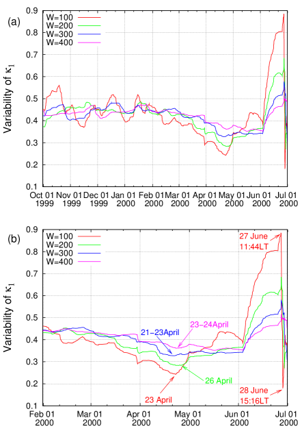
We first present the results of our analysis during nine months (see also the Appendix) until just before the occurrence of the 6.5 EQ on 1 July 2000 close to Niijima Island. During this period, i.e., 1 October 1999 to 1 July 2000, the four curves in Fig.1(a) depict the computed values of the variability of the order parameter for seismicity versus the conventional time (LT) for =100 (red), 200 (green), 300 (blue) and 400 (magenta). We see that the variability remains more or less constant until around 20 March 2000 and thereafter starts to decrease (note that Uyeda et al., 2009b, in their Fig. 11, have noticed that SES but of very small amplitude initiated approximately on 22 March). A clear minimum in the variability of is subsequently observed around the last week of April. To better visualize it, we now depict in expanded time scale an excerpt of Fig.1(a), see Fig.1(b), that refers only to the period from 1 February 2000 to 1 July 2000, i.e., during five months until just before the occurrence of the M6.5 EQ on 1 July 2000. An inspection of Fig.1(b) reveals that the minimum of the variability of is observed on the following date(s): 23 April for , 26 April for , 21-23 April for , and 23-24 April for (these dates are marked on the figure). For , 300, and 400, it seems that there is a tendency for the date of the minimum of to precede somewhat that of the initiation of the SES activity by a few days, but for the two dates coincide. In view of the experimental errors, however, mainly due to the earthquake magnitude determination, we cannot make an assertion on an exact coincidence of the two dates. In other words, under the current experimental uncertainty (of around a few days or so), we can say that our main finding points to the fact that the fluctuations of the order parameter of seismicity became minimum around (or at least very close to) the date (26 April) of the initiation of the SES activity reported by Uyeda et al. (2009b). A simple calculation shows that the probability of ascribing this almost simultaneous appearance of the two phenomena to chance, is very small if we just take into account that Fig.1(a) extends over a nine-month period (i.e., of the order of 1% even when considering a single value of ).
Note also that in Fig.1(b), after the beginning of June an increase of the variability becomes evident, but on 27 June 2000 (approximately at 11:44 LT) an abrupt decrease occurs. This may be understood in the following context: By setting natural time zero at the initiation time of the SES activity, Uyeda et al. (2009b) conducted the natural time analysis of seismic events in the rectangular region from to and from to depicted in the inset of Fig. 7. They found that on 27 June, the order parameter approached gradually, i.e., without significant fluctuations, see their Fig. 7(b) (in a similar fashion as observed repeatedly in the Greek cases, see Varotsos et al., 2001a) the value 0.070, thus signalling the imminent mainshock on 1 July 2000.
V The robustness of the co-location in time of the two phenomena with respect to the area selection
The aforementioned results were obtained as mentioned by analyzing in natural time the seismicity within the wide area 25-46oN 125-146oE,i.e., . In this section, we shall focus on studying how robust is the co-location in time of the two phenomena with respect to the choice of area selection. In other words, we shall present below an analysis that investigates how the date of the minimum of varies if the area selection is changed. Along these lines, we employ a sliding area window and determine the occurrences of the minimum of as a function of date. The analysis has been carried out for different sizes of the sliding area window.
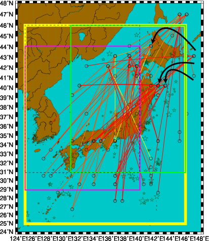
Before showing the present results of our analysis, we mention two earlier results. First, the wide area used here (surrounded by the yellow square in Fig.2) has been already employed by Varotsos et al. (2005, 2006) in order to show that the statistical properties of the fluctuations of the order parameter of seismicity resemble those in other nonequilibrium and equilibrium critical systems as already mentioned above in Section II. In particular, the properties of the probability density function (pdf) P versus -obtained by means of the procedure described in Section III- for the long term seismicity in the area were studied. It was found (Varotsos et al., 2005) that the scaled distribution PP plotted versus of this area falls on the same curve (universal) with the ones obtained from different seismic areas upon using the corresponding earthquake catalogs, e.g., Southern California (as well as that of the worldwide seismicity). This “universal” curve for the long term seismicity exhibits strikingly similar features (for example a common “exponential tail” characteristic of rare non-Gaussian fluctuations, e.g., of greater than six standard deviations from the mean) with the order parameter fluctuations in other nonequilibrium systems (e.g., 3D turbulent flow) as well as in several equilibrium critical systems (e.g., 2D Ising, 3D Ising). Second, we mention a study just published the findings of which will be of usefulness in an attempt towards understanding the results of our analysis that will be presented below. Specifically, Tenenbaum, Havlin, and Stanley (2012) proposed and developed a network approach to earthquake events. In this network, a node represents a spatial location while a link between two nodes represents similar activity patterns in the two different locations. The strength of a link is proportional to the strength of the cross-correlation in activities of two nodes joined by the link. They applied this network approach to the Japanese earthquake activity spanning the 14 year period 1985-1998 within an area that exceeds slightly (i.e., by in latitude and in longitude) the area used by our group. Tenenbaum et al. (2012) found strong links representing large correlations between patterns in locations separated by more than 1000 km. They found network characteristics not attributable to chance alone, including a large number of network links, high node assortativity, and strong stability over time. The network links (along with the corresponding nodes) identified by Tenenbaum et al. (2012), see their Fig.6(a), are superimposed on a map of the Japanese archipelago in Fig.2.
In the map of Fig.2, we also mark with green stars the epicenters of the 200 events when the ending of the natural time window of length 200 lies on the minimum of the variability marked in the green curve in Fig.1(b), i.e., on 26 April 2000. Let us now examine what happens with this date when our analysis is carried out for different sizes of the sliding area window (we follow, of course, the same procedure as in the wide area for =200, i.e., for each size we consider as the corresponding number of the events that would on average occur within two months). At the moment, we restrict ourselves to sizes which correspond to distances that markedly exceed the aforementioned distance of 1000 km. In particular, we present below examples for sliding area window sizes , and . The results obtained for the period 1 October 1999 to 1 July, 2000 (i.e., in a similar fashion as in Fig.1(a)) are as follows:
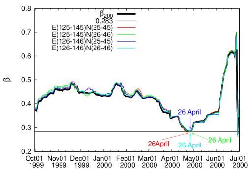
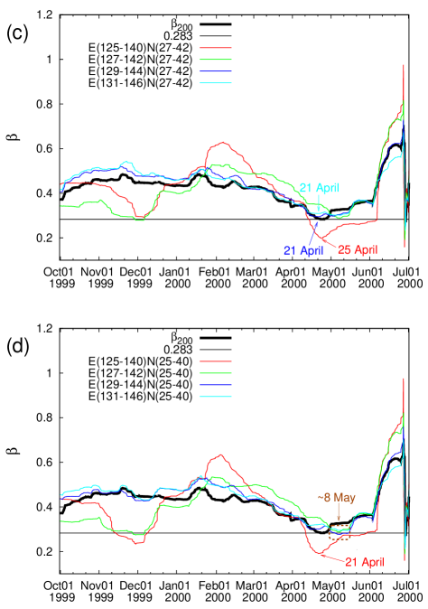
For the sliding area window , the resulting curves for the variability versus the conventional time for the four areas , , , and are shown in Fig.3 in red, green, blue and cyan, respectively. All these four curves exhibit a minimum on 26 April 2000, thus agreeing with the findings in the green curve in Fig.1 for 200 for the area . The curve for the latter case is also shown (thick black) in Fig.3 for the sake of comparison.
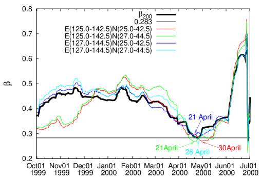
For the sliding area window the four areas investigated are the following: , , and leading to the corresponding curves plotted in Fig.4 in red, green, blue and cyan, respectively. They show that the minimum of is identified on the following dates: 30 April, 21 April, 21 April and 26 April 2000, respectively, which are more or less in agreement with the date(s) in Fig.1. By the same token as in Fig.3, we insert a thick black curve in Fig.4 showing the results plotted in Fig.1 for 200.
As a third example, we present the results for the sliding area window . In this case, the study included the investigation of sixteen areas -separated by in longitude and/or in latitude- the results of which are depicted in Figs.5(a), (b), (c) and (d). The coordinates of each of these areas are shown in the upper left corner in each figure, which also includes a thick black curve showing the result of the original area for 200 for the sake of comparison. The results could be summarized as follows: In ten areas (out of 16), we find that the minimum of appears at dates lying between 21 and 27 April 2000 (i.e., see the three cases marked in each of the figures 5(a), (b) and (c) as well as the one case marked in red in Fig.5(d)) and hence close to the date of 26 April 2000 observed in Fig.1 for 200). In four areas (out of 16) the minimum of appears somewhat shifted, i.e., around 8 May 2000 (these are the three cases marked with a brown box in Fig.5(d) and the green curve in Fig.5(c)). Two areas, however, i.e., and , the results of which are depicted in red in Figs.5(a) and (b), do not exhibit a minimum of close to the expected date of 26 April 2000. In an attempt to understand why these two areas behave differently compared to the other areas, they are shown in the map of Fig.2 with broken black and solid purple squares, respectively superimposed on the network links map identified by Tenenbaum et al. (2012). For the sake of comparison, we also show in the same figure, as an example, the area -see the rightmost green square in Fig.2- in which our analysis led to the conclusion that there exists a minimum in the variability on 26 April 2000, see the cyan curve in Fig.5(a), thus being in agreement with the date of the minimum (26 April) identified in Fig.1 (green curve) for 200. A careful inspection of Fig.2 reveals that a number of nodes - three of which are shown with arrows- associated with a multitude of links lie outside of the two areas and but inside the area .
VI Investigation on whether the two phenomena are linked also in space
To answer this important question, we must focus on an analysis similar to that presented in the previous Section, but to a sliding area window of appreciably smaller size. This size cannot be smaller than if we consider the following: In the whole area we have 200 events -covering almost two months- that preceded the minimum on 26 April 2000 shown in the green curve of Fig.1, hence an area window of corresponds on the average to events per two months. In addition, we have to take into account that in order to identify the date of the occurrence of the minimum of in an area window of size with an uncertainty of around a few days, we must have at least, on the average, 2 events per week; thus, in an area window we must have at least 16 events for an almost two months period (8 weeks).
An area window of size sliding through the area results in areas when varying the center of each area with steps of in longitude and/or in latitude. Among these 81 areas, we select those that have at least 16 events per two months and find the 23 areas the coordinates of which are given in Table 1 and depicted in Fig.6(a). By analyzing these 23 areas we find the following:
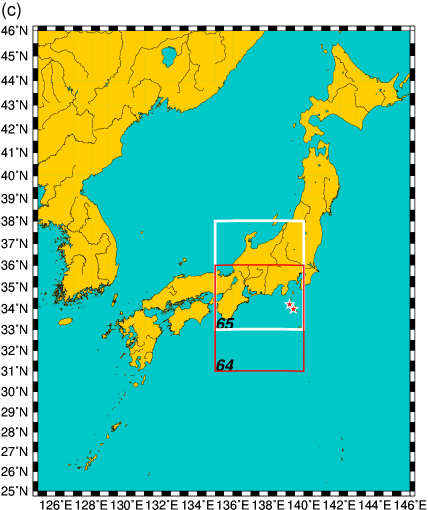
First, there exist only three areas labeled “65”, “87” and “97”, i.e., the ones with coordinates , and , that result in a clearly observable minimum of the variability the date of which differs by no more than a few days from the date 26 April 2000 exhibited in Fig.1 (green curve) for . In particular, the minimum in these three areas is observed on 25, 26, and 26 April, respectively, as shown in Fig.6(b) see the curves plotted in blue, green and cyan. Obviously, the lowest minimum is exhibited by the first area, i.e., , which remarkably includes the epicenters -marked with asterisks in Fig.6(c)- of the two earthquakes that occurred on 1 and 30 July 2000 close to Niijima Island measuring station (see also the inset of Fig.7).
Second, concerning the area labelled “64”, i.e., , which (also includes, see Fig.6(c), the epicenters of the aforementioned two EQs and) is somewhat displaced to the south compared to the area mentioned above, we observe the following: It exhibits a very shallow minimum of the variability around 15 April 2000, which however is almost a plateau extending up to 24 April 2000, hence being more or less close to the date (26 April) of the minimum observed in Fig.1 (green curve) for 200.
In other words, the findings of this Section, could be summarized as follows: Here, by using a narrow spatial window sliding through the wide () area , we investigated the earthquake events that would occur in an almost two months period. Recall that in the wide area these earthquakes have been interpreted (in the discussion of the minimum in the green curve of Fig.1) to correlate with the SES. We found that the characteristics of the fluctuations of (i.e., their lowest minimum) are linked to the seismicity occurring in the areas and that include the Izu Island region which became active a few months later.
VII Conclusions
Just by analyzing the Japanese seismic catalog in natural time, and employing a sliding natural time window comprising the number of events that would occur in a few months, we find the following: The fluctuations of the order parameter of seismicity exhibit a clearly detectable minimum approximately at the time of the initiation of the pronounced SES activity observed by Uyeda et al. (2002, 2009b) almost two months before the onset of the volcanic-seismic swarm activity in 2000 in the Izu Island region, Japan. This reflects that presumably the same physical cause led to both effects observed, i.e, the emission of the SES activity and the change of the correlation properties between the earthquakes. This might be the case when the stress reached its critical value, if we think in terms of the SES generation model proposed by Varotsos and Alexopoulos (1986). In addition, the two phenomena discussed are found to be also linked in space.
Finally, we note that the appearance of minima in the variability of before major earthquakes in Japan is investigated in detail elsewhere (Sarlis et al., 2013). For the vast majority of these cases, however, the main conclusion of the present investigation, i.e., the almost simultaneous appearance of these minima with the initiation of SES activities, cannot be checked due to the lack of geolectrical data. It is this lack of data which obliges us, as explained in the Appendix, to present in Fig. 1(a) the results of our analysis solely for a period of nine months, i.e., 1 October 1999 to 1 July 2000.
![[Uncaptioned image]](/html/1612.07056/assets/x5.png)
![[Uncaptioned image]](/html/1612.07056/assets/x7.png)
| Area label | LONG (oE) | LAT (oN) | Center of the area | Average Nr. of events |
|---|---|---|---|---|
| per 2 months | ||||
| 21 | 127-132 | 25-30 | 129.5E 27.5N | 17 |
| 22 | 127-132 | 27-32 | 129.5E 29.5N | 18 |
| 32 | 129-134 | 27-32 | 131.5E 29.5N | 16 |
| 64 | 135-140 | 31-36 | 137.5E 33.5N | 29 |
| 65 | 135-140 | 33-38 | 137.5E 35.5N | 33 |
| 73 | 137-142 | 29-34 | 139.5E 31.5N | 22 |
| 74 | 137-142 | 31-36 | 139.5E 33.5N | 40 |
| 75 | 137-142 | 33-38 | 139.5E 35.5N | 53 |
| 76 | 137-142 | 35-40 | 139.5E 37.5N | 35 |
| 77 | 137-142 | 37-42 | 139.5E 39.5N | 22 |
| 82 | 139-144 | 27-32 | 141.5E 29.5N | 20 |
| 83 | 139-144 | 29-34 | 141.5E 31.5N | 23 |
| 84 | 139-144 | 31-36 | 141.5E 33.5N | 38 |
| 85 | 139-144 | 33-38 | 141.5E 35.5N | 52 |
| 86 | 139-144 | 35-40 | 141.5E 37.5N | 48 |
| 87 | 139-144 | 37-42 | 141.5E 39.5N | 45 |
| 88 | 139-144 | 39-44 | 141.5E 41.5N | 37 |
| 89 | 139-144 | 41-46 | 141.5E 43.5N | 19 |
| 95 | 141-146 | 33-38 | 143.5E 35.5N | 25 |
| 96 | 141-146 | 35-40 | 143.5E 37.5N | 38 |
| 97 | 141-146 | 37-42 | 143.5E 39.5N | 44 |
| 98 | 141-146 | 39-44 | 143.5E 41.5N | 39 |
| 99 | 141-146 | 41-46 | 143.5E 43.5N | 22 |
Appendix A Additional comments on points discussed in the text.
An analysis similar to that shown in Fig. 1(a), is presented by Sarlis et al. (2013) for an appreciably longer period, i.e., from 1 January 1984 until the Tohoku earthquake on 11 March 2011. This is so, because the interconnection between the minima of the variability of the order parameter of seismicity and major earthquakes investigated by Sarlis et al. (2013) requires solely the knowledge of seismic data. On the other hand, to meet the purpose of the present study we need as mentioned both seismic and geoelectrical data. The lack of the latter data imposes certain constraints on our study that will become clear below.
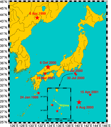
Figure 7 shows the epicenters (red stars) within the area 25-46oN 125-146oE of all EQs of magnitude comparable to or larger than that of the EQ on 1 July 2000 for a three year period from 1 January 1999 until 1 January 2002 extending from year before until year after the case discussed here. An inspection of this map reveals that eight EQs occurred, six of which had epicenters several hundreds kilometers away from the Niijima Island measuring station and two in its vicinity. Only the latter two EQs on 1 July 2000 and 30 July 2000 could have been preceded by SES activities recorded at Niijima station, in view of the up to date observations (Varotsos et al., 2011a) that magnitude 7.0 class EQs give detectable SES at epicentral distances up to around 250 km or so. In other words, the lack of geoelectrical data from stations that would have been installed in the regions surrounding the six distant EQs from Niijima Island, imposes the following constraint in order to achieve the goal of the present study: Only the analysis during the period preceding the occurrence of the two EQs in the neighborhood of Niijima Island (i.e., before 1 July 2000) could serve for the purpose of our study. Furthermore, and in order to avoid any influence on our results from the aftershock activity of the previous EQ that occurred on 8 April 1999 at 130.99oN 43.55oE of magnitude 7.1, we started our analysis some months later, i.e., on 1 October 1999 until just before the occurrence of the EQ on 1 July 2000. Nevertheless, despite this limitation imposed primarily from the lack of geoelectrical data at a multitude of measuring stations, we note the following privilege: The aforementioned SES activity at Niijima Island we considered here, is well isolated in time and space (since Uyeda et al., 2002, 2009b, noticed that, beyond the SES activity they reported, which started almost two months before the onset of the swarm activity, no other SES activities have been recorded at Niijima station either well before the onset or after the cessation of the swarm activity, e.g., see the caption of Fig. 9 of Uyeda et al. 2009b). This provides further convincing evidence in favor of our main finding and excludes any possibility of attributing it to chance, as already mentioned in the main text.
The following two comments are now in order:
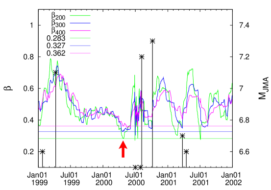
First, the analysis of the variability of of seismicity versus the conventional time, the results of which were presented as mentioned in Fig. 1(a) for the nine month period 1 October 1999 to 1 July 2000, was extended further into the past and the future. The relevant results during the three year period from 1 January 1999 to 1 January 2002 are now depicted in Fig. 8 for the three longer natural time window lengths =200, 300 and 400 events (the fluctuations of which are evidently appreciably smaller than those for =100 -see Fig. 1(a)- thus, if the latter were plotted in Fig. 8 it would overload this figure). For the sake of reader’s convenience, we also draw in Fig. 8 three horizontal lines that correspond to the minimum of the variability of , around the date 26 April 2000 (shown here by the thick red arrow), for =200 (green) =300 (blue) and =400 (magenta), respectively, already marked in Fig. 1(b). We clarify that, as already mentioned, the investigation of the interconnection of these minima with the subsequent major EQs, including the criteria that distinguish which of these minima are of truly precursory nature, was the objective of a separate study, see Sarlis et al. (2013), extended to an almost 27 year period (1984-2011). The aim of the present paper is, as already mentioned, essentially different: By focusing solely on the periods during which a pronounced SES activity has been recorded, as the one ( 26 April 2000) discussed here, to investigate whether there exists also an almost simultaneous change in the variability of of seismicity that is statistically significant.
Acknowledgements
We would like to express our sincere thanks to Professor H. Eugene Stanley, Professor Shlomo Havlin and Dr. Joel Tenenbaum for providing us the necessary data in order to insert in Fig. 2 the nodes and the associated links of their network.
References
- Varotsos and Alexopoulos (1984a) P. Varotsos and K. Alexopoulos, Tectonophysics 110, 73 (1984a).
- Varotsos et al. (1996) P. Varotsos, K. Eftaxias, M. Lazaridou, K. Nomicos, N. Sarlis, N. Bogris, J. Makris, G. Antonopoulos, and J. Kopanas, Acta Geophysica Polonica 44, 301 (1996).
- Varotsos and Alexopoulos (1984b) P. Varotsos and K. Alexopoulos, Tectonophysics 110, 99 (1984b).
- Varotsos and Lazaridou (1991) P. Varotsos and M. Lazaridou, Tectonophysics 188, 321 (1991).
- Varotsos et al. (1993) P. Varotsos, K. Alexopoulos, and M. Lazaridou, Tectonophysics 224, 1 (1993).
- Varotsos et al. (2001a) P. A. Varotsos, N. V. Sarlis, and E. S. Skordas, Practica of Athens Academy 76, 294 (2001a).
- Sarlis et al. (2008) N. V. Sarlis, E. S. Skordas, M. S. Lazaridou, and P. A. Varotsos, Proc. Jpn. Acad. Ser. B Phys. Biol. Sci. 84, 331 (2008).
- Varotsos et al. (2011a) P. A. Varotsos, N. V. Sarlis, and E. S. Skordas, Natural Time Analysis: The new view of time. Precursory Seismic Electric Signals, Earthquakes and other Complex Time-Series (Springer-Verlag, Berlin Heidelberg, 2011a).
- Lazaridou-Varotsos (2013) M. S. Lazaridou-Varotsos, Earthquake Prediction by Seismic Electric Signals: The success of the VAN method over thirty years (Springer Praxis Books, Berlin Heidelberg, 2013).
- Uyeda et al. (2009a) S. Uyeda, T. Nagao, and M. Kamogawa, Tectonophysics 470, 205 (2009a).
- Varotsos and Alexopoulos (1986) P. Varotsos and K. Alexopoulos, Thermodynamics of Point Defects and their Relation with Bulk Properties (North Holland, Amsterdam, 1986).
- Varotsos and Miliotis (1974) P. Varotsos and D. Miliotis, Journal of Physics and Chemistry of Solids 35, 927 (1974).
- Kostopoulos et al. (1975) D. Kostopoulos, P. Varotsos, and S. Mourikis, Can. J. Phys. 53, 1318 (1975).
- Varotsos and Alexopoulos (1977) P. Varotsos and K. Alexopoulos, J Phys. Chem. Solids 38, 997 (1977).
- Varotsos (1980) P. Varotsos, physica status solidi (b) 100, K133 (1980).
- Varotsos (2008) P. Varotsos, Solid State Ionics 179, 438 (2008).
- Varotsos et al. (2001b) P. Varotsos, V. Hadjicontis, and A. S. A.S. Nowick, Acta Geophysica Polonica 49, 415 (2001b).
- Varotsos et al. (2003a) P. A. Varotsos, N. V. Sarlis, and E. S. Skordas, Phys. Rev. E 67, 021109 (2003a).
- Varotsos et al. (2003b) P. A. Varotsos, N. V. Sarlis, and E. S. Skordas, Phys. Rev. E 68, 031106 (2003b).
- Varotsos et al. (2009) P. A. Varotsos, N. V. Sarlis, and E. S. Skordas, Chaos 19, 023114 (2009).
- Uyeda et al. (2002) S. Uyeda, M. Hayakawa, T. Nagao, O. Molchanov, K. Hattori, Y. Orihara, K. Gotoh, Y. Akinaga, and H. Tanaka, Proc. Natl. Acad. Sci. USA 99, 7352 (2002).
- Uyeda et al. (2009b) S. Uyeda, M. Kamogawa, and H. Tanaka, J. Geophys. Res. 114, B02310 (2009b).
- Ramírez-Rojas et al. (2011) A. Ramírez-Rojas, L. Telesca, and F. Angulo-Brown, Nat. Hazards Earth Syst. Sci. 11, 219 (2011).
- Bernardi et al. (1991) A. Bernardi, A. C. Fraser-Smith, P. R. McGill, and O. G. Villard, Phys. Earth Planet. Inter. 68, 45 (1991).
- Fraser-Smith et al. (1990) A. C. Fraser-Smith, A. Bernardi, P. R. McGill, M. E. Ladd, R. A. Helliwell, and O. G. Villard, Geophys. Res. Lett. 17, 1465 (1990).
- Varotsos et al. (2002a) P. A. Varotsos, N. V. Sarlis, and E. S. Skordas, Phys. Rev. E 66, 011902 (2002a).
- Varotsos et al. (2002b) P. A. Varotsos, N. V. Sarlis, and E. S. Skordas, Acta Geophysica Polonica 50, 337 (2002b).
- Varotsos et al. (2007) P. A. Varotsos, N. V. Sarlis, E. S. Skordas, and M. S. Lazaridou, Appl. Phys. Lett. 91, 064106 (2007).
- Varotsos et al. (2005) P. A. Varotsos, N. V. Sarlis, H. K. Tanaka, and E. S. Skordas, Phys. Rev. E 72, 041103 (2005).
- Kanamori (1978) H. Kanamori, Nature 271, 411 (1978).
- Bak et al. (2002) P. Bak, K. Christensen, L. Danon, and T. Scanlon, Phys. Rev. Lett. 88, 178501 (2002).
- Lennartz et al. (2011) S. Lennartz, A. Bunde, and D. L. Turcotte, Geophys. J. Int. 184, 1214 (2011).
- Lippiello et al. (2012) E. Lippiello, C. Godano, and L. de Arcangelis, Geophys. Res. Lett. 39, L05309 (2012).
- Sarlis and Christopoulos (2012) N. V. Sarlis and S.-R. G. Christopoulos, Chaos 22, 023123 (2012).
- Turcotte (1997) D. L. Turcotte, Fractals and Chaos in Geology and Geophysics (Cambridge University Press, Cambridge, 1997), 2nd ed.
- Holliday et al. (2006) J. R. Holliday, J. B. Rundle, D. L. Turcotte, W. Klein, K. F. Tiampo, and A. Donnellan, Phys. Rev. Lett. 97, 238501 (2006).
- Sornette (2000) D. Sornette, Critical Phenomena in the Natural Sciences: Chaos, Fractals, Selforganization, and Disorder: Concepts and Tools (Springer-Verlag, Berlin Heidelberg, 2000).
- Carlson et al. (1994) J. M. Carlson, J. S. Langer, and B. E. Shaw, Rev. Mod. Phys. 66, 657 (1994).
- Xia et al. (2008) J. Xia, H. Gould, W. Klein, and J. B. Rundle, Phys. Rev. E 77, 031132 (2008).
- Japan Meteorological Agency (2000) Japan Meteorological Agency, Earth Planets and Space 52, i (2000).
- Tanaka et al. (2004) H. K. Tanaka, P. A. Varotsos, N. V. Sarlis, and E. S. Skordas, Proc. Jpn. Acad. Ser. B Phys. Biol. Sci. 80, 283 (2004).
- Varotsos et al. (2013) P. A. Varotsos, N. V. Sarlis, E. S. Skordas, and M. S. Lazaridou, Tectonophysics 589, 116 (2013).
- Sarlis et al. (2013) N. V. Sarlis, E. S. Skordas, P. A. Varotsos, T. Nagao, M. Kamogawa, H. Tanaka, and S. Uyeda, Proc. Natl. Acad. Sci. USA 110, 13734 (2013).
- Sarlis et al. (2015) N. V. Sarlis, E. S. Skordas, P. A. Varotsos, T. Nagao, M. Kamogawa, and S. Uyeda, Proc. Natl. Acad. Sci. USA 112, 986 (2015).
- Sarlis et al. (2010) N. V. Sarlis, E. S. Skordas, and P. A. Varotsos, EPL 91, 59001 (2010).
- Varotsos et al. (2011b) P. Varotsos, N. Sarlis, and E. Skordas, EPL 96, 59002 (2011b).
- Varotsos et al. (2006) P. A. Varotsos, N. V. Sarlis, E. S. Skordas, H. K. Tanaka, and M. S. Lazaridou, Phys. Rev. E 74, 021123 (2006).
- Tenenbaum et al. (2012) J. N. Tenenbaum, S. Havlin, and H. E. Stanley, Phys. Rev. E 86, 046107 (2012).