Closed-form solution for the edge vortex of a revolving plate

Abstract

Flapping and revolving wings can produce attached leading edge vortices (LEVs) when the angle of attack is large. In this work, a low order model is proposed for the edge vortices that develop on a revolving plate at 90 degrees angle of attack, which is the simplest limiting case, yet showing remarkable similarity with the generally known LEVs. The problem is solved analytically, providing short closed-form expressions for the circulation and the position of the vortex. A good agreement with the numerical solution of the Navier–Stokes equations suggests that, for the conditions examined, the vorticity production at the sharp edge and its subsequent three-dimensional transport are the main effects that shape the edge vortex.

1 Introduction

Separated flows over flapping or revolving flat plates have gained attention over the past decades in the context of animal locomotion and insect flight in particular. Wings of insects have sharp edges that generate leading edge vortices (LEVs) responsible for the high lift coefficient at large angles of attack Ellington et al. (1996); Liu et al. (1998). The aerodynamics of flapping wings combines multiple lift-enhancement mechanisms. However, experiments with unilaterally rotating wings by Maxworthy (1979); Usherwood & Ellington (2002); Lentink & Dickinson (2009) have shown similar lift enhancement and LEV structures as flapping wings in the middle of downstroke and upstroke, and it has been recognized that the three-dimensional character of the flow is important therewith.

The shape of an LEV on a flapping or a revolving wing is approximately conical, it expands with the distance from the axis of revolution until it separates at some spanwise location where its size becomes commensurate with the wing local chord length Kruyt et al. (2015). The conical vortex leaves a triangular low-pressure footprint on the upper surface near the leading edge of the wing, thus producing net lift. This effect persists over a wide range of flow regimes, despite transitions from a steady laminar diffuse LEV when the Reynolds number is of order $Re=100$ to a more compact conical vortex core at $Re=1000$, then to a turbulent LEV at $Re$ of order $10000$ Usherwood & Ellington (2002); Garmann et al. (2013). It is likely that the spanwise flow from the wing root to the tip is critical for shaping up a steady LEV by removing the vorticity spanwise and depositing it into a trailing vortex Maxworthy (1979); Liu et al. (1998). Alternative explanations based on PIV measurements include the effect of downward flow induced by tip vortices Birch & Dickinson (2001) and vorticity annihilation due to interaction between the LEV and the opposite-sign layer on the wing Wojcik & Buchholz (2014).

As compared with the substantial amount of recent experimental and numerical work (for a review see, e.g., Limacher et al., 2016), only few analytical or low-order models have been proposed to understand the LEV dynamics of revolving wings. Maxworthy (2007) derived an estimate for the spanwise velocity. Limacher et al. (2016) studied the role of Coriolis accelerations. However, no estimate has been proposed for such an important quantity as the circulation. In §2 of the present paper, we derive closed-form expressions in elementary functions for the circulation and the position of the edge vortex. For simplicity, we restrict our attention to a rectangular plate at $90^{\circ}$ angle of attack. The edge vortex of this plate is nominally similar to the LEV of a plate at any large angle of attack, with the main difference of the downwash vanishing at the angle of $90^{\circ}$. Good agreement with the numerical solution of the incompressible Navier–Stokes equations shown in §3 suggests that, for the conditions examined, the vorticity production at the edge and its subsequent transport downstream and spanwise are likely the main effects that explain the circulation and the location of the vortices observed in the numerical simulations. Implications of these findings and perspectives for future improvement of the model are discussed in §4.

2 Mathematical formulation of the edge vortex model

The wing considered in this study is a flat plate with sharp edges. It is set at a constant angle of attack $90^{\circ}$ and revolves with a constant angular velocity $\Omega$ about the vertical axis, as shown in figure 1(a). For simplicity of the analysis, we suppose that the planar shape of the plate is rectangular with length $R$ and chord $c$, and that the axis of revolution passes through the root edge. Due to the top-bottom symmetry of the setup, we only focus on the flow above the symmetry plane, and the “edge vortex” refers to the vortex near the top edge of the plate, unless we explicitly state the opposite.

2.1 Line vortex model

Earlier studies have revealed a nominally conical shape of the edge vortex, which expands from the root towards the tip of the plate. In a reference frame revolving with the plate, the flow is essentially in the azimuthal direction and in the spanwise direction from the root to the tip. Therefore, the flow over the nearest sharp edge is likely to be the key factor that determines how the edge vortex develops over the proximal portion of the plate. The influence of the finite span of the plate only becomes strong near its distal part, and this effect is neglected in the present analysis. The effect of the finite chord length is taken into account approximately by using potential flow asymptotics for the velocity.

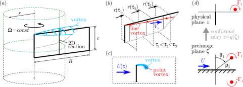
Figure 1: (a) Drawing of a revolving plate highlighting the edge vortex domain considered in our analysis. (b) Line vortex model and the radial position of a Lagrangian vortex element at consequent time instants $\tau_{1}$, $\tau_{2}$ and $\tau_{3}$. (c) Two-dimensional point vortex approximation of the flow. (d) The flow domain in the physical plane $z$ and in the preimage plane $\zeta$.

Thus, the viscous flow in a small neighborhood around the edge is dominated by the separation that produces vorticity. In two-dimensional flows, or if the plate is in pure translation, the vorticity accumulates in the near wake region until it sheds as a separated vortex. The flow topology changes dramatically due to the presence of the spanwise flow that removes the vorticity from the edge vortex and deposits it into a trailing vortex when the wing revolves Maxworthy (1979); Liu et al. (1998); Lentink & Dickinson (2009). Hence, among all of the effects that have any influence on the edge vortex properties, we postulate that two phenomena are of utter importance: (i) vorticity production and (ii) three-dimensional transport of the vorticity. Using approximate models of these two phenomena, we derive the desired estimates for the edge vortex position and circulation.

The next important step is to approximate the diffuse vortex core by a thin vortex line that originates from the root and extends toward the tip of the plate, see figure 1(b). An element $\mathrm{d}r$ of that line vortex at a distance $r$ from the axis of revolution substitutes for the radial vorticity in the fluid contained between two virtual cylinders of radii $r$ and $r+\mathrm{d}r$. Our model neglects the vorticity components in the directions other than the radial. The error is estimated a posteriori in Appendix A. We follow the path of a selected Lagrangian element of the line vortex as its distance from the axis of revolution $r(\tau)$ increases in time $\tau$ due to the spanwise advection, and use the Brown–Michael vortex to estimate the vorticity produced at any $r$. The Lagrangian vortex particle moves spanwise with the velocity $V_{r}$ such that $\mathrm{d}r/\mathrm{d}\tau=V_{r}(r)$. We postulate that it is related to the inflow velocity $U(r)$ as

$$V_{r}=K_{sp}U,\quad\mathrm{where}\quad U=\Omega r,$$ (1)

and earlier research by Maxworthy (2007) and Limacher et al. (2016), as well as our numerical simulations suggest that it is adequate to assume $K_{sp}=const$. After integration we obtain

$$r(\tau)=r_{0}e^{K_{sp}\Omega\tau}\quad\mathrm{and}\quad U(\tau)=\Omega r_{0}e^{K_{sp}\Omega\tau},$$ (2)

where $r_{0}$ is an integration constant. We thus reduce the three-dimensional steady problem to a two-dimensional unsteady problem of vortex dynamics on a cylinder of radius $r(\tau)$, and substitute it with a Brown–Michael model of the flow over a sharp edge, see figure 1(c). All three-dimensional effects other than the spanwise advection are neglected at this point.

2.2 Solution of the Brown–Michael model

The Brown–Michael model for the flow past a semi-infinite plate perpendicular to the free stream was solved by Cortelezzi (1995). We briefly repeat the derivation with only a slight modification of explicitly entering the chord length $c$ in the equation, for the ease of comparison with numerical simulations.

The physical flow domain is an infinite space with a vertical plate immersed in the fluid. The origin of the coordinate system $z=0$ is at the top edge of the plate. Using a conformal mapping

$$z=g(\zeta),\quad\textrm{where}~{}~{}g(\zeta)=-\mathrm{i}\zeta^{2}/c,$$ (3)

the leading-order term of the flow near the edge is mapped on the complex half-plane, as shown in figure 1(d). The point vortex has strength $\Gamma_{1}$ and position $z_{1}$ that vary in time $\tau$, and in the following we derive explicit solutions for these two quantities. Since it is obvious that the flow generates a clockwise vortex, we follow the convention of Cortelezzi (1995) that assumes that clockwise circulation is positive. The complex potential of the flow is equal to

$$W(\zeta,\tau)=U(\tau)\zeta-\frac{\Gamma_{1}(\tau)}{2\pi\mathrm{i}}\ln\frac{\zeta-\zeta_{1}(\tau)}{\zeta-\zeta_{1}^{*}(\tau)}.$$ (4)

The Kutta condition is satisfied if $\partial W/\partial\zeta=0$ at $\zeta=0$, which determines the circulation

$$\Gamma_{1}(\tau)=2\pi\mathrm{i}\frac{\zeta_{1}(\tau)\zeta_{1}^{*}(\tau)}{\zeta_{1}(\tau)-\zeta_{1}^{*}(\tau)}U(\tau).$$ (5)

The unknown position of the vortex $\zeta_{1}$ is obtained from the Brown–Michael equation

$$\frac{\mathrm{d}z_{1}^{*}}{\mathrm{d}\tau}+z_{1}^{*}\frac{1}{\Gamma_{1}}\frac{\mathrm{d}\Gamma_{1}}{\mathrm{d}\tau}=\tilde{u}^{*}$$ (6)

with $z^{*}_{1}(0)=0$ as the initial condition. The de-singularized complex conjugate velocity of the point vortex in the physical plane is equal to

$$\tilde{u}^{*}=\frac{\mathrm{i}c}{2\zeta_{1}}\left\{U(\tau)-\frac{\mathrm{i}\Gamma_{1}(\tau)}{2\pi}\frac{1}{\zeta_{1}(\tau)-\zeta_{1}^{*}(\tau)}-\frac{\mathrm{i}\Gamma_{1}(\tau)}{4\pi}\frac{g^{\prime\prime}(\zeta_{1}(\tau))}{g^{\prime}(\zeta_{1}(\tau))}\right\}.$$ (7)

After substituting (7), (5) and (3) into (6), we obtain an ordinary differential equation for $\zeta_{1}$,

$$\left(2\mathrm{i}\zeta_{1}^{*}+\frac{\mathrm{i}\zeta_{1}\zeta_{1}^{*}}{\zeta_{1}-\zeta_{1}^{*}}\right)\frac{\mathrm{d}\zeta_{1}^{*}}{\mathrm{d}\tau}-\frac{\mathrm{i}{\zeta_{1}^{*}}^{3}}{\zeta_{1}(\zeta_{1}-\zeta_{1}^{*})}\frac{\mathrm{d}\zeta_{1}}{\mathrm{d}\tau}+\frac{\mathrm{i}{\zeta_{1}^{*}}^{2}}{U}\frac{\mathrm{d}U}{\mathrm{d}t}=\frac{\mathrm{i}c^{2}}{2\zeta_{1}}\left(U-\frac{\mathrm{i}\Gamma_{1}}{2\pi(\zeta_{1}-\zeta_{1}^{*})}-\frac{\mathrm{i}\Gamma_{1}}{4\pi\zeta_{1}}\right)$$ (8)

with the initial condition $\zeta_{1}(0)=0$. In the polar coordinates $\rho_{1}$ and $\theta_{1}$ such that $\zeta_{1}=\rho_{1}e^{\mathrm{i}(\pi/2-\theta_{1})}$, equation (8) is equivalent to a system of two equations,

$$\begin{split}\frac{\mathrm{d}\rho_{1}}{\mathrm{d}\tau}&=\frac{c^{2}U}{12\rho_{1}^{2}}\sin\theta_{1}-\frac{\rho_{1}}{3U}\frac{\mathrm{d}U}{\mathrm{d}\tau},\\ \frac{\mathrm{d}\theta_{1}}{\mathrm{d}\tau}&=\frac{c^{2}U}{8\rho_{1}^{3}}\frac{\cos 2\theta_{1}}{\cos\theta_{1}}\end{split}$$ (9)

with the initial conditions

$$\begin{split}\rho_{1}(0)&=0,\\ \theta_{1}(0)&=\theta_{0},\quad\theta_{0}\in]-\pi/2,\pi/2[.\end{split}$$ (10)

After the change of variables $\Upsilon=U\rho_{1}^{3}/c^{2}$, $\Theta=\sin\theta_{1}$ and

$$\tilde{\tau}=\int_{-\infty}^{\tau}U^{2}(\tau^{\prime})\mathrm{d}\tau^{\prime}=\frac{\Omega r^{2}}{2K_{sp}}$$ (11)

that makes use of (2), equations (9) transform into

$$\frac{\mathrm{d}\Upsilon}{\mathrm{d}\tilde{\tau}}=\frac{\Theta}{4},\quad\frac{\mathrm{d}\Theta}{\mathrm{d}\tilde{\tau}}=\frac{1-2\Theta^{2}}{8\Upsilon}$$ (12)

with $\Upsilon(0)=0$ and $\Theta(0)=\Theta_{0}\in]-1,1[$. Combining the two equations, we obtain an equation of the second order,

$$\frac{\mathrm{d}^{2}(\Upsilon^{2})}{\mathrm{d}\tilde{\tau}^{2}}=\frac{1}{16},$$ (13)

that has two branches of the solution $\Upsilon=\pm\tilde{\tau}/\sqrt{32}$ satisfying the desired boundary condition, and we choose the ‘+’ sign which is the physically relevant one. We therefore find $\Theta=\sqrt{2}/2$ and

$$\rho_{1}=\left(\frac{c^{2}\tilde{\tau}}{2^{5/2}U}\right)^{1/3},\quad\theta_{1}=\frac{\pi}{4}.$$ (14)

Noting that $\tilde{\tau}/U=r/2K_{sp}$ and mapping the solution to the physical plane using (3), we obtain the position of the vortex as a function of distance $r$ from the axis of revolution,

$$\frac{z_{1}}{c}=\frac{1}{2^{7/3}K_{sp}^{2/3}}\left(\frac{r}{c}\right)^{2/3}.$$ (15)

Even though $z_{1}$ is a complex number by definition, the imaginary part of (15) is zero. The circulation is obtained from (5). In polar coordinates it simplifies to $\Gamma_{1}=\pi\rho_{1}U/\cos{\theta_{1}}$, yielding

$$\frac{\Gamma_{1}}{\Omega c^{2}}=\frac{\pi}{(4K_{sp})^{1/3}}\left(\frac{r}{c}\right)^{4/3}.$$ (16)

Equations (15) and (16) are the main results of this paper.

2.3 Numerical solution of the Navier–Stokes equations

For validation of the theoretical model, we employ established tools of the computational fluid dynamics (CFD). The incompressible three-dimensional Navier–Strokes equations are solved using a commercial finite-volume code ANSYS CFX 14.5. We consider a plate with the chord length $c=1$ mm and uniform thickness $0.02c$. The distance from the axis of revolution to the tip is equal to $R=6c$ in all numerical simulations except one which is described separately in the end of §3.1. The plate is immersed in a spherical inner domain of radius $10c$, and both rotate around the vertical axis with the angular velocity that gradually increases with time $t$ as $0.5\Omega(1-\cos(\pi t/t_{ac}))$ until it becomes equal to $\Omega$, then remains constant during all $t>t_{ac}$ (cf. Harbig et al., 2013). The acceleration time $t_{ac}$ is equal to $0.0835T$, where $T=2\pi/\Omega$. The outer stationary domain is a cuboid with its top, bottom and side far-field boundaries located at, respectively, $120c$, $120c$ and $80c$ away from the center of the inner spherical domain. The domains are discretized with hexahedron meshes of high quality, with the minimum grid spacing adjacent to the wall surface $\delta_{min}=0.1\sqrt{\nu c/\Omega R}$. The General Grid Interface (GGI) technique is applied to connect the two domains in a Multiple Frame of Reference (MFR), and a moving grid method is utilized in the inner domain. The grids have about 2.54 million cells in the simulations with $\Omega$ equal to $130$, $260$ and $520~{}\mathrm{s}^{-1}$. The case of $\Omega=1300~{}\mathrm{s}^{-1}$ requires 4.61 million cells to ensure the same accuracy. The Courant number is approximately equal to 1 in all simulations. The kinematic viscosity of the fluid is equal to $\nu=1.56\cdot 10^{-5}$ m²/s. The near field of the plate reaches a seemingly steady state by $t=0.8T$, therefore, instantaneous flow fields at that time instant are used for the comparison with the theoretical estimates.

3 Discussion

3.1 Comparison between the analytical and the numerical solutions

The output of our model is the circulation (16) and the position (15) of the vortex as functions of $r/c$. These are well defined quantities for a line vortex, but there exist many alternative definitions of a vortex when it has a diffuse core. For an objective comparison between the theoretical estimates and the CFD results, let us not restrict our attention to the vorticity in the core. Instead, since the flow over the plate at $90^{\circ}$ is symmetric, let us consider the circulation $\Gamma_{\Sigma}(r)$ obtained by integrating the radial vorticity component $\omega_{r}$ over the entire half-cylinder of radius $r$ above the symmetry plane shown with green dashed lines in figure 1(a). When using $\omega_{r}$ obtained from the CFD, the vertical extent of the domain is truncated at $L_{y}/2=10c$, yielding

$$\Gamma_{\Sigma}^{CFD}=\int_{0}^{2\pi}\int_{0}^{L_{y}/2}\omega_{r}r\mathrm{d}y\mathrm{d}\phi,$$ (17)

where $y$ is the vertical coordinate and $\phi$ is the azimuthal coordinate.

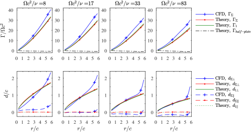
Figure 2: Comparison between the theoretical estimates and the CFD results for the circulation $\Gamma_{\Sigma}$ over a cylinder surface of radius $r$ (top row), and the distances between the edge and the vorticity centroids in the directions parallel and perpendicular to the plate, $d_{\parallel}$ and $d_{\perp}$, respectively (bottom row). Estimates for the point vortex circulation $\Gamma_{1}$, components of its distance to the edge $d_{1\perp}$, $d_{1\parallel}$, and the half-plate circulation $\Gamma_{half-plate}$ are added for reference. All quantities are normalized.

On the other hand, in the theoretical model, the line vortex substitutes for all vorticity in the entire domain with the exception of the boundary layers on the plate. The boundary layer vorticity is represented by the “bound” circulation along a contour that intersects with the plate but does not encompass the point vortex in the physical fluid domain. The bound circulation of a half-plate is estimated using the values of $W$ given by (4) at $c/2$ distance from the edge, on the pressure and on the suction side of the plate (see Appendix B for the derivation), resulting in

$$\frac{\Gamma_{half-plate}}{\Omega c^{2}}=\sqrt{2}\frac{r}{c}-\frac{\Gamma_{1}}{\Omega c^{2}}\left(\frac{1}{2}+\frac{1}{\pi}\arctan{\frac{1-2z_{1}/c}{2\sqrt{z_{1}/c}}}\right),$$ (18)

where $z_{1}$ is a real number, as given by (15). The theoretical estimate for $\Gamma_{\Sigma}(r)$ is therefore

$$\Gamma_{\Sigma}^{Theory}=\Gamma_{1}+\Gamma_{half-plate},$$ (19)

with the two components on the right-hand side evaluated using (16) and (18), respectively.

The top row panels in figure 2 present a comparison between $\Gamma_{\Sigma}^{Theory}$ and $\Gamma_{\Sigma}^{CFD}$ at different flow regimes characterized by the root-based Reynolds number $\Omega c^{2}/\nu$ in the range between 8 and 83. The equivalent Reynolds number based on the wing-tip velocity and the chord length $Re=\Omega Rc/\nu$ is in the range $Re=50...500$. All quantities are normalized. The agreement between the theoretical and the numerical results is good in all cases. The shape of the profiles makes the theoretical 4/3 power law apparent, while the good pointwise agreement is ensured by substituting $K_{sp}$ with a fit

$$\tilde{K}_{sp}=0.078\sqrt{\Omega c^{2}/\nu}$$ (20)

that minimizes the root mean square error, as discussed in the next section. Note that, even if $\tilde{K}_{sp}$ only depends on $\Omega c^{2}/\nu$, the dimensionless circulation (16) and position (15) depend on $r/c$ as well. It is straightforward, however, to derive a normalization that yields normalized $z_{1}$ and $\Gamma_{1}$ being functions of the root-based Reynolds number only: $z_{1}/(r^{2}c)^{1/3}=1.087(\Omega c^{2}/\nu)^{-1/3}$ and $\Gamma_{1}/\Omega(r^{2}c)^{2/3}=4.632(\Omega c^{2}/\nu)^{-1/6}$. Similar expressions can be written in terms of the local spanwise Reynolds number $\Omega rc/\nu$.

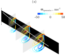
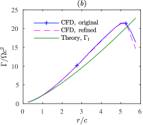
Figure 3: Flow over the plate at $\Omega c^{2}/\nu=83$. (a) Vorticity isocontours superposed with the theoretical position of the line vortex $z_{1}$. Vorticity magnitude scale is in milliseconds^-1. Gray shaded rectangles highlight the integration domain used for calculation of the vortex circulation in this example. (b) Normalized circulation of the vortex as a function of the normalized spanwise distance.

As $Re$ increases, $\Gamma_{\Sigma}$ becomes smaller. This is related to the vortex becoming nearer to the edge, as shown in the bottom row panels in figure 2, in terms of the components of the distance between the edge of the plate $z_{edge}$ and the vorticity central line $z_{\Sigma}$ in the directions perpendicular and parallel to the plate, $d_{\perp}=\Re(z_{\Sigma}-z_{edge})$ and $d_{\parallel}=\Im(z_{\Sigma}-z_{edge})$, respectively. The vorticity central line $z_{\Sigma}(r)$ in the CFD is calculated as

$$z_{\Sigma}^{CFD}=\frac{1}{\Gamma_{\Sigma}^{CFD}}\int_{0}^{2\pi}\int_{0}^{L_{y}/2}(r\phi+\mathrm{i}y)\omega_{r}r\mathrm{d}y\mathrm{d}\phi.$$ (21)

This definition is equally suitable for flows at any $Re$, including those cases when it is difficult to identify the vortex core. Its counterpart in the line vortex model is

$$z_{\Sigma}^{Theory}=\frac{z_{1}~{}\Gamma_{1}~{}+~{}z_{half-plate}~{}\Gamma_{half-plate}}{\Gamma_{1}+\Gamma_{half-plate}},$$ (22)

where $z_{half-plate}$ is calculated using the distribution of bound vorticity over the plate, as explained in Appendix B. The agreement between the theoretical estimate and the results of the numerical simulation is the best over the inner-central part of the plate. When $r/c>5$, the wing tip effects become dominant and the vorticity spreads far behind the plate in the CFD results. This effect is beyond the limitations of our theoretical model of the edge vortex that neglects aerodynamic interactions with the wing tip.

When $Re$ is sufficiently large, the edge vortex has a distinguishable core of large axial vorticity. Let us compare its properties with the line vortex model estimate at $\Omega c^{2}/\nu=83$. In PIV experiments as well as in numerical simulations, the circulation is usually calculated by summing up the spanwise vorticity contained in flat rectangular windows, cf. Carr et al. (2015). Therefore, in this example, we also use flat windows of hight $c$ and width $0.5r$, shown as gray shaded areas in figure 3(a). Sectional isolines of the vorticity component perpendicular to the integration planes reveal the vortex core. The white line superposed on the same figure shows the theoretical estimate (15) for the top edge vortex line. It passes through the vorticity core, which means that $z_{1}$ calculated using the line vortex model is a reasonable prediction for the apparent position of the vortex. Note that, even in 2D, the position of the point vortex does not exactly match the position of maximum vorticity (see Wang & Eldredge, 2013).

Figure 3(b) shows the normalized edge vortex circulation estimated by integration of the vorticity over the selected windows. CFD results obtained with two different discretization grids are shown: the original grid with 4.61 million cells and a refined grid with 9.96 million cells. The difference between these two results is less than 0.2% for all $r/c<5$, and only becomes noticeable near the tip where the wing tip vortex enters in the integration domain. The theoretical estimate for $\Gamma_{1}$ (16) is in a good agreement with the CFD results, with the difference being less than 17% for all $r/c<5$.

A remarkable property of the theoretical scaling law of $\Gamma_{1}$ with $r$ is that the exponent in (16) is independent of any parameters. It is therefore important to determine the best power law for fitting the CFD results. Therefore, we have carried out a two-parameter optimization of

$$\Gamma_{\Sigma}^{Fit}=A\left(\frac{r}{c}\right)^{B}$$ (23)

and determined the values of $A$ and $B$ that minimize the root-mean-square deviation with respect to $\Gamma_{\Sigma}^{CFD}$. The optimal values of $B$ are shown in figure 4. The mean value of $B$ over the considered range of $\Omega c^{2}/\nu$ is 1.32, which only differs by 1% from the theoretical estimate $4/3$ for the growth rate of $\Gamma_{1}$ with $r$.

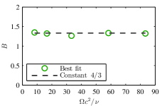
Figure 4: Optimal values of the power law exponent in $\Gamma_{\Sigma}^{Fit}$ that best-fit $\Gamma_{\Sigma}^{CFD}$ in the least-mean-squares sense.

The CFD data presented above is for a wing with the aspect ratio 6. The wing length does not enter in our theoretical estimate, but in the numerical simulation there may be some wing tip effects when the aspect ratio is small. We have carried out an additional numerical simulation of a wing with the chord length $2$ mm, i.e., twice as wide as the original plate. The angular velocity is equal to $\Omega=260$ s^-1. Apart from that, all parameters are the same. In particular, the wing length is equal to $6$ mm. The aspect ratio is therefore equal to 3. The root-based Reynolds number is equal to $\Omega c^{2}/\nu=67$. The comparison between the theoretical and the numerical results is shown in figure 5. The wing tip effects are significant over the distal part of the plate between $r/c=2$ and $3$. Importantly, the extent of that domain is similar to what we found in the case of aspect ratio 6. Over the proximal half of the plate, the agreement between the CFD results and the theory is good.

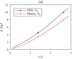
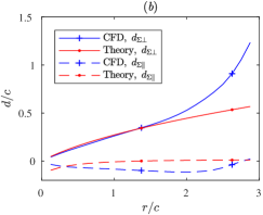
Figure 5: A plate with the aspect ratio equal to 3. Comparison between the theoretical estimates and the CFD results for (a) the circulation $\Gamma_{\Sigma}$ over a cylinder surface of radius $r$, and (b) the distances between the edge and the vorticity centroids in the directions parallel and perpendicular to the plate, $d_{\parallel}$ and $d_{\perp}$, respectively. All quantities are normalized.

3.2 Estimates of the average spanwise vorticity transport coefficient

The algebraic growth rate of $\Gamma_{1}$ as $r^{4/3}$ is fully defined by the line vortex model, but the prefactor in (16) contains a parameter $K_{sp}$ that determines how fast the Lagrangian elements of the line vortex are transported spanwise. We therefore refer to $K_{sp}$ as the spanwise vorticity transport coefficient. The exact value of $K_{sp}$ in each case depends on the distribution of the radial vorticity and the spanwise velocity in the flow field. Consequently, it depends on $Re$, for the reason that the structure of the edge vortex varies significantly with $Re$. Let us first derive a quick theoretical estimate of the spanwise vorticity transport coefficient $K_{sp}$ suitable for the low end of the range of $Re$ considered in the previous section. Let $V_{r}(r,\phi,y)$ be the radial velocity component in the cylindrical polar coordinates. At the plate, $\phi=0$ and the radial direction is aligned with the spanwise direction. The vorticity transport in the radial direction mainly takes place at those locations where both the radial vorticity $\omega_{r}$ and the radial velocity $V_{r}$ are large enough. To quantify it, we introduce the vorticity-weighted average radial velocity

$$\overline{V}_{r}(r,\Phi)=\frac{\int_{0}^{\Phi}\int_{0}^{Ly/2}V_{r}\omega_{r}r\mathrm{d}y\mathrm{d}\phi}{\int_{0}^{\Phi}\int_{0}^{L_{y}/2}\omega_{r}r\mathrm{d}y\mathrm{d}\phi}.$$ (24)

The parameter $\Phi\in[0,360^{\circ}]$ controls the extent of azimuthal averaging. Further, the CFD results suggest that $V_{r}$ is approximately linear in $r$ over the inner-central part of the plate. We therefore propose an estimate for the spanwise vorticity transport coefficient,

$$\overline{K}_{sp}=\overline{V}_{r}(r,\Phi)/\Omega r,$$ (25)

which we subsequently evaluate at a representative location $r_{ref}$. The overbar is to remind that the estimate is based on space averaging.

Near the plate, the vorticity is confined in two shear layers that start from the edges and propagate in the downstream direction. Due to the viscous exchange of momentum, the thickness of these vorticity sheets increases with the distance from the edges, and the peak vorticity magnitude decreases. We therefore use the one-dimensional diffusion equation in an unbounded domain to describe the evolution of the vorticity profiles with the angular distance $\phi$ from the plate. After introducing the time $t$ required for the plate to travel the angular distance $\phi$, the vorticity is approximated as

$$\omega_{r}(r,t,y)=\frac{\gamma(r)}{\sqrt{4\pi\nu t}}(e^{-\frac{(y-c/2)^{2}}{4\nu t}}-e^{-\frac{(y+c/2)^{2}}{4\nu t}}),\quad\mathrm{where}\quad t=\frac{\phi}{\Omega},$$ (26)

which satisfies the diffusion equation with the diffusivity equal to $\nu$, and the initial condition corresponding to delta distribution of the vorticity at the sharp edges.

The radial velocity is mainly driven by the centrifugal forces acting on the fluid trapped in the recirculation bubble, and it also decays with the distance away from the plate due to the action of viscosity. We assume the initial condition for $V_{r}$ of the form $V_{r}(r,0,y)=V_{r~{}max}(r)\left(1-4y^{2}/c^{2}\right)$, where, according to Maxworthy (2007), $V_{r~{}max}(r)=\sqrt{2}\Omega r$. The solution of the one-dimensional diffusion equation that satisfies the initial condition is

$$\begin{split}V_{r}(r,t,y)=V_{r~{}max}(r)\left\{\left(\frac{2}{c^{2}}(y^{2}+2\nu t)-\frac{1}{2}\right)\left(\operatorname{erf}{\frac{y-c/2}{\sqrt{4\nu t}}}-\operatorname{erf}{\frac{y+c/2}{\sqrt{4\nu t}}}\right)+\right.\\ \left.\frac{4}{c^{2}}\sqrt{\frac{\nu t}{\pi}}\left((y+\frac{c}{2})e^{-\frac{(y-c/2)^{2}}{4\nu t}}-(y-\frac{c}{2})e^{-\frac{(y+c/2)^{2}}{4\nu t}}\right)\right\}.\end{split}$$ (27)

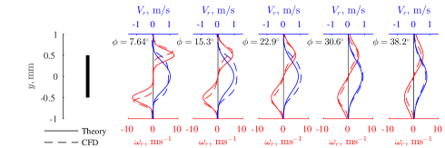
Figure 6: Line plots of the radial components of the vorticity $\omega_{r}$ (red) and the velocity $V_{r}$ (blue), sampled on vertical line segments between $y=-c/2$ and $y=c/2$, at a constant radial location $r_{ref}=3c$ and five different angular distances from the plate, $\phi=7.64^{\circ}n$, where $n=1,...,5$. The solid lines show the analytical profiles (26) and (27). The dash lines show the CFD results. Vorticity magnitude is in milliseconds^-1.

Sample profiles of $\omega_{r}$ and $V_{r}$ are shown in figure 6(a) and compared with the CFD data. They correspond to a plate revolving with the angular velocity $\Omega=260$ s^-1, i.e., $\Omega c^{2}/\nu=17$. The profiles are calculated at the radial location $r=3c$. The parameter $\gamma(r)$ is set to $2.7$ m/s when evaluating (26), but it cancels out in the subsequent calculation of $\overline{K}_{sp}$. The analytical profiles adequately describe the peaks of $\omega_{r}$ and $V_{r}$ as they flatten with the distance away from the plate. It should be reminded, however, that the analytical profiles do not account for the dynamic coupling between $\omega_{r}$ and $V_{r}$ and for many three-dimensional effects that may influence the rate of decay at larger $\phi$. In the following, we use them to obtain a rough order of magnitude approximation to $\overline{K}_{sp}$ that does not rely on any data from the CFD. On the other hand, to evaluate $\overline{K}_{sp}$ accurately, it is critical to account for the spatial distribution of $\omega_{r}$ and $V_{r}$ in all detail available from the CFD.

After substituting (26) and (27) into (24), performing numerical integration and substituting the result in (25), we obtain the desired theoretical estimate for $\overline{K}_{sp}$. The result does not depend on $r$ because $V_{sp~{}max}(r)$ is linear in $r$. Figure 7(a) compares the values of $\overline{K}_{sp}$ calculated using the profiles (26) and (27) with $\overline{K}_{sp}$ evaluated using $\omega_{r}$ and $V_{r}$ from the CFD at $r_{ref}=3c$. The plots are shown in a range of $\Phi$ to explore the sensitivity to this parameter. All values are within the interval between 0.23 and 0.4 when the linear distance from the plate is greater than $c$, i.e., $\Phi>19^{\circ}$. The general trend is a slow decrease with $\Phi$. The CFD result saturates at $\Phi>240^{\circ}$ when the numerator and the denominator in $\overline{V}_{r}$ in (24) attain their finite maximum values. The sudden drop at $\Phi=360^{\circ}$ is explained by the inward spanwise velocity on the pressure side of the plate previously reported by Kolomenskiy et al. (2014).

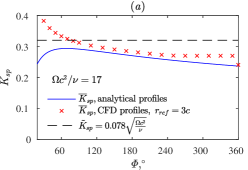
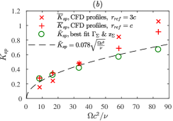
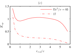
Figure 7: Estimates of the spanwise vorticity transport coefficient $K_{sp}$: (a) as a function of $\Phi$ at $\Omega c^{2}/\nu=17$, $\Phi$ being the upper limit of integration in (24); (b) as a function of the root-based Reynolds number $\Omega c^{2}/\nu$, with $\Phi=360^{\circ}$. (c) Spanwise distribution of the CFD-based estimate of the vorticity transport coefficient $\overline{K}_{sp}$, calculated as given by (24)-(25) with $\Phi=360^{\circ}$.

Figure 7(b) displays $K_{sp}$ as a function of the root-based Reynolds number $\Omega c^{2}/\nu$. In addition to the estimate $\overline{K}_{sp}$ obtained by integration of $V_{r}$ and $\omega_{r}$ from the CFD, the figure shows the values of $\tilde{K}_{sp}$ that best-fit the theoretical estimate to the CFD data in the least-mean-squares sense, i.e.,

$$\sqrt{\left(\frac{\Gamma_{\Sigma}^{Theory}-\Gamma_{\Sigma}^{CFD}}{\Gamma_{\Sigma}^{CFD}}\right)^{2}+\left(\frac{|z_{\Sigma}^{Theory}-z_{\Sigma}^{CFD}|}{|z_{\Sigma}^{CFD}|}\right)^{2}}\to\min.$$ (28)

A power law fit of those values leads to the empirical formula (20) that we used in the previous section. The agreement between these different estimates is good except for large $\Omega c^{2}/\nu$ and $r_{ref}$, when the discrepancy of up to 50% is caused by the vortex core structure becoming more complex and necessitating further investigation. Apart from that, the estimate $\overline{K}_{sp}$ is consistent with $\tilde{K}_{sp}$ that matches the observed circulation and location of the vortex.

Two sample spanwise distributions of $\overline{K}_{sp}$, obtained from the numerical simulations at $\Omega c^{2}/\nu=17$ and $83$, are shown in figure 7(c). In both cases, as postulated earlier, $\overline{K}_{sp}$ is roughly constant over the central part of the plate. Variation only becomes large near the ends of the plate, i.e., $r_{ref}<1c$ or $r_{ref}>4.5c$. Between these ends, the profile of $\overline{K}_{sp}$ depends on the Reynolds number: $\overline{K}_{sp}$ is monotonically decreasing when the Reynolds number is small, but it has a local maximum when the Reynolds number is large. Despite this small variability, the values sampled at $r_{ref}=1$ and $3$, used in figure 7(b), are representative of the average vorticity transport coefficient $\overline{K}_{sp}$ over the inner-central part of the plate that we need for the edge vortex circulation and position estimates.

Let us conclude this section with a comment on the physical mechanisms that drive the spanwise flow. This question has been extensively studied in the past research, and several different mechanisms have been proposed. Our objective is not to describe all factors that may have certain influence on the spanwise velocity $V_{r}$, but to quantify the role of $V_{r}$ in the vorticity dynamics. Our theoretical estimate (27) is based on the model proposed by Maxworthy (2007), who postulated that the centrifugal force and the outwards pressure gradient in the conical vortex core are the two equally important drivers of $V_{r}$. Other effects, such as the Coriolis acceleration and the wing-tip vortex induced velocity, that are not accounted for in our model, are likely to have less influence on $K_{sp}$ compared with the two main effects postulated above. For instance, the CFD computations by Garmann & Visbal (2014) with the centrifugal term eliminated from the Navier–Stokes equations show a dramatic decrease of the outwards spanwise velocity over the plate. Even though the peak outwards spanwise velocity in the vortex core is positive and may be an order of magnitude greater than the average Garmann & Visbal (2014); Limacher et al. (2016), it is the average velocity that apparently matters for $K_{sp}$ and for the edge vortex dynamics, as we infer from the overall good agreement between $\overline{K}_{sp}$ and $\tilde{K}_{sp}$ for the conditions examined.

3.3 Time evolution of the edge vortices

The solution derived in §2.2 is steady. However, the wing rotation starts from rest in our numerical simulations, as in many practical situations (such as the experiments by Carr et al., 2015, using rectangular wings operating at $45^{\circ}$ angle of attack and $Re$ of order several thousand). In addition to that, the flow may become unsteady due to hydrodynamic instabilities. It is therefore important to consider the time evolution of the edge vortex.

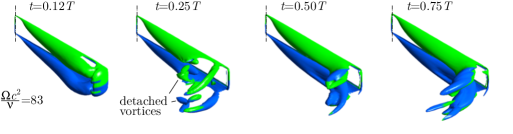
Figure 8: Instantaneous iso-surfaces of $\lambda_{2}=-10^{8}$ s^-2, colored according to the sign of the spanwise vorticity component, at four different time instants after startup. The root-based Reynolds number is equal to $\Omega c^{2}/\nu=83$.

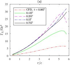
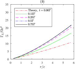
Figure 9: Time evolution of the circulation in the case $\Omega c^{2}/\nu=83$. (a) Values obtained from (17) using the CFD data; (b) Theoretical values of $\Gamma_{\Sigma}$ as given by (38).

Let us only discuss the largest Reynolds number case, $\Omega c^{2}/\nu=83$, which illustrates well different kinds of unsteady effects. The aspect ratio of the plate is equal to 6. We select the time instants at $0.12T$, $0.25T$, $0.5T$ and $0.75T$ for the flow visualization, where $T=2\pi/\Omega=4.8332\cdot 10^{-3}$ s. Time development of the vortex structure is illustrated by iso-surfaces of the $\lambda_{2}$-criterion in figure 8. In addition, we plot the normalized circulation as a function of the normalized spanwise distance in figure 9(a). The vortices over the proximal part of the plate, $r<3c$, reach steady state by the time $t=0.25T$. At the same time instant one can see a symmetric pair of counter-rotating vortices shed from the distal part of the plate, $r>4.5c$. Later, the flow becomes nominally steady over $r<4.5c$, but the wing-tip vortex is unsteady and small-scale eddies develop at this large Reynolds number.

Let us now amend our analysis to account for the gradual built-up of the edge vortex after the beginning of rotation. Let $t$ be physical time with $t=0$ at the startup. We extend the time profile of the plate angular velocity to negative $t$ as

$$\frac{\mathrm{d}\varphi_{plate}}{\mathrm{d}t}=\left\{\begin{aligned} &0,\quad t<0,\\ &\frac{\Omega}{2}(1-\cos\frac{\pi t}{t_{ac}}),\quad 0\leq t<t_{ac},\\ &\Omega,\quad t\geq t_{ac}.\end{aligned}\right.$$ (29)

Negative $t$ is the time before startup, when the plate and the surrounding fluid are at rest. Large positive $t>t_{ac}$ is when the plate revolves steadily. Note that, even though our solution is defined for any arbitrary large $t$, we are only interested in $t<T$ before the plate encounters its own wake from the previous revolution.

In the following analysis, the main difference with respect to the steady case is that now we track vortex particles over a physical time interval from the startup until a set time instant. The radial position $r$ of a tracer satisfies the evolution equation

$$\frac{\mathrm{d}r}{\mathrm{d}t}=K_{sp}\frac{\mathrm{d}\varphi_{plate}}{\mathrm{d}t}r.$$ (30)

Hence, the radial position of the tracer with the initial condition $r(0)=r_{0}$ can be written as

$$r=r_{0}e^{K_{sp}\hat{t}_{ac}g(s)/2},$$ (31)

where

$$\hat{t}_{ac}=\frac{\Omega t_{ac}}{\pi}=0.167,\quad s=\frac{\Omega t}{\hat{t}_{ac}},\quad\mathrm{and}\quad g(s)=\left\{\begin{aligned} &0,\quad s<0,\\ &s-\sin{s},\quad 0\leq s<\pi,\\ &2s-\pi,\quad s\geq\pi.\end{aligned}\right.$$ (32)

From the definition of $\tilde{\tau}$ (11) we obtain

$$\tilde{\tau}=\frac{\Omega r_{0}^{2}\hat{t}_{ac}}{4}\int_{-\infty}^{s}g_{s}^{2}(s^{\prime})e^{K_{sp}\hat{t}_{ac}g(s^{\prime})}\mathrm{d}s^{\prime},$$ (33)

where the subscript $\cdot_{s}$ stands for the derivative. Integration by parts yields

$$\tilde{\tau}=\frac{\Omega r_{0}^{2}}{4K_{sp}}\left\{\left.g_{s}(s^{\prime})e^{K_{sp}\hat{t}_{ac}g(s^{\prime})}\right|_{-\infty}^{s}-\int_{-\infty}^{s}g_{ss}(s^{\prime})e^{K_{sp}\hat{t}_{ac}g(s^{\prime})}\mathrm{d}s^{\prime}\right\}$$ (34)

We use a Taylor series approximation $e^{x}\approx 1+x$ for the exponential under the integral sign, and express $r_{0}$ in terms of $r$ using (31). We thus obtain

$$\frac{\tilde{\tau}}{\Omega c^{2}}=\frac{1}{4K_{sp}}\left(\frac{r}{c}\right)^{2}\left\{g_{s}(s)\left(1-e^{-K_{sp}\hat{t}_{ac}g(s)}\right)-K_{sp}\hat{t}_{ac}f(s)e^{-K_{sp}\hat{t}_{ac}g(s)}\right\},$$ (35)

where

$$f(s)=\left\{\begin{aligned} &0,\quad s<0,\\ &\frac{\sin{2s}}{4}+\sin{s}-s\sin{s}-\frac{s}{2},\quad 0\leq s<\pi,\\ &\pi/2,\quad s\geq\pi.\end{aligned}\right.$$ (36)

The rest of the derivation is similar to the steady case. We finally obtain the position of the vortex

$$\frac{z_{1}}{c}=\frac{1}{2^{7/3}K_{sp}^{2/3}}\left(\frac{r}{c}\right)^{2/3}\left\{1-\left(1+K_{sp}\hat{t}_{ac}\frac{f(s)}{g_{s}(s)}\right)e^{-K_{sp}\hat{t}_{ac}g(s)}\right\}^{2/3}$$ (37)

and its circulation

$$\frac{\Gamma_{1}}{\Omega c^{2}}=\frac{\pi}{(4K_{sp})^{1/3}}\left(\frac{r}{c}\right)^{4/3}\frac{g_{s}(s)}{2}\left\{1-\left(1+K_{sp}\hat{t}_{ac}\frac{f(s)}{g_{s}(s)}\right)e^{-K_{sp}\hat{t}_{ac}g(s)}\right\}^{1/3}.$$ (38)

The half-plate circulation $\Gamma_{half-plate}$ is calculated with the same formula as in the steady case, see Appendix B, but using the time-dependent $\Gamma_{1}$ (38).

The sum circulation $\Gamma_{\Sigma}^{Theory}=\Gamma_{1}+\Gamma_{half-plate}$ is shown in figure 9(b), for the same values of the aspect ratio and the Reynolds number as in the numerical simulation, and using $K_{sp}$ as given by (20). The trend of $\Gamma_{\Sigma}$ increasing in time until it saturates is similar to what we observe in the numerical simulation, but the theory predicts slightly smaller growth, and it does not account for the overshoot at $t=0.25T$ and $0.5T$ near the tip of the plate. For small $t$, the vortex circulation $\Gamma_{1}$ is small, and the largest contribution to $\Gamma_{\Sigma}^{Theory}$ is from the linear term $\sqrt{2}r/c$ in the half-plate bound circulation $\Gamma_{half-plate}$ (18). As $t$ becomes large, the $r^{4/3}$ power law becomes dominant. Similar trends were found in the experiments by Carr et al. (2015).

4 Conclusions and perspectives

We have derived closed-form expressions for the edge vortex circulation $\Gamma_{1}$ and its position $z_{1}$, (16) and (15), respectively, of a revolving plate at $90^{\circ}$ angle of attack. The model only contains one free parameter, the spanwise vorticity transport coefficient $K_{sp}$. For the latter, we have proposed a crude theoretical estimate (25) and a practical fit (20) that minimizes the error of the circulation $\Gamma_{\Sigma}$. The theoretical estimates of $\Gamma_{\Sigma}$ and $z_{\Sigma}$ are in a good agreement with the numerical solution of the Navier–Stokes equations in the root-based Reynolds number range $\Omega c^{2}/\nu$ from 8 to 83. Remarkably, the growth rate of $\Gamma_{1}$ as $r^{4/3}$ is independent of any parameters. The vorticity production at the edge and its three-dimensional transport are therefore sufficient to describe the edge vortex circulation, to the leading order. Our model is not intended to explain the mechanisms that drive the spanwise flow, but the values of $K_{sp}$ that we obtain are consistent with the theory by Maxworthy (2007).

The flow considered in our study is similar to the LEV on a wing that operates at any large angle of attack. Generalization of (16) and (15) appears feasible, but special care should be taken of the downwash which is not present in the current model, which may require numerical solution of the Brown–Michael equation (6) and is therefore beyond the scope of this paper. Likewise, the effect of non-zero distance between the wing root and the axis of rotation (also known as petiolation, see Phillips et al., 2017) may lend itself to modelling using the same vortex method, with special care taken of the flow near the wing root. Finally, we emphasize that the mechanisms of stable attachment of LEVs are not well understood yet. The success of the Brown–Michael vortex model to describe the edge vortex of a revolving plate, confirmed in the present study, opens a new perspective to analyze the stability of the leading-trailing vortex pair and the transition to periodic vortex shedding, using methods similar to those developed by Michelin & Llewellyn Smith (2009).

The authors thank Jean-Yves Andro and Keith Moffatt for many enlightening discussions that ultimately led to this study, and Jeff Eldredge for his useful comments during the Thirteenth International Conference on Flow Dynamics. DK gratefully acknowledges the financial support from the JSPS (Japan Society for the Promotion of Science) Postdoctoral Fellowship, JSPS KAKENHI No. 15F15061. DC was partly supported by a JASSO Honors Scholarship. HL was partly supported by the JSPS KAKENHI No. 24120007 for Scientific Research on Innovative Areas. This work is dedicated in memory of Tony Maxworthy.

Appendix A Error of the local point vortex approximation

The rightmost term in (4) is the complex potential of a point vortex and its mirror image. A point vortex is a two-dimensional approximation for a straight line vortex in the three-dimensional flow that has constant circulation. However, in our three-dimensional model, the circulation varies as $r^{4/3}$. Therefore, the Kutta condition is not exactly satisfied. With the shape of the vortex line and its circulation given by (15) and (16), respectively, it is straightforward to use the Biot–Savart formula to compute the induced velocity at the edge of the plate. In figure 10(a), it is compared with the induced velocity in the local two-dimensional approximation. The relative difference is less than 20% in the range of $r/c$ between 0.3 and 4 in the examples considered in this paper.

A more significant error is to neglect the influence of the vortex generated by the bottom edge of the plate. If the vertical velocity component induced by the top edge vortex is $v_{top}=\Gamma_{1}/2\pi z_{1}$ (the imaginary part of $z_{1}$ in (15) is zero), then the vertical velocity component induced by the bottom edge vortex at the same point is $v_{bottom}=\Gamma_{1}z_{1}/2\pi(c^{2}+z_{1}^{2})$. The ratio between the magnitudes of $v_{bottom}$ and $v_{top}$ is shown in figure 10(b). For the largest Reynolds number, the ratio is of about 40% at most, it is less than 20% over the proximal half of the wing, and 21% on average over the span. For the lowest Reynolds number, it is 50% on average over the span. This effect may explain larger discrepancy in the position of the vortex found in the comparison with the CFD results at low Reynolds numbers.

When the circulation of the radial vortex line varies over its length, longitudinal vortices are produced such that the vortex system satisfies the Helmholtz theorems. In particular, this effect explains the wing tip vortices. The strength of the longitudinal vortices is related to the rate of change of the edge vortex circulation with $r$, therefore, their effect is likely to be of the same order of magnitude as that of the non-uniform distribution of the circulation. Detailed analysis of the three-dimensional wake is beyond the scope of this paper. Note that the original model developed by Brown & Michael (1954) also applied the two-dimensional approximation to solve a three-dimensional problem, which was the LEV of a delta wing in that case.

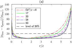
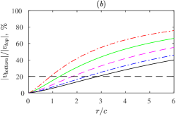
Figure 10: (a) Relative difference between the induced velocity of a line vortex of variable strength and a two-dimensional point vortex. (b) Vertical velocity magnitude due to the bottom-edge vortex relative to the velocity magnitude due to the top-edge vortex probed at the top edge.

Appendix B Bound circulation of the plate

The bound circulation corresponds to the vorticity contained in the boundary layers of the plate. Let us calculate the circulation $\Gamma_{b}(\delta,\tau)$ along a contour in the physical plane that begins at the pressure surface at a distance $\delta$ from the edge, wraps around the edge but not the point vortex in the fluid domain, and ends at the suction surface at the same distance $\delta$ from the edge. The beginning and the end points of the contour are, respectively, $z_{-}=\lim_{\epsilon\to 0}(-\epsilon-\mathrm{i}\delta)$ and $z_{+}=\lim_{\epsilon\to 0}(\epsilon-\mathrm{i}\delta)$, where $\epsilon\in\mathbb{R}^{+}$. The direction is consistent with our sign convention for the circulation. Knowing the complex potential (4), the bound circulation is equal to

$$\Gamma_{b}(\delta,\tau)=\Re\left\{W\left(\zeta(z_{+}),\tau\right)-W\left(\zeta(z_{-}),\tau\right)\right\}.$$ (39)

Noting that $\zeta(z_{+})=\sqrt{c\delta}$ and $\zeta(z_{-})=-\sqrt{c\delta}$, we obtain

$$\frac{\Gamma_{b}(\delta,\tau)}{\Omega c^{2}}=2\frac{r}{c}\sqrt{\frac{\delta}{c}}-\frac{\Gamma_{1}}{\Omega c^{2}}\frac{1}{\pi}\left\{\mathrm{Arg}\left(\sqrt{c\delta}-\zeta_{1}\right)-\mathrm{Arg}\left(-\sqrt{c\delta}-\zeta_{1}\right)+\pi n\right\},~{}~{}n\in\mathbb{Z}.$$ (40)

The value of $n$ is determined by requiring $\Gamma_{b}$ to be continuous with respect to $\delta$ and vanishing as $\delta\to 0$. After expressing $\mathrm{Arg}$ in terms of trigonometric functions and using the fact that $z_{1}$ is real, we find

$$\frac{\Gamma_{b}(\delta,\tau)}{\Omega c^{2}}=2\frac{r}{c}\sqrt{\frac{\delta}{c}}-\frac{\Gamma_{1}}{\Omega c^{2}}\left\{\frac{1}{2}+\frac{1}{\pi}\arctan{\frac{\delta-z_{1}}{\sqrt{2\delta z_{1}}}}\right\}.$$ (41)

In this work, we use (41) evaluated at $\delta=c/2$ as an approximation to the bound circulation of the upper half of a finite plate of chord $c$, i.e., $\Gamma_{half-plate}\approx\Gamma_{b}(c/2,\tau)$. This is consistent with the original semi-infinite plate assumption of this study. More accurate account of the bound vorticity distribution over a finite plate is possible, but in general it requires numerical integration. Though it may change the result quantitatively by as much as 41% (in the limiting case of $\Gamma_{1}=0$) comparing with the above estimate at $\delta=c/2$, the qualitative trends are not changed. Since $\Gamma_{half-plate}$ is, in practice, small compared with $\Gamma_{1}$, the approximation is adequate.

The position of the half-plate bound vorticity center is defined as

$$z_{half-plate}=-\mathrm{i}\delta_{half-plate},$$ (42)

where $\delta_{half-plate}$ is the distance from the edge of the plate to the half-plate bound vorticity center,

$$\delta_{half-plate}=\frac{1}{\Gamma_{half-plate}}\int_{0}^{c/2}{\delta\frac{\mathrm{d}\Gamma_{b}}{\mathrm{d}\delta}\mathrm{d}\delta}.$$ (43)

Taking the derivative of (41), we obtain

$$\frac{\mathrm{d}\Gamma_{b}}{\mathrm{d}\delta}=\Omega r\sqrt{\frac{c}{\delta}}-\frac{\Gamma_{1}}{\pi}\sqrt{\frac{z_{1}}{2\delta}}\frac{z_{1}+\delta}{z_{1}^{2}+\delta^{2}}.$$ (44)

From (42), (43) and (44), dividing the result by $c$, we obtain the normalized position of the half-plate bound vorticity center,

$$\frac{z_{half-plate}}{c}=-\mathrm{i}\frac{\frac{1}{3\sqrt{2}}\frac{r}{c}-\frac{\Gamma_{1}}{\Omega c^{2}}\frac{z_{1}}{\pi c}\left(\frac{1}{2}\log{\frac{\frac{1}{2}+\frac{z_{1}}{c}-\sqrt{\frac{z_{1}}{c}}}{\frac{1}{2}+\frac{z_{1}}{c}+\sqrt{\frac{z_{1}}{c}}}}+\sqrt{\frac{c}{z_{1}}}\right)}{\sqrt{2}\frac{r}{c}-\frac{\Gamma_{1}}{\Omega c^{2}}\left(\frac{1}{2}+\frac{1}{\pi}\arctan{\frac{1-2z_{1}/c}{2\sqrt{z_{1}/c}}}\right)}.$$ (45)

References

- Birch & Dickinson (2001) Birch, J. M. & Dickinson, M. H. 2001 Spanwise flow and the attachment of the leading-edge vortex on insect wings. Nature 412 (6848), 729–733.
- Brown & Michael (1954) Brown, C. E. & Michael, W. H. 1954 Effect of leading-edge separation on the lift of a delta wing. Journal of the Aeronautical Sciences 21 (10), 690–694.
- Carr et al. (2015) Carr, Z. R., DeVoria, A. C. & Ringuette, M. J. 2015 Aspect-ratio effects on rotating wings: circulation and forces. Journal of Fluid Mechanics 767, 497–525.
- Cortelezzi (1995) Cortelezzi, L. 1995 On the unsteady separated flow past a semi-infinite plate: Exact solution of the Brown and Michael model, scaling, and universality. Physics of Fluids 7 (3), 526.
- Ellington et al. (1996) Ellington, C. P., van den Berg, C., Willmott, A. P. & Thomas, A. L. R. 1996 Leading-edge vortices in insect flight. Nature 384 (6610), 626–630.
- Garmann & Visbal (2014) Garmann, D. J. & Visbal, M. R. 2014 Dynamics of revolving wings for various aspect ratios. Journal of Fluid Mechanics 748, 932–956.
- Garmann et al. (2013) Garmann, D. J., Visbal, M. R. & Orkwis, P. D. 2013 Three-dimensional flow structure and aerodynamic loading on a revolving wing. Physics of Fluids 25 (3), 034101.
- Harbig et al. (2013) Harbig, R. R., Sheridan, J. & Thompson, M. C. 2013 Reynolds number and aspect ratio effects on the leading-edge vortex for rotating insect wing planforms. Journal of Fluid Mechanics 717, 166–192.
- Kolomenskiy et al. (2014) Kolomenskiy, D., Elimelech, Y. & Schneider, K. 2014 Leading-edge vortex shedding from rotating wings. Fluid Dynamics Research 46, 031421.
- Kruyt et al. (2015) Kruyt, J. W., van Heijst, G. F., Altshuler, D. L. & Lentink, D. 2015 Power reduction and the radial limit of stall delay in revolving wings of different aspect ratio. Journal of The Royal Society Interface 12 (105), 20150051.
- Lentink & Dickinson (2009) Lentink, D. & Dickinson, M. H. 2009 Rotational accelerations stabilize leading edge vortices on revolving fly wings. The Journal of experimental biology 212, 2705–2719.
- Limacher et al. (2016) Limacher, E., Morton, C. & Wood, D. 2016 On the trajectory of leading-edge vortices under the influence of coriolis acceleration. Journal of Fluid Mechanics 800, R1.
- Liu et al. (1998) Liu, H., Ellington, C. P., Kawachi, K., van den Berg, C. & Willmott, A. P. 1998 A computational fluid dynamic study of hawkmoth hovering. Journal of Experimental Biology 201 (4), 461–477.
- Maxworthy (1979) Maxworthy, T. 1979 Experiments on the Weis-Fogh mechanism of lift generation by insects in hovering flight. Part 1. Dynamics of the ‘fling’. Journal of Fluid Mechanics 93 (1), 47–63.
- Maxworthy (2007) Maxworthy, T. 2007 The formation and maintenance of a leading-edge vortex during the forward motion of an animal wing. Journal of Fluid Mechanics 587 (2007), 471–475.
- Michelin & Llewellyn Smith (2009) Michelin, S. & Llewellyn Smith, S. G. 2009 An unsteady point vortex method for coupled fluid–solid problems. Theoretical and Computational Fluid Dynamics 23 (2), 127–153.
- Phillips et al. (2017) Phillips, N., Knowles, K. & Bomphrey, R. J. 2017 Petiolate wings: effects on the leading-edge vortex in flapping flight. Interface Focus 7 (1), 20160084.
- Usherwood & Ellington (2002) Usherwood, J. R. & Ellington, C. P. 2002 The aerodynamics of revolving wings II. Propeller force coefficients from mayfly to quail. Journal of Experimental Biology 205 (11), 1565–1576.
- Wang & Eldredge (2013) Wang, C. & Eldredge, J. D. 2013 Low-order phenomenological modeling of leading-edge vortex formation. Theoretical and Computational Fluid Dynamics 27 (5), 577–598.
- Wojcik & Buchholz (2014) Wojcik, C. J. & Buchholz, J. H. J. 2014 Vorticity transport in the leading-edge vortex on a rotating blade. Journal of Fluid Mechanics 743, 249–261.