Perturbative O($a^{2}$) effects in gradient flow couplings with SF and SF-open boundary conditions

Abstract:

The gradient flow provides a new class of renormalized observables which can be measured with high precision in lattice simulations. In principle this allows for many interesting applications to renormalization and improvement problems. In practice, however, such applications are made difficult by the rather large cutoff effects found in many gradient flow observables. At lowest order of perturbation theory we here study the leading cutoff effects in a finite volume gradient flow coupling with SF and SF-open boundary conditions. We confirm that O($a^{2}$) Symanzik improvement is achieved at tree-level, provided the action, observable and the flow are O($a^{2}$) improved. O($a^{2}$) effects from the time boundaries are found to be absent at this order, both with SF and SF-open boundary conditions. For the calculation we have used a convenient representation of the free gauge field propagator at finite flow times which follows from a recently proposed set-up by Lüscher and renders lattice perturbation theory more practical at finite flow time and with SF, open, SF-open or open-SF boundary conditions.

1 Introduction

Following the seminal work by Lüscher [1] the Yang-Mills gradient flow has become a useful tool in lattice gauge theories. A whole new class of gauge invariant observables with simple renormalization properties [2] has become available. Moreover, high statistical precision can be achieved due to the smoothing properties of the gradient flow. In principle this offers new approaches for difficult non-perturbative renormalization problems and to non-perturbative Symanzik improvement for lattice actions and fields [3]. In practice, however, a major drawback has been the observation of rather large $a^{2}$-effects in many gradient flow observables, cf. [4]. This motivated the application of the Symanzik programme to O($a^{2}$) in [5] which revealed that complete O($a^{2}$) improvement requires four ingredients:

1. O($a^{2}$) improvement of the lattice gauge action;

2. an $a^{2}$- modification of the initial condition for the gradient flow equation at flow time $t=0$;

3. classical O($a^{2}$) improvement of the flow equation and

4. of the observable under study.

For the last two ingredients Symanzik O($a^{2}$) improvement can easily be implemented non-perturbatively [5]. Regarding the first two items on this list, we here use the tree-level O($a^{2}$) improved Lüscher-Weisz (LW) action and the initial condition then requires no modification to this order. We here test this expectation using the finite volume coupling with SF and open-SF boundary conditions at $x_{0}=0,T$ as a test case. Such boundary conditions are particularly convenient for QCD, as they allow for simulations in the chiral limit and for gauge invariant correlation functions with external fermion lines. In particular, running gradient flow couplings with SF boundary conditions [6] can thus be studied directly in massless QCD. Following [7] we focus on the magnetic energy density and for SF boundary conditions our calculation confirms results obtained there. Regarding the lattice action near the time boundaries at $x_{0}=0,T$, we use a different set-up which has been proposed by Lüscher in [8]. As a result a convenient representation of the free gauge field propagator is obtained, and changing from SF to open boundary conditions or a mixture of these (SF-open or open-SF) becomes rather trivial.

2 The gradient flow in the continuum and on the lattice

In the continuum, the Yang-Mills gradient flow equation

$$\frac{\partial B_{\mu}(t,x)}{\partial t}=D_{\nu}G_{\nu\mu}(t,x),\quad B_{\mu}(t,x)|_{t=0}=A_{\mu}(x),$$ (1)

defines a mapping from the fundamental gauge field, $A_{\mu}(x)$, to another gauge field $B_{\mu}(x,t)$, parameterized by the flow time parameter $t\geq 0$. Here the covariant derivative $D_{\mu}=\partial_{\mu}+[B_{\mu},\cdot]$ of the field strength tensor,

$$G_{\mu\nu}(t,x)=\partial_{\mu}B_{\nu}(t,x)-\partial_{\nu}B_{\mu}(t,x)+[B_{\mu}(t,x),B_{\nu}(t,x)]\,,$$ (2)

arises as the gradient of the Yang-Mills action, so that the $B$-field is driven towards the smooth classical minimum of the Yang-Mills action. A most remarkable property of the gradient flow is the fact that gauge invariant composite fields at finite flow time, such as the colour magnetic energy density,

$$E_{\rm mag}(t,x)=-\frac{1}{2}\sum_{k,l=1}^{3}{\rm tr}\{G_{kl}(t,x)G_{kl}(t,x)\}=\frac{1}{4}\sum_{k,l=1}^{3}G^{a}_{kl}(t,x)G^{a}_{kl}(t,x)\,,$$ (3)

are renormalized, i.e. their expectation values are finite once the standard renormalizations of the action parameters (gauge coupling and fermion masses) have been carried out [2]. The gradient flow equation is a non-linear equation in the $B$-field, however, in perturbation theory to leading order it simply becomes the heat equation. In 4-momentum space, the $B$- and $A$-fields are then related by

$$\tilde{B}_{\mu}(t,p)=H_{\mu\nu}(t,p,\alpha)\tilde{A}_{\mu}(p)\,,$$ (4)

where

$$H(t,p,\alpha)=\exp(-tK(p,\alpha)),\qquad K_{\mu\nu}(p,\alpha)=p^{2}\delta_{\mu\nu}+(\alpha-1)p_{\mu}p_{\nu},$$ (5)

denotes the free heat kernel, $K$ is the Yang-Mills action kernel and $\alpha>0$ is a parameter to dampen the gauge modes during the flow-time evolution. In infinite space-time volume the gauge field propagator at finite flow times $s,t$ takes the form,

$$\langle B^{a}_{\mu}(s,x)B^{b}_{\nu}(t,y)\rangle=\delta^{ab}\int\frac{d^{4}p}{(2\pi)^{4}}{\rm e}^{ip(x-y)}\bar{D}_{\mu\nu}(p;s,t;\alpha,\lambda)+{\rm O}(g^{2}_{0})\,,$$ (6)

where we have passed to the usual perturbative field normalization by rescaling $B\rightarrow g_{0}B$. Using a matrix notation with matrix transpose $H^{T}$ for the Lorentz indices $\mu,\nu=0,\ldots,3$, we have

$$\bar{D}(p;s,t;\alpha,\lambda)=H(s,p,\alpha)D(p,\lambda)H(t,-p,\alpha)^{T},\qquad D(p,\lambda)=K^{-1}(p,\lambda),$$ (7)

with gauge parameter $\lambda$. For fixed 4-momentum this propagator is thus obtained by exponentiating and inverting $4\times 4$ matrices.

We now pass to a finite space-time volume with spatial volume $L^{3}$ and time extent $T$. Assuming $L$-periodic boundary conditions in the spatial directions but not in Euclidean time, the expectation value of the magnetic energy density is given in terms of the gauge field propagator in a time-momentum representation by

$$\langle E_{\rm mag}(t,x)\rangle=\frac{N^{2}-1}{2L^{3}}\sum_{\bf p}\sum_{k,l=1}^{3}\left({\bf p}^{2}\delta_{kl}-p_{k}p_{l}\right)\left.\bar{D}_{kl}(x_{0},y_{0},{\bf p};s,t;\alpha,\lambda)\right|_{y_{0}=x_{0};s=t}\,.$$ (8)

To completely define the propagator for spatial indices we impose either SF boundary conditions,

$$A_{k}(x)|_{x_{0}=0}=0=A_{k}(x)|_{x_{0}=T},\qquad k=1,2,3,$$ (9)

or SF-open boundary conditions,

$$A_{k}(x)|_{x_{0}=0}=0=\partial_{0}A_{k}(x)|_{x_{0}=T},\qquad k=1,2,3,$$ (10)

and analogously for the $B$-field at positive flow times.

3 Boundary conditions from an orbifold reflection

Given a function $\varphi(x_{0})$ on a circle of circumference $2T$ one may obtain boundary conditions at $x_{0}=0,T$ by introducing a reflection

$$R:\quad\varphi(x_{0})\rightarrow\varphi(-x_{0}),$$ (11)

about $x_{0}=0$. Since $R$ squares to the identity one may define a corresponding parity and decompose any such function into even and odd parts,

$$\varphi(x_{0})=\varphi_{+}(x_{0})+\varphi_{-}(x_{0}),\qquad(R\varphi_{\pm})(x_{0})=\pm\varphi_{\pm}(x_{0}).$$ (12)

It is then easy to see that $\varphi_{-}(0)=0=\varphi^{\prime}_{+}(0)$, i.e. one obtains Dirichlet and Neumann conditions at $x_{0}=0$ for the odd and even parts of $\varphi$, respectively. Moreover, $2T$-periodicity implies the same boundary conditions at $x_{0}=T$. Choosing $2T$-antiperiodic boundary conditions interchanges the Neumann and Dirichlet conditions at $x_{0}=T$.

The advantage of inducing boundary condition by such an orbifold reflection lies in the remnants of translation invariance of the initial $2T$-(anti)periodic set-up. In fact, in momentum space,

$$\varphi(x_{0})=\frac{1}{2T}\sum_{p_{0}}{\rm e}^{ip_{0}x_{0}}\tilde{\varphi}(p_{0})=\underbrace{\frac{1}{2T}\sum_{p_{0}}\cos(p_{0}x_{0})\tilde{\varphi}(p_{0})}_{\varphi_{+}(x_{0})}+\underbrace{\frac{1}{2T}\sum_{p_{0}}i\sin(p_{0}x_{0})\tilde{\varphi}(p_{0})}_{\varphi_{-}(x_{0})},$$ (13)

the projection onto even and odd components produces the functions $\cos(p_{0}x_{0})$ and $\sin(p_{0}x_{0})$, respectively, while leaving $\tilde{\varphi}(p_{0})$ unchanged. Boundary conditions at $x_{0}=T$ depend on the set of momenta being summed over, and the only difference on the lattice is the finiteness of the sum, and the definition of Neumann conditions by a lattice derivative.

Applying this reflection principle to the spatial Lorentz components of the gauge field, $\varphi(x_{0})=\tilde{B}_{k}(t,x_{0},{\bf p})$ for $k=1,2,3$, one obtains the propagator in time-momentum representation as a sum over $p_{0}$,

$$\bar{D}_{kl}(x_{0},y_{0},{\bf p};s,t;\alpha,\lambda)=\frac{1}{T}\sum_{p_{0}}\sin(p_{0}x_{0})\sin(p_{0}y_{0})\bar{D}_{kl}(p;s,t;\alpha,\lambda),$$ (14)

with the symbol in 4-momentum space as given in eq. (7). Here the sum is over momenta $p_{0}$ which are allowed by $2T$-periodicity except for $p_{0}=0$ [8],

$$p_{0}=n_{0}\pi/T,\qquad n_{0}=\pm 1,\pm 2,\ldots$$ (15)

or by $2T$-antiperiodicity,

$$p_{0}=(n_{0}+\tfrac{1}{2})\pi/T,\qquad n_{0}=0,\pm 1,\pm 2,\ldots$$ (16)

Moreover, taking into account that $\sin(p_{0}x_{0})\sin(p_{0}y_{0})$ is an even function of $p_{0}$ one obtains twice the sum over non-negative values of $n_{0}$. The Euclidean time-components can be treated similarly but are not given here, as these are not required for our observable.

4 Lattice specific expressions

We refer the reader to ref. [5] for the gradient flow on the lattice and its Symanzik improvement. Here we are only interested in the perturbative expansion to lowest order, where the lattice result takes the same form as in eq. (8), except that the sums over ${\bf p}$ and $p_{0}$ have $(L/a)^{3}$ and $T/a$ terms, respectively, due to the restriction of the momenta to the Brillouin zone, $-\pi/a\leq p_{\mu}<\pi/a$, for $\mu=0,1,2,3$. Furthermore the Yang-Mills kernels $K(p,\alpha)$ and $K(p,\lambda)$ for the flow and the action, respectively, have to be replaced by their lattice counterparts [5]. In particular, we need the kernel for the Wilson action,

$$K^{\rm W}_{\mu\nu}(p,\lambda)=\hat{p}^{2}\delta_{\mu\nu}+(\lambda-1)\hat{p}_{\mu}\hat{p}_{\nu},$$ (17)

with the usual lattice momenta $\hat{p}_{\mu}=(2/a)\sin(ap_{\mu}/2)$. Slightly more complicated are the kernels for the Lüscher-Weisz action,

$$K^{\rm LW}_{\mu\nu}(p,\lambda)=\hat{p}^{2}\delta_{\mu\nu}+(\lambda-1)\hat{p}_{\mu}\hat{p}_{\nu}+\tfrac{a^{2}}{12}\left[(\hat{p}^{4}+\hat{p}^{2}\hat{p}_{\mu}^{2})\delta_{\mu\nu}-\hat{p}_{\mu}\hat{p}_{\nu}(\hat{p}_{\mu}^{2}+\hat{p}_{\nu}^{2})\right],$$ (18)

and for the Zeuthen flow, which is obtained from the LW-kernel through,

$$K^{\rm Z}_{\mu\nu}(p,\alpha)=\left(1-{\tfrac{a^{2}}{12}}\hat{p}_{\mu}^{2}\right)K^{\rm LW}_{\mu\nu}(p,0)+\alpha\hat{p}_{\mu}\hat{p}_{\nu}\,.$$ (19)

Finally the lattice observables are obtained using lattice derivatives and thus lattice momenta. Considering the magnetic energy density, made dimenensionless by a factor $t^{2}$, as function of $c=\sqrt{8t}/L$, for $x_{0}=T/2$, $T=L$ and the lattice resolution $a/L$, we define

$$t^{2}\langle E_{\rm mag}(t,x)\rangle|_{c=\sqrt{8t}/L;T=L;x_{0}=L/2}=g_{0}^{2}\hat{\mathcal{N}}\left(c,\frac{a}{L}\right)+{\rm O}(g_{0}^{4})\,,$$ (20)

and obtain (with $N=3$ colours),

$$\hat{\mathcal{N}}\left(c,\frac{a}{L}\right)=\frac{c^{4}}{8}\sum_{p}\sin^{2}\left(\frac{p_{0}L}{2}\right)\sum_{k,l=1}^{3}K_{kl}^{\text{3d}}({\bf p})\bar{D}_{kl}(p)\,,$$ (21)

where $K_{kl}^{\text{3d}}({\bf p})$ coincides with the reduction to 3 dimensions of the lattice variants of the kernel $K_{\mu\nu}(p,0)$ (5), as given in [5]. For instance, the plaquette observable corresponds to

$$K^{\text{3d, pl}}_{kl}({\bf p})={\bf\hat{p}}^{2}\delta_{kl}-\hat{p}_{k}\hat{p}_{l}\,,$$ (22)

and the kernel for an O($a^{2}$) improved observable is then obtained as a linear combination with the clover definition [5],

$$K_{kl}^{\text{3d, imp}}({\bf p})=\frac{4}{3}K_{kl}^{\text{3d, pl}}({\bf p})-\frac{1}{3}K_{kl}^{\text{3d, cl}}({\bf p})\,.$$ (23)

The numerical evaluation was done with a C++ program and the Armadillo-library in ref. [11] for numerical matrix exponentiations and inversions. We have produced data for the $c$-values $0.3,0.4,0.5$ and lattice resolutions $L/a=8,10,\ldots,32$. As we are interested in improvement we look at the difference of to the expected continuum limit (which was also computed numerically). Rescaling this difference by $(L/a)^{2}$ and setting $c=0.3$ we observe, in Fig. 1, that indeed only the combination of Zeuthen flow, LW-action and improved observable leads to the absence of O($a^{2}$) effects. Results with SF-open boundary conditions and these parameters look indistinguishable by eye and are thus not shown. Finally, looking at the O($a^{2}$) improved setup, we plot the data for SF boundary conditions and 3 $c$-values in Fig. 2. The relevant resolution for cutoff effects should be $a/\sqrt{8t}=a/(cL)$ [7], so that one expects a reduction of cutoff effects as $c$ is increased. On the other hand, for our choice of $x_{0}=T/2$ and $T=L$ we expect cutoff effects from the time boundaries to be no longer exponentially suppressed once $c$ approaches $0.5$. However, we observe that there are, to this order of perturbation theory, no visible boundary effects at O($a^{2}$) or O($a^{3}$). This observation also applies to SF-open boundary conditions. Again, we only show the SF results in Fig. 2, as the corresponding plot for SF-open boundary conditions looks almost identical. While this is expected for $c=0.3$ it remains the case up to $c=0.5$ and despite the fact that the continuum limits do show a dependence on the boundary conditions: the discrepancy between SF and SF-open continuum results for $c=0.3$ is at the 1 per cent level, increasing to about 10 per cent at $c=0.5$.

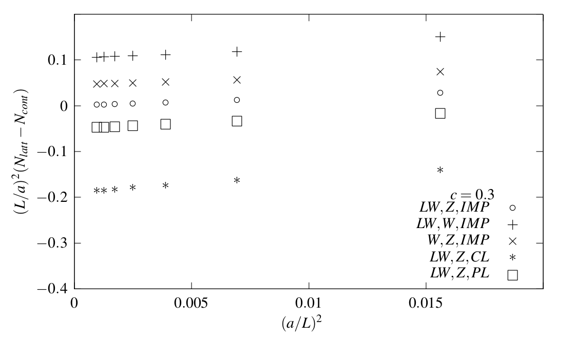
Figure 1: The figure shows O($a^{2}$) cutoff effects with SF boundary conditions at $c=0.3$. The labels are ordered in such a way they indicate action, flow, and observable. $O(a^{2})$ improvement is seen only with LW action, Zeuthen flow and improved observable. We then ”unimprove” one by one to distinguish the cutoff effects origination from the Wilson action, Wilson flow and plaquette/clover observables, respectively.

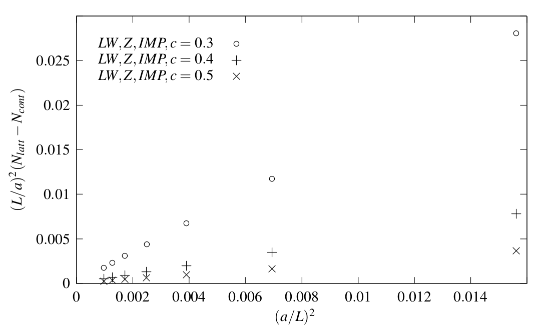
Figure 2: O($a^{2}$) improved data for $c=0.3,0.4,0.5$ and with SF boundary conditions, cf. text.

5 Conclusion

We confirm expectations based on the O($a^{2}$) improved framework of ref. [5] and previous results in [7]. We have derived a convenient representation of the gauge field propagator using the set-up proposed in [8], which allows us to apply an orbifold reflection principle. We anticipate that the gauge propagator representation will be very useful in future perturbative computations which might be needed to complement a non-diagrammatic numerical approach [12, 13].

References

• [1] M.ย Lรผscher, JHEP 1008 (2010) 071 Erratum: [JHEP 1403 (2014) 092] [arXiv:1006.4518 [hep-lat]].
• [2] M.ย Lรผscher and P.ย Weisz, JHEP 1102 (2011) 051 [arXiv:1101.0963 [hep-th]].
• [3] M.ย Lรผscher, PoS LATTICE 2013 (2014) 016 [arXiv:1308.5598 [hep-lat]].
• [4] A.ย Ramos, PoS LATTICE 2014 (2015) 017 [arXiv:1506.00118 [hep-lat]].
• [5] A.ย Ramos and S.ย Sint, Eur.ย Phys.ย J.ย C 76 (2016) no.1, 15 [arXiv:1508.05552 [hep-lat]].
• [6] P.ย Fritzsch and A.ย Ramos, JHEP 1310 (2013) 008 doi:10.1007/JHEP10(2013)008 [arXiv:1301.4388 [hep-lat]].
• [7] M.ย Dalla Brida et al. [ALPHA Collaboration], arXiv:1607.06423 [hep-lat].
• [8] M.ย Lรผscher, JHEP 1406 (2014) 105 [arXiv:1404.5930 [hep-lat]].
• [9] Y.ย Taniguchi, JHEP 0512 (2005) 037 [hep-lat/0412024].
• [10] S.ย Sint, Nucl.ย Phys.ย B 847 (2011) 491 [arXiv:1008.4857 [hep-lat]].
• [11] C.ย Sanderson and R.ย Curtin, Journal of Open Source Software, 1, 26 (2016).
• [12] M.ย Dalla Brida and D.ย Hesse, PoS Lattice 2013 (2014) 326 [arXiv:1311.3936 [hep-lat]].
• [13] M.ย Dalla Brida and M.ย Lรผscher, arXiv:1612.04955 [hep-lat], PoS Lattice 2016 332 (to appear).