Loschmidt Echo Revivals: Critical and Noncritical
Abstract
A quantum phase transition is generally thought to imprint distinctive characteristics on the nonequilibrium dynamics of a closed quantum system. Specifically, the Loschmidt echo after a sudden quench to a quantum critical point measuring the time dependence of the overlap between initial and time-evolved states is expected to exhibit an accelerated relaxation followed by periodic revivals. We here introduce a new exactly solvable model, the extended Su-Schrieffer-Heeger model, the Loschmidt echo of which provides a counterexample. A parallell analysis of the quench dynamics of the three-site spin-interacting model allows us to pinpoint the conditions under which a periodic Loschmidt revival actually appears.
pacs:
03.65.Yz, 05.30.-d, 64.70.TgTaking a quantum system out of equilibrium can be done in many ways, such as injecting energy through an external reservoir or applying a driving field. The simplest paradigm is maybe that of a quantum quench, where a closed system is pushed out of equilibrium by a sudden change in the Hamiltonian which controls its time evolution. Studies of quantum quenches have spawned a large body of results, on equilibration and thermalization Gogolin and Eisert (2016) (and its breakdown in integrable systems Vidmar and Rigol (2016)), on entanglement dynamics Calabrese and Cardy (2016), and more Polkovnikov et al. (2011); Mitra (2017). In this context, an important task is to identify nonequilibrium dynamical signatures of a quantum phase transition (QPT). The problem comes in a variety of shapes, ranging from the Kibble-Zurek mechanism for defect production Zurek et al. (2005) to the time evolution of correlations in strongly correlated out-of-equilibrium systems at a QPT Manmana et al. (2007). A basic variant is to ask the question: If a Hamiltonian is suddenly quenched to a quantum critical point (or its vicinity), is there any special characteristic of the subsequent dynamics?
To address this question one may invoke the Loschmidt echo (LE) Gorin et al. (2006), which measures the overlap between the initial (prequench) and time-evolved (postquench) state. Applied to a quantum critical quench i.e. with the quench parameter pulled to a quantum critical point finite-size case studies reveal that the time dependence of the LE of several models exhibits a periodic pattern, a revival structure, formed by brief detachments from its mean value Quan et al. (2006); Yuan et al. (2007); Rossini et al. (2007a); Zhong and Tong (2011); Häppölä et al. (2012); Montes and Hamma (2012); Sharma et al. (2012); Rajak and Divakaran (2014), implying revivals also for expectation values of local observables Iglói and Rieger (2011); Cardy (2014). The amplitudes of these revivals may decay with time, however, their presence appears to be independent of the initial state and the size of the quench Häppölä et al. (2012). Indeed, the distinctive structure of revivals of the LE after a quench has been conjectured to be a faithful witness of quantum criticality Quan et al. (2006); Yuan et al. (2007).
In this Letter we challenge the notion that quantum criticality and LE revival structures are intrinsically linked. We do this by way of example, introducing a new exactly solvable model, the extended Su-Schrieffer-Heeger (ESSH) model, which exhibits several distinct quantum phases with associated QPTs. The ESSH model serves as a representative of a large class of quasifree 1D Fermi systems, and contains as special cases the original SSH model Su et al. (1979), the Creutz model Creutz (1999), and the Kitaev chain Kitaev (2001) and its dimerized version Wakatsuki et al. (2014). Moreover, via a Jordan-Wigner transformation Lieb et al. (1961), and with suitably chosen parameters, the ESSH model embodies several generic spin chain models, including the 1D quantum compass model Nussinov and van den Brink (2015). Important for the present work, the quench dynamics of the ESSH model highlights the conditions under which the LE may show a revival structure. Informed by this, and by results extracted from another exactly solvable model, the three-site spin-interacting (TSSI) model Titvinidze and Japaridze (2003); Zvyagin and Skorobagat’ko (2006), we come to the conclusion that quantum criticality is neither a sufficient nor a necessary condition for the LE to exhibit an observable revival structure. Instead, what matters is that the quasiparticle modes which control the LE are massless and have a group velocity , where is the length of the system and is the observation time. Only if these modes coincide with the quantum critical modes is a revival structure tied to a QPT. These conditions, which are general, bring new light on the important issue of how to read a LE after a quantum quench.
Loschmidt echo. A quantum quench is a sudden change in the Hamiltonian of a quantum system, with denoting the value(s) of the parameter(s) that will be quenched. The system is initially prepared in an eigenstate to the Hamiltonian . The quench is carried out at time , when is suddenly switched to . The system then evolves with the quench Hamiltonian according to . In this case the LE Gorin et al. (2006), here denoted by , reduces to a dynamical version of the ground-state fidelity (return probability),
| (1) |
measuring the distance between the time-evolved state and the initial state .
The LE typically decays in a short time (relaxation time), from unity to some mean value around which it then fluctuates Venuti et al. (2011). Revivals are also visible in the LE as pronounced deviations from the average value Häppölä et al. (2012). For quenches to a quantum critical point in a finite system there is an expectation that the LE relaxation is accelerated Quan et al. (2006); Yuan et al. (2007); Zhang et al. (2009); Rossini et al. (2007a, b); Sharma et al. (2012); Sacramento. (2016) and that the revivals are periodic Quan et al. (2006); Yuan et al. (2007); Häppölä et al. (2012); Montes and Hamma (2012). Conversely, such behavior has been proposed as a signature of quantum criticality Quan et al. (2006); Yuan et al. (2007). However, the matter turns out to be more complex. To see how, we next introduce the ESSH model and exhibit its quench dynamics.
Extended Su-Schrieffer-Heeger (ESSH) model.
We define the Hamiltonian of the ESSH model by
where and are sublattice indices labeling fermion creation and annihilation operators and , and are hopping amplitudes, and are superconducting pairing gaps, are the phases of the pairing terms, and is a chemical potential. Choosing and introducing the Nambu spinor , the Fourier transformed Hamiltonian can be expressed in Bogoliubov-de Gennes (BdG) form Zhu (2016), , with
| (7) |
where and . Here , , given periodic boundary conditions, and with the lattice spacing, taken as unity in arbitrary units.
By diagonalizing one obtains the quasiparticle Hamiltonian , with and linear combinations of the elements in the Nambu spinor, and with corresponding energy bands and , where and . The ground state is obtained by filling up the negative-energy quasiparticle states, , where is the Bogoliubov vacuum annihilated by the ’s (see Supplemental Material Jafari and Johannesson (2016)).
One easily verifies that the gap to the first excited state vanishes for all momenta when , , and . The ground state here acquires a degeneracy of (enlarged to at the isotropic point (IP) ) Jafari and Johannesson (2016). It follows that the line in parameter space is critical for any ratio . Its interpretation is most easily phrased in spin language by connecting the ESSH model to the general quantum compass model You et al. (2014); Nussinov and van den Brink (2015) via a Jordan-Wigner transformation Lieb et al. (1961). The critical line is then seen to define a (nontopological) QPT between two distinct phases with large short-range spin correlations in the and direction respectively. As expected Zanardi et al. (2007), this QPT is signaled by a sharp decay of the ground-state fidelity , cf. Fig. S2 in Jafari and Johannesson (2016).
Loschmidt echo in the ESSH model. By a rather lengthy calculation one can obtain the complete set of eigenstates of the model, yielding an exact expression for the LE Jafari and Johannesson (2016) When the system is initialized in the ground state and quenched to the critical line, i.e. with , one obtains
| (8) |
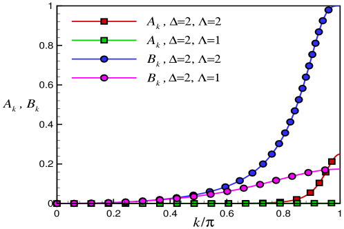
where and measure overlaps between modes of the initial ground state, , and eigenstates of ; cf. Fig. 1 and Jafari and Johannesson (2016). The energies are those of the quasiparticles in the lowest filled band in the ground state of the critical quench Hamiltonian.
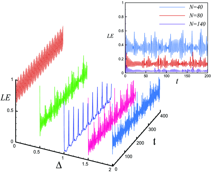
In Fig. 2 we have plotted versus and time for quenches to the critical line starting from , for , and . One clearly sees a rapid decay of the LE, with periodic revivals in time when quenching to the IP . This is in agreement with several studies of LEs at quantum criticality Quan et al. (2006); Yuan et al. (2007); Venuti et al. (2011); Häppölä et al. (2012); Montes and Hamma (2012); Zhang et al. (2009); Haikka et al. (2012); Rajak and Divakaran (2014); Rossini et al. (2007a, b); Sharma et al. (2012); Zhong and Tong (2011). However, departing from the IP, taking , but remaining at the critical line , a surprising result occurs: The periodic revivals get wiped out for sufficiently large anisotropies, with the LE oscillating randomly around its mean value.
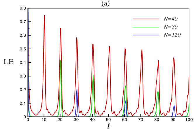
To find out why the LE exhibits a revival structure at or very close to the IP, but not farther away from the IP, let us begin by pinpointing the revival periods at the IP, manifest in Fig. 3(a). Plotting versus , cf. Fig. 3(b), unveils a linear scaling
| (9) |
where has dimension of velocity with value . A numerical spectral analysis suggests that , where , cf. inset, Fig. 3(b). This result is anticipated from a study of the spin-1/2 model Häppölä et al. (2012), where the LE revival period is also governed by the maximum quasiparticle group velocity produced by the critical quench Hamiltonian. However, Eq. (9), with , fails to account for the disappearance of periodic revivals away from the IP. Why is that?
The answer lies in Eq. (8). First note that a revival requires that all modes in Eq. (8) contribute sizably to the LE, in turn requiring that the oscillating terms are small. An analysis shows that the oscillation amplitudes and are indeed small except for when approaching the BZ boundary (at which takes its maximum), cf. Fig. 1. It follows that the corresponding modes can contribute constructively to the LE only at time instances at which their oscillation terms get suppressed. Thus, we expect that the most pronounced revivals happen when the vanishing of the term proportional to is concurrent with the near vanishing of terms with close to . To obtain the revival period at the IP we thus make the ansatz , with an integer and with the mode with the largest group velocity in the vicinity of the BZ boundary. A Taylor expansion to first order, shows that terms of neighboring modes are strongly suppressed whenever is a multiple of with and (as before) . Here are integers and . This estimate of the revival period agrees with the numerical result in Eq. (9).
Turning to the anisotropic case and repeating the analysis from above immediately reveals why the revival structure now gets lost. First, as exemplified in Fig. 1, the amplitudes are here small for all modes. Thus, the simultaneous suppression of the dominant (but still small) oscillation terms is not expected to have a significant effect on the LE. Moreover, as seen in the inset of Fig. 3(b), the group velocities away from the IP are quite small throughout the range where is nonvanishing. As a consequence, with (as before obtained by expanding the quasiparticle energies close to where the amplitudes are largest), one would have to wait an exceedingly long time to see any trace of a weak revival structure, if at all present.
To understand the origin of the different behaviors of the LE at the IP and away from the IP, recall from Eq. (8) that the revivals are controlled by quasiparticles in the lowest energy band, . This is so since the second filled quasiparticle band in the ground state, , collapses to zero and becomes dispersionless at the critical line Jafari and Johannesson (2016). Away from the IP, the band remains gapped for all also at the critical line, thus holding back quasiparticle excitations from that band. This is different from the critical line at the IP where the gap closes at the BZ boundary Jafari and Johannesson (2016). Since the oscillation amplitudes can be interpreted as measuring the probabilities of quasiparticle excitations, modes at or near the gap-closing points are indeed expected to yield much larger amplitudes. As follows from our result for the revival period, if these modes also give rise to a group velocity , with the observation time, a revival structure will ensue. Note that here is the group velocity of quasiparticles at which the oscillation amplitudes peak. While happens to be at a global maximum in the ESSH model at the IP, this property is not expected to be generic.
Loschmidt echo in the three-site spin-interacting model. Having established that quantum criticality is not a sufficient condition for a revival structure in a LE, what about the converse? Can a LE exhibit a revival structure without the presence of a QPT?
The answer is yes. A case in point is the LE of a quench to the line in the - parameter space of the three-site spin-interacting (TSSI) XY model Titvinidze and Japaridze (2003); Zvyagin and Skorobagat’ko (2006),
| (10) | |||||
where , and are the usual Pauli matrices. In Ref. Divakaran (2013) it was noted that the decay rate of the LE shows an accelerated decay in such a quench, independent of whether the quench is critical () or noncritical (). In contrast, the LEs of quenches to the critical lines which define a QPT between an antiferromagnetic and type-I spin-liquid phase display neither enhanced decays nor revival structures.
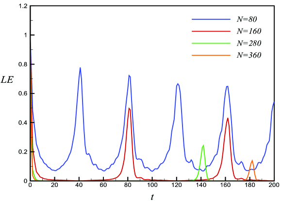
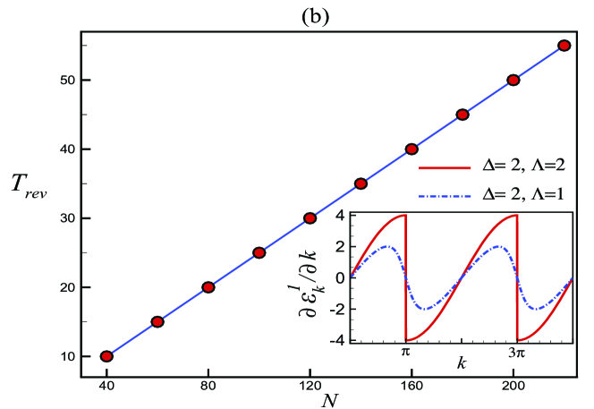
Guided by our results for the ESSH model, we resolve this conundrum by numerically confirming that the absence of a revival structure for a quench from the antiferromagnetic phase to the critical lines of the TSSI XY model is linked to consistently small oscillation amplitudes in the mode decomposition of the LE. Analogous to the ESSH model away from the IP, this can be attributed to the fact that the quasiparticles which control the LE remain fully gapped as one approaches the QPT. On the contrary, the revival structures which do appear in the TSSI LEs are associated with large oscillation terms in the mode decomposition of the LE, with amplitudes that peak at wave numbers where nearby quasiparticles have a sizable group velocity. This, in turn, emulates the scenario for the ESSH model at the IP, but now for quenches to special parameter values which do not define a critical point of a QPT. One should here note that while a QPT may favor large LE oscillation amplitudes Venuti and Zanardi (2010) (however as transpires from our analysis only if these are controlled by the quasiparticles which become massless at the QPT), large amplitudes can incidentally appear also within a quantum phase if this phase supports massless excitations. Provided that these excitations have sizable group velocities, an observable revival structure may then emerge, as evidenced when quenching to the noncritical line within the type-I spin-liquid phase of the TSSI XY model, cf. Fig. 4.
Summary. We have shown that the presence of a quantum phase transition is neither a sufficient nor a necessary condition for observing a revival structure in the Loschmidt echo after a quantum quench. Periodic revivals are preconditioned by a LE controlled by massless quasiparticle modes with a group velocity , where is the length of the system and is the observation time. This property may or may not be present at a quantum critical point. The suppression of a critical revival structure is strikingly illustrated away from the isotropic quantum critical point in the extended Su-Schrieffer-Heeger model, introduced in this Letter. Here the revivals are found to be controlled by quasiparticle states which remain gapped at the anisotropic quantum phase transition, implying small oscillation amplitudes in the mode decomposition of the LE. Our findings may call for a revisit of earlier results on revival structures and quantum criticality, and should encourage efforts to identify more reliable nonequilibrium markers of quantum criticality.
Acknowledgements.
Acknowledgments H. J. thanks Wen-Long You for valuable discussions. R. Jafari would like to dedicate this paper to Prof. Y. Sobouti the founder of Institute for Advanced Studies in Basic Sciences. This research was supported by STINT (Grant No. IG2011-2028) and the Swedish Research Council (Grant No. 621-2014-5972).References
- Gogolin and Eisert (2016) C. Gogolin and J. Eisert, Rep. Prog. Phys. 79, 056001 (2016).
- Vidmar and Rigol (2016) L. Vidmar and M. Rigol, J. Stat. Mech.: Theor. Exp. P064007 (2016).
- Calabrese and Cardy (2016) P. Calabrese and J. Cardy, J. Stat. Mech.: Theor. Exp. P064003 (2016).
- Polkovnikov et al. (2011) A. Polkovnikov, K. Sengupta, A. Silva, and M. Vengalattore, Rev. Mod. Phys. 83, 863 (2011).
- Mitra (2017) A. Mitra, Annu. Rev. Condens. Matter Phys. 8 (2017).
- Zurek et al. (2005) W. H. Zurek, U. Dorner, and P. Zoller, Phys. Rev. Lett. 95, 105701 (2005).
- Manmana et al. (2007) S. R. Manmana, S. Wessel, R. M. Noack, and A. Muramatsu, Phys. Rev. Lett. 98, 210405 (2007).
- Gorin et al. (2006) T. Gorin, T. Prosen, T. H. Seligman, and M. Znidaric, Phys. Rep. 435, 33 (2006).
- Quan et al. (2006) H. T. Quan, Z. Song, X. F. Liu, P. Zanardi, and C. P. Sun, Phys. Rev. Lett. 96, 140604 (2006).
- Yuan et al. (2007) Z.-G. Yuan, P. Zhang, and S.-S. Li, Phys. Rev. A 75, 012102 (2007).
- Rossini et al. (2007a) D. Rossini, T. Calarco, V. Giovannetti, S. Montangero, and R. Fazio, Phys. Rev. A 75, 032333 (2007a).
- Zhong and Tong (2011) M. Zhong and P. Tong, Phys. Rev. A 84, 052105 (2011).
- Häppölä et al. (2012) J. Häppölä, G. B. Halász, and A. Hamma, Phys. Rev. A 85, 032114 (2012).
- Montes and Hamma (2012) S. Montes and A. Hamma, Phys. Rev. E 86, 021101 (2012).
- Sharma et al. (2012) S. Sharma, V. Mukherjee, and A. Dutta, Eur. Phys. J. B 85, 143 (2012).
- Rajak and Divakaran (2014) A. Rajak and U. Divakaran, J. Stat. Mech.: Theor. Exp. P04023 (2014).
- Iglói and Rieger (2011) F. Iglói and H. Rieger, Phys. Rev. Lett. 106, 035701 (2011).
- Cardy (2014) J. Cardy, Phys. Rev. Lett. 112, 220401 (2014).
- Su et al. (1979) W. P. Su, J. R. Schrieffer, and A. J. Heeger, Phys. Rev. Lett. 42, 1698 (1979).
- Creutz (1999) M. Creutz, Phys. Rev. Lett. 83, 2636 (1999).
- Kitaev (2001) A. Y. Kitaev, Phys. Usp. 44, 131 (2001).
- Wakatsuki et al. (2014) R. Wakatsuki, M. Ezawa, Y. Tanaka, and N. Nagaosa, Phys. Rev. B 90, 014505 (2014).
- Lieb et al. (1961) E. Lieb, T. Schultz, and D. Mattis, Ann. Phys. 16, 407 (1961).
- Nussinov and van den Brink (2015) Z. Nussinov and J. van den Brink, Rev. Mod. Phys. 87, 1 (2015).
- Titvinidze and Japaridze (2003) I. Titvinidze and G. I. Japaridze, Eur. Phys. J. B 32, 383 (2003).
- Zvyagin and Skorobagat’ko (2006) A. A. Zvyagin and G. A. Skorobagat’ko, Phys. Rev. B 73, 024427 (2006).
- Venuti et al. (2011) L. Campos Venuti, N. T. Jacobson, S. Santra, and P. Zanardi, Phys. Rev. Lett. 107, 010403 (2011).
- Zhang et al. (2009) J. Zhang, F. M. Cucchietti, C. M. Chandrashekar, M. Laforest, C. A. Ryan, M. Ditty, A. Hubbard, J. K. Gamble, and R. Laflamme, Phys. Rev. A 79, 012305 (2009).
- Rossini et al. (2007b) D. Rossini, T. Calarco, V. Giovannetti, S. Montangero, and R. Fazio, J. Phys. A.: Math. Theor. 40, 8033 (2007b).
- Sacramento. (2016) P. D. Sacramento, Phys. Rev. E 93, 062117 (2016).
- Zhu (2016) J.-X. Zhu, Bogoliubov-de Gennes Method and Its Applications (Springer, Berlin and New York, 2016).
- Jafari and Johannesson (2016) R. Jafari and H. Johannesson, Supplemental Material (2016).
- You et al. (2014) W.-L. You, P. Horsch, and A. M. Oleś, Phys. Rev. B 89, 104425 (2014).
- Zanardi et al. (2007) P. Zanardi, P. Giorda, and M. Cozzini, Phys. Rev. Lett. 99, 100603 (2007).
- Haikka et al. (2012) P. Haikka, J. Goold, S. McEndoo, F. Plastina, and S. Maniscalco, Phys. Rev. A 85, 060101 (2012).
- Divakaran (2013) U. Divakaran, Phys. Rev. E 88, 052122 (2013).
- Venuti and Zanardi (2010) L. Campos Venuti and P. Zanardi, Phys. Rev. A 81, 022113 (2010).
I Supplementary material
In this Supplemental Material we have collected some useful results on the extended Su-Schrieffer-Heeger (ESSH) model, introduced in the accompanying Letter, Ref. Jafari and Johannesson (2016).
I.1 A. Eigenstates and eigenvalues of the ESSH model
By Fourier transforming the ESSH Hamiltonian in Eq. (2) in Jafari and Johannesson (2016), choosing , and grouping together terms with and , is transformed into a sum of commuting Hamiltonians , each describing a different mode,
| (S1) |
Here and , with the lattice spacing. We can thus obtain the spectrum of the ESSH model by diagonalizing each Hamiltonian mode in (S1) independently. This can be done in two ways: Using a generalized Bogoliubov transformation which maps onto the BdG quasiparticle Hamiltonian in (3) in Jafari and Johannesson (2016) (with the quasiparticle operators and , expressed in terms of the fermion operators in (S1)), or using a basis in which the eigenstates of are obtained as linear combinations of even-parity fermion states Sun and Chen (2009). Here we outline the connection between the two approaches.
As in (S1) conserves the number parity (even or odd number of fermions), it is sufficient to consider the even-parity subspace of the Hilbert space. This subspace is spanned by the eight basis vectors
| (S2) |
The eigenstates of in this basis can be written as
| (S3) |
where is an unnormalized eigenstate of with corresponding eigenvalue , and where are functions of the amplitudes of the hopping () and pairing terms (), the pairing phases , and the momentum . Four eigenstates are degenerate with eigenvalues zero (), with the ground state and the first excited state having negative energies ( respectively). Here and are the quasiparticle energies defined after Eq. (3) in Jafari and Johannesson (2016).
Each eigenstate of can be linked to a state in the BdG formalism via their common eigenvalues. For instance, the ground state of is identified with the BdG mode with the corresponding negative energy quasiparticle states filled, i.e. , where is the single-fermion mode of the Bogoliubov vacuum. Since the connection between quasiparticle operators and fermion operators is fixed by the Bogoliubov transformation, we can calculate the Bogoliubov vacuum in terms of the eigenstates of :
| (S4) |
where are functions of the parameters , and , and the momentum . The resulting explicit expression is rather unwieldy. Let us point out that while the BdG formalism is very convenient for obtaining energy eigenvalues, the fermionic even-parity basis is preferable for numerically computing matrix elements of the time-evolved states, such as those which enter the Loschmidt echo.
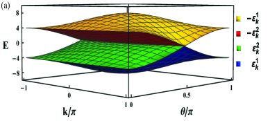
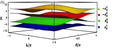
I.2 B. Quasiparticle spectrum
The BdG quasiparticle spectrum of the ESSH model is plotted in Fig. S1 at (a) the isotropic point (IP) and (b) at the anisotropic point . The many-particle groundstate of the ESSH Hamiltonian for is obtained by filling the two lowest bands, and . As seen, at the IP the energy gap between the and bands closes at (Fig. S1(a)) while it is nonzero away from the IP (Fig. S1(b)). In contrast, and as required for the existence of the quantum critical line , the energy gap between the and bands is closed for all momenta at for arbitrary values of . One verifies that the groundstate has a -fold degeneracy at the critical line off the IP, with an enlarged degeneracy right at the IP.
I.3 C. Loschmidt echo
The mode decomposition of the Loschmidt echo in the ESSH model takes the form
| (S5) | |||||
| (S6) | |||||
where is the normalization factor of the eigenstate , and where are functions of the parameters and in the ESSH Hamiltonian, Eq. (2) in Jafari and Johannesson (2016). For a quench to the critical line , the LE reduces to the simple form
| (S7) |
where is the ground state energy of at the critical line. Furthermore, and , where . The oscillation amplitudes and are plotted versus in Fig. 1 in Jafari and Johannesson (2016), at the IP and away from the IP. As seen in the figure, the -amplitudes at the IP for approaching the BZ boundary are significantly larger than those away from the IP.
I.4 D. Fidelity
By considering the ground state of the system as the initial state, the LE can be interpreted as a dynamical version of the squared ground-state fidelity , defined by the overlap between two ground states at different parameter values and : . The ground-state fidelity of the ESSH model can be decomposed as
| (S8) |
| (S9) |
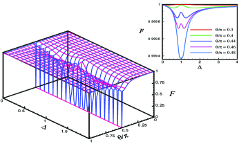
with functions of the parameters in the ESSH Hamiltonian, Eq. (2) in Jafari and Johannesson (2016). A ground-state fidelity serves as a marker of QPTs Zanardi et al. (2007), with the QPT at the ESSH critical line signaled by a sharp decay of , see Fig. S2. Intriguingly, as seen in the inset of this figure, the fidelity develops extrema away from the critical line , with a local maximum unfolding as one approaches the isotropic point (IP) . We conjecture that this reflects the enhanced groundstate degeneracy at the IP; cf. Sec. B above.
I.5 E. Symmetries and topological phases
The ESSH Hamiltonian in Eq. (2) in Jafari and Johannesson (2016) has particle-hole symmetry, but not time-reversal or chiral symmetry.
To verify this, first note that a particle-hole transformation in the Nambu spinor basis, defined after Eq. (2) in Jafari and Johannesson (2016), is carried out by the operator , where is complex conjugation and . One easily checks that where is the BdG Hamiltonian in Eq. (3) in Jafari and Johannesson (2016). Turning to the time-reversal operator , it is given simply by since the fermions in the ESSH model are spinless. Inspection of immediately reveals that time-reversal symmetry is broken. The chiral symmetry operator can by expressed as , and one checks that this symmetry is also broken. The presence of sublattice symmetry, , with does not alleviate this fact since in the Nambu spinor basis chiral symmetry does not originate in a lattice substructure. It follows that the model is in the D symmetry class with a topological index Schnyder et al. (2008) .
The index is nonzero in the topologically nontrivial phases of the model. These phases can appear when letting the Hamiltonian parameters take values and (not considered in Jafari and Johannesson (2016)). For example, for , the system is in the Kitaev-like Kitaev (2001); Wakatsuki et al. (2014) topological phase for . By increasing the pairing phase , the system enters the SSH-like trivial phase Wang and Zhang (2012) at in which the index is zero. The system once again goes into a Kitaev-like topological phase for . The revival period of the Loschmidt echo after a quench to the topological phase transition points and is governed by Eq. (5) in Jafari and Johannesson (2016), with the group velocity of the critical modes Jafari and Johannesson (2017).
I.6 F. Connection to the general quantum compass model
The Hamiltonian of the 1D spin- general quantum compass model is given by You et al. (2014)
| (S10) |
with exchange amplitudes on even/odd lattice bonds, and where the pseudo-spin operators are formed by linear combinations of the Pauli matrices and : . This Hamiltonian can be diagonalized exactly by mapping it onto a free fermion model,
| (S11) |
using the Jordan-Wigner transformation
| (S12) |
By partitioning the chain into bi-atomic elementary cells and defining two independent fermions at each cell Perk et al. (1975); Derzhko et al. (2009), and , one can rewrite the Hamiltonian in Eq. (S10) as
| (S13) |
Choosing the parameters of the ESSH Hamiltonian, Eq. (2) in Jafari and Johannesson (2016), as , , and , it maps onto the Hamiltonian in Eq. (S13).
In other words, the ESSH model in this case represents the general quantum compass model.
References
- Jafari and Johannesson (2016) R. Jafari and H. Johannesson, accompanying Letter (2016).
- Sun and Chen (2009) K.-W. Sun and Q.-H. Chen, Phys. Rev. B 80, 174417 (2009).
- Zanardi et al. (2007) P. Zanardi, P. Giorda, and M. Cozzini, Phys. Rev. Lett. 99, 100603 (2007).
- Schnyder et al. (2008) A. P. Schnyder, S. Ryu, A. Furusaki, and A. W. W. Ludwig, Phys. Rev. B 78, 195125 (2008).
- Kitaev (2001) A. Y. Kitaev, Physics Uspekhi 44, 131 (2001).
- Wakatsuki et al. (2014) R. Wakatsuki, M. Ezawa, Y. Tanaka, and N. Nagaosa, Phys. Rev. B 90, 014505 (2014).
- Wang and Zhang (2012) Z. Wang and S.-C. Zhang, Phys. Rev. X 2, 031008 (2012).
- Jafari and Johannesson (2017) R. Jafari and H. Johannesson, unpublished (2017).
- You et al. (2014) W.-L. You, P. Horsch, and A. M. Oleś, Phys. Rev. B 89, 104425 (2014).
- Perk et al. (1975) J. Perk, H. Capel, M. Zuilhof, and T. Siskens, Physica A 81, 319 (1975), ISSN 0378-4371.
- Derzhko et al. (2009) O. Derzhko, T. Krokhmalskii, J. Stolze, and T. Verkholyak, Phys. Rev. B 79, 094410 (2009).