Temporal correlations between the earthquake magnitudes before major mainshocks in Japan

Abstract

A characteristic change of seismicity has been recently uncovered when the precursory Seismic Electric Signals activities initiate before an earthquake occurrence. In particular, the fluctuations of the order parameter of seismicity exhibit a simultaneous distinct minimum upon analyzing the seismic catalogue in a new time domain termed natural time and employing a sliding natural time window comprising a number of events that would occur in a few months. Here, we focus on the minima preceding all earthquakes of magnitude 8 (and 9) class that occurred in Japanese area from 1 January 1984 to 11 March 2011 (the day of the M9 Tohoku earthquake). By applying Detrended Fluctuation Analysis to the earthquake magnitude time series, we find that each of these minima is preceded as well as followed by characteristic changes of temporal correlations between earthquake magnitudes. In particular, we identify the following three main features. The minima are observed during periods when long range correlations have been developed, but they are preceded by a stage in which an evident anti-correlated behavior appears. After the minima, the long range correlations break down to an almost random behavior turning to anti-correlation. The minima that precede M$\geq$7.8 earthquakes are distinguished from other minima which are either non-precursory or followed by smaller earthquakes.

I Introduction

Seismic Electric Signals (SES) are low frequency ($\leq 1$Hz) transient changes of the electric field of the Earth that have been found (Varotsos and Alexopoulos, 1984; Varotsos et al., 1996) to precede earthquakes (EQs). Several such transient changes within a short time are termed SES activity. A model for the SES generation has been proposed (Varotsos and Alexopoulos, 1986) (see also Varotsos et al. (1993)) based on the widely accepted concept that the stress gradually increases in the future focal region of an EQ. It was postulated that when this stress reaches a critical value, a cooperative orientation of the electric dipoles (which anyhow exist in the focal area due to lattice defects in the ionic constituents of the rocks) occurs, which leads to the emission of a transient electric signal. All solids including metals, insulators and semiconductors contain intrinsic and extrinsic defects(Varotsos and Miliotis, 1974; Kostopoulos et al., 1975; Varotsos and Alexopoulos, 1977, 1980, 1978; Varotsos, 1980; Varotsos and Alexopoulos, 1982; Varotsos et al., 1982; Varotsos, 2008). The model is consistent with the finding that the time series of the observed SES activities (along with their associated magnetic field variations) exhibit infinitely ranged temporal correlations (Varotsos et al., 2003a, b; Varotsos et al., 2008, 2009), thus being in accord with the conjecture of critical dynamics. Other possible mechanisms for SES generation such as the recently developed finite fault rupture model with the electrokinetic effect(Ren et al., 2012) and the piezoelectric effect(Varotsos, 1978) taking into account the fault dislocation theory(Huang, 2011) have been proposed, see also Ch. 1 of Varotsos et al. (2011a). The observations of SES activities in Greece (Varotsos and Lazaridou, 1991; Varotsos et al., 1993; Varotsos et al., 2011a) have shown that their lead time is of the order of a few months. This agrees with later observations in Japan (Uyeda et al., 2000, 2002, 2009; Orihara et al., 2012).

EQs may be considered as (non-equilibrium) critical phenomena since the observed EQ scaling laws (Turcotte, 1997) point to the existence of phenomena closely associated with the proximity of the system to a critical point (Holliday et al., 2006). An order parameter for seismicity has been introduced (Varotsos et al., 2005) in the frame of the analysis in a new time domain termed natural time $\chi$ (see below). This analysis has been found to reveal novel dynamical features hidden in the time series of complex systems (Varotsos et al., 2011a).

A unique change of the order parameter of seismicity approximately at the time when SES activities initiate has been recently uncovered (Varotsos et al., 2013). In particular, upon analyzing the Japanese seismic catalogue in natural time, and employing a sliding natural time window comprising the number of events that would occur in a few months, the following was observed: The fluctuations of the order parameter of seismicity exhibit a clearly detectable minimum approximately at the time of the initiation of the pronounced SES activity observed by Uyeda et al. (2002, 2009) almost two months before the onset of the volcanic-seismic swarm activity in 2000 in the Izu Island region, Japan. (This swarm was then characterized by Japan Meteorological Agency (JMA) as being the largest EQ swarm ever recorded Japan Meteorological Agency (2000).) This reflects that presumably the same physical cause led to both effects, i.e, the emission of the SES activity and the change of the correlation properties between the EQs. In addition, these two phenomena were found (Varotsos et al., 2013) to be also linked in space.

For the vast majority of major EQs in Japan, however, the aforementioned almost simultaneous appearance of the minima of the fluctuations of the order parameter of seismicity with the initiation of SES activities, cannot be directly verified due to the lack of geolectrical data. In view of this lack of data, an investigation was made (Sarlis et al., 2013) that was solely focused on the question whether minima of the fluctuations of seismicity are observed before all EQs of magnitude 7.6 or larger that occurred from 1 January 1984 to 11 March 2011 (the day of the M9 Tohoku EQ) in Japanese area. Actually such minima were identified a few months before these EQs. It is the main scope of this paper to investigate the temporal correlations between the EQ magnitudes by paying attention to the time periods during which the minima of the order parameter fluctuations of seismicity have been observed before EQs of magnitude 8 (and 9) class (cf. Sarlis et al. (2013) also studied the M7.6 Far-Off Sanriku EQ which however is not studied in detail here -but only shortly commented in the last paragraph of the Appendix- since it belongs to a smaller magnitude class, i.e., the 7-7.5 class, being a single asperity event(Yamanaka and Kikuchi, 2004)). Their epicenters are shown in Fig. 1 (see also Table 1). Along these lines, we employ here the Detrended Fluctuation Analysis (DFA) (Peng et al., 1994) which has been established as a standard method to investigate long range correlations in non-stationary time series in diverse fields (e.g., Peng et al. (1993, 1994, 1995); Ashkenazy et al. (2002); Ivanov et al. (2009); Ivanov (2007); Talkner and Weber (2000); Goldberger et al. (2002); Telesca and Lovallo (2009); Telesca and Lasaponara (2006); Telesca et al. (2012)) including the study of geomagnetic data associated with the M9.0 Tohoku EQ (Rong et al., 2012). For example, a recent study (Shao et al., 2012) showed that DFA as well as the Centered Detrended Moving Average technique remain “The Methods of Choice” in determining the Hurst index of time series. As we shall see, the results of DFA obtained here in conjunction with the aforementioned minima emerged from natural time analysis lead to conclusions that are of key importance for EQ prediction research. In particular, we find that each of these precursory minima of the fluctuations of the order parameter of seismicity is preceded as well as followed by characteristic changes of temporal correlations between EQ magnitudes, thus complementing the results of Sarlis et al. (2013).

II The procedure followed in the analysis

In a time series comprising $N$ consecutive events, the natural time of the $k$-th event of energy $Q_{k}$ is defined by $\chi_{k}=k/N$ (Varotsos et al., 2001; Varotsos et al., 2002a, b). We then study the evolution of the pair $(\chi_{k},p_{k})$, where $p_{k}={Q_{k}}/{\sum_{n=1}^{N}Q_{n}}$ is the normalized energy. This analysis, termed natural time analysis, extracts from a given complex time series the maximum information possible (Abe et al., 2005). The approach of a dynamical system to a critical point can be identified (Varotsos et al., 2001; Varotsos et al., 2011a, b) by means of the variance $\kappa_{1}$ of natural time $\chi$ weighted for $p_{k}$, namely

$$\kappa_{1}=\sum_{k=1}^{N}p_{k}(\chi_{k})^{2}-\left(\sum_{k=1}^{N}p_{k}\chi_{k}\right)^{2}\equiv\langle\chi^{2}\rangle-\langle\chi\rangle^{2}$$ (1)

It has been argued(Varotsos et al., 2005) (see also pp. 249-253 of Varotsos et al. (2011a)) that the quantity $\kappa_{1}$ of seismicity can serve as an order parameter. To compute the fluctuations of $\kappa_{1}$ we apply the following procedure (Varotsos et al., 2011a; Sarlis et al., 2013): First, take an excerpt comprising $W(\geq 100)$ successive EQs from the seismic catalogue. We call it excerpt $W$. Second, since at least 6 EQs are needed for calculating reliable $\kappa_{1}$ (Varotsos et al., 2005), we form a window of length 6 (consisting of the 1st to the 6th EQ in the excerpt $W$) and compute $\kappa_{1}$ for this window. We perform the same calculation of successively sliding this window through the whole excerpt $W$. Then, we iterate the same process for windows with length 7, 8 and so on up to $W$. (Alternatively, one may use (Varotsos et al., 2011a, c; Varotsos et al., 2013) windows with length 6, 7, 8 and so on up to $l$, where $l$ is markedly smaller than $W$, e.g., $l\approx 40$.) We then calculate the average value $\mu(\kappa_{1})$ and the standard deviation $\sigma(\kappa_{1})$ of the ensemble of $\kappa_{1}$ thus obtained. The quantity $\beta_{W}\equiv\sigma(\kappa_{1})/\mu(\kappa_{1})$ is defined(Sarlis et al., 2010a) as the variability of $\kappa_{1}$ for this excerpt of length $W$ and is assigned to the $(W+1)^{th}$ EQ in the catalogue, the target EQ. (Hence, for the $\beta_{W}$ value of a target EQ only its past EQs are used in the calculation.) The time evolution of the $\beta$ value can then be pursued by sliding the excerpt $W$ through the EQ catalogue and the corresponding minimum value (for at least $W$ values before and $W$ values after) is labelled $\beta_{W,min}$.

In addition, for the purpose of the present study, for the target EQ we apply the standard procedure (Peng et al., 1994; Goldberger et al., 2000) of DFA to the magnitude time series of the preceding 300 EQs, which is on the average the number of events that occurred in the past few months (see also below). Hence, for the target EQ we deduce a DFA exponent, hereafter labelled $\alpha$ (cf. $\alpha=$0.5 means random, $\alpha$ greater than 0.5 long range correlation, and $\alpha$ less than 0.5 anti-correlation.). By the same token the time evolution of the $\alpha$ value can be pursued by sliding the natural time window of length 300 through the EQ catalogue. The minimum values $\alpha_{min}$ of the $\alpha$ exponent observed (roughly three months) before (bef) and after (aft) the identification of $\beta_{W,min}$ are designated by $\alpha_{min,bef}$ and $\alpha_{min,aft}$, respectively (cf. when a major EQ takes place, $\alpha_{min,aft}$ is the minimum $\alpha$ value after $\beta_{W,min}$ up to this EQ occurrence). In particular, the $\alpha_{min,bef}$ and $\alpha_{min,aft}$ values (given in detail in Tables 2 to 5) were determined by investigating the minimum of the $\alpha$ exponent up to three and half months (105 days) before and after $\beta_{250,min}$, respectively.

III The data analyzed

The JMA seismic catalogue was used. We considered all the EQs in the period from 1984 until the Tohoku EQ occurrence on 11 March 2011, within the area $25^{o}-46^{o}$N, $125^{o}-148^{o}$E shown by the black rectangle in Fig. 1. The eastern edge of this area has been extended by $2^{o}$ to the E compared to the area $25^{o}-46^{0}$N, $125^{o}-146^{o}$E (yellow rectangle in Fig. 1) studied by Varotsos et al. (2013) for two reasons: First, when plotting in Fig. 1 the links along with the corresponding nodes recently identified by a network approach developed by Tenenbaum et al. (2012), we see that the nodes in the uppermost right part are now surrounded by the black rectangle but not by the yellow one (cf. a node represents a spatial location while a link between two nodes represents similar seismic activity patterns in the two different locations (Tenenbaum et al., 2012) ). Second, the epicenter of the major EQ of magnitude 8.2 that occurred on 4 October 1994 lies inside the former rectangle, but not in the latter (Table 1).

The energy of EQs was obtained from the magnitude M_JMA reported by JMA after converting (Tanaka et al., 2004) to the moment magnitude M_w(Kanamori, 1978). Setting a threshold M_JMA = 3.5 to assure data completeness, we are left with 47,204 EQs and 41,277 EQs in the concerned period of about 326 months in the larger (black rectangle) and smaller (yellow rectangle) area, respectively. Thus, we have on the average $\sim 145$ and $\sim 125$ EQs per month for the larger and smaller area, respectively. In what follows, for the sake of brevity in the calculation of $\beta_{W}$ values for both areas, we shall use the values $W=200$ and $W=300$ (as in Sarlis et al. (2013)), which would cover a period of around a few months before each target EQ. In addition for the sake of comparison between the two areas, we will also investigate the case of $W=250$ since this value in the larger area roughly corresponds to the case $W=200$ in the smaller area.

IV Results

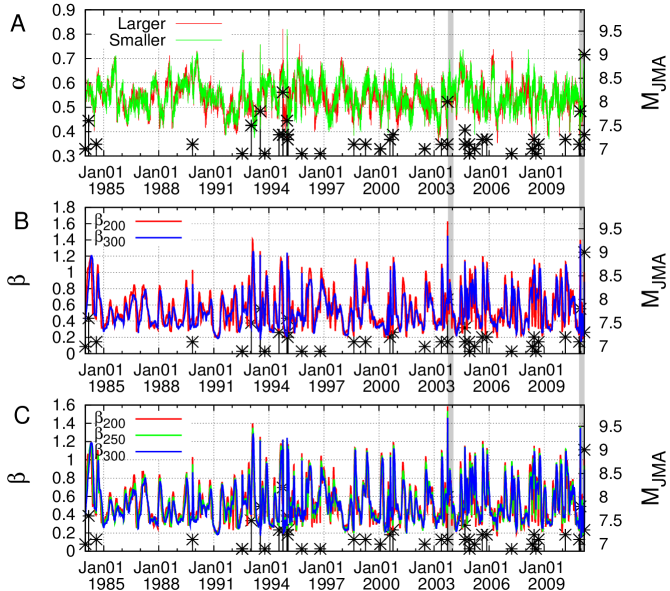
Figure 2: (color) The DFA exponent $\alpha$ and the variability $\beta$ of $\kappa_{1}$ (left scale) of seismicity since 1 January 1984 until just before the M9 Tohoku EQ: (A) the exponent $\alpha$ for $W$=300 in the larger area ${\rm N}_{25}^{46}$ ${\rm E}_{125}^{148}$ (red) and in the smaller area ${\rm N}_{25}^{46}$ ${\rm E}_{125}^{146}$ (green) of Fig.1. (B) The variability $\beta_{200}$ (red) and $\beta_{300}$ (blue) in the smaller area. (C) The variability $\beta_{200}$ (red), $\beta_{250}$ (green) and $\beta_{300}$ (blue) in the larger area. In addition, all ${\rm M}_{JMA}\geq 7.0$ EQs (in black, ${\rm M}_{JMA}$ in the right scale) are plotted.

Figure 2 provides an overview of the values computed in this study. In particular, the following quantities are plotted versus the conventional time during the 27 year period from 1 January 1984 until the Tohoku EQ occurrence on 11 March 2011: In Fig. 2A the DFA exponent $\alpha$ is depicted with red line for the larger area and with green line for the smaller. In Fig. 2B, we show the quantities $\beta_{200}$ and $\beta_{300}$ (in red and blue, respectively) for the smaller area. Finally, in Fig. 2C, we show $\beta_{200}$, $\beta_{250}$ and $\beta_{300}$ (in red, green and blue, respectively) for the larger area.

A first inspection of the $\alpha$ values in Fig. 2A shows that in view of their strong fluctuations it is very difficult to identify their correlations with EQs. A closer inspection, however, reveals the following striking point: The deeper minima of the $\alpha$ values (when considering the $\alpha$ values in both areas) are observed in the periods marked with grey shade which are very close to the occurrence of the stronger EQs in Japan during the last decade. These two EQs are (Table 1) the M9 Tohoku EQ on 11 March 2011 with an epicenter at $38.10^{o}$N $142.86^{o}$E and the M8 Off-Tokachi EQ on 26 September 2003 with an epicenter at $41.78^{o}$N $144.08^{o}$E . This instigated a more detailed investigation of the $\alpha$ values close to these two major EQs for which unfortunately precursory geoelectrical data are lacking (for the case of the M9 Tohoku EQ only geomagnetic data are available, see below). Thus, before presenting these two investigations and in order to better understand the results obtained, we first describe below a similar investigation for the case of the volcanic-seismic swarm activity in 2000 in the Izu Island region, Japan, in which as mentioned both datasets, i.e., SES activities and seismicity, are available.

IV.1 The case of the volcanic-seismic swarm in 2000 in the Izu Island region

Figure 3 is an excerpt of Fig. 2 in expanded time scale during the six month period from 1 January 2000 until 1 July 2000, which is the date of occurrence of an M6.5 EQ close to Niijima Island (yellow square in Fig.1). This EQ was preceded by an SES activity initiated on 26 April 2000 at a measuring station located at this island (Uyeda et al., 2002, 2009).

An inspection of Figs. 3A to 3C reveals the following three main features referring to the periods before, during, and after the observation of the precursory $\beta$ minimum:

Stage A marked in cyan: Putting the details aside, we observe in Fig. 3A that around 12 February 2000 the DFA exponent in both areas went down to a value markedly smaller than 0.5, i.e., $\alpha\approx 0.41$, in the smaller area and $\alpha\approx 0.43$ in the larger area. These $\alpha_{min,bef}$ values indicate anticorrelated behavior in the magnitude time series.

Stage B marked in yellow: Since the last days of March until the first days of June 2000, the exponent $\alpha$ becomes markedly larger than 0.5, i.e., around $\alpha\approx 0.57$, pointing to the development of long range temporal correlations. In Figs. 3B and 3C, we then observe that after the last days of March the variability $\beta$ exhibits a gradual decrease and a minimum $\beta_{W,min}$ appears on a date around the date of the initiation of the SES activity. In particular, in Fig. 3C, the relevant curve (green) for $\beta_{250}$ in the larger area minimizes on 25 April 2000 which is approximately the date of the initiation of the SES activity, reported by Uyeda et al. (2002, 2009), lying also very close to the date (21 April) at which in the smaller area the $\beta_{200}$ curve (red) in Fig. 3B minimizes. Thus, in short the minimum $\beta_{W,min}$, appears when $\alpha>0.5$ and hence when long range correlations (corr) have been developed in the EQ magnitude time series. The corresponding $\alpha$ values during the observation of the minima $\beta_{250,min}$ will be hereafter designated $\alpha_{corr}$. Hence, in this case $\alpha_{corr}\approx 0.57$.

Stage C marked in brown: Approximately on 10 June 2000, Fig. 3A shows that the DFA exponent decreases to a value around 0.5. This means that the previously established long range temporal correlations between EQ magnitudes break down to an almost random behavior. The value $\alpha\approx 0.5$ remains almost constant until the third week of June and shortly after the aforementioned M6.5 EQ on 1 July 2000 occurred.

IV.2 The M8 Off Tokachi EQ on 26 September 2003

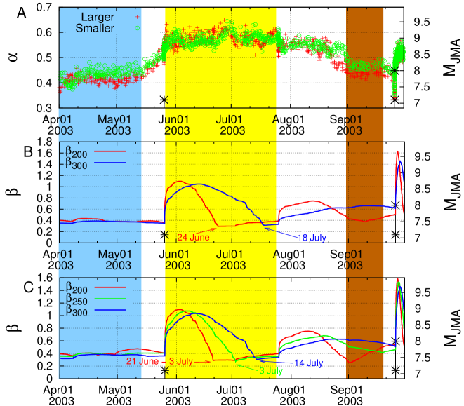
Figure 4: (color) Excerpt of Fig. 2 plotted in expanded time scale before the M8 Off Tokachi EQ on 26 September 2003

Figure 4 is an excerpt of Fig. 2 in expanded time scale which shows clearly what happened during an almost 6 month period before the occurrence of this major EQ. Using the same symbols as in the description of the previous case, the following three main features emerge from Figs. 4A to 4C:

(A) An anti-correlated behavior is evident in the cyan region in Fig. 4A lasting from 1 April until the first days of May 2003, since the corresponding $\alpha$ values resulting from both areas scatter around $\alpha=$0.42 and 0.44 for the larger and the smaller area, respectively.

(B) In the yellow region, i.e., from around the last days of May until almost the beginning of the last week of July 2003, long range correlations have been developed since the $\alpha$ values in Fig. 4A markedly exceed 0.5. The $\beta$ minima appear during this period (Tables 2 and 4), as can be seen in Figs.4C and 4B, and the corresponding $\alpha$ values are $\alpha_{corr}\approx 0.6$.

(C) A breakdown of long range correlations starts around 1 September 2003, see the beginning of the brown region in Fig.4A where the $\alpha$ values decrease to $\alpha\approx$0.5, i.e., close to random behavior, and subsequently go down to around $\alpha\approx$0.45 (while finally $\alpha$ reaches the value $\alpha_{min,aft}=$0.384 and 0.434 for the larger and the smaller area, respectively, see Tables 2 and 4) indicating anti-correlation. The M8 EQ occurred three weeks later, i.e., on 26 September 2003, and after its occurrence the $\alpha$ value decreases to an unusual low $\alpha$ value (0.33 and 0.35 in the larger and the smaller area, respectively), which corresponds to the one -out of the two- deeper $\alpha$ minima mentioned above in the periods marked with grey shade in Fig. 2A.

IV.3 The M9 Tohoku EQ on 11 March 2011

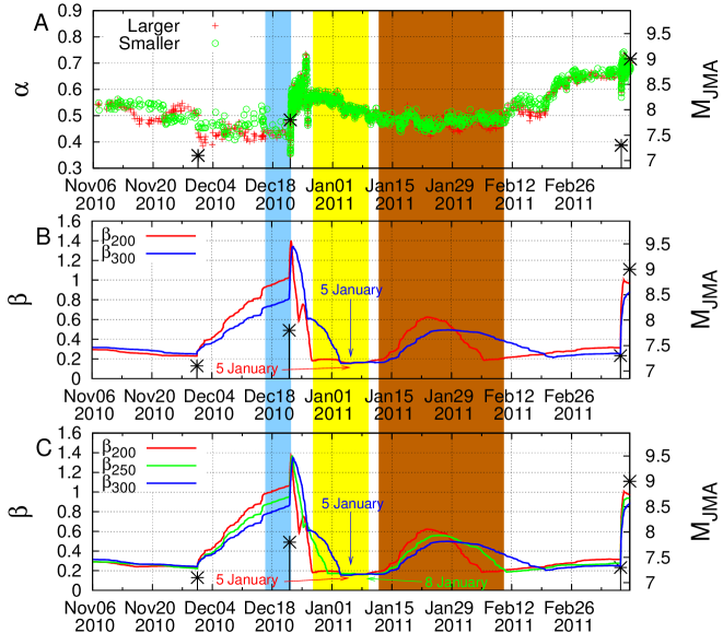
Figure 5: (color) Excerpt of Fig. 2 plotted in expanded time scale before the M9 Tohoku EQ on 11 March 2011.

Figure 5 is an almost four month excerpt of Fig. 2 in which one can visualize what happened before this super giant EQ. By the same token as in the previous cases, the following three main features are recognized:

(A) The cyan region in Fig. 5 corresponds to an anticorrelated behavior since in Fig. 5A the $\alpha$ values in both areas become markedly smaller than 0.5 after around 16 December 2010, including an evident minimum $\alpha_{min,bef}$ on 22 December 2010. This is one out of the two deeper $\alpha$ minima mentioned in Fig. 2A.

(B) In the yellow region, from about 23 December 2010 until around 8 January 2011, the $\alpha$ values depicted in Fig. 5A indicate the establishment of long range correlations since $\alpha>0.5$. In this region, and in particular during the last week of December 2010, the $\beta$ values in Figs. 5B and 5C show that an evident decrease starts leading to a deep $\beta$ minimum around 5 January 2011. This is the deepest $\beta_{W,min}$ observed (Sarlis et al., 2013) since the beginning of our investigation on 1 January 1984, as can be seen in the rightmost side of Figs. 2B and 2C. Remarkably, the anomalous magnetic field variations (Xu et al., 2013) (which accompany anomalous electric field variations, i.e., SES activities (Varotsos et al., 2003c)) initiated almost on the same date, i.e., 4 January 2011.

(C) In the brown region lasting from about 13 January to 10 February 2011, the behavior turns to an anti-correlated one, which is very close to random, as evidenced from Fig. 5A in which the $\alpha$ values are $\alpha\lesssim 0.5$. The M9 EQ occurred almost four weeks after this period, i.e., on 11 March 2011.

The following important comment referring to the two deeper minima of the $\alpha$ values in Fig. 2A is now in order: Here, the unusually low $\alpha_{min,bef}$ on 22 December 2010 (Fig. 5A) has been shortly followed by the deepest $\beta$ minimum on 5 January 2011 (Figs. 5B and 5C). This is of precursory nature. To the contrary, the unusually low $\alpha$ minimum value on 26 September 2003 discussed in the previous case -which has not been shortly followed by a deep $\beta$ minimum (see Fig. 2A)- is not precursory having been influenced by the preceding M8 Off Tokachi EQ. In other words, upon the observation of an unusually low $\alpha$ value, we cannot decide whether it is of precursory nature but we have to combine this observation with the results of natural time analysis and investigate whether this $\alpha_{min}$ value is shortly followed by a deep $\beta_{W,min}$ value. Hence, it is of key importance to examine in each case whether the sequence of the aforementioned three main features A, B, C has appeared or not.

V Discussion and conclusions

DFA has been employed long ago for the study of seimic time series in various regions, e.g. see Telesca et al. (2003) for the Italian territory. DFA studies of the long-term seismicity in Northern and Southern California were initially focused on the regimes of stationary seismic activity and found that long range correlations exist (Lennartz et al., 2008) between EQ magnitudes with $\alpha=0.6$. Similar DFA studies of long-term seismicity were later(Sarlis et al., 2010a, b) extended also to the seismic data of Japan and the results strengthened the existence of long range temporal correlations. In particular, it was found(Sarlis et al., 2010a, b) that the DFA exponent is around 0.6 for short scales but $\alpha=$0.8-0.9 for longer scales (the cross-over being around 200 EQs). In addition, the nonextensive statistical mechanics(Abe and Okamoto, 2001; Tsallis, 2009), pionered by Tsallis (1988), has been employed(Sarlis et al., 2010b) in order to investigate whether it can reproduce the observed seismic data fluctuations. In this framework, on the basis of which it has been shown (Livadiotis and McComas, 2009) that kappa distributions arise, a generalization of the Guternbeng-Richter (G-R) law for seicmicity has been offered (for details and relevant references see Section 6.5 of Varotsos et al. (2011a) as well as Telesca (2012)) and the investigation led to the following conclusions(Varotsos et al., 2011a; Sarlis et al., 2010b): The results of the natural time analysis of synthetic seismic data obtained from either the conventional G-R law or its nonextensive generalization, deviate markedly from those of the real seismic data. On the other hand, if temporal correlations between EQ magnitudes, with different $\alpha$ values (i.e., $\alpha\approx 0.6$ and $\alpha\approx$0.8-0.9 for short and long scales, respectively), will be inserted to the synthetic seismic data, the results of natural time analysis agree well with those obtained from the real seismic data. In other words, the parameter $q$ of nonextensive statistical mechanics cannot capture the whole effect of long range temporal correlations between the magnitudes of successive EQs. On the other hand, the nonextensive statistical mechanics, when combined with natural time analysis (which focuses on the sequential order of the events that appear in nature) does enable a satisfactory description of the fluctuations of the real data of long-term seismicity.

In the present paper, we study the dynamic evolution of seismicity and pay attention to the regimes before major EQs by combining the results of DFA of EQ magnitude time series with natural time analysis since the latter has revealed that a minimum $\beta_{W,min}$ in the fluctuations of the order parameter of seismicity is observed before major EQs in California (Varotsos et al., 2012) and Japan (Sarlis et al., 2013; Varotsos et al., 2013) (cf. The nonextensive statistical mechanics cannot serve for the purpose of the present study, i.e., follow the dynamic evolution of seismicity). This combination has been applied in the previous Section to three characteristic cases in Japan, i.e., the volcanic-seismic swarm activity in the Izu Island region in 2000, the M8 off Tokachi EQ in 2003 and the M9 Tohoku EQ in 2011. The following three main features have been found in all three cases:

Stage A(before the $\beta_{W,min}$): Clear anti-correlated behavior, $\alpha<0.5$

Stage B: Establishment of long range correlations, $\alpha>0.5$ during which a minimum $\beta_{W,min}$ appears (approximately at the date of the initiation of the SES activity as found in the Izu case as well as in the M9 Tohoku case).

Stage C (after the $\beta_{W,min}$): Breakdown of long range correlations with emergence of an almost random behavior turning to anti-correlation, $\alpha\lesssim 0.5$. A few weeks after this breakdown the major EQ occurs. This is strikingly reminiscent of the findings in other complex time series: In the case of electrocardiograms, for example, the long-range temporal correlations that characterize the healthy heart rate variability break down for individuals of high risk of sudden cardiac death and often accompanied by emergence of uncorrelated randomness (Varotsos et al., 2011a; Goldberger et al., 2002; Varotsos et al., 2007).

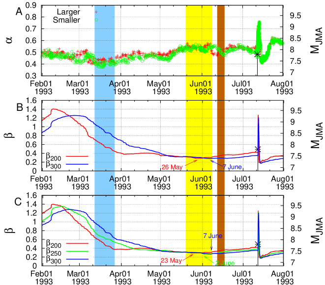
Figure 6: (color) Excerpt of Fig. 2 plotted in expanded time scale before the M7.8 Southwest-Off Hokkaido EQ on 12 July 1993.

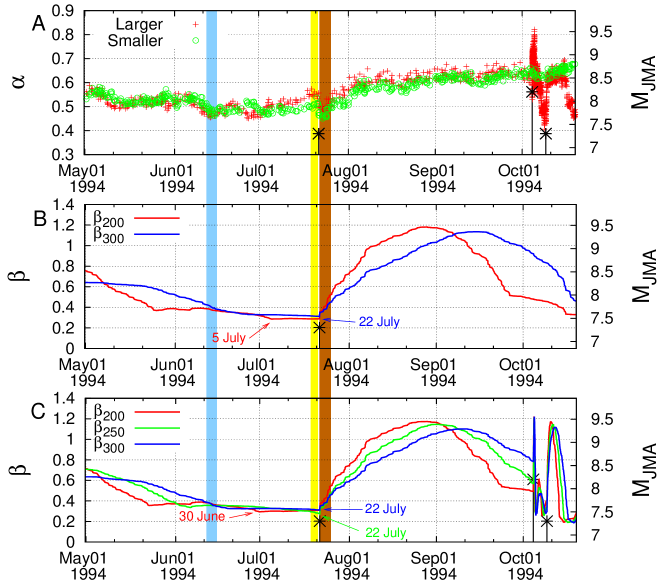
Figure 7: (color) Excerpt of Fig. 2 plotted in expanded time scale before the M8.2 East-Off Hokkaido EQ on 4 October 1994.

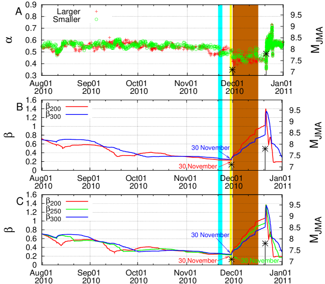
Figure 8: (color) Excerpt of Fig. 2 plotted in expanded time scale before the M7.8 Near Chichi-jima EQ on 22 December 2010.

The same features have been found to hold before all the other ${\rm M}_{JMA}\geq 7.8$ EQs in Japan during the period 1 January to the Tohoku EQ occurrence, i.e., the Southwest-Off Hokkaido M7.8 EQ in 1993 (Fig.6) the East-Off Hokkaido M8.2 EQ in 1994 (Fig. 7), and the Near Chichi-jima M7.8 EQ in 2010 (Fig. 8). As for the observed pattern in $\alpha$, i.e., anti-correlated, correlated and random, it might be related to the tectonics and geodynamics, but a precise physical justification of its origin is not yet clear.

The $\beta$ minima that are precursory to ${\rm M}_{JMA}\geq 7.8$ EQs can be distinguished from other $\beta$ minima that are either non-precursory or may be followed by EQs of smaller magnitude through the following procedure (for details see Appendix and Tables 2 to 5). We make separate studies for the two rectangular areas shown in Fig. 1, i.e., by analyzing the time series of EQs occurring in each area, first in the larger area and secondly in the smaller. In the study of each area, we do the following: We first identify the $\beta$ minima that appear a few months before all ${\rm M}_{JMA}\geq 7.8$ EQs and determine their $\beta_{300,min}/\beta_{200,min}$ values. These values lie in a certain narrow range close to unity. Among the remaining minima, we choose those which are equally deep or deeper than the shallowest one of the $\beta_{200,min}$ values that preceded the ${\rm M}_{JMA}\geq 7.8$ EQs and in addition they have $\beta_{300,min}/\beta_{200,min}$ values lying in the range determined above (see Appendix). In order for any of these minima to be precursory to ${\rm M}_{JMA}\geq 7.8$ EQs, beyond the fact that they should exhibit the three main features, A, B, C, mentioned above, they should also have the following property: They should appear practically on the same dates (differing by no more than 10 days or so) in the investigations of both areas. The application of the aforementioned procedure reveals (see Appendix) that only the $\beta$ minima appearing a few months before the five ${\rm M}_{JMA}\geq 7.8$ EQs exhibit all the aforementioned properties. Remarkably, this procedure (see Appendix) could have been applied before the occurrence of the M9 Tohoku EQ, after the identification of the deepest $\beta$ minimum observed on January 2011, leading to the conclusion that an ${\rm M}_{JMA}\geq 7.8$ EQ was going to occur in a few months.

Let us summarize: Here, by employing the DFA of the EQ magnitude time series we show that the minimum $\beta_{W,min}$ of the fluctuations of the order parameter of seismicity a few months before an ${\rm M}_{JMA}\geq 7.8$ EQ is observed when long range correlations prevail ($\alpha>0.5$). In addition, these $\beta_{W,min}$ is preceded by a stage in which DFA reveals clear anti-correlated behavior ($\alpha<0.5$) as well as it is followed by another stage in which long range correlations break down to an almost random behavior turning to anti-correlation ($\alpha\lesssim 0.5$). On the basis of these main features we suggest a procedure which distinguishes the $\beta$ minima that precede EQs of magnitude exceeding a certain threshold (i.e., ${\rm M}_{JMA}\geq 7.8$) from other $\beta$ minima which are either non-precursory or may be followed by EQs of smaller magnitude.

Appendix A Distinction of the $\beta$ minima that precede EQs of magnitude ${\rm M}_{JMA}\geq 7.8$ from other minima which are either non-precursory or followed by EQs of smaller magnitude

Recall that in order to classify a $\beta_{W,min}$ value, it should be a minimum for at least $W$ values before and $W$ values after. Further, to assure that $\beta_{200,min}$, $\beta_{250,min}$ and $\beta_{300,min}$ are precursory of the same mainshock and hence belong to the same critical process, almost all (in practice above 90$\%$ of) the events which led to $\beta_{200,min}$ should participate in the calculation of $\beta_{250,min}$ and $\beta_{300,min}$.

To distinguish the $\beta_{W,min}$ that are precursory to EQs of magnitude ${\rm M}_{JMA}\geq 7.8$ from other minima which are either non-precursory or may be followed by EQs of smaller magnitude, we make separate studies for the larger and the smaller area and the results obtained should be necessarily checked for their self-consistency. For example, a major EQ whose epicenter lies in both areas should be preceded by $\beta_{W,min}$ identified in the separate studies of these two areas approximately (in view of their difference in seismic rates) on the same date. In particular, we work as follows:

Let us assume that we start the investigation from the larger area where five EQs of magnitude 7.8 or larger occurred from 1 January 1984 until the M9 Tohoku EQ in 2011 (Table 1). We first identify the $\beta$ minima that appear a few months before all these EQs and determine their $\beta_{300,min}/\beta_{200,min}$ values (see Table 2). These values are found to lie in a narrow range close to unity (Sarlis et al., 2013), i.e., in the range 0.92-1.06. (This range slightly differs from the previously reported (Sarlis et al., 2013) range 0.95-1.08 since in the present work the numerical accuracy of the calculated $\kappa_{1}$ values for $W>100$ has been improved.) This is understood in the context that these values correspond to similar critical processes, thus exhibiting the same dependence of $\beta_{W}$ on $W$. During the whole period studied, however, beyond the above mentioned $\beta$ minima before all the ${\rm M}_{JMA}\geq 7.8$ EQs, more minima exist. Among these minima we choose those which are equally deep or deeper than the shallowest one of the $\beta_{200,min}$ values previously identified (e.g., 0.294 in Table 2) and in addition they have $\beta_{300,min}/\beta_{200,min}$ values lying in the narrow range determined above. Thus, we now find a list of “additional” $\beta$ minima (see Table 3) that must be checked whether they are non-precursory or may be followed by EQs of smaller magnitude.

We now repeat the whole procedure -as described above- for the determination of $\beta$ minima in the smaller area. Thus, we obtain a new set of $\beta$ minima (with shallowest $\beta_{200,min}$=0.293 and $\beta_{300,min}/\beta_{200,min}$ range 0.97-1.09, see Table 4) that appear a few months before all the ${\rm M}_{JMA}\geq 7.8$ EQs (cf. there exist 4 such EQs in the smaller area, see Fig.1) as well as a new list of “additional” $\beta$ minima (see Table 5) to be checked whether they are non-precursory or may be followed by EQs of smaller magnitude. Comparing these new $\beta$ minima with the previous ones, we investigate whether they:

(1) appear practically on the same date (differing by no more than 10 days or so) in both areas, and

(2) exhibit the three main features (i.e., the sequence (A) anti-correlated behavior / (B) correlated /(C) almost random behavior) emerged from the results of DFA of EQ magnitude time series discussed in the main text. In Tables 3 and 5 corresponding to the “additional” minima, we mark in bold the values which do not satisfy at least one of the three inequalities given below which quantify these three main features

$$\alpha_{min,bef}\leq 0.47,\alpha_{corr}>0.50,\alpha_{min,aft}\leq 0.50$$

(Note that considerable errors are introduced in the estimation of the $\alpha$ exponent when using a relatively small number of points as the one used here, i.e., 300. This is why we adopt $\alpha=0.47$ as the maximum value in order to assure anti-correlated behavior in the period before the appearance of $\beta$ minimum.)

A summary of the main results obtained after carrying out this investigation is as follows:

First, the $\beta$ minima identified a few months before all the ${\rm M}_{JMA}\geq 7.8$ EQs with epicenters inside of both areas obey the aforementioned requirements (1) and (2), see Tables 2 and 4. Remarkably, in the remaining case, i.e., the East-Off Hokkaido M8.2 EQ labelled EQ2 in Table 1, with an epicenter outside of the smaller area but inside the larger, we find $\beta$ minimum not only in the study of the larger area (on 30 June 1994, see Table 2), but also in the relevant study of the smaller area (see the third $\beta$ minimum in Table 5 observed on 5 July 1994). Second, all the other “additional” $\beta$ minima resulting from the studies in both areas (see Tables 3 and 5) violate at least one of the requirements (1) and (2). In other words, only the $\beta$ minima appearing a few months before the five ${\rm M}_{JMA}\geq 7.8$ EQs exhibit all the aforementioned properties. Remarkably, this procedure could have been applied before the occurrence of the M9 Tohoku EQ, after the identification of the deepest $\beta$ minimum on January 2011 having $\beta_{300,min}/\beta_{200,min}$ almost unity, thus lying inside the narrow ranges identified from previous ${\rm M}_{JMA}\geq 7.8$ EQs (see Tables 2 and 4), leading to the conclusion, as mentioned in the main text, that a ${\rm M}_{JMA}\geq 7.8$ EQ was going to occur in a few months.

We clarify that the above procedure does not preclude of course that one of the “additional” minima may be of truly precursory nature, but corresponding to an EQ of magnitude smaller than the threshold adopted. As a first example we mention the case marked FA7 in Table 3 referring to a $\beta_{200,min}$ observed on 12 April 2000. It preceded the M6.5 EQ that occurred on 1 July 2000 of the volcanic-seismic swarm activity in the Izu Island region in 2000, see the $\beta_{200}$ curve (red) in Fig.3C. A second example is the case marked EQc in Table 3, which refers to a $\beta_{200,min}$ on 15 October 1994 that preceded the M7.6 Far-Off Sanriku EQ on 28 December 1994 (Sarlis et al., 2013).

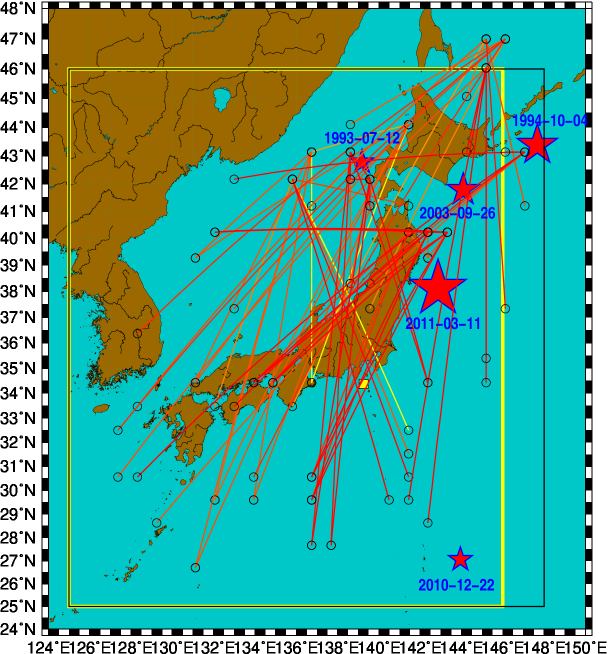
Figure 1: (color) The epicenters (stars) of all EQs with magnitude 7.8 or larger within the area ${\rm N}_{25}^{46}$ ${\rm E}_{125}^{148}$ (black rectangle) since 1 January 1984 until the M9 Tohoku EQ on 11 March 2011 (Table 1). The smaller area ${\rm N}_{25}^{46}$ ${\rm E}_{125}^{146}$ studied by Varotsos et al. (2013) is also shown with yellow rectangle. The small yellow square indicates the location of the Niijima Island where the precursory SES activity of the volcanic-seismic swarm activity in 2000 in the Izu Island region has been recorded (Uyeda et al., 2002, 2009). Furthermore, the network links as reported by Tenenbaum et al. (2012) (see their Fig.6(a)) are also shown.

Figure 3: (color) (A)-(C): Excerpt of Fig. 2 plotted in expanded time scale from 1 January 2000 until 1 July 2000, which is the date of occurrence of the M6.5 EQ close to Niijima Island during the volcanic-seismic swarm activity in the Izu Island region in 2000.

Table 1: All ${\rm M}_{JMA}\geq 7.8$ EQs since 1 January 1984 until the M9 Tohoku EQ on 11 March 2011 in the larger area ${\rm N}_{25}^{46}{\rm E}_{125}^{148}$

Label	EQ Date	EQ name	Lat. (oN)	Lon. (oE)	M
EQ1	1993-07-12	Southwest-Off Hokkaido EQ	42.78	139.18	7.8
EQ2	1994-10-04	East-Off Hokkaido EQ	43.38	147.67	8.2
EQ3	2003-09-26	Off Tokachi EQ	41.78	144.08	8.0
EQ4	2010-12-22	Near Chichi-jima EQ	27.05	143.93	7.8
EQ5	2011-03-11	Tohoku EQ	38.10	142.86	9.0

This EQ lies outside of the smaller area ${\rm N}_{25}^{46}{\rm E}_{125}^{146}$.

Table 2: The values of $\beta_{W,min}$, $\alpha_{min,bef}$, $\alpha_{corr}$ and $\alpha_{min,aft}$ in the larger area investigated with sliding natural time windows of length 6 to $W$ that preceded the ${\rm M}_{JMA}\geq 7.8$ EQs listed in Table 1. Hereafter, the value of $\alpha_{corr}$ is given when $\beta_{250,min}$ appears and $\alpha_{min,bef}$ is the minimum of the DFA exponent up to three and a half months (105 days) before $\beta_{250,min}$.

Label	$\beta_{200,min}$	$\beta_{250,min}$	$\beta_{300,min}$	$\frac{\beta_{300,min}}{\beta_{200,min}}$	$\alpha_{min,bef}$	$\alpha_{corr}$	$\alpha_{min,aft}$
EQ1	0.292(19930523)	0.266(19930602)	0.270(19930607)	0.92	0.397(19930327)	0.515(19930602)	0.469(19930613)
EQ2	0.294(19940630)	0.274(19940722)	0.312(19940722)	1.06	0.451(19940627)	0.557(19940722)	0.476(19940724)
EQ3	0.289(20030703)	0.273(20030703)	0.307(20030714)	1.06	0.356(20030325)	0.553(20030703)	0.384(20030925)
EQ4	0.233(20101130)	0.221(20101130)	0.242(20101130)	1.04	0.467(20101116)	0.501(20101130)	0.385(20101201)
EQ5	0.156(20110105)	0.160(20110108)	0.154(20110105)	0.99	0.348(20101222)	0.524(20110108)	0.422(20110123)

A comparable (within $\pm 0.0005$) value $\beta_{200,min}=$0.293 is also found on 24 May 1993.
The same (within $\pm 0.0005$) value $\beta_{200,min}=$0.289 is also found on 21 June 2003.
The date of the M8 EQ is either 25 or 26 September 2003 depending on the use of LT or UT, respectively. Here, we use LT. This value of $\alpha$ is observed 15.5 hours before the mainshock.

Table 3: The values of $\beta_{W,min}$, $\alpha_{min,bef}$, $\alpha_{corr}$ and $\alpha_{min,aft}$ for the “additional” minima identified in the larger area investigated with sliding natural time windows of length 6 to $W$

Label	$\beta_{200,min}$	$\beta_{250,min}$	$\beta_{300,min}$	$\frac{\beta_{300,min}}{\beta_{200,min}}$	$\alpha_{min,bef}$	$\alpha_{corr}$	$\alpha_{min,aft}$
FA1	0.253(19861013)	0.256(19861028)	0.246(19861115)	0.97	0.484(19860905)	0.557(19861028)	0.446(19861129)
FA2	0.279(19890808)	0.282(19890826)	0.285(19890915)	1.02	0.524(19890730)	0.566(19890826)	0.508(19891128)
FA3	0.251(19920405)	0.242(19920423)	0.247(19920510)	0.98	0.389(19920325)	0.411(19920423)	0.411(19920423)
FA4	0.187(19930713)	0.176(19930714)	0.174(19930715)	0.93	0.441(19930407)	0.584(19930714)	0.410(19930716)
EQc	0.194(19941015)	0.191(19941017)	0.188(19941019)	0.97	0.406(19941009)	0.584(19941017)	0.399(19941125)
FA5	0.236(19980217)	0.214(19980228)	0.223(19980312)	0.95	0.524(19980211)	0.540(19980228)	0.470(19980509)
FA6	0.281(19981218)	0.299(19981230)	0.294(19990110)	1.05	0.423(19981223)	0.474(19981230)	0.457(19990108)
FA7	0.227(20000412)	0.211(20000425)	0.213(20000506)	0.94	0.411(20000129)	0.571(20000425)	0.411(20000702)
FA8	0.243(20020512)	0.231(20020523)	0.253(20020603)	1.04	0.495(20020515)	0.527(20020523)	0.424(20020630)
FA9	0.233(20040221)	0.224(20040302)	0.219(20040315)	0.94	0.478(20031224)	0.512(20040302)	0.447(20040319)
FA10	0.283(20050611)	0.305(20050620)	0.300(20050701)	1.06	0.413(20050320)	0.460(20050620)	0.430(20050620)
FA11	0.267(20080227)	0.287(20080227)	0.284(20080227)	1.06	0.507(20080103)	0.668(20080227)	0.360(20080508)

The values shown in bold violate at least one of the main three features $\alpha_{min,bef}\leq 0.47$, $\alpha_{corr}>0.50$, $\alpha_{min,aft}\leq 0.50$
This minimum was followed by the M7.6 Far-Off Sanriku EQ on 28 December 1994, see Sarlis et al. (2013)
The same (within $\pm 0.0005$) value $\beta_{200,min}=$0.227 is also found on 13 April 2000.
This value and date of $\alpha_{min,bef}$ results of course when solely considering the DFA exponent in the larger area. Upon demanding however a common behavior of the DFA exponent in both areas, we find the result described in the text which is marked in Fig.3 in cyan.

Table 4: The values of $\beta_{W,min}$, $\alpha_{min,bef}$, $\alpha_{corr}$ and $\alpha_{min,aft}$ in the smaller area ${\rm N}_{25}^{46}{\rm E}_{125}^{146}$ investigated with sliding natural time windows of length 6 to $W$ that preceded ${\rm M}_{JMA}\geq 7.8$ EQs.

Label	$\beta_{200,min}$	$\beta_{250,min}$	$\beta_{300,min}$	$\frac{\beta_{300,min}}{\beta_{200,min}}$	$\alpha_{min,bef}$	$\alpha_{corr}$	$\alpha_{min,aft}$
EQ1	0.288(19930526)	0.264(19930607)	0.278(19930607)	0.97	0.374(19930319)	0.557(19930607)	0.473(19930617)
EQ3	0.293(20030624)	0.311(20030709)	0.309(20030718)	1.06	0.374(20030408)	0.570(20030709)	0.434(20030925)
EQ4	0.228(20101130)	0.233(20101130)	0.250(20101130)	1.09	0.467(20101122)	0.516(20101130)	0.408(20101209)
EQ5	0.156(20110105)	0.160(20110108)	0.154(20110105)	0.99	0.354(20101222)	0.522(20110108)	0.439(20110117)

The epicenter of EQ2 -not included here- lies outside of the smaller area.
The date of the M8 EQ is either 25 or 26 September 2003 depending on the use of LT or UT, respectively. Here, we use LT. This value of $\alpha$ is observed 24.5 hours before the mainshock.

Table 5: The values of $\beta_{W,min}$, $\alpha_{min,bef}$, $\alpha_{corr}$ and $\alpha_{min,aft}$ for the “additional” minima identified in the smaller area investigated with sliding natural time windows of length 6 to $W$

Label	$\beta_{200,min}$	$\beta_{250,min}$	$\beta_{300,min}$	$\frac{\beta_{300,min}}{\beta_{200,min}}$	$\alpha_{min,bef}$	$\alpha_{corr}$	$\alpha_{min,aft}$
Fa1	0.276(19890810)	0.278(19890830)	0.294(19890921)	1.06	0.516(19890805)	0.589(19890830)	0.513(19891129)
Fa2	0.263(19920412)	0.261(19920503)	0.264(19920520)	1.00	0.409(19920330)	0.474(19920503)	0.465(19920507)
Fa3	0.286(19940705)	0.297(19940722)	0.310(19940722)	1.09	0.461(19940615)	0.501(19940722)	0.451(19940723)
EQc	0.205(19941128)	0.211(19941210)	0.212(19941227)	1.03	0.539(19941109)	0.615(19941210)	0.478(19941228)
Fa4	0.252(19950511)	0.238(19950519)	0.262(19950528)	1.04	0.441(19950204)	0.566(19950519)	0.436(19950702)
Fa5	0.220(19980227)	0.230(19980313)	0.222(19980330)	1.01	0.481(19980301)	0.536(19980313)	0.490(19980423)
Fa6	0.238(20070701)	0.249(20070701)	0.240(20070701)	1.01	0.437(20070609)	0.523(20070701)	0.454(20070720)

The values shown in bold violate at least one of the main three features $\alpha_{min,bef}\leq 0.47$, $\alpha_{corr}>0.50$, $\alpha_{min,aft}\leq 0.50$
The same (within $\pm 0.0005$) value $\beta_{200,min}=$0.263 is also found on 13 April 1992.
This minimum was followed by EQ2 which has an epicenter outside of the smaller area (but inside the larger).
This minimum was followed by the M7.6 Far-Off Sanriku EQ on 28 December 1994, see Sarlis et al. (2013).
The same (within $\pm 0.0005$) value $\beta_{200,min}=$0.205 is also found on 30 November 1994.
The same (within $\pm 0.0005$) value $\beta_{200,min}=$0.252 is also found on 12 May 1995.