Finite Size Scaling in the Kuramoto Model

Abstract

We investigate the scaling properties of the order parameter and the largest nonvanishing Lyapunov exponent for the fully locked state in the Kuramoto model with a finite number $N$ of oscillators. We show that, for any finite value of $N$, both quantities scale as $(K-K_{L})^{1/2}$ with the coupling strength $K$ sufficiently close to the locking threshold $K_{L}$. We confirm numerically these predictions for oscillator frequencies evenly spaced in the interval $[-1,1]$ and additionally find that the coupling range $\delta K$ over which this scaling is valid shrinks like $\delta K\sim N^{-\alpha}$ with $\alpha\approx 1.5$ as $N\rightarrow\infty$. Away from this interval, the order parameter exhibits the infinite-$N$ behavior $r-r_{L}\sim(K-K_{L})^{2/3}$ proposed by Pazó [Pazo2005]. We argue that the crossover between the two behaviors occurs because at the locking threshold, the upper bound of the continuous part of the spectrum of the fully locked state approaches zero as $N$ increases. Our results clarify the convergence to the $N\rightarrow\infty$ limit in the Kuramoto model.

I Introduction

The coupled oscillator model introduced by Kuramoto in the late 70’s has established itself as a paradigmatic model for the study of synchronization phenomena, where it opened a vast area of research. The Kuramoto model allows to investigate the interplay between the tendency that individual oscillators have to run at their natural frequency and a sinusoidal all-to-all coupling which attempts to synchronize the oscillators Kuramoto (1975, 1984). Kuramoto elegantly solved the model in the limit of infinitely many oscillators with natural frequencies drawn from a Lorentzian distribution, for which he showed that upon increasing the coupling between oscillators, the system undergoes a transition from an incoherent disordered phase to a partially synchronized state with a finite fraction of oscillators rotating in unison Kuramoto (1975, 1984); Strogatz (2000).

Several evolutions of the original Kuramoto model have been investigated, including models with different natural frequency distributions, with couplings defined on a complex network topology, oscillators with inertia, couplings with frustration, with time delays and even negative couplings to name but a few Acebrón et al. (2005); Arenas et al. (2008). Such extensions are motivated by the connection that the Kuramoto model has with several physical systems, ranging from synchronization phenomena in biological systems Winfree (1967); Ermentrout (1991) to Josephson junction arrays Wiesenfeld et al. (1996), via synchronous AC electric power systems Dörfler et al. (2013); Motter et al. (2013); Coletta et al. (2016).

Recently, there has been a renewed interest in the finite size behavior of the Kuramoto model Mirollo and Strogatz (2005); Aeyels and Rogge (2004); Jadbabaie et al. (IEEE, Piscataway, NJ, 2004); Pazó (2005); Ottino-Löffler and Strogatz (2016). The problem is of interest, because all physically relevant systems and numerical simulations deal with a finite number $N$ of oscillators, which makes finding solutions to the Kuramoto model mathematically more involved. In particular, at finite $N$, the continuum limit breaks down so that self consistent equations for physically relevant quantities such as the order parameter can no longer be written in a mathematically convenient integral form. Important steps forward in the understanding of the finite size Kuramoto model include the description of the Lyapunov spectrum for the fully locked state as well as estimates of the critical coupling necessary for synchronization to occur Mirollo and Strogatz (2005); Aeyels and Rogge (2004); Jadbabaie et al. (IEEE, Piscataway, NJ, 2004). A complete understanding of the transition to the infinite-$N$ behavior is however still lacking.

In this work we consider the finite size Kuramoto model [Kuramoto, 1975, 1984] on the complete graph $\mathcal{G}$ with $N$ nodes and $|\mathcal{E}|=N(N-1)/2$ edges

$$\dot{\theta_{i}}=\omega_{i}+\frac{K}{N}\sum_{j=1}^{N}\sin\left(\theta_{j}-\theta_{i}\right)\,,\quad i=1,\dots,N\,,$$ (1)

where $\theta_{i}$ and $\omega_{i}$ are the phases and the natural frequencies of the oscillators, respectively, and $K/N>0$ is the coupling strength. For natural frequencies defined on a bounded interval, there exists a critical value of the coupling $K_{L}^{N}$ for which the system is in a fully locked state where all oscillators synchronize, with $K_{L}^{N}\rightarrow K_{L}^{\infty}$ as $N\rightarrow\infty$ Strogatz (2000); van Hemmen and Wreszinski (1993); Dörfler and Bullo (2011); Verwoerd and Mason (2011). For the particular case of uniformly distributed frequencies, the main focus of this work, it has been found that the transition from the incoherent state to full synchrony is of first order Pazó (2005). We investigate the scaling properties of the Lyapunov spectrum characterizing the linear stability of the fully locked state, and of the order parameter introduced by Kuramoto Kuramoto (1975, 1984). We show that above the locking threshold the largest non vanishing Lyapunov exponent $\lambda_{2}$ scales like $\lambda_{2}\sim(K-K_{L})^{1/2}$. Relating the expression for the order parameter $r$ [Eq. (2) below] to the Lyapunov exponents, we show that the order parameter also scales as $r-r_{L}\sim(K-K_{L})^{1/2}$, $r_{L}\equiv r(K_{L})$ being the order parameter at the locking threshold. We confirm numerically these results for uniformly distributed oscillator frequencies. At first glance, our results disagree with Pazó who obtained $r-r_{L}\sim(K-K_{L})^{2/3}$ Pazó (2005). The two results can be reconciled once one realizes that Pazó’s calculation is strictly valid for an infinite number of oscillators only, while our results are derived for finite $N$. We find numerically that our finite $N$ result is always valid close enough to $K_{L}$. However, its range of validity $\delta K$ becomes narrower and narrower as $N$ increases, with numerical data consistent with $\delta K\sim N^{-\alpha}\,,\alpha\approx 1.5$. We further argue that the crossover is triggered by the dependence on $N$ of the next largest non vanishing Lyapunov exponent $\lambda_{3}$ at $K_{L}$, $\lambda_{3}(K_{L})\sim N^{-1/2}$. Corrections to our results being of order $\lambda_{3}^{-1}$, they can no longer be neglected as $N\rightarrow\infty$. A side result of our approach is that all Lyapunov exponents of the fully locked state of the Kuramoto model are monotonically decreasing functions of the coupling strength. This directly implies that the linear stability of the fully locked state improves as the oscillator coupling is increased and that if the locked state exists at $K_{0}$, it exists at all coupling strengths $K\geq K_{0}$. We note that this result could have been anticipated starting from the properties of the Lyapunov spectrum discussed in Ref. Mirollo and Strogatz (2005).

This paper is organized as follows. Section II recalls the definition of fully locked states in the Kuramoto model. Sections III and IV present the calculation of the monotonicity of the Lyapunov exponents as a function of the coupling constant. Section V discusses the behavior of the largest nonvanishing Lyapunov exponent and of the order parameter in the immediate vicinity of the phase-locking threshold for a large but finite number of oscillators.

II The Kuramoto model

We consider the Kuramoto model defined by Eq. (1) and $\omega_{i}\in[-1,1]$ though our results remain valid for distributions defined on bounded intervals. Introducing the order parameter Kuramoto (1975, 1984)

$$re^{i\psi}=\frac{1}{N}\sum_{i=1}^{N}e^{i\theta_{i}}\,,$$ (2)

Eq. (1) can be rewritten as

$$\dot{\theta_{i}}=\omega_{i}+Kr\sin\left(\psi-\theta_{i}\right)\,,\quad i=1,\dots,N.$$ (3)

Given the invariance of the Kuramoto model under a global shift of all phases, we can set $\psi=0$. Without loss of generality we consider natural frequencies such that $\sum_{i}\omega_{i}=0$, which is tantamount to considering the system in a rotating frame. For $K>K_{L}$, Eq. (1) admits stationary solutions $\{\theta_{i}^{(0)}\}$ given by

$$\sin\left(\theta_{i}^{(0)}\right)=\frac{\omega_{i}}{Kr}\,,\quad i=1,\dots,N\,.$$ (4)

They are referred to as fully locked states. The linear stability of fully locked states is governed by the spectrum of the stability matrix $\bm{M}$, obtained by linearizing Eq. (1) close to $\{\theta_{i}^{(0)}\}$, and defined as

$$M_{ij}=\left\{\begin{array}[]{cl}\displaystyle\frac{K}{N}\cos\left(\theta_{j}^{(0)}-\theta_{i}^{(0)}\right)\,,&i\neq j\,,\\[8.53581pt] \displaystyle-\frac{K}{N}\sum_{l\neq i}\cos\left(\theta_{l}^{(0)}-\theta_{i}^{(0)}\right)\,,&i=j\,.\end{array}\right.$$ (5)

Since the stationary solutions of Eq. (1) are invariant under a global rotation of all angles, one of the eigenvalues of $\bm{M}$ is identical to zero. A stationary solution $\{\theta^{(0)}_{i}\}$ is linearly stable as long as $\bm{M}$ is negative semidefinite. This condition ensures that for any small perturbation around $\{\theta^{(0)}_{i}\}$, the system’s state, subject to the dynamics of Eq. (1), returns to $\{\theta^{(0)}_{i}\}$ exponentially fast. The eigenvalues $\lambda_{i}$ of $\bm{M}$ are referred to as the Lyapunov exponents and the linear stability condition is expressed as

$$\lambda_{1}=0>\lambda_{2}\geq\lambda_{3}\dots\geq\lambda_{N}\,.$$ (6)

In what follows $\{{\bm{u}}^{(q)}\}$, $q=1,\ldots,N$ is the othonormal basis of eigenvectors of $\bm{M}$ defined by $\bm{M}{\bm{u}}^{(q)}=\lambda_{q}{\bm{u}}^{(q)}$. In particular $\bm{u}^{(1)}=(1,\dots,1)/\sqrt{N}$ is the eigenvector associated with $\lambda_{1}=0$.

According to Sylvester’s criterion, a necessary condition for $\bm{M}$ to be negative semidefinite is that all its diagonal elements are negative (i.e. $M_{ii}\leq 0$ for all $i$). This implies [Mirollo and Strogatz, 2005]

$$\begin{array}[]{c}\displaystyle-\frac{K}{N}\sum_{l\neq i}\cos\left(\theta_{l}^{(0)}-\theta_{i}^{(0)}\right)=\displaystyle-\frac{K}{N}\left[\sum_{l=1}^{N}\cos\left(\theta_{l}^{(0)}-\theta_{i}^{(0)}\right)-1\right]\leq 0\\[8.53581pt] \displaystyle\Rightarrow-Kr\cos\left(\theta_{i}^{(0)}\right)+\frac{K}{N}\leq 0\\[8.53581pt] \displaystyle\Rightarrow 0\leq\frac{1}{rN}\leq\cos\left(\theta_{i}^{(0)}\right)\,,\quad\forall i=1,\ldots N\,.\end{array}$$ (7)

The positivity of the cosine, together with Eq. (4), allows to rewrite

$$\cos\left(\theta_{i}^{(0)}\right)=\sqrt{1-(\omega_{i}/Kr)^{2}}\,,\quad\forall i=1,\ldots N\,.$$ (8)

This choice actually corresponds to the unique stable locked state solution of the all-to-all Kuramoto model Mirollo and Strogatz (2005); Aeyels and Rogge (2004).

III Monotonicity of the order parameter

In this section we show that for the stable fully locked state the magnitude of the order parameter $r$ grows monotonically as the coupling constant $K$ increases. This result has already been reported in the literature [Jadbabaie et al., IEEE, Piscataway, NJ, 2004; Mirollo and Strogatz, 2005], however our calculation below is based on a novel formalism which we will use later on. We therefore present it.

We start by expressing the square of the modulus of the order parameter as

$$r^{2}=\frac{1}{N^{2}}\left[N+2\sum_{j>i}\cos\left(\theta_{j}^{(0)}-\theta_{i}^{(0)}\right)\right]\,,$$ (9)

where the sum runs over all pairs of oscillators. Taking the derivative of Eq. (9) with respect to $K$ gives

$$\frac{dr}{dK}=-\frac{1}{rN^{2}}\sum_{j>i}\sin\left(\theta_{j}^{(0)}-\theta_{i}^{(0)}\right)\frac{d}{dK}\left(\theta_{j}^{(0)}-\theta_{i}^{(0)}\right)\,.$$ (10)

To obtain an expression for $d\left.\left(\theta_{j}^{(0)}-\theta_{i}^{(0)}\right)\right/dK$, we take the derivative of the stationary condition

$$0=\omega_{i}+\frac{K}{N}\sum_{j=1}^{N}\sin\left(\theta_{j}^{(0)}-\theta_{i}^{(0)}\right)$$ (11)

with respect to $K$. This gives

$$\begin{array}[]{c}\displaystyle-\sum_{j=1}^{N}\sin\left(\theta^{(0)}_{j}-\theta^{(0)}_{i}\right)=K\sum_{j=1}^{N}\cos\left(\theta^{(0)}_{j}-\theta^{(0)}_{i}\right)\frac{d}{dK}\left(\theta_{j}^{(0)}-\theta_{i}^{(0)}\right)\\[8.53581pt] \Rightarrow\displaystyle\bm{\omega}/K={\bm{M}}\frac{d}{dK}{\bm{\theta}}^{(0)}\,,\end{array}$$ (12)

where ${\bm{\theta}}^{(0)}=(\theta^{(0)}_{1},\dots,\theta^{(0)}_{N})$ and ${\bm{\omega}}=(\omega_{1},\dots,\omega_{N})$. Since $\bm{M}$ is singular, we invert Eq. (12) using the Moore-Penrose pseudoinverse of $\bm{M}$ defined as

$${\bm{M}}^{-1}={\bm{T}}\left(\begin{array}[]{cccc}0&&&\\ &\lambda_{2}^{-1}&&\\ &&\ddots&\\ &&&\lambda_{N}^{-1}\end{array}\right){\bm{T}}^{\top}\,,$$ (13)

where ${\bm{T}}=(\bm{u}^{(1)},\ldots,\bm{u}^{(N)})$ and ${\bm{M}}^{-1}{\bm{M}}={\bm{M}}{\bm{M}}^{-1}=\mathbb{I}-\bm{u}^{(1)}{\bm{u}^{(1)}}^{\top}$. Multiplying Eq. (12) by ${\bm{M}}^{-1}$ yields

$$\frac{d}{dK}{\bm{\theta}}^{(0)}={\bm{M}}^{-1}\frac{\bm{\omega}}{K}+\frac{1}{N}\frac{d}{dK}\left(\begin{array}[]{c}\sum_{l}\theta_{l}^{(0)}\\ \vdots\\ \sum_{l}\theta_{l}^{(0)}\\ \end{array}\right)\,.$$ (14)

Finally, the difference between any two components of the expression above is given by

$$\begin{array}[]{lll}\displaystyle\frac{d}{dK}\left(\theta_{j}^{(0)}-\theta_{i}^{(0)}\right)&=&\displaystyle\frac{1}{K}\sum_{k}\left(M^{-1}_{jk}-M^{-1}_{ik}\right)\omega_{k}\\ &=&\displaystyle\frac{1}{K}\sum_{k,\,l\geq 2}\left(u_{j}^{(l)}-u_{i}^{(l)}\right)\frac{1}{\lambda_{l}}u_{k}^{(l)}\omega_{k}\,,\end{array}$$ (15)

where the terms with $\sum_{l}\theta_{l}^{(0)}$ in Eq. (14) drop due to the global rotational invariance of the Kuramoto model. Injecting this result into Eq. (10) gives

$$\frac{dr}{dK}=-\frac{1}{rKN^{2}}\sum_{\begin{subarray}{c}j>i\\ k,\,l\geq 2\end{subarray}}\frac{1}{\lambda_{l}}\sin\left(\theta_{j}^{(0)}-\theta_{i}^{(0)}\right)\left(u_{j}^{(l)}-u_{i}^{(l)}\right)u_{k}^{(l)}\omega_{k}\,.$$ (16)

In order to determine the sign of the right-hand side of Eq. (16) it is useful to introduce the incidence matrix $\bm{B}$ of the network. Given a graph $\mathcal{G}$ of $N$ nodes and $|\mathcal{E}|$ edges and given an arbitrary orientation of each edge, the incidence matrix $\bm{B}\in\rm I\!R^{N\times|\mathcal{E}|}$ is defined as follows

$$\begin{array}[]{ccc}B_{il}=\left\{\begin{array}[]{cl}1\,,&\textrm{if }i\textrm{ is the source of edge }l\,,\\ -1\,,&\textrm{if }i\textrm{ is the sink of edge }l\,,\\ 0\,,&\textrm{otherwise}\,.\\ \end{array}\right.\end{array}$$ (17)

The product ${\bm{B}}^{\top}{\bm{\theta}}^{(0)}$ is a vector in $\rm I\!R^{|\mathcal{E}|}$ whose $l^{\textrm{th}}$ entry is equal to $\theta_{i}^{(0)}-\theta_{j}^{(0)}$ where $i$ and $j$ are the nodes connected by edge $l$, and where the sign of this difference depends on the arbitrary choice of orientation of the edge ($i$ is the source and $j$ is the sink in this case). Similarly, given a vector $\bm{v}\in{\rm I\!R}^{|\mathcal{E}|}$, the product $\bm{B}{\bm{v}}$ is a vector in $\rm I\!R^{N}$ whose $i^{\textrm{th}}$ entry is equal to the sum $\sum_{l}\pm v_{l}$ over all edges $l$ connected to node $i$, and with the sign $\pm$ fixed by the nature (sink or source) of site $i$.

We then rewrite the Kuramoto model, Eq. (1), in vector form using the incidence matrix we just introduced

$$\dot{\bm{\theta}}={\bm{\omega}}-\frac{K}{N}{\bm{B}}\cdot\bm{\mathrm{sin}}\left({\bm{B}}^{T}\bm{\theta}\right)\,,$$ (18)

where we defined $\bm{\mathrm{sin}}({\bm{x}})\equiv(\sin(x_{1}),\dots,\sin(x_{|\mathcal{E}|}))$ for $\bm{x}\in\rm I\!R^{|\mathcal{E}|}$. Thus, for a stationary solution we have

$${\bm{\omega}}=\frac{K}{N}{\bm{B}}\cdot\bm{\mathrm{sin}}\left({\bm{B}}^{T}\bm{\theta}^{(0)}\right)\,.$$ (19)

This compact formulation allows to write

$$\begin{array}[]{lll}\displaystyle\sum_{k}u_{k}^{(l)}\omega_{k}&=&\displaystyle\frac{K}{N}\left({\bm{B}}^{\top}{\bm{u}}^{(l)}\right)^{T}\cdot\bm{\mathrm{sin}}\left({\bm{B}}^{T}\bm{\theta}^{(0)}\right)\\[8.53581pt] &=&\displaystyle\frac{K}{N}\sum_{j>i}\left(u_{i}^{(l)}-u_{j}^{(l)}\right)\sin\left(\theta^{(0)}_{i}-\theta^{(0)}_{j}\right)\,.\end{array}$$ (20)

Injecting this last identity into Eq. (16) gives for the fully locked state

$$\frac{dr}{dK}=-\frac{1}{rK^{2}N}\sum_{l\geq 2}\frac{1}{\lambda_{l}}\left(\sum_{k}{u_{k}^{(l)}\omega_{k}}\right)^{2}\geq 0\,,$$ (21)

since $r\geq 0$ and $\lambda_{l}<0$ for $l\geq 2$ in the stable fully locked state. The order parameter is therefore a monotonously increasing function of $K$.

IV Monotonicity of the Lyapunov exponents

Next, given the stable fully locked state $\{\theta^{(0)}_{i}\}$, we compute the variation of its Lyapunov exponents as a function of the coupling strength $K$. Because ${\bm{M}}$ is real and symmetric, we can apply the Hellmann-Feynmann theorem Cohen-Tannoudji et al. (1977) to calculate $d\lambda_{q}/dK$. We obtain

$$\frac{d\lambda_{q}}{dK}={\bm{u}^{(q)}}^{\top}\frac{d{\bm{M}}}{dK}\bm{u}^{(q)}\,.$$ (22)

We express the derivative of the stability matrix with respect to $K$ as $d{\bm{M}}/dK={\bm{M}}/K+\bar{{\bm{M}}}$, which injected back into Eq. (22) yields

$$\frac{d\lambda_{q}}{dK}=\frac{\lambda_{q}}{K}+{\bm{u}^{(q)}}^{\top}\bar{{\bm{M}}}\bm{u}^{(q)}\,.$$ (23)

The matrix $\bar{{\bm{M}}}$ is defined by

$$\bar{M}_{ij}=\left\{\begin{array}[]{cl}\displaystyle-\frac{K}{N}\sin\left(\theta_{j}^{(0)}-\theta_{i}^{(0)}\right)\frac{d}{dK}\left(\theta_{j}^{(0)}-\theta_{i}^{(0)}\right)\,,&i\neq j\,,\\[8.53581pt] \displaystyle\frac{K}{N}\sum_{l\neq i}\sin\left(\theta_{l}^{(0)}-\theta_{i}^{(0)}\right)\frac{d}{dK}\left(\theta_{j}^{(0)}-\theta_{i}^{(0)}\right)\,,&i=j\,.\end{array}\right.$$ (24)

Next we show that for the linearly stable fully locked state, $d\lambda_{q}/dK\leq 0$ for all values of $q$, i.e. the Lyapunov exponents are monotonically decreasing functions of the coupling strength. If the stationary solution considered is linearly stable (i.e. $\lambda_{i}\leq 0\,,\forall i$), the first term in the right-hand side of Eq. (23) is negative and only the sign of the second term needs to be determined. We note that ${\bar{\bm{M}}}$ shares the same zero row sum property as ${\bm{M}}$, thus ${\bm{u}^{(1)}}^{\top}\bar{{\bm{M}}}\bm{u}^{(1)}=0$ and one readily obtains that $d\lambda_{1}/dK=0$ as should be.

Using Eqs. (4) and (8), and expanding $\sin\left(\theta_{j}^{(0)}-\theta_{i}^{(0)}\right)=\sin\theta_{j}^{(0)}\,\cos\theta_{i}^{(0)}-\cos\theta_{j}^{(0)}\,\sin\theta_{i}^{(0)}$ we obtain

$$\begin{array}[]{l}\sin\left(\theta_{j}^{(0)}-\theta_{i}^{(0)}\right)=\frac{\sqrt{(Kr)^{2}-\omega_{i}^{2}}\sqrt{(Kr)^{2}-\omega_{j}^{2}}}{(Kr)^{2}}\left(\frac{\omega_{j}}{\sqrt{(Kr)^{2}-\omega_{j}^{2}}}-\frac{\omega_{i}}{\sqrt{(Kr)^{2}-\omega_{i}^{2}}}\right)\,,\end{array}$$ (25)

as well as

$$\begin{array}[]{c}\displaystyle\frac{d}{dK}\left(\theta_{j}^{(0)}-\theta_{i}^{(0)}\right)=\displaystyle\frac{d}{dK}\left[\arcsin\left(\frac{\omega_{j}}{Kr}\right)-\arcsin\left(\frac{\omega_{i}}{Kr}\right)\right]\\[8.53581pt] =\displaystyle-\frac{1}{Kr}\left(r+K\frac{dr}{dK}\right)\left(\frac{\omega_{j}}{\sqrt{(Kr)^{2}-\omega_{j}^{2}}}-\frac{\omega_{i}}{\sqrt{(Kr)^{2}-\omega_{i}^{2}}}\right)\,.\end{array}$$ (26)

Hence, the product

$$\begin{array}[]{c}\displaystyle-\frac{K}{N}\sin\left(\theta_{j}^{(0)}-\theta_{i}^{(0)}\right)\frac{d}{dK}\left(\theta_{j}^{(0)}-\theta_{i}^{(0)}\right)\\[8.53581pt] =\frac{K}{N}\frac{\sqrt{(Kr)^{2}-\omega_{i}^{2}}\sqrt{(Kr)^{2}-\omega_{j}^{2}}}{(Kr)^{3}}\left(r+K\frac{dr}{dK}\right)\left(\frac{\omega_{j}}{\sqrt{(Kr)^{2}-\omega_{j}^{2}}}-\frac{\omega_{i}}{\sqrt{(Kr)^{2}-\omega_{i}^{2}}}\right)^{2}\,,\end{array}$$ (27)

is positive, since $dr/dK\geq 0$ as shown in Section III. This result implies that for the Kuramoto model on the complete graph, increasing the coupling strength systematically reduces the difference $|\theta_{i}^{(0)}-\theta_{j}^{(0)}|$ for all pairs of oscillators $i$ and $j$.

Putting all this together, $\bar{{\bm{M}}}$ is a zero row sum matrix and Eq. (27) proves that all its off diagonal entries are positive. Thus, invoking Gershgorin’s circle theorem Horn and Johnson (1986), we conclude that $\bar{{\bm{M}}}$ is negative semidefinite and thus ${\bm{u}^{(q)}}^{\top}\bar{{\bm{M}}}\bm{u}^{(q)}\leq 0$. This concludes the proof that the Lyapunov exponents of the fully locked solution of the Kuramoto model are decreasing functions of the coupling, i.e.

$$\begin{array}[]{l}\displaystyle\frac{d\lambda_{1}}{dK}=0\,,\\[8.53581pt] \displaystyle\frac{d\lambda_{q}}{dK}<0\,,\quad 2\leq q\leq N\,.\end{array}$$ (28)

This result implies that if the fully locked state is stable at $K_{0}\in[0,+\infty)$, then this solution remains linearly stable and thus can be continuously followed in the interval $K_{0}\leq K\leq+\infty$. In other words, starting from a stable configuration, $d\lambda_{q}/dK\leq 0$ for all $q$ ensures that no instability occurs as the coupling increases (i.e. that none of the Lyapunov exponents, except $\lambda_{1}$, vanishes). Equation (28) not only implies that the stable fully locked state remains stable as the coupling strength is increased, but also that it becomes “more“ stable, in the sense that more negative Lyapunov exponents correspond to shorter timescales to return to equilibrium. We note that the monotonicity of the Lyapunov exponents with the coupling can also be derived starting from the properties of the spectrum of the fully locked state presented in Ref. [Mirollo and Strogatz, 2005].

V Scaling behavior of the order parameter

It is known that for uniformly distributed oscillator frequencies, the transition between the incoherent and the fully synchronized state is of first order Pazó (2005). For finite $N$, this transition occurs as the coupling is increased above $K_{L}^{N}$ and is characterized by a discontinuous jump in the order parameter from $0$ to $r_{L}^{N}$. The values of $r_{L}^{N}$ and $K_{L}^{N}$ depend explicitly on the number of oscillators and can be calculated for specific distributions of natural frequencies Ottino-Löffler and Strogatz (2016).

The investigation of fully locked states in the infinite-$N$ version of the Kuramoto model with frequency distributions supported on a bounded interval dates back to Ermentrout [Ermentrout, 1985] who showed that for uniform frequency distributions the locking threshold and the order parameter at the locking transition are given by $K_{L}^{\infty}=4/\pi$ and $r_{L}^{\infty}=\pi/4$. More recently, Pazó [Pazó, 2005] showed that for the infinite-$N$ Kuramoto model and a uniform box distribution of natural frequencies, $[-1,1]$ the order parameter above the locking threshold scales like

$$r-r_{L}^{\infty}=\left(\frac{9\pi^{7}}{2^{17}}\right)^{1/3}(K-K_{L})^{2/3}+\mathcal{O}(K-K_{L})\,.$$ (29)

We next show analytically that for the finite size Kuramoto model and uniform frequency distribution, the scaling of the order parameter instead goes like $(r-r_{L}^{N})\sim(K-K_{L}^{N})^{1/2}$. Furthermore, we find numerically that the range of validity of this behavior decreases with $N$.

We start off from Eq. (23) for $d\lambda_{q}/dK$, and express the average ${\bm{u}^{(q)}}^{\top}\bar{M}\bm{u}^{(q)}$ using Eq. (15). We obtain

$$\frac{d\lambda_{q}}{dK}=\frac{\lambda_{q}}{K}+\sum_{l\geq 2}\frac{C_{l}^{(q)}(K)}{\lambda_{l}}\,,$$ (30)

with

$$C_{l}^{(q)}=\frac{1}{N}\sum_{j>i}{\sin\left(\theta_{j}^{(0)}-\theta_{i}^{(0)}\right)\left(u_{j}^{(l)}-u_{i}^{(l)}\right)\left(u_{j}^{(q)}-u_{i}^{(q)}\right)^{2}\sum_{k}u_{k}^{(l)}\omega_{k}}\,.$$ (31)

In Section IV, we showed that the Lyapunov exponents of the stable fully locked state decrease as the coupling is reduced. Upon reducing $K$, the locking threshold $K_{L}^{N}$ is eventually reached at which point the locked state becomes unstable and ceases to exist. This bifurcation is accompanied with the vanishing of the Lyapunov exponent $\lambda_{2}$. Assuming that ${C_{2}^{(2)}(K)}$ does not vanish at $K=K_{L}^{N}$, sufficiently close to $K_{L}^{N}$, we can approximate Eq. (30) for $q=2$ by

$$\frac{d\lambda_{2}}{dK}\approx\frac{C_{2}^{(2)}(K_{L}^{N})}{\lambda_{2}}\,.$$ (32)

Solving Eq. (32) yields

$$\lambda_{2}\approx-\sqrt{2C_{2}^{(2)}(K_{L}^{N})}\sqrt{K-K_{L}^{N}}\,.$$ (33)

This result indicates that the largest non zero Lyapunov exponent approaches zero with a square root behavior in the vicinity of the bifurcation. For symmetrically distributed natural frequencies $\omega_{i}$, it follows from Eq. (8) in Ref. Mirollo and Strogatz (2005), together with Eq. (25) that $C_{2}^{(2)}(K_{L}^{N})$ is finite. Numerical results to be presented below for that case corroborate Eq. (33).

Eq. (30) also captures the asymptotic behavior of the Lyapunov exponents in the limit $K\rightarrow+\infty$. Since the Lyapunov exponents are decreasing functions of the coupling, at large values of $K$ we have $1/\lambda_{l}\ll 1$ for all $l\geq 2$. Neglecting the second term in the right-hand side of Eq. (30) yields

$$\lambda_{q}\approx-K\quad q=2,\ldots,N\,,$$ (34)

as expected. Since $|\theta_{i}^{(0)}-\theta_{j}^{(0)}|$ decreases with $K$ for all $i,j$, when $K\rightarrow+\infty$ the value of all cosines entering the definition of the stability matrix Eq. (5) approaches $1$ in which case its eigenvalues are $-K$ with multiplicity $N-1$, and $0$ with multiplicity $1$.

We next turn our attention to the order parameter close but above locking. When the coupling approaches the locking threshold, $\lambda_{2}\rightarrow 0$. This justifies to truncate the sum in Eq. (21), keeping only the dominant term $l=2$

$$\frac{dr}{dK}\approx-\frac{1}{rK^{2}N}\frac{1}{\lambda_{2}}\left(\sum_{k}{u_{k}^{(2)}\omega_{k}}\right)^{2}\,.$$ (35)

Using the scaling behavior of $\lambda_{2}$ derived above, Eq. (33), we obtain the leading expression for $dr/dK$ by replacing $K$ and $r$ respectively by $K_{L}$ and $r_{L}^{N}$ in the right-hand side of Eq. (35). Solving the resulting ordinary differential equation we obtain

$$r-r_{L}^{N}\approx\frac{1}{r_{L}^{N}(K_{L}^{N})^{2}N}\frac{2\left(\sum_{k}{u_{k}^{(2)}\omega_{k}}\right)^{2}}{\sqrt{2C_{2}^{(2)}(K_{L}^{N})}}\sqrt{K-K_{L}^{N}}\,.$$ (36)

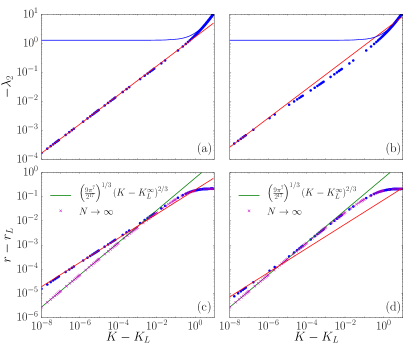
Figure 1: (Color online) $4^{th}$ order Runge-Kutta simulation results of the finite size Kuramoto model. Oscillator frequencies are distributed over the interval $[-1,1]$ according to the mid-point rule, Eq. (37), and $N=100$ [panels a) and c)] and $5000$ [panels b) and d)]. The locking threshold $K_{L}^{N}$ is determined numerically with an accuracy of $10^{-9}$. The Runge-Kutta integration step is 0.005 and the maximal number of iterations is $5\cdot 10^{7}$. Panels a) and b) show the square root behavior of $\lambda_{2}$ as a function of $K-K_{L}^{N}$. The red lines give our theoretical prediction, Eq. (33), with no fitting parameter, the prefactor of Eq. (33) being computed numerically for the best estimate of the locking threshold obtained. The blue lines give the large $K$ asymptotics $\lambda_{2}=-K$. Panels c) and d) show the square root behavior of $r-r_{L}$ as a function of $K-K_{L}^{N}$. The red lines give our theoretical prediction, Eq. (36), with no fitting parameter, the prefactor of Eq. (36) being computed numerically for the best estimate of the locking threshold obtained. The plots also present the infinite-$N$ limit results for $r-r_{L}$ as a function of the distance $K-K_{L}^{\infty}$ obtained by solving numerically the self consistent equation for the order parameter (crosses), as well as the $2/3$ scaling exponent prediction of Ref. [Pazó, 2005] (green line).

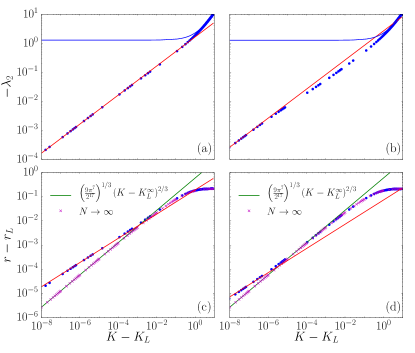
Figure 2: (Color online) Same as in Fig. 1 but for oscillator frequencies distributed according to the end-point rule, Eq. (38).

To check our main results, Eqs. (33) and (36), we numerically simulate Kuramoto models with box distributed natural frequencies and various $N$. We follow Refs. Pazó (2005); Ottino-Löffler and Strogatz (2016) and take natural frequencies evenly spaced in the interval $[-1,1]$ according either to the mid-point

$$\omega_{i}=-1+\frac{2i-1}{N}\quad i=1,\ldots,N\,,$$ (37)

or the end-point rule

$$\omega_{i}=-1+2\frac{i-1}{N-1}\quad i=1,\ldots,N\,,$$ (38)

because they allow to obtain leading-order estimates for $K_{L}^{N}$ and $r_{L}^{N}$, Eqs. (39) and (40) below. Few results we obtained with randomly but homogeneously distributed $\omega_{i}\in[-1,1]$ corroborate the results to be presented. Figs. 1 and 2 show numerical results for $N=100$ and $N=5000$ oscillators. The data confirm the scaling predictions of Eqs. (33) and (36) sufficiently close to $K_{L}^{N}$. Thus, we report a discrepancy between the scaling of $r-r_{L}\sim(K-K_{L}^{\infty})^{2/3}$ in the thermodynamic limit and our finite size scaling which goes like $r-r_{L}\sim(K-K_{L}^{N})^{1/2}$. Some distance away from $K_{L}$, one seems to recover the $N\rightarrow\infty$ behavior $\sim(K-K_{L}^{\infty})^{2/3}$, as is evident for $N=5000$.

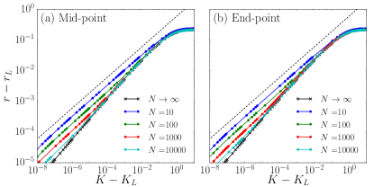
Figure 3: (Color online) Behavior of $r-r_{L}$ as a function of $K-K_{L}^{N}$ for different $N$. The coupling range above the locking threshold for which $r-r_{L}\sim(K-K_{L}^{N})^{1/2}$ decreases with the oscillator number. The dashed line indicating a $\sqrt{K-K_{L}}$ behavior is a guide to the eye.

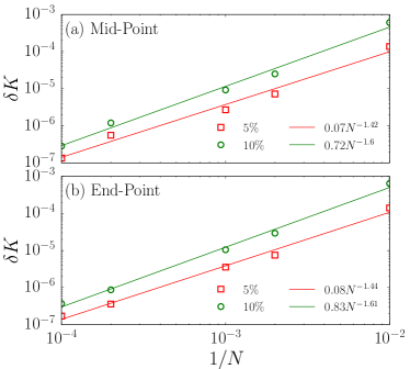
Figure 4: (Color online) Range $\delta K$ over which $r-r_{L}$ deviates from our theoretical prediction Eq. (36) by less than $5\%$ or $10\%$ as a function of the number of oscillators. Solid lines are best power-law fits.

The above reasoning predicts that the square root behavior is valid for $K$ sufficiently close to $K_{L}$, but how close? This is investigated in Figs. 3 and 4 which show that the coupling range inside which the finite size scaling holds decreases with $N$. The apparent discrepancy between Pazó’s Pazó (2005) and our results is therefore the trademark of a crossover from finite $N$ to $N\rightarrow\infty$. Fig. 4 gives the coupling range over which the numerical data obtained for $r-r_{L}$ deviates from our theoretical prediction, Eq. (36), by more than $5\%$ or $10\%$, as a function of the inverse of the oscillator number. The observed behavior suggests that the coupling range $\delta K$ inside which $r-r_{L}\sim(K-K_{L})^{1/2}$ decreases with $N$ as $\delta K\sim N^{-\alpha}$ with $\alpha\approx 1.5$ for both mid-point and end-point frequency distributions.

While we are not able to derive analytically the value of the exponent $\alpha\approx 1.5$, we can pinpoint the origin of the crossover from $r-r_{L}\sim(K-K_{L}^{N})^{1/2}$ to $r-r_{L}\sim(K-K_{L}^{\infty})^{2/3}$ as $N\rightarrow\infty$. In our treatment above we neglected terms with $l\geq 3$ in the sum over $l$ in Eq. (30). This is an increasingly bad approximation as the number of oscillators tends to infinity, because then $\lambda_{3}(K_{L}^{N})\rightarrow 0$ as $N\rightarrow\infty$. To show this, we recall the finite size asymptotics recently derived in Refs. [Pazó, 2005; Ottino-Löffler and Strogatz, 2016] for the mid-point and end-point frequency distributions, Eqs. (37) and (38). In Ref. [Ottino-Löffler and Strogatz, 2016] Ottino-Löffler and Strogatz obtained the finite-$N$ corrections (including numerical prefactors) of the locking thresholds

$$K_{L}^{N}=\left\{\begin{array}[]{l}\displaystyle\frac{4}{\pi}-\frac{64\xi}{\pi^{2}}N^{-3/2}+\mathcal{O}(N^{-2})\quad\textrm{mid-point}\,,\\[8.53581pt] \displaystyle\frac{4}{\pi}+\frac{4}{\pi}N^{-1}-\frac{64\xi}{\pi^{2}}N^{-3/2}+\mathcal{O}(N^{-2})\quad\textrm{end-point}\,,\end{array}\right.$$ (39)

where $\xi\approx 0.093366$ is the Hurwitz zeta function evaluated at $\zeta(-1/2,C_{1}/2)$, and $C_{1}\approx 0.605444$ is defined by $\zeta(1/2,C_{1}/2)=0$ with $0\leq C_{1}\leq 1$ [Quinn et al., 2007; Bailey et al., 2009]. One obtains the leading finite size corrections to the order parameter as

$$r_{L}^{N}\approx\frac{\pi}{4}+\frac{\pi}{4}(C_{1}-1)N^{-1}+\mathcal{O}(N^{-3/2})\,.$$ (40)

Despite the different scalings for the locking threshold, the asymptotic scaling of the order parameter, Eq. (40), is the same for both frequency distributions.

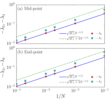
Figure 5: (Color online) Second and third largest non vanishing Lyapunov exponents at the locking threshold, for mid-point and end-point frequency distributions (panels a) and b) respectively). The solid and dashed lines give the interval defined by Eq. (42).

Mirollo and Strogatz [Mirollo and Strogatz, 2005] further showed that the spectrum of the locked state for the finite size Kuramoto model is composed of a discrete part consisting of the eigenvalues $\lambda_{1}=0$ and $-\sqrt{(Kr)^{2}-\omega^{2}}\leq\lambda_{2}\leq 0$ and of a continuous part containing the remaining $N-2$ eigenvalues $-Kr\leq\lambda_{N}\leq\ldots\leq\lambda_{3}\leq-\sqrt{(Kr)^{2}-\omega^{2}}$ where $\omega\equiv\max_{i}|\omega_{i}|$. An additional result of Ref. [Mirollo and Strogatz, 2005] is that for symmetric frequency distributions (as is the case for the mid-point and end-point rules) the Lyapunov exponents $\lambda_{3}$ and $\lambda_{4}$ can be located even more sharply as

$$-\sqrt{(Kr)^{2}-\omega_{2nd}^{2}}\leq\lambda_{4}\leq\lambda_{3}\leq-\sqrt{(Kr)^{2}-\omega^{2}}\,,$$ (41)

with $\omega_{2nd}$ the second largest frequency.

At the locking threshold, $K_{L}^{N}$ and $r_{L}^{N}$, the fully locked state is marginally stable $\lambda_{2}=0$ and expanding the bounds of Eq. (41) in powers of $N$ using Eqs. (39) and (40) gives the scaling of the gap which separates the continuous part of the spectrum from zero. Using $\omega=1-1/N$, $\omega_{2nd}=1-3/N$ and $\omega=1$, $\omega_{2nd}=1-2/N-1$ respectively for mid-point and end-point rules we obtain

$$-\frac{\sqrt{2C_{1}+4}}{\sqrt{N}}\leq\lambda_{4}\leq\lambda_{3}\leq-\frac{\sqrt{2C_{1}}}{\sqrt{N}}\,,$$ (42)

for both choices. Fig. 5 confirms numerically the scalings of $\lambda_{3}$ and $\lambda_{4}$ at $K_{L}$.

Eq. (42) then shows that at the locking threshold, $\lambda_{3,4}\sim N^{-1/2}$. This implies that the larger the number of oscillators, the closer to zero the continuous part of the spectrum will be. Thus neglecting terms with $l\geq 3$ in the sums in Eqs. (21) and (30) is an increasingly unjustified approximation as $N$ increases. The exponent $1/2$ in the behaviors of $\lambda_{2}$ and $r-r_{L}$ relies on this truncation, which is justified only in an interval $|K-K_{L}|<\delta K$ which is shrinking with $N$. To recover the $2/3$ exponent obtained by Pazó in the continuous limit would require a resummation of all terms in Eqs. (21) and (30) as $N$ tends to infinity, which we have not been able to do.

VI Conclusion

We investigated the scaling properties of the Kuramoto model with uniformly distributed natural frequencies close to the synchronization threshold at finite but growing number $N$ of oscillators. We found a non trivial behavior in that both the largest non zero Lyapunov exponent $\lambda_{2}$, and the order parameter $r$ of the fully locked state scale like $\lambda_{2}\sim(K-K_{L}^{N})^{1/2}$ and $r-r_{L}^{N}\sim(K-K_{L}^{N})^{1/2}$, above the locking threshold $K_{L}^{N}$. Our results differ from the prediction $r-r_{L}^{\infty}\sim(K-K_{L}^{\infty})^{2/3}$ of Pazó Pazó (2005) for infinitely many oscillators. We showed that this apparent disagreement is the trademark of a crossover form finite $N$ to $N\rightarrow\infty$. The range of validity $\delta K$ of our result $\lambda_{2},r-r_{L}\sim(K-K_{L}^{N})^{1/2}$ shrinks with $N$. We found numerically $\delta K\sim N^{-\alpha}$, with $\alpha\approx 1.5$. Although the numerics presented in this work are for evenly spaced frequencies, our results remain valid for other choices of $\omega_{i}$’s compatible with a uniform distribution. Our scaling predictions for $\lambda_{2}$ and $r-r_{L}$ do not depend on this choice and we checked numerically on few examples that they remain valid for frequencies drawn randomly from a uniform distribution.

The fully locked states of the Kuramoto model have been thoroughly investigated in the limit of infinitely many oscillators. For the special case of uniform frequency distributions, long-established analytical results are known for: i) the value $K_{L}^{\infty}$ of the locking threshold, ii) the value $r_{L}^{\infty}$ of the order parameter at phase locking and iii) the scaling behavior of the order parameter $r$ above $K_{L}$. For finite $N$, however, much less is known. Finite size corrections to the locking threshold and to the order parameter for frequencies uniformly distributed over the interval $[-1,1]$ have been calculated only recently Ottino-Löffler and Strogatz (2016). The motivation behind the present work is to investigate further the finite $N$ behavior of the Kuramoto close to the locking threshold. Our manuscript complements Ref. Ottino-Löffler and Strogatz (2016) by investigating the scalings of the largest Lyapunov exponent and of the order parameter above $K_{L}$. The observed crossover from finite to infinite $N$ and shrinking range of validity of our results significantly clarifies the mechanism behind the convergence to the limit $N\rightarrow\infty$ of the Kuramoto model.

References

• Kuramoto (1975) Y. Kuramoto, in International Symposium on Mathematical Problems in Theoretical Physics (Springer, Berlin, 1975), vol. 39, p. 420.
• Kuramoto (1984) Y. Kuramoto, Chemical Oscillations, Waves, and Turbulence (Springer, Berlin, 1984).
• Strogatz (2000) S. H. Strogatz, Physica D 143, 1 (2000).
• Acebrón et al. (2005) J. A. Acebrón, L. L. Bonilla, C. J. Pérez Vicente, F. Ritort, and R. Spigler, Rev. Mod. Phys. 77, 137 (2005).
• Arenas et al. (2008) A. Arenas, A. Díaz-Guilera, J. Kurths, Y. Moreno, and C. Zhou, Phys. Rep. 469, 93 (2008).
• Winfree (1967) A. T. Winfree, J. Theor. Biol. 16, 15 (1967).
• Ermentrout (1991) G. B. Ermentrout, J. Math. Biol. 29, 571 (1991).
• Wiesenfeld et al. (1996) K. Wiesenfeld, P. Colet, and S. H. Strogatz, Phys. Rev. Lett. 76, 404 (1996).
• Dörfler et al. (2013) F. Dörfler, M. Chertkov, and F. Bullo, Proc. Natl. Acad. Sci. USA 110, 2005 (2013).
• Motter et al. (2013) A. E. Motter, S. A. Myers, M. Anghel, and T. Nishikawa, Nat. Phys. 9, 191 (2013).
• Coletta et al. (2016) T. Coletta, R. Delabays, I. Adagideli, and P. Jacquod, New J. Phys. 18, 103042 (2016).
• Mirollo and Strogatz (2005) R. E. Mirollo and S. H. Strogatz, Physica D 205, 249 (2005).
• Aeyels and Rogge (2004) D. Aeyels and J. A. Rogge, Prog. Theor. Phys. 112, 921 (2004).
• Jadbabaie et al. (IEEE, Piscataway, NJ, 2004) A. Jadbabaie, N. Motee, and M. Barahona, in Proceedings of the American Control Conference (IEEE, Piscataway, NJ, 2004), p. 4296.
• Pazó (2005) D. Pazó, Phys. Rev. E 72, 046211 (2005).
• Ottino-Löffler and Strogatz (2016) B. Ottino-Löffler and S. H. Strogatz, Phys. Rev. E 93, 062220 (2016).
• van Hemmen and Wreszinski (1993) J. L. van Hemmen and W. F. Wreszinski, J. Stat. Phys. 72, 145 (1993).
• Dörfler and Bullo (2011) F. Dörfler and F. Bullo, J. Appl. Dyn. Syst. 10, 1070 (2011).
• Verwoerd and Mason (2011) M. Verwoerd and O. Mason, J. Appl. Dyn. Syst. 10, 906 (2011).
• Cohen-Tannoudji et al. (1977) C. Cohen-Tannoudji, B. Diu, and F. Laloë, Quantum Mechanics (Wiley, New York, 1977).
• Horn and Johnson (1986) R. A. Horn and C. R. Johnson, Matrix Analysis (Cambridge University Press, New York, 1986).
• Ermentrout (1985) G. B. Ermentrout, J. Math. Biol. 22, 1 (1985).
• Quinn et al. (2007) D. D. Quinn, R. H. Rand, and S. H. Strogatz, Phys. Rev. E 75, 036218 (2007).
• Bailey et al. (2009) D. H. Bailey, J. M. Borwein, and R. E. Crandall, Exp. Math. 18, 107 (2009).